Conformer: Embedding Continuous Attention in Vision Transformer
for Weather Forecasting

Abstract

Operational weather forecasting system relies on computationally expensive physics-based models. Although Transformers-based models have shown remarkable potential in weather forecasting, Transformers are discrete models which limit their ability to learn the continuous spatio-temporal features of the dynamical weather system. We address this issue with Conformer, a spatio-temporal Continuous Vision Transformer for weather forecasting. Conformer is designed to learn the continuous weather evolution over time by implementing continuity in the multi-head attention mechanism. The attention mechanism is encoded as a differentiable function in the transformer architecture to model the complex weather dynamics. We evaluate Conformer against a state-of-the-art Numerical Weather Prediction (NWP) model and several deep learning based weather forecasting models. Conformer outperforms some of the existing data-driven models at all lead times while only being trained at lower resolution data.

1 Introduction

We address the non-continuity problem in Vision Transformer (ViT) which arise in weather forecasting systems where data is present in discrete form. Operational weather forecasts systems rely on physics based Numerical Weather Prediction (NWP) models. NWP models use high performance and massively parallel super computers to model the change in weather variables. These models use virtual 3D grid systems to represent the physical systems of the Earth. Governing differential equations are solved numerically to model the dynamic components of the Earth such as ocean and atmosphere (Nguyen et al., 2023b; Bi et al., 2023). While highly accurate, these system suffer from several limitations. They tend to be extremely slow, requiring several days to run simulations which is not feasible for real-time predictions. Also, the numerical solutions of these complex differential equations require high computational resources usually hundreds of thousands of GPU nodes which is unfeasible (Bauer et al., 2020). Moreover, the introduction of approximation errors can result in false weather predictions (Palmer et al., 2005) and the level of domain knowledge needed to run these simulations can be a huge hindrance in deploying these systems for natural disaster management.

Learning continuity in discrete space-time models is a challenge. Considering the limitations of NWP systems and the popularity of Deep Learning (DL) methods, researchers have been motivated to explore the potential benefits of data-driven methodologies in weather forecasting. These systems are trained on historical weather data to produce future forecasts without explicitly defining the atmospheric physical laws. Existing state-of-the-art DL methods use Transformers (Vaswani et al., 2017), Graph Neural Networks (GNN) (Scarselli et al., 2008) and Convolutional Neural Networks (CNN) (LeCun et al., 1998) as their backbone models. However, they are considered to be discrete space and time models and do not ensure the modelling of the continuous evolving dynamics of weather system. Neural Ordinary Differential Equation (NODE) model (Chen et al., 2018) introduced the concept of continuous depth modelling to learn smooth solutions from irregular time series data. Despite being computationally efficient and accurate, Neural ODEs are only limited to temporal data and fails to learn the continuous features of spatio-temporal dynamical systems such as weather forecasting.

In this work, we build upon the core ideas of Neural ODE (Chen et al., 2018) and ViT (Dosovitskiy et al., 2020). We propose Conformer which leverages the continuous learning paradigm to effectively learn the complex spatio-temporal changes even from weather data recorded at coarser resolution. The idea is to parameterize the attention mechanism by converting it into a differentiable function. Continuous attention scores are calculated sample-wise instead of patch wise to learn the spatio-temporal mapping of weather variables in the embedding space of the vision transformer. Furthermore, we add differentiation as a pre-processing step to prepare the discrete data for continuous model and explore the role of normalization in continuous modelling.

Understanding normalization in continuous systems. Normalization is a well established concept in the field of deep learning especially in vision transformers where pre and post layer normalization optimize gradient propagation under different settings. The influence of different normalization techniques in neural ODEs was also explored by Gusak et al. (2020), however, the role of normalized derivatives is still poorly understood in spatio-temporal forecasting tasks such as weather forecasting. We empirically investigate the influence of normalization in forecasting different weather variables. We observed that normalizing the continuous evolution of hidden layers yields different results for each predicted weather variable.

In this paper we focus on the following research question: Can we design a data-driven weather forecasting system that is computationally efficient, learns the continuous latent representation and achieves precision levels commensurate with Numerical Weather Prediction (NWP) model. In summary, our contributions are as follows:

1. We propose continuous attention to effectively learn and interpolate the spatio-temporal information for weather forecasting.

2. We introduce differentiation as a pre-processing step to ensure better feature extraction for continuous spatio-temporal models.

3. Finally, we explore the role of normalized derivatives in the prediction of different weather variables.

2 Background

Attention in Vision Transformers. The attention mechanism plays a crucial role in capturing long-term spatial dependencies. While the concept of attention in vision has been discussed in literature for decades, it gained popularity with the introduction of Vision transformers (Dosovitskiy et al., 2020). The attention mechanism capture relationships between different patches by attending to relevant information using Query, Key and Value.

$Attention(Q,K,V)=softmax(\frac{QK^{T}}{\sqrt{d_{k}}})V$

The ability of attention mechanism to contextualize information yields remarkable results in several domains.

Neural ODEs. Neural ODEs are the continuous time models which learn the evolution of a system over time using Ordinary Differential Equations (ODE) (Chen et al., 2018). The solution of the system is similar to solving an Initial Value Problem. The input layer $x_{0}$ is considered as the initial condition (input value at time $t_{0}$) and the solution of the system is obtained using integration as a backpropagation technique. $\int^{T}_{0}\frac{dx(t)}{dt}=\int^{T}_{0}f(x,t,\theta)$. Neural ODEs provide an effective way to learn the continuous evolution of hidden representations over time making them fit for modelling irregular time-series data while being computationally efficient.

3 Related Work

NWP Weather Forecasting Models. These models are based on a set of differential equations solved using given initial conditions and model changes of the system over time. Some of the advanced systems include the thermo-hydrodynamical equation based weather forecasting system (Fuhrer et al., 2018) which runs simulations on Piz Diant supercomputer using nearly 5000 GPUs to generate predictions at 1.9 km resolution. Another cutting-edge forecasting system named DYAMOND (Stevens et al., 2019) solves Navier-Stokes equation to measure turbulent motions of the atmosphere. The experiments are initialized using European Centre for Medium Range Weather Forecasts (ECMWF) 9 km observations.

Integrated Forecasting System (IFS) (ECMWF, 2023) is the operational NWP based weather forecasting system which generates forecasts at a high resolution of 1km. IFS combines data assimilation and earth system model to generate accurate forecasts using high computing super computers. Despite generating accurate forecasts at high resolutions, NWP models are require days to run simulations. Moreover, thousands of GPU nodes and exceptional computational power of supercomputers are required to perform forecasting simulations leading to the ineffective usage of these models for day to day weather forecasting tasks with limited computational power.

Deep Learning Weather Forecasting Models. The success of Deep Learning (DL) has given rise to the development of weather forecasting systems using data-driven methodologies based on low computational costs as compared to NWP models. WeatherBench (Rasp et al., 2020) provides a benchmark platform to evaluate data-driven systems for effective development of weather forecasting models. Some state-of-the-art DL based models include Keisler implemented a message passing Graph Neural Network (GNN) based forecasting model (2022). ClimaX (Nguyen et al., 2023a) was introduced as a foundation model for weather and climate forecasting. The authors used Vision Transformer (ViT) as a backbone for spatio-temporal forecasting on number of tasks i.e. global forecasting, regional forecasting and seasonal forecasting each with a lead time of several hours, days and months.

FourCastNet (FCN) (Kurth et al., 2023) used a combination of Fourier Neural Operator (FNO) and ViT and was reported to be 80,000 times faster than NWP models. Pangu-Weather (Bi et al., 2023) was introduced which was designed to encode 3D earth pressure levels to reduce the forecasting errors. GraphCast (Lam et al., 2023) used a multi-mesh GNN based model for forecasts and recently, Stormer (Nguyen et al., 2023c) based on transformer model emerged as the state-of-the-art weather forecasting model. While being highly accurate, these models are discrete space-time models and do not encode the continuous dynamics of weather system.

Variants of Vision Transformer The idea of vision transformers (Dosovitskiy et al., 2020) was first introduced in 2020 and immense research has been done on the topic since then. A variant of vision transformers was introduced which was trained on a medium sized dataset and overcame the drawback of requiring large amounts of data for training a ViT (Touvron et al., 2021). A Token to Token ViT (Yuan et al., 2021) was proposed which focused on making the architecture more efficient by shortening the token length. Cross-Covariance image Transformer (XCiT) (Ali et al., 2021) solved the problem of quadratic complexity of ViTs due to long sequence of tokens and attention mechanism. XCiT could be trained on images with high resolution due to it’s linear complexity. Furthermore, different ViT architectures were introduced combined with convolutional layers. They were designed as a hybrid of attention mechanism with convolutions (Wu et al., 2021; Xu et al., 2021; Hassani et al., 2021).

Self-supervised learning paradigm was also explored using ViTs. Self-distillation with no labels DINO (Caron et al., 2021) was able to perform pixel level segmentation without directly being trained on the pixel level data. Efficient self-supervised Vision Transformer (EsViT) (Li et al., 2021) proposed patch-level self supervision mechanism which outperformed fully supervised ViTs. Though ViTs effectively learn the contextual information, modelling continuous dynamics from discrete time step data is still a challenge. We address this challenge by designing a ViT based architecture to adapt to dynamical systems like weather forecasting and learn the data representations and changes occurring within this data over time.

4 Methodology

4.1 Problem Formulation

Consider a model $f$ receives weather data as input of the form $(X^{N\times W\times H},t)$ where $N$ is the number of weather variables such as temperature, wind speed, pressure, etc., $H\times W$ refers to the spatial resolution of the variable and $t$ is the lead time over which the system evolves. The model takes weather variables at time $t_{\circ}$, learns the spatio-temporal system evolution from $t$ to $t+1$ and predicts the weather at next time step $X_{t+1}$.

$\hat{X}(t)=f(X,t)$ where $X=X(t_{\circ})$

Since the weather changes continuously over time, it is also important to capture the continuous change within the provided fixed time data. The idea is to to learn the continuous latent representation of the weather data using differential equation solvers. In such a way, the model not only predicts the value of weather variable at time ’T’ but, the definite integral also learns the changes in weather variable such as temperature from initial time to time ’T’. The system can be represented as:

$\frac{dX(t)}{dt}=f(X,t,\theta)$

$\int^{T}_{0}\frac{dX(t)}{dt}=\int^{T}_{0}f(X,t,\theta)$

$X(t)=[f(X,t,\theta)]^{T}_{0}$

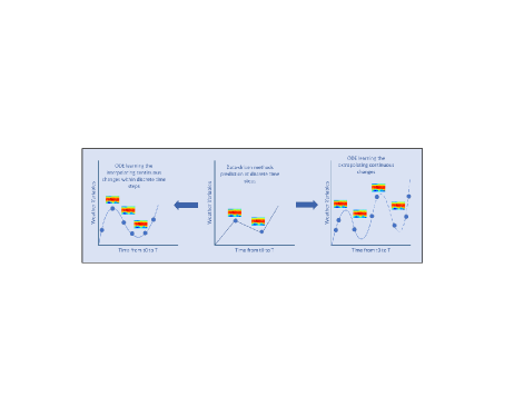
Figure 1: Differential equation learning paradigm: Learning the interpolating changes to predicts weather at next time step.

4.2 Differentiation as a pre-processing step

Weather information is highly variational and complex at both temporal and spatial levels. Temporal derivatives of each weather variable are calculated to preserve weather dynamics and ensure better feature extraction from discretized data. We perform sample wise differentiation at pixel level to capture the continuous changes in weather events over time.

$\frac{dV(x,y,t)}{dt}=\frac{V(x,y,t)-V(x,y,t-1)}{\Delta t}$

where $V(x,y,t)$ is pixel value of weather variable at time t and $V(x,y,t-1)$ is the pixel value of same variable at t-1. Figure 2 shows the graphical representation of the pre-processing step.

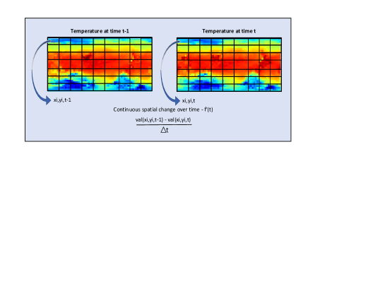
Figure 2: Pixel wise temporal differentiation to capture the spatial changes in weather variables occurring over time.

4.3 Normalized Derivatives

Normalization of derivatives is one of the crucial steps to encode stability in the behavior of deep learning model. While the effects and results of different normalization techniques in neural ODEs has been explored before (Gusak et al., 2020), it only looks at normalization as layers in the neural network architecture. We extend the idea by investigating the role of normalization when directly applied to derivatives. We applied two normalization most common techniques namely min-max and z-score normalization followed by the pre-differentiation layer to showcase their benefits in continuous systems. Experimental analysis of normalization and its effects on forecasting accuracy of geopotential and temperature is given in figure 3.

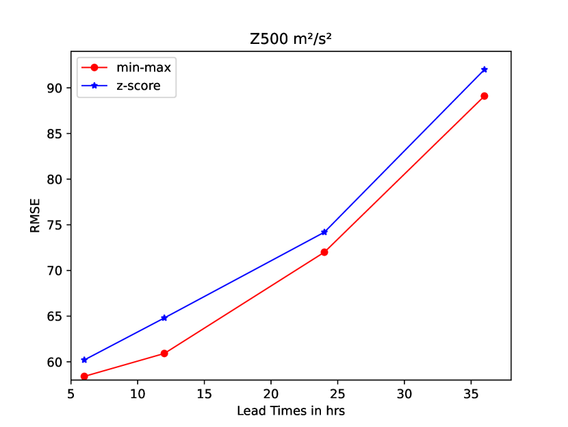
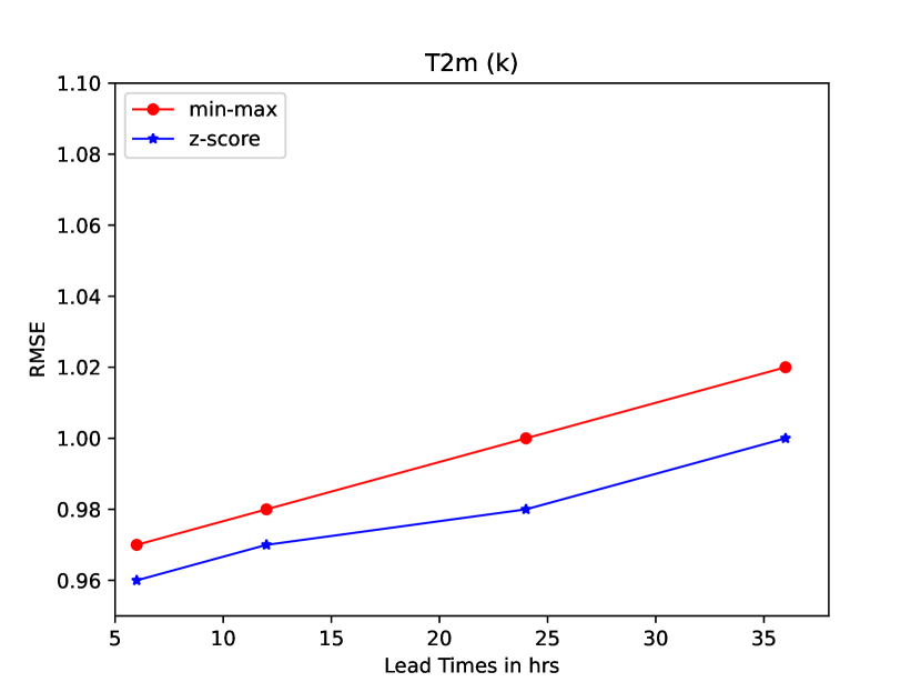
Figure 3: RMSE (lower is better) comparison for z500 and T2m to highlight the effect of different normalization techniques. Geopotential (z500) performs better with min-max while temperature (T2m) performs better with z-score normalization.

4.4 Continuous Attention

Attention is one of the key components in the vision transformer architecture. It is based on the idea of determining the most crucial parts of image in the final prediction stage. Despite being successful in variety of tasks, ViT is still restrictive in its ability to learn informative embedding for a highly dynamical system like weather forecasting. We design continuous attention mechanism to model the the continuous evolving state of weather variables. The detailed workflow of continuous attention is shown in figure 4. First, we replace the patch-wise attention with the sample-wise attention to calculate the contextual embedding space for each weather variable evolving with time. This step will ensure that rather than attending to patches within the same image, the model attends to the same variable across different images within the batch. Variable transformation is learned by assigning each variable with its own Query, Key, and Value across each input sample, similar to how it’s done within a single image. The attention mechanism calculates the attention scores between the variables of different samples (across the same variable positions). Similar to traditional attention mechanisms, the attention weights obtained across batches can be used to aggregate or weigh the information associated with those variables.

This modification allows the model to capture relationships or dependencies between the same weather variables across different instances. It proved to be beneficial in weather forecasting scenario where the model is able to map the continuous evolving features of each weather variable. To ensure continuous learning, we introduce derivatives in the sample wise attention mechanism. Differential equations represent the dynamics of the physical system with respect to time and cater to the missing values of data. We combined the attention mechanism with the differential equation learning paradigm to model the change of the atmosphere for both the spatial and temporal features. Moreover, this approach removes the limitation of modelling complex physics equations in NWP models. Furthermore, instead of having predictions at particular time stamp only, Conformer learns the transitional changes from one time step to another which is important for capturing unprecedented changes in weather.

To compute continuous attention, we calculate derivatives of similarity across same variables of each data sample. Assume we have two input samples of size $(N\times W\times H)$ denoted as $X_{0}$ at time $t_{0}$ and $X_{1}$ at time $t_{1}$ where $N$ is the number of weather variables such as temperature, wind speed, pressure, etc., $H\times W$ refers to the spatial resolution of the variable. Each variable has its own Q, K, and V tensors across both samples. Given $Q_{t_{0},i}$ and $K_{t_{1},j}$ are the Query and Key representations for the $i_{th}$ variable at time $t_{0}$ and $j_{th}$ variable at time $t_{1}$. Continuous attention is computed as follows:

$\frac{d}{dt}(Q_{t_{0},i}).(K_{t_{1},j})=Q_{t_{0},i}\frac{d(K_{t_{1},j})}{dt}+K_{t_{1},j}\frac{d(Q_{t_{0},i})}{dt}$

$Q_{t_{0},i}\frac{d(K_{t_{1},j})}{dt}+K_{t_{1},j}\frac{d(Q_{t_{0},i})}{dt}=Y$

Cont-Att($Q_{t_{0},i}$ , $K_{t_{1},j}$) = Softmax$(\frac{Y}{\sqrt{d_{k}}})$

$Output_{t_{0},t_{1}}$ = $\sum\limits^{N}_{k=1}$Cont-Att($Q_{t_{0},i}$ , $K_{t_{1},j}$) . $V_{t_{1},j}$

The resulting output represents the attention weighted sum of values for similar variables across input samples at time $t_{0}$ and $t_{1}$. This information captures relationships or dependencies between corresponding variables across the input samples at different time steps. This process calculates attention between similar variables across input samples at all time steps, allowing the model to capture relationships or interactions between variables across the entire sequence of input samples.

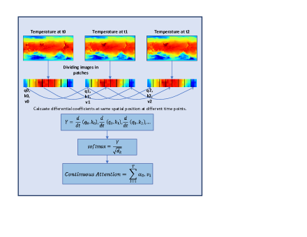
Figure 4: Continuous Attention methodology to capture the change in weather information with respect to time.

4.5 Neural ODE Layer

To further enhance the learning of continuous features of weather information, we add Neural ODE layers to the model. Since adaptive-size solvers have higher accuracy than fixed-size step solvers, we choose Dormad Prince (Dopri5) to learn the smallest possible change in weather with respect to time. Dopri5 provides us with the advantage of adaptive time stepping which perform six evaluations of function to provide a more accurate solution even at coarse resolution of $5.625^{\circ}$. The complete workflow of Conformer and placement of Neural ODE layers is shown in Figure 5. The DOPRI equation is given as follows.

$$y_{k+1}=y_{k}+\frac{35}{384}k_{1}+\frac{500}{1113}k_{3}+\frac{125}{194}k_{4}-\\ \frac{2187}{6784}k_{5}+\frac{11}{84}k_{6}$$ (1)

where $y_{k+1}$ and $y_{k}$ are states of the system at current and next time step. $k_{1},k_{3},k_{4},k_{5}$ and $k_{6}$ are provided in appendix A.

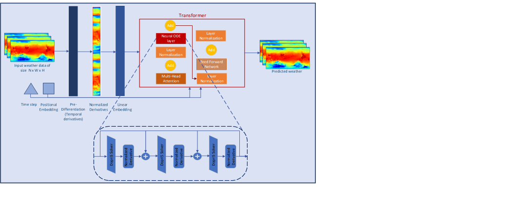
Figure 5: Workflow diagram of Conformer

5 Experiments

5.1 Dataset

We used WeatherBench (Rasp et al., 2020) to download the ERA5 (Hersbach et al., 2018, 2020) dataset provided by the European Center for Medium-Range Weather Forecasting (ECMWF) for training our model. ERA5 is a weather reanalysis dataset of hourly intervals that provides data over several parameters such as land, ocean and atmosphere. The real-time data with the highest resolution of $0.25^{\circ}\times 0.25^{\circ}$ is being collected since 1940 till date. ERA5 is considered to be the most physically accurate dataset as it is based on data assimilation methodology in which new forecasts are continuously combined with previous forecasts in such a way that resultant is consistent with laws of physics. We trained our model on $5.625^{\circ}$ resolution of ERA5 provided by WeatherBench. Table 1 provides a detail of weather variables in ERA5 dataset.

Table 1: ERA5 dataset variables and their atmospheric pressure values

Variable name	Abbreviation
(Atmospheric variables at 7 levels)
Geopotential	(Z)
U Wind Component	(U)
V Wind Component	(V)
Temperature	(T)
Specific Humidity	(Q)
Relative Humidity	(R)
(Static Variables)
Land-sea mask	(LSM)
Orography
2 meter Temperature	(T2m)
10 meter U Wind Component	(U10)
10 meter V Wind Component	(V10)

5.2 Evaluation Metrics

We used Root Mean Square Error (RMSE) and Anomaly Correlation Coefficient to evaluate our model predictions. The formula used for RMSE is:

RMSE = $\frac{1}{N}\sum\limits^{N}_{k=1}\sqrt{\frac{1}{H\times W}\sum\limits^{H}_{i=1}\sum\limits^{W}_{j=1}L(i)(\hat{X}_{k,i,j}-X_{k,i,j})^{2}}$

where $H\times W$ is the spatial resolution of the weather input and N is the number of total samples used for training or testing. L(i) is used to account for non-uniformity in grid cells.

ACC = $\frac{\sum_{k,i,j}\hat{X^{\prime}}_{k,i,j}X^{\prime}_{k,i,j}}{\sqrt{\sum_{k,i,j}L(i)\hat{X^{\prime}}^{2}_{k,i,j}\sum_{k,i,j}L(i)X^{\prime 2}_{k,i,j}}}$

Where $\hat{X^{\prime}}=\hat{X^{\prime}}-C$ and $X^{\prime}=X^{\prime}-C$ and C is the temporal mean of the entire test set $C=\frac{1}{N}\sum_{k}X$

5.3 Implementation Details

A tensor of shape $N\times H\times W$ is fed to the pre-processing layer of the model where it passes through pre-differentiation to Conformer and outputs a tensor of $N^{\prime}\times H^{\prime}\times W^{\prime}$. Hyperparameters of the model are given in the table 2 in Appendix A.

5.4 Inference and Training times

Training Times. Conformer is trained separately for each time lead with the intervals of 6 hrs. Our model is trained using 8 NVIDIA RTX A5000 GPUs of 24 GB memory. Training Conformer takes about 5 days which is orders of magnitudes faster and computationally efficient than most data-driven weather forecasting methodologies such as GraphCast (Lam et al., 2022) which took 4 weeks to train on 32 TPU devices, FourCastNet (Kurth et al., 2023) required supercomputing powers and ClimaX (Nguyen et al., 2023a) was trained on 80 NVIDIA V100 GPUs.

Inference Times. Conformer can output forecasts results at several lead times at which it is trained on. It takes less than 20 seconds to output a forecast using a single GPU.

5.5 Ablation Studies

We performed extensive empirical analysis to understand the role of different components in our model’s performance. The results of ablation study shows that while Neural ODE is a powerful architecture, it outperforms vanilla architectures when embedded in attention mechanism. All ablation studies are performed on $5.625^{\circ}$ resolution ERA5 reanalysis data. The results comparison is shown in Figure 6 and 7.

Continuous Attention only model. To understand the importance of continuous attention, we remove the neural ODE layer and provide the output of attention mechanism to the basic feed forward network. While continuous attention only model does not outperform the Conformer, it provide better prediction accuracy than the regular patch-wise attention model. The results show that continuous attention aids in the learning of highly dynamic features of weather information.

Continuous Attention vs Neural ODE layer. We perform another ablation study to compare how well Neural ODE capture continuity in weather information when simply added as a layer in the transformer architecture. Neural ODE (Chen et al., 2018) is a continuous depth neural network designed to perform like a ResNet architecture and learn continuous information in the process as well. For this study, we replace the continuous attention with regular patch-wise attention and add a Neural ODE layer in the feed forward block. The feed forward solution is approximated using Runge-Kutta (RK) numerical solver. RK solves high order differential equation by treating them as initial value problems with low computational cost.

Replacing Conformer with a basic Vision Transformer Vision Transformer has emerged as a powerful architecture which captures long-term dependencies better than any model. However, this ablation study shows the limitation of ViT in representing the dynamical systems such as weather forecasting. For this ablation study, we simply train a basic ViT architecture on ERA5 dataset. Compared with Conformer, not only ViT under performs for prediction accuracy, it is also computationally expensive. This could be explained due to the replacement of patch-wise attention with sample-wise attention in Conformer.

Vanilla Neural ODE Network. Another ablation study is done using vanilla Neural ODE model. We replace the transformer with Neural ODE architecture as proposed in the original paper (Chen et al., 2018). While Neural ODEs are computationally efficient, they only aid in interpolating the temporal irregularities and ignore the spatial continuity. This study proves that Conformer learns both spatio-temporal continuous features from the discrete data and is better at representing dynamical forecast systems.

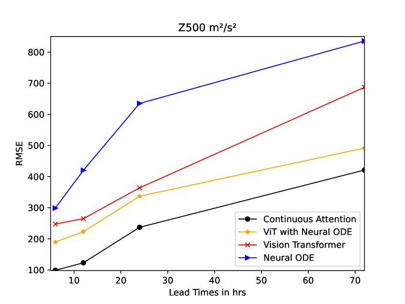
Figure 6: RMSE (lower is better) comparison for z500 to highlight the importance of each component of Conformer. Compared with vanilla Neural ODE and ViT architectures, continuous attention outperforms all of them.

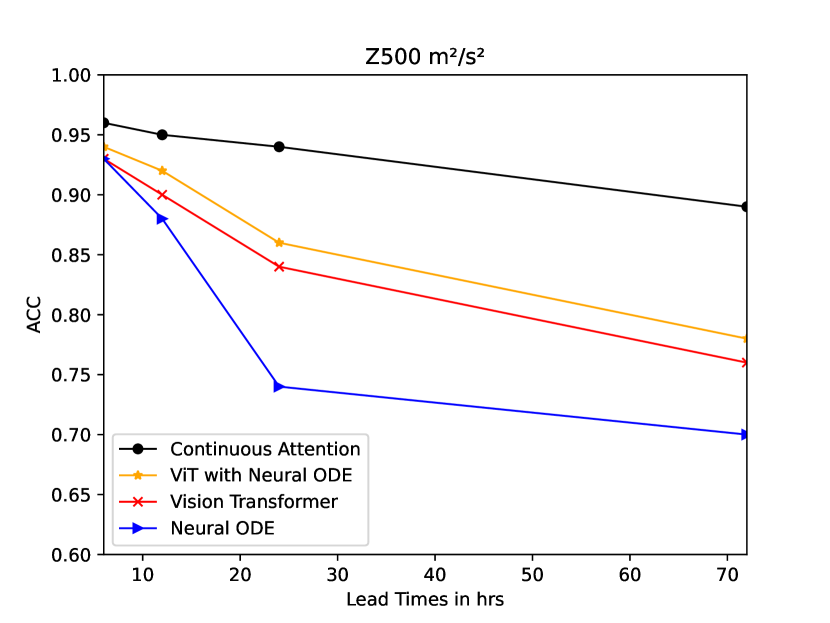
Figure 7: ACC (higher is better) comparison for z500 to highlight the importance of each component of Conformer. Compared with vanilla Neural ODE and ViT architectures, continuous attention outperforms all of them.

6 Results and Discussion

We compare Conformer’s forecast performance with ClimaX, IFS, FourCastNet at $5.625^{\circ}$ resolution. The forecast results of ClimaX were obtained using both methodologies described in the paper i.e. first with pre-training, calling it as pre-climaX and second without pre-training simply as climaX. We obtain prediction results for temperature at 2m (T2m), 10m U wind component (U10), 10m V wind component (V10), temperature at 850hpa (T850) and geopotential at 500hpa(z500). Conformer is trained for time leads with intervals of 6hrs from short-range to medium-range to long-range weather forecasting. We also compare Conformer’s performance at $5.625^{\circ}$ resolution with the results of FourCastNet, GraphCast and PanguWeather at a higher resolution of $0.25^{\circ}$.

Conformer outperforms ClimaX and FourCastNet at all times which leads us to a conclusion that replacing regular attention with continuous attention in ViT architecture derives improved feature extraction by mapping the changes occurring between successive time steps. Conformer also outperforms FourCastNet trained at $0.25^{\circ}$ resolution. While Conformer does not outperform the two most popularly used weather forecasting models Pangu and GraphCast at shorter lead times, it still performs better at longer lead times which shows the supremacy of ViT architectures at capturing long term dependencies even when trained at coarser resolution data. RMSE results are given in figure 8. ACC results are given in table 3 in Appendix B.

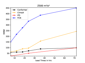
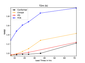
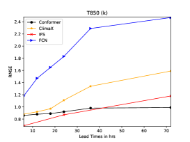
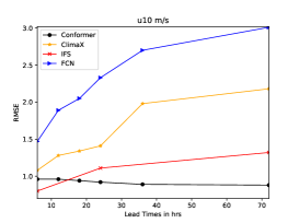
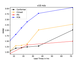
Figure 8: RMSE comparison of Conformer on ERA5 at $5.625^{\circ}$ resolution

7 Conclusion and Future Work

Abrupt changes in weather has given rise to the need of more accurate weather forecasting systems. Accurate weather prediction is a need of today’s world. Moreover, we require systems that can be used in real-time on devices with moderate computational power. Understanding the changes in weather patterns leads us to better decision making and helps in mitigating the disastrous effects of natural hazards occurring due to climate change. In this paper, we move one step closer to capturing those continuous weather changes along with predicting the weather at future time steps. We presented Conformer, a novel technique designed to capture continuous dynamics of weather data. Conformer addresses the limitations of NWP and data-driven methodologies by introducing the concept of continuous attention for modelling spatio-temporal features of weather data. The continuous attention accounts for any errors present in observational data as it not only looks at the provided specific time stamp data, but also learns the interpolation of spatial and temporal changes within the observed time stamp data.

Currently, there is immense research being done on implementing foundation models for weather forecasting. While Conformer performs really well for weather forecasting system, it is still a black-box model. Building an interpretable weather forecasting model could be a major goal for future work. Moreover, there is still limited research on extreme event forecasting. Since, Conformer performs better at capturing continuous changes in weather, extending our methodology to identify and predict extreme weather patterns presents an opportunity as future research. Finally, we aim to generalise this methodology for all other types of spatio-temporal data.

Impact Statement

This paper presents work whose goal is to advance the field of Machine Learning,with applications in climate science and weather forecasting. There are many potential societal consequences of our work, none which we feel must be specifically highlighted here.

Appendix A Implementation Details for Reproducibility

A.1 Hyperparameters

Table 2: Hyperparameters of Conformer

Hyperparameters	Meaning	Value
N	Number of variables	48
p	Patch size	4
cont-layers	Number of continuous attention layers	12
node-layer	Number of neural ode layers	3
Depth	Number of ViT Blocks	6
Dimension	Hidden dimension of prediction head	1024
Dropout	Dropout rate	0.1

A.2 Dormand Prince Equations

$k_{1}=hf(x_{i},y_{i})$

$k_{2}=hf(x_{i}+\frac{1}{5}h,y_{i}+\frac{1}{5}k_{1})$

$k_{3}=hf(x_{i}+\frac{3}{10}h,y_{i}+\frac{3}{40}k_{1}+\frac{9}{40}k_{2}$

$k_{4}=hf(x_{i}+\frac{4}{5}h,y_{i}+\frac{44}{45}k_{1}-\frac{56}{15}k_{2}+\frac{32}{9}k_{3})$

$k_{5}=hf(x_{i}+\frac{8}{9}h,y_{i}+\frac{19372}{6561}k_{1}-\frac{25360}{2187}k_{2}+\frac{64448}{6561}k_{3}-\frac{212}{729}k_{4})$

$k_{6}=hf(x_{i}+h,y_{i}+\frac{9017}{3168}k_{1}-\frac{355}{33}k_{2}+\frac{46732}{5247}k_{3}+\frac{49}{176}k_{4}-\frac{5103}{18656}k_{5})$

Appendix B Result Summary

Table 3: ACC comparison of Conformer on ERA5 at $5.625^{\circ}$ resolution

Variable	Lead Time (hr.)	Architecture
		Conformer	ClimaX	IFS (Integrated Forecast System)	FourCastNet
T2m	6	0.99	0.98	0.99	0.99
	12	0.99	0.98	N/A	0.99
	18	0.99	0.97	N/A	0.99
	24	0.98	0.96	0.98	0.99
	36	0.98	0.94	N/A	0.98
	72	0.98	0.94	0.96	0.98
T850	6	0.99	0.98	0.99	0.99
	12	0.99	0.97	N/A	0.99
	18	0.99	0.97	N/A	0.99
	24	0.99	0.97	0.99	0.98
	36	0.98	0.96	N/A	0.98
	72	0.98	0.95	0.96	0.98
z500	6	0.99	1.00	1.00	0.99
	12	0.99	1.00	N/A	0.99
	18	0.99	0.99	N/A	0.99
	24	0.98	0.98	0.99	0.99
	36	0.98	0.98	N/A	0.98
	72	0.98	0.97	0.98	0.98
u10	6	0.98	0.97	0.98	0.93
	12	0.98	0.96	N/A	0.91
	18	0.98	0.96	N/A	0.89
	24	0.96	0.94	0.97	0.89
	36	0.94	0.92	N/A	0.87
	72	0.92	0.85	0.89	0.86
v10	6	0.96	0.95	0.98	0.95
	12	0.96	0.95	N/A	0.91
	18	0.94	0.94	N/A	0.88
	24	0.92	0.85	0.97	0.85
	36	0.89	0.84	N/A	0.84
	72	0.88	0.80	0.89	0.82

References

- Ali et al. (2021) Ali, A., Touvron, H., Caron, M., Bojanowski, P., Douze, M., Joulin, A., Laptev, I., Neverova, N., Synnaeve, G., Verbeek, J., et al. Xcit: Cross-covariance image transformers. Advances in neural information processing systems, 34:20014–20027, 2021.
- Bauer et al. (2020) Bauer, P., Quintino, T., Wedi, N., Bonanni, A., Chrust, M., Deconinck, W., Diamantakis, M., Düben, P., English, S., Flemming, J., et al. The ECMWF scalability programme: Progress and plans. European Centre for Medium Range Weather Forecasts, 2020.
- Bi et al. (2023) Bi, K., Xie, L., Zhang, H., Chen, X., Gu, X., and Tian, Q. Accurate medium-range global weather forecasting with 3d neural networks. Nature, pp. 1–6, 2023.
- Caron et al. (2021) Caron, M., Touvron, H., Misra, I., Jégou, H., Mairal, J., Bojanowski, P., and Joulin, A. Emerging properties in self-supervised vision transformers. In Proceedings of the IEEE/CVF international conference on computer vision, pp. 9650–9660, 2021.
- Chen et al. (2018) Chen, R. T., Rubanova, Y., Bettencourt, J., and Duvenaud, D. K. Neural ordinary differential equations. Advances in neural information processing systems, 31, 2018.
- Dosovitskiy et al. (2020) Dosovitskiy, A., Beyer, L., Kolesnikov, A., Weissenborn, D., Zhai, X., Unterthiner, T., Dehghani, M., Minderer, M., Heigold, G., Gelly, S., et al. An image is worth 16x16 words: Transformers for image recognition at scale. arXiv preprint arXiv:2010.11929, 2020.
- ECMWF (2023) ECMWF. Ifs documentation cy48r1. ecmwf. 2023.
- Fuhrer et al. (2018) Fuhrer, O., Chadha, T., Hoefler, T., Kwasniewski, G., Lapillonne, X., Leutwyler, D., Lüthi, D., Osuna, C., Schär, C., Schulthess, T. C., et al. Near-global climate simulation at 1 km resolution: establishing a performance baseline on 4888 gpus with cosmo 5.0. Geoscientific Model Development, 11(4):1665–1681, 2018.
- Gusak et al. (2020) Gusak, J., Markeeva, L., Daulbaev, T., Katrutsa, A., Cichocki, A., and Oseledets, I. Towards understanding normalization in neural odes. arXiv preprint arXiv:2004.09222, 2020.
- Hassani et al. (2021) Hassani, A., Walton, S., Shah, N., Abuduweili, A., Li, J., and Shi, H. Escaping the big data paradigm with compact transformers. arXiv preprint arXiv:2104.05704, 2021.
- Hersbach et al. (2018) Hersbach, H., Bell, B., Berrisford, P., Biavati, G., Horányi, A., Muñoz Sabater, J., Nicolas, J., Peubey, C., Radu, R., Rozum, I., et al. Era5 hourly data on single levels from 1959 to present [dataset]. copernicus climate change service (c3s) climate data store (cds), 2018.
- Hersbach et al. (2020) Hersbach, H., Bell, B., Berrisford, P., Hirahara, S., Horányi, A., Muñoz-Sabater, J., Nicolas, J., Peubey, C., Radu, R., Schepers, D., et al. The era5 global reanalysis. Quarterly Journal of the Royal Meteorological Society, 146(730):1999–2049, 2020.
- Keisler (2022) Keisler, R. Forecasting global weather with graph neural networks. arXiv preprint arXiv:2202.07575, 2022.
- Kurth et al. (2023) Kurth, T., Subramanian, S., Harrington, P., Pathak, J., Mardani, M., Hall, D., Miele, A., Kashinath, K., and Anandkumar, A. Fourcastnet: Accelerating global high-resolution weather forecasting using adaptive fourier neural operators. In Proceedings of the Platform for Advanced Scientific Computing Conference, pp. 1–11, 2023.
- Lam et al. (2022) Lam, R., Sanchez-Gonzalez, A., Willson, M., Wirnsberger, P., Fortunato, M., Pritzel, A., Ravuri, S., Ewalds, T., Alet, F., Eaton-Rosen, Z., et al. Graphcast: Learning skillful medium-range global weather forecasting. arXiv preprint arXiv:2212.12794, 2022.
- Lam et al. (2023) Lam, R., Sanchez-Gonzalez, A., Willson, M., Wirnsberger, P., Fortunato, M., Alet, F., Ravuri, S., Ewalds, T., Eaton-Rosen, Z., Hu, W., et al. Learning skillful medium-range global weather forecasting. Science, pp. eadi2336, 2023.
- LeCun et al. (1998) LeCun, Y., Bottou, L., Bengio, Y., and Haffner, P. Gradient-based learning applied to document recognition. Proceedings of the IEEE, 86(11):2278–2324, 1998.
- Li et al. (2021) Li, C., Yang, J., Zhang, P., Gao, M., Xiao, B., Dai, X., Yuan, L., and Gao, J. Efficient self-supervised vision transformers for representation learning. arXiv preprint arXiv:2106.09785, 2021.
- Nguyen et al. (2023a) Nguyen, T., Brandstetter, J., Kapoor, A., Gupta, J. K., and Grover, A. Climax: A foundation model for weather and climate. arXiv preprint arXiv:2301.10343, 2023a.
- Nguyen et al. (2023b) Nguyen, T., Jewik, J., Bansal, H., Sharma, P., and Grover, A. Climatelearn: Benchmarking machine learning for weather and climate modeling. arXiv preprint arXiv:2307.01909, 2023b.
- Nguyen et al. (2023c) Nguyen, T., Shah, R., Bansal, H., Arcomano, T., Madireddy, S., Maulik, R., Kotamarthi, V., Foster, I., and Grover, A. Scaling transformer neural networks for skillful and reliable medium-range weather forecasting. arXiv preprint arXiv:2312.03876, 2023c.
- Palmer et al. (2005) Palmer, T., Shutts, G., Hagedorn, R., Doblas-Reyes, F., Jung, T., and Leutbecher, M. Representing model uncertainty in weather and climate prediction. Annu. Rev. Earth Planet. Sci., 33:163–193, 2005.
- Rasp et al. (2020) Rasp, S., Dueben, P. D., Scher, S., Weyn, J. A., Mouatadid, S., and Thuerey, N. Weatherbench: a benchmark data set for data-driven weather forecasting. Journal of Advances in Modeling Earth Systems, 12(11):e2020MS002203, 2020.
- Scarselli et al. (2008) Scarselli, F., Gori, M., Tsoi, A. C., Hagenbuchner, M., and Monfardini, G. The graph neural network model. IEEE transactions on neural networks, 20(1):61–80, 2008.
- Stevens et al. (2019) Stevens, B., Satoh, M., Auger, L., Biercamp, J., Bretherton, C. S., Chen, X., Düben, P., Judt, F., Khairoutdinov, M., Klocke, D., et al. Dyamond: the dynamics of the atmospheric general circulation modeled on non-hydrostatic domains. Progress in Earth and Planetary Science, 6(1):1–17, 2019.
- Touvron et al. (2021) Touvron, H., Cord, M., Douze, M., Massa, F., Sablayrolles, A., and Jégou, H. Training data-efficient image transformers & distillation through attention. In International conference on machine learning, pp. 10347–10357. PMLR, 2021.
- Vaswani et al. (2017) Vaswani, A., Shazeer, N., Parmar, N., Uszkoreit, J., Jones, L., Gomez, A. N., Kaiser, Ł., and Polosukhin, I. Attention is all you need. Advances in neural information processing systems, 30, 2017.
- Wu et al. (2021) Wu, H., Xiao, B., Codella, N., Liu, M., Dai, X., Yuan, L., and Zhang, L. Cvt: Introducing convolutions to vision transformers. In Proceedings of the IEEE/CVF international conference on computer vision, pp. 22–31, 2021.
- Xu et al. (2021) Xu, W., Xu, Y., Chang, T., and Tu, Z. Co-scale conv-attentional image transformers. In Proceedings of the IEEE/CVF International Conference on Computer Vision, pp. 9981–9990, 2021.
- Yuan et al. (2021) Yuan, L., Chen, Y., Wang, T., Yu, W., Shi, Y., Jiang, Z.-H., Tay, F. E., Feng, J., and Yan, S. Tokens-to-token vit: Training vision transformers from scratch on imagenet. In Proceedings of the IEEE/CVF international conference on computer vision, pp. 558–567, 2021.