Generalized Bayesian Additive Regression Trees for Restricted Mean Survival Time Inference

Abstract

Prediction methods for time-to-event outcomes often utilize survival models that rely on strong assumptions about noninformative censoring or on how individual-level covariates and survival functions are related. When the main interest is in predicting individual-level restricted mean survival times (RMST), reliance on such assumptions can lead to poor predictive performance if these assumptions are not satisfied. We propose a generalized Bayes framework that avoids full probability modeling of all survival outcomes by using an RMST-targeted loss function that depends on a collection of inverse probability of censoring weights (IPCW). In our generalized Bayes formulation, we utilize a flexible additive tree regression model for the RMST function, and the posterior distribution of interest is obtained through model-averaging IPCW-conditional loss function-based pseudo-Bayesian posteriors. Because informative censoring can be captured by the IPCW-dependent loss function, our approach only requires one to specify a model for the censoring distribution, thereby obviating the need for complex joint modeling to handle informative censoring. We evaluate the performance of our method through a series of simulations that compare it with several well-known survival machine learning methods, and we illustrate the application of our method using a multi-site cohort of breast cancer patients with clinical and genomic covariates.

Keywords: dependent censoring, ensemble methods, Gibbs posterior, inverse weighting, loss function, survival analysis

1 Introduction

The restricted mean survival time (RMST) is a measure that has emerged as a valuable quantity in survival analysis due to its direct clinical interpretation, which holds regardless of the survival model used in an analysis (Royston & Parmar (2013)). The RMST is defined as the expected survival duration up to a pre-specified truncation time $\tau$. Changes in RMST are often cited as an alternative to hazard ratios in the context of treatment comparisons and in survival regression modeling (Pak et al. (2017); Kloecker et al. (2020)). An advantage of using RMST is that differences in RMST are model free in the sense that, unlike proportional hazards, the interpretation of change in RMST holds regardless of whether or not a particular survival regression model holds. Moreover, constructing a prognostic model that directly targets the RMST as a function of baseline covariates can be a useful tool because the interpretation of each estimated RMST is transparent and does not require a proportional hazards assumption plus additional modeling of a baseline hazard function.

To estimate the RMST as a function of a patient’s baseline covariates, there are a number of available approaches. For instance, one could specify a full probability model for the survival outcomes, such as an accelerated failure time (AFT) model where the RMST emerges as a function of other model parameters. Another possible option is to estimate RMST by using estimates of both the baseline hazard and regression parameters from a Cox proportional hazards model. An alternative to these approaches that avoids full probability modeling of the survival outcomes is to plug in RMST-targeted “pseudo-observations” as the responses (e.g., Andersen et al. (2004) and Zhao (2020)) and treat these pseudo-observations as fully observed responses. One can then directly use more well-known regression or machine learning techniques to estimate RMST. Another attractive approach which also avoids full probability modeling is to use the inverse probability of censoring weights (IPCW; Robins et al. (1993)) as part of an objective function that only uses the observed event times. IPCW-based approaches have been used by numerous authors in the context of estimating regression models for RMST. For example, Tian et al. (2014) proposed using IPCW to estimate a class of linear regression models that target RMST. Wang & Schaubel (2018) described an approach that uses weighted estimating equations with IPCW to estimate a collection of RMSTs in the context of dependent censoring, and Zhong & Schaubel (2022) also proposed a similar strategy to estimate regression models for RMST at a collection of truncation points. Xiang & Murray (2012) combined the pseudo-outcome approach with IPCW to estimate the restricted mean of a log-survival time under dependent censoring.

An advantage of using IPCW is its ability to directly handle informative censoring where the survival and censoring times are not independent but are conditionally independent given certain patient covariate information. With IPCW, one does not need to specify a joint model for survival and censoring times as such modeling can be quite complex and involve the specification of model features that are not directly related to the RMST. Rather, one can model the censoring distribution separately from the objective function used for RMST estimation and then plug the estimated censoring probabilities into an RMST-driven objective function.

Our main goal in this work is to bridge IPCW approaches for estimating RMST with flexible Bayesian models for inference. Combining these approaches can harness the advantages of Bayesian procedures for uncertainty quantification and the robustness and simplicity of IPCW-based procedures. However, a major obstacle when seeking to incorporate IPCW as part of a Bayesian procedure for performing inference about a collection of RMST values is that IPCW does not directly fit into the classical Bayesian framework. Typically, estimation of an RMST function using IPCW is performed by solving a weighted estimating equation where the uncertainty in the weights is ignored and where the estimating equation may or may not have any connection with an appropriate log-likelihood. To address this, we propose basing inferences about an RMST function around the loss function-driven “generalized Bayes” framework described in Bissiri et al. (2016). This generalized Bayes framework has recently seen increasing popularity and has been deployed in a variety of contexts, for example, in clustering (Rigon et al. (2023)) and in estimating the distribution of a categorical outcome under dataset shift (Fiksel et al. (2022)). The main feature of generalized Bayes is that it provides a mechanism to update a prior to a posterior distribution even when one has not specified a full joint probability model for all components involved and has only specified a loss function of interest. The pseudo-Bayesian posterior distribution resulting from such a prior-updating procedure is often referred to as a “Gibbs posterior” (Martin & Syring (2022)). Using a generalized Bayes approach allows us to directly target the RMST function of interest without needing to choose a model that completely describes the distribution of the survival outcomes. This allows us to avoid having to model nuisance parameters, which makes both the model specificication and posterior computation less cumbersome. Moreover, it allows our inferences about the RMST function to be more robust to model misspecification. Indeed, as noted in Jiang & Tanner (2001), when model misspecification is present, the performance of a likelihood-based Bayesian procedure can be sub-optimal for a risk function of interest even though the posterior may be consistent for a model that is closest, in the Kullback-Leibler sense to the true model.

The procedure we propose for finding a Gibbs posterior of an RMST function is not, however, an exact application of the generalized Bayes updating procedure described in Bissiri et al. (2016). This is because the natural IPCW loss function for RMST includes weights that depend on features of the unknown censoring distribution, and hence, the loss function of interest depends on the censoring distribution. To handle this, we propose an updating procedure that can be seen as arising from two steps. First, we form a censoring distribution-conditional Gibbs posterior for the RMST function by applying the generalized Bayes updating rule to an IPCW-driven loss function for RMST. Then, we form the final Gibbs posterior for RMST by averaging the censoring-conditional Gibbs posterior with respect to a posterior distribution for the censoring distribution.

The two-step procedure described above can be applied to any prior that one chooses for the RMST function and any likelihood-prior model that one selects for the censoring distribution. However, in this paper, we focus on a specific prior for the RMST function and two models for the censoring distribution. Specifically, we concentrate on the use of Bayesian additive regression trees (BART) priors (Chipman et al. (2010)) for the unknown RMST function, and we use a nonparametric gamma process prior for noninformative censoring and a BART-based accelerated failure time model for the case of informative censoring. BART is a flexible nonparametric prior that represents the RMST function as an ensemble of decision trees and places a regularization prior on the components of each tree. The main advantages of BART are that it can directly incorporate both continuous and categorical covariates and that BART can automatically adapt to nonlinearities and covariate interactions in the RMST function without requiring the user to specify any such interactions. We focus on BART because the emphasis of many available methods for estimating RMST from individual-level baseline covariates has been on more traditional regression models, and flexible nonparametric models which draw upon ensemble learning techniques can be a useful tool for improving the prediction of RMST in many contexts. Moreover, even though BART is closely connected to more “black box” ensemble methods, BART can still provide direct uncertainty quantification for the underlying RMST function of interest. We refer to the procedure that combines our two-stage generalized Bayes procedure with a BART prior on the RMST function as RMST-BART.

This paper is organized as follows. In Section 2, we define the RMST of a survival outcome and describe the associated covariate-dependent RMST function. Then, in Section 2, we describe a loss function that targets estimation of this RMST function, and we outline how one can use a generalized Bayes framework to bring together a model for the censoring distribution and the RMST-targeted loss function in order to generate a posterior distribution for the RMST function of interest. In addition, Section 2 describes the BART prior we use for the RMST function and details the types of models that we use to handle either noninformative or informative censoring. Section 3 discusses our default choices of all model hyperparameters, describes the selection of a loss function tuning parameter, and outlines our procedure for performing posterior computation. Section 4 reports the results of two simulation studies that evaluate the RMST-BART method and related procedures under scenarios with both noninformative and informative censoring mechanisms. Section 5 exhibits the uses of our method with an analysis of a breast cancer study that contains clinical and genomic covariates, and we then conclude with a brief discussion in Section 6.

2 Loss Function-targeted generalized BART for RMST

2.1 Data Structure and Restricted Mean Survival Time

We assume that we have a study with $n$ cases or individuals with the random variable $T_{i}$ denoting the time-to-failure of an event of interest for individual $i$ and the random variable $C_{i}$ denoting a time of right-censoring for this time-to-event outcome. We observe the vector of follow-up times $\mathbf{U}=(U_{1},\ldots,U_{n})$ and vector of event indicators $\mbox{\boldmath$\delta$}=(\delta_{1},\ldots,\delta_{n})$, where $U_{i}=\min\{T_{i},C_{i}\}$ and $\delta_{i}=I(T_{i}\leq C_{i})$. For each pair $(U_{i},\delta_{i})$, we observe a corresponding vector $\mathbf{x}_{i}$ of baseline covariates.

Of primary interest are the restricted mean survival times (RMST) for transformed survival times $b(T_{i})$, where $b$ is a monotone increasing function. For an individual with covariate vector $\mathbf{x}_{i}$, the RMST parameter $\mu_{\tau}(\mathbf{x}_{i})$ with restriction point $\tau$ for the transformed survival times $b(T_{i})$ is defined as the expectation of the minimum of $b(T_{i})$ and $\tau$ conditional on the value of the covariate vector $\mathbf{x}_{i}$. Specifically, the $\tau$-RMST of $b(T_{i})$ is defined as

$$\mu_{\tau}(\mathbf{x}_{i})=E[\min\{b(T_{i}),\tau\}\mid\mathbf{x}_{i}]=E[b(U_{i}^{\tau})\mid\mathbf{x}_{i}],$$

where $U_{i}^{\tau}$ is the random variable $U_{i}^{\tau}=\min\{U_{i},b^{-1}(\tau)\}$. The connection between the $\tau$-RMST and the area under the survival function of $b(T_{i})$ from $0$ to $\tau$ is frequently noted (e.g., Royston & Parmar (2013)). Specifically, if $S(t|\mathbf{x}_{i})=P\{b(T_{i})>t|\mathbf{x}_{i}\}$, then $\mu_{\tau}(\mathbf{x}_{i})$ can be expressed as

$$\mu_{\tau}(\mathbf{x}_{i})=\int_{0}^{\tau}S(t|\mathbf{x}_{i})dt.$$

2.2 A Loss Function for RMST

Suppose we are considering a function $f(\mathbf{x}_{i})$ which takes a covariate vector $\mathbf{x}_{i}$ as input and whose purpose is to target the $\tau$-RMST of the transformed survival time $b(T_{i})$. If we assumed the censoring-survival distribution conditional on $\mathbf{x}_{i}$, i.e., $G(t|\mathbf{x}_{i})=P(C_{i}>t|\mathbf{x}_{i})$, was known, a natural inverse probability of censoring weighted (IPCW) loss function to evaluate the performance of $f(\cdot)$ is the following

$$\mathcal{L}_{\eta}(f|\Lambda;\mathbf{U}^{\tau},\mbox{\boldmath$\delta$})=\eta\sum_{i=1}^{n}\delta_{i}\exp\{\Lambda(U_{i}^{\tau}|\mathbf{x}_{i})\}\big{[}b(U_{i}^{\tau})-f(\mathbf{x}_{i})\big{]}^{2},$$ (1)

where $\mathbf{U}^{\tau}=\big{(}\min\{U_{1},\tau\},\ldots,\min\{U_{n},\tau\}\big{)}$ denotes the $n\times 1$ vector of $\tau$-truncated follow-up times and where $\eta>0$ is a positive scalar. In Equation (1), $\Lambda(t|\mathbf{x}_{i})$ is the censoring cumulative hazard function conditional on the value of $\mathbf{x}_{i}$. Under the assumption that the censoring survival function $G(t|\mathbf{x}_{i})$ is continuous in $t$ for each $\mathbf{x}_{i}$, $G(t|\mathbf{x}_{i})=\exp\{-\Lambda(U_{i}^{\tau}|\mathbf{x}_{i})\}$, and hence, using weights $\exp\{\Lambda(U_{i}^{\tau}|\mathbf{x}_{i})\}$ is equivalent to using inverse censoring weights $1/G(t|\mathbf{x}_{i})$.

The justification for considering a loss function of the form (1) is that, under the assumption of independence of $T_{i}$ and $C_{i}$ given $\mathbf{x}_{i}$, the expected value of the following expected discrepancy

$$E\Big{\{}\delta_{i}\exp\{\Lambda(U_{i}^{\tau}|\mathbf{x}_{i})\}\big{[}b(U_{i}^{\tau})-\theta_{i}\big{]}^{2}\Big{|}\mathbf{x}_{i}\Big{\}}$$

is minimized by setting $\theta_{i}=\mu_{\tau}(\mathbf{x}_{i})$, for $i=1,\ldots,n$. IPCW-based objective functions similar to that in equation (1) have been used in other approaches to modeling the RMST in a regression context, including, for example, Tian et al. (2014) and Wang & Schaubel (2018). More generally, many fundamental estimates in survival analysis can be viewed through the lens of IPCW-based estimation; for example, as noted in Satten & Datta (2001), the Kaplan-Meier estimator can be characterized as a weighted empirical distribution function using the observed event times with the inverse censoring probabilities as weights.

Our main aim is to use the IPCW-based loss function (1) to drive inferences about $f()$, and we do not want our inference procedure to require any additional probability modeling of the survival times $T_{i}$. A key challenge for achieving this within a Bayesian framework is that (1) is not a log-likelihood that corresponds to a probability model that we would want to specify for the survival times, and while (1) is a reasonable objective function to target if one is only interested in generating an estimate of $f(\cdot)$, classical Bayesian inference does not provide a direct procedure for using (1) to update a prior distribution one may have for $f(\cdot)$.

One approach for updating a prior distribution when one has a loss function of interest but does not have a likelihood is the procedure described in Bissiri et al. (2016). Given our loss function of interest (1) and a prior over the unknown function $f(\cdot)$ (which we denote with $\pi_{B}$), applying the Bissiri et al. (2016) procedure for updating $\pi_{B}(\cdot)$ yields the following “Gibbs posterior” for $f$

$$p(f|\Lambda,\mathbf{U}^{\tau},\mbox{\boldmath$\delta$})=\frac{\exp\big{\{}-\mathcal{L}_{\eta}(f|\Lambda;\mathbf{U}^{\tau},\mbox{\boldmath$\delta$})\big{\}}\pi_{B}(f)}{\int\exp\big{\{}-\mathcal{L}_{\eta}(f|\Lambda;\mathbf{U}^{\tau},\mbox{\boldmath$\delta$})\big{\}}d\pi_{B}(f)}.$$ (2)

While (2) is a justifiable update of the prior $\pi_{B}(\cdot)$ when the cumulative hazard $\Lambda$ of the censoring times is known, we are chiefly interested in a “Gibbs” or “Generalized” posterior for $f(\cdot)$ which is conditional only on the observed data and does not condition on any unknown quantities. To that end, we propose to perform inference on $f(\cdot)$ by targeting the following marginal Gibbs posterior of $f$

$$p(f|\mathbf{U}^{\tau},\mbox{\boldmath$\delta$})=\int\Bigg{[}\frac{\exp\big{\{}-\mathcal{L}_{\eta}(f|\Lambda;\mathbf{U}^{\tau},\mbox{\boldmath$\delta$})\big{\}}\pi_{B}(f)}{\int\exp\big{\{}-\mathcal{L}_{\eta}(f|\Lambda;\mathbf{U}^{\tau},\mbox{\boldmath$\delta$})\big{\}}d\pi_{B}(f)}\Bigg{]}d\tilde{\pi}_{\mathbf{U}^{\tau},\boldsymbol{\delta}}(\Lambda).$$ (3)

In (3), $\tilde{\pi}_{\mathbf{U}^{\tau},\boldsymbol{\delta}}(\cdot)$ denotes a posterior distribution over $\Lambda$ based on the data $(\mathbf{U}^{\tau},\mbox{\boldmath$\delta$})$. In other words, the marginal posterior $p(f|\mathbf{U}^{\tau},\mbox{\boldmath$\delta$})$ can be thought of as arising from averaging over the $\Lambda$-conditional Gibbs posteriors $p(f|\Lambda,\mathbf{U}^{\tau},\mbox{\boldmath$\delta$})$. In practice, to sample from (3), one can simply take draws $\Lambda^{(s)}$ from $\tilde{\pi}_{\mathbf{U}^{\tau},\boldsymbol{\delta}}(\cdot)$, and for each $\Lambda^{(s)}(\cdot)$ draw $f^{(s)}$ from the Gibbs posterior in (2) using $\Lambda^{(s)}$ as the cumulative hazard function.

It is important to note that the modeling of the censoring distribution can be performed separately from the modeling of the function $f(\cdot)$. In that sense, our approach resembles conventional IPCW-based methods or propensity score methods in causal inference where the propensity score model is estimated separately from the outcome model. However, a key difference between our approach and conventional IPCW methods is that our weights are allowed to vary across MCMC iterations, and we do not just plug in a single set of weights into a loss function for $f(\cdot)$. Having variability in the weights allows for propagation of the uncertainty associated with the censoring-based weights, and separating the modeling of censoring times from the RMST loss function allows us to avoid the “model feedback” issues that could arise when trying to perform joint modeling of the RMST function and censoring probabilities (Zigler et al. (2013)). Using $\tilde{\pi}_{\mathbf{U}^{\tau},\boldsymbol{\delta}}(\cdot)$ to generate multiple samples of the IPC weights instead of using a fixed set of IPC weights can have a notable impact on the coverage performance of the credible intervals for $f(\cdot)$. Appendix B shows the results of a simulation study comparing the coverage of our approach which draws multiple samples of the IPCW with an approach which just plugs in a single set of IPCW.

2.3 Prior for $f$: Bayesian Additive Regression Trees

Bayesian additive regression trees (BART) is a flexible method originally developed to provide inferences about an unknown mean function $f(\cdot)$ that relates a vector of outcomes $\mathbf{y}\in\mathbb{R}^{n}$ with an associated design matrix of covariates $\mathbf{X}\in\mathbb{R}^{n\times p}$. BART generates a flexible, nonparametric prior for the mean function $f(\cdot)$ by assuming that $f(\cdot)$ is represented by a sum of a large collection of decision trees. Specifically, $f(\cdot)$ is assumed to have the form

$$f(\mathbf{x})=\sum_{h=1}^{H}g_{h}(\mathbf{x};\mathcal{T}_{h},\mbox{\boldmath$\mu$}_{h}),$$ (4)

where $H$ is the total number of pre-specified trees and $g_{h}(\mathbf{x};\mathcal{T}_{h},\mbox{\boldmath$\mu$}_{h})$ is the fitted value returned by the $h^{th}$ binary decision tree given an input covariate vector $\mathbf{x}$. The term $\mathcal{T}_{h}$ is a parameter representing the tree structure of the $h^{th}$ decision tree, and it contains all the necessary parameters to completely define the structure of the $h^{th}$ decision tree, including the splitting variables and splitting values used at each interior node. The term $\mbox{\boldmath$\mu$}_{h}$ is a vector that contains the fitted values for each terminal node of $\mathcal{T}_{h}$. Note that the number of elements in $\mbox{\boldmath$\mu$}_{h}$ must match the number of terminal nodes in $\mathcal{T}_{h}$. The $h^{th}$ decision tree is fully characterized by the tree structure parameter $\mathcal{T}_{h}$ and the terminal node parameters $\mbox{\boldmath$\mu$}_{h}$.

Building on (4), a prior distribution over $f(\cdot)$ is induced by placing a prior distribution over the collection of individual trees: $\{(\mathcal{T}_{1},\mbox{\boldmath$\mu$}_{1}),...,(\mathcal{T}_{H},\mbox{\boldmath$\mu$}_{H})\}$. The standard BART prior for $f(\cdot)$ assumes that $(\mathcal{T}_{1},\mbox{\boldmath$\mu$}_{1}),...,(\mathcal{T}_{H},\mbox{\boldmath$\mu$}_{H})$ are mutually independent so that the prior distribution for the collection of trees can be expressed as

$$p\big{\{}(\mathcal{T}_{1},\mbox{\boldmath$\mu$}_{1}),...,(\mathcal{T}_{H},\mbox{\boldmath$\mu$}_{H})\big{\}} = \Bigg{[}\prod_{h=1}^{H}p(\mbox{\boldmath$\mu$}_{h}|\mathcal{T}_{h})p(\mathcal{T}_{h})\Bigg{]}=\Bigg{[}\prod_{h=1}^{H}\Bigg{[}\prod_{j=1}^{n_{h}}p(\mu_{hj}|\mathcal{T}_{h})\Bigg{]}p(\mathcal{T}_{h})\Bigg{]},$$ (5)

where the vector $\mbox{\boldmath$\mu$}_{h}=(\mu_{h1},...,\mu_{hn_{h}})$ represents the $n_{h}$ terminal node parameters associated with tree $\mathcal{T}_{h}$. From equation (5), one only needs to choose the priors for $\mu_{hj}|\mathcal{T}_{h}$ and $\mathcal{T}_{h}$ in order to fully specify the BART prior for $f(\cdot)$.

Prior for $\mbox{\boldmath$\mu$}_{h}|\mathcal{T}_{h}$. For the choice of prior density $p(\mu_{hj}|\mathcal{T}_{h})$, we use a Gaussian distribution for $\mu_{hj}$, i.e., $\mu_{hj}|\mathcal{T}_{h}\sim\textrm{Normal}(\mu_{\mu},\sigma_{\mu}^{2})$, as is assumed in most other implementations of BART. While this choice of prior for $\mu_{hj}$ does indeed place prior mass on implausible values of $\mu_{hj}$ because the $\tau$-RMST function $\mu_{\tau}(\mathbf{x})$ is restricted to lie in between $b(0)$ and $\tau$, the prior probability assigned to implausible values of $\mu_{hj}$ is typically very small for choices of the prior standard deviation parameter $\sigma_{u}$ that we have found to be suitable in practice. While a prior distribution for $\mu_{hj}$ whose support is entirely contained within $(b(0),\tau)$ may seem to be more sensible in this context, using a Gaussian prior has a number of computational advantages as the conditional distribution of $\mathcal{T}_{h}$ has a closed-form expression that does not depend on $\mbox{\boldmath$\mu$}_{h}$. Default choices for the hyperparameters $(\mu_{\mu},\sigma_{\mu})$ of $p(\mu_{hj}|\mathcal{T}_{h})$ are discussed in Section 3.1.

Prior of $\mathcal{T}_{h}$. To fully specify the BART prior for $\mathcal{T}_{h}$, one needs to specify probability models for the node generation process, the splitting variable selected at each internal node, and the splitting variable selected at each internal node. For these components, we use the standard BART prior for $\mathcal{T}_{h}$ outlined in Chipman et al. (2010) with a quantile-based rule for the prior distributions of the splitting values. Namely, for the node generation process, one views the realization of the binary tree nodes as being generated from repeatedly splitting or terminating nodes until all nodes have been deemed terminal. At a given node depth $d$, a node is split upon with probability $\alpha_{*}(1+d)^{-\beta_{*}}$ and is terminated with probability $1-\alpha_{*}(1+d)^{-\beta_{*}}$. For a tree with a given collection of terminal and interior nodes, the splitting variables used at the interior nodes are selected from a discrete uniform distribution over the set of available splitting variables. Similarly, given the splitting variables chosen, the splitting value for a particular splitting variable is selected from a discrete uniform distribution over a grid of values placed at a pre-specified number of quantiles of the variable used.

One may also note that the standard BART regression model incorporates a residual variance parameter $\sigma^{2}$ and a corresponding prior, whereas our approach does not have such an explicit residual variance term. However, the tuning parameter $\eta$ in loss function (1) does play a similar role to a residual variance parameter in the sense that $\eta$ determines the relative weight given to the loss function versus the log-prior of $f(\cdot)$. Rules for selecting the tuning parameter $\eta$ are discussed in Section 3.1.

2.4 Modeling the Censoring Distribution

Modeling the censoring distribution under noninformative censoring. If one assumes censoring is noninformative, then the cumulative hazard function for censoring does not depend on any covariate information, i.e., $\Lambda(t)=\Lambda(t|\mathbf{x}_{i})$. The approach we use for modeling $\Lambda(t)$ under the assumption of noninformative censoring follows the methodology described in Sinha & Dey (1997). With this approach, one groups the data into a series of bins and places a gamma process prior (Kalbfleisch (1978); Burridge (1981)) on the increments of $\Lambda(t)$ across each bin interval. More specifically, if one constructs $J$ intervals of the form $(0,s_{1}],(s_{1},s_{2}],\ldots,(s_{j-1},s_{J}]$ using a sequence of pre-specified values $0<s_{1}<s_{2}<\ldots<s_{J}$ and considers the increment $\lambda_{j}$ of $\Lambda(t)$ across the $j^{th}$ interval $\lambda_{j}=\Lambda(s_{j})-\Lambda(s_{j-1})$, then a gamma process prior on $\Lambda(t)$ with mean process $\alpha_{0}(t)$ and rate parameter $\kappa_{0}$ implies that

$$\lambda_{j}\sim\textrm{Gamma}\big{\{}\kappa_{0}(\alpha_{0,j}-\alpha_{0,j-1}),\kappa_{0}\big{\}},$$

where $\lambda_{1},\ldots,\lambda_{J}$ are independent and $\alpha_{0,j}-\alpha_{0,j-1}=\alpha_{0}(s_{j})-\alpha_{0}(s_{j-1})$. Note that, in our parameterization of the gamma process, this implies that the prior mean and variance of $\lambda_{j}$ are $\alpha_{0,j}-\alpha_{0,j-1}$ and $1/\kappa_{0}$ respectively.

If we let $E_{j}=\sum_{i=1}^{n}(1-\delta_{i})I(s_{j-1}<U_{i}^{\tau}\leq s_{j})$ be the number of censoring events within interval $(s_{j-1},s_{j}]$ and $R_{j}=\sum_{i=1}^{n}I(U_{i}^{\tau}>s_{j-1})$ be the number at risk at $s_{j-1}$, then, as shown in Sinha & Dey (1997), the joint posterior of the increment parameters $\lambda_{j}$ given the grouped censoring data $\mathbf{E}=(E_{1},\ldots,E_{J})$ and $\mathbf{R}=(R_{1},\ldots,R_{J})$ is

$$p(\lambda_{1},\ldots,\lambda_{J}|\mathbf{E},\mathbf{R})\propto\prod_{j=1}^{J}\lambda_{j}^{\kappa_{0}(\alpha_{0,j}-\alpha_{0,j-1})-1}\exp\{-\lambda_{j}(R_{j}-E_{j}+\kappa_{0})\}\{1-\exp(-\lambda_{j})\}^{E_{j}}.$$ (6)

In order to draw a sample from the posterior of $\Lambda$ evaluated at $U_{i}^{\tau}$ (which we denote with $\Lambda^{(t)}(U_{i}^{\tau})$), we can draw $\lambda_{1},\ldots,\lambda_{J}$ from the density in equation (6), and set $\Lambda^{(t)}(U_{i}^{\tau})=\frac{\lambda_{k_{(i)}}(U_{i}^{\tau}-s_{j-1})}{s_{j}-s_{j-1}}+\sum_{k=1}^{k(i)-1}\lambda_{k}$, where $k(i)=\{j\in\{1,\ldots,J\}:s_{j-1}<U_{i}^{\tau}\leq s_{j}\}$.

Modeling the censoring distribution under informative censoring using BART. When the cumulative hazard for censoring is allowed to depend on the covariate vector $\mathbf{x}_{i}$, any Bayesian model which induces a posterior distribution over the function $\Lambda(t|\mathbf{x})$ for $0\leq t\leq b^{-1}(\tau)$ can be incorporated into our framework for targeting the marginal Gibbs posterior in (3).

In our implementation, we have modeled $\Lambda(t|\mathbf{x})$ using the nonparametric AFT model with a BART prior for the regression function described in Henderson et al. (2020). This modeling approach assumes the log-censoring times are given by

$$\log C_{i}=m^{C}(\mathbf{x}_{i})+\xi_{i},$$

where a centered Dirichlet process mixture model prior is placed on the distribution of the mean-zero residual term $\xi_{i}$ and a BART prior is placed on the function $m^{C}(\cdot)$. The above AFT model implies that the cumulative hazard functions take the form

$$\Lambda(t|\mathbf{x}_{i})=-\log\Big{\{}S_{\xi}\Big{(}\log t-m^{C}(\mathbf{x}_{i})\Big{)}\Big{\}},$$ (7)

where $S_{\xi}(t)=P(\xi_{i}>t)$ denotes the survival function of the residual term. Hence to draw one sample of $\Lambda$ from its posterior, one can use a single posterior draw of $S_{\xi}(\cdot)$ and $m^{C}(\cdot)$ and then directly apply (7).

3 Prior Specification and Posterior Computation

3.1 Choice of Hyperparameters

In the posterior computation, we use “centered” values of $b(U_{i}^{\tau})$, and our default hyperparameter settings are tailored to the centered versions of the outcomes. Because the $U_{i}^{\tau}$ are outcomes subject to right censoring, we do not perform a naive centering that simply subtracts the sample mean of $b(U_{i}^{\tau})$. Rather, we center the $b(U_{i}^{\tau})$ by subtracting an estimate of the RMST of $b(U_{i}^{\tau})$, unconditional on $\mathbf{x}_{i}$. Specifically, we let $Y_{i}^{\tau}$ denote the centered version of $b(U_{i}^{\tau})$, which is defined as

$$Y_{i}^{\tau}=b(U_{i}^{\tau})-\hat{\mu}_{b},$$

where $\hat{\mu}_{b}$ is the RMST estimate $\hat{\mu}_{b}=\frac{1}{n}\sum_{k=1}^{n}\delta_{k}b(U_{k}^{\tau})/\hat{G}^{KM}(U_{k}^{\tau})$. Here, $G^{KM}$ denotes the Kaplan-Meier estimate of the censoring distribution.

In this section, we will use $f^{c}(\mathbf{x})$ to denote the centered version of $f(\mathbf{x})$, i.e., $f^{c}(\mathbf{x})=f(\mathbf{x})-\hat{\mu}_{b}$. In practice, we place a BART prior on $f^{c}(\cdot)$ and construct our inferences about $f(\cdot)$ by simply adding $\hat{\mu}_{b}$ to draws from the posterior of $(f^{c}(\mathbf{x}_{1}),\ldots,f^{c}(\mathbf{x}_{n}))^{T}$.

Default choice of $\eta$. The term $\eta$ in the main loss function in equation (1) can be thought of as a tuning parameter that controls the weight given to loss function (1) relative to the log-prior distribution. Several procedures for selecting this type of tuning parameter have been proposed recently including Syring & Martin (2019), Holmes & Walker (2017), and Bissiri et al. (2016).

As a default choice of $\eta$, we begin with the “unit information loss” approach described in Bissiri et al. (2016). This approach balances a loss function of interest with a prior-based loss by choosing $\eta$ so that, under the assumed prior distribution, the expected value of the loss function of interest matches the expected value of a particular log-prior loss. In our context, applying the Bissiri et al. (2016) selection rule for a fixed cumulative hazard function $\Lambda$ yields the following choice of $\eta$

$$\eta=\frac{E\big{[}\log\{\pi(\tilde{\mbox{\boldmath$\theta$}}_{x})/\pi(\mbox{\boldmath$\theta$}_{x})\}\big{]}}{nE\big{[}\delta_{i}\exp\{\Lambda(U_{i}^{\tau})\}\{Y_{i}^{\tau}-f^{c}(\mathbf{x}_{i})\}^{2}\big{]}}=\frac{E\big{[}\log\{\pi(\tilde{\mbox{\boldmath$\theta$}}_{x})/\pi(\mbox{\boldmath$\theta$}_{x})\}\big{]}}{nE\big{[}\{b(T_{i}^{\tau})-\hat{\mu}_{b}-f^{c}(\mathbf{x}_{i})\}^{2}\big{]}},$$ (8)

where $T_{i}^{\tau}=\min\{T_{i},\tau\}$ and where $\mbox{\boldmath$\theta$}_{x}$ is the $n\times 1$ vector defined as $\mbox{\boldmath$\theta$}_{x}=\big{(}f^{c}(\mathbf{x}_{1}),\ldots,f^{c}(\mathbf{x}_{n})\big{)}^{T}$ and $\tilde{\mbox{\boldmath$\theta$}}_{x}$ is the maximizer of $\pi(\mbox{\boldmath$\theta$}_{x})$. In (8), the expectation in the numerator is taken with respect to the prior distribution of $\mbox{\boldmath$\theta$}_{x}$, and the expectation in the denominator is taken with respect to the prior joint distribution of $(T_{i}^{\tau},f^{c}(\mathbf{x}_{i}))$. Note that $\eta$ in (8) does not depend on $\Lambda$ due to the assumed conditional independence between $T_{i}$ and $C_{i}$ conditional on $\mathbf{x}_{i}$. Note also that because $\hat{\mu}_{b}$ just serves to center the $b(U_{i}^{\tau})$, we regard it as a fixed constant when evaluating the expectation in the denominator of (8).

To approximate the numerator of (8), we use a Gaussian process approximation to the prior distribution of $\mbox{\boldmath$\theta$}_{x}$ (i.e., $\mbox{\boldmath$\theta$}_{x}\sim\textrm{Normal}(\mathbf{0},\mbox{\boldmath$\Sigma$}_{0})$ for some covariance matrix $\mbox{\boldmath$\Sigma$}_{0}$). Under this assumption, we have that $\tilde{\mbox{\boldmath$\theta$}}_{x}=\mathbf{0}$, $\log\{\pi(\tilde{\mbox{\boldmath$\theta$}}_{x})/\pi(\mbox{\boldmath$\theta$}_{x})\}=\frac{1}{2}\mbox{\boldmath$\theta$}_{x}^{T}\mbox{\boldmath$\Sigma$}_{0}^{-1}\mbox{\boldmath$\theta$}_{x}$, and hence

$$E\Big{[}\log\{\pi(\tilde{\mbox{\boldmath$\theta$}}_{x})/\pi(\mbox{\boldmath$\theta$}_{x})\}\Big{]}=\frac{1}{2}E\Big{(}\mbox{\boldmath$\theta$}_{x}^{T}\mbox{\boldmath$\Sigma$}_{0}^{-1}\mbox{\boldmath$\theta$}_{x}\Big{)}=\frac{1}{2}\textrm{tr}\Big{(}\mbox{\boldmath$\Sigma$}_{0}^{-1}\mbox{\boldmath$\Sigma$}_{0}\Big{)}=\frac{n}{2}.$$ (9)

Combining (8) and (9), yields the unit information loss choice of $\eta=\sigma_{r}^{2}/2$, where $\sigma_{r}^{2}=E\big{[}\{b(T_{i}^{\tau})-\hat{\mu}_{b}-f^{c}(\mathbf{x}_{i})\}^{2}\big{]}.$ Because the value of the expected squared residual $\sigma_{r}^{2}$ is often difficult to specify a priori, we propose to use, as a default, the estimated residual variance $\tilde{\sigma}_{r}^{2}$ from a linear AFT model as the choice of $\sigma_{r}^{2}$. More specifically, when the number of covariates $p$ is less than or equal to $n/5$, we fit an AFT model with responses $\exp\{b(U_{i}^{\tau})\}$ with an assumed Weibull distribution for the values of $\exp\{b(U_{i}^{\tau})\}$. When $p>n/5$, we choose $\sigma_{r}^{2}$ by using the estimated residual variance $\tilde{\sigma}_{r}^{2}$ from a regularized semiparametric AFT model with responses $\exp\{b(U_{i}^{\tau})\}$, and this residual variance estimate is found using the rank-based criterion and associated fitting procedure described in Suder & Molstad (2022).

Choosing $\eta$ with cross-validation. While the default choice of $\sigma_{r}^{2}$ (and hence the default choice of $\eta=\sigma_{r}^{2}/2$) described above often works well in practice, we have found that the sensitivity to the choice of $\sigma_{r}^{2}$ is substantial enough that improved predictive performance across a wide range of scenarios can be realized by using a more intensive data-dependent choice of $\sigma_{r}^{2}$. To balance the advantages of using a data-adaptive choice of $\sigma_{r}^{2}$ with concerns about computational speed, we have found that doing 5-fold cross-validation over a small number of candidate values of $\sigma_{r}^{2}$ works quite well in practice. The six candidate values considered for $\sigma_{r}^{2}$ in cross-validation are $\{0.1\tilde{\sigma}_{r}^{2},~{}0.25\tilde{\sigma}_{r}^{2},~{}0.5\tilde{\sigma}_{r}^{2},~{}0.75\tilde{\sigma}_{r}^{2},~{}\tilde{\sigma}_{r}^{2},1.5\tilde{\sigma}_{r}^{2}\}$, where $\tilde{\sigma}_{r}^{2}$ is the default choice of $\sigma_{r}^{2}$ obtained through the procedure described above. The objective function minimized by our cross-validation procedure is an average of IPCW estimates of the RMST across each of the cross-validation test sets. The weights for these IPCW estimates are found by using the Kaplan-Meier estimates of the censoring distribution on each of the test sets.

Default choice of $\sigma_{\mu}$: As in the original formulation of BART (Chipman et al. (2010)), our default choice of $\sigma_{\mu}$ is largely driven by the observed spread of the outcomes. Because the prior for $f^{c}(\mathbf{x})$ should reflect its interpretation as a prediction for the transformed outcomes $Y_{i}^{\tau}$ whose values must satisfy $Y_{i}^{\tau}\leq\tau-\hat{\mu}_{b}$, we want our default choice of $\sigma_{\mu}$ to induce a prior distribution on $f^{c}(\mathbf{x})$ such that the prior probability assigned to the event $\{Y_{min}^{\tau}\leq f^{c}(\mathbf{x})\leq b(\tau)-\hat{\mu}_{b}\}$ is approximately $95\%$, where $Y_{min}^{\tau}$ is the minimum value of $Y_{i}^{\tau}$ among the observed events, i.e., $Y_{min}^{\tau}=\min(\{Y_{i}^{\tau}:\delta_{i}=1\})$. Because the BART prior on $f^{c}(\mathbf{x})$ implies that the variance of $f^{c}(\mathbf{x})$, conditional on the entire set of trees, is $H\sigma_{\mu}^{2}$, choosing $\sigma_{\mu}=\{b(\tau)-\hat{\mu}_{b}-b(Y_{min}^{\tau})\}/2\kappa\sqrt{H}$ with $\kappa=2$ ensures that we are assigning approximately $95\%$ prior probability for $f^{c}(\mathbf{x})$ to the interval $[Y_{min},b(\tau)-\hat{\mu}_{b}]$.

It is worth noting that there is a degree of “competition” between $\sigma_{\mu}^{2}$ and $\eta$ because smaller of values $\sigma_{\mu}^{2}$ lead to more weight being given to the prior of $f(\cdot)$ while larger values of $\eta$ lead to more weight being given to the loss function. Hence, if using either cross-validation or information-based criteria for hyperparameter tuning, trying to select $\sigma_{\mu}$ and $\eta$ simultaneously is not likely to lead to any performance improvements compared to either doing hyperparameter tuning of only $\sigma_{\mu}$ or performing hyperparameter tuning of only $\eta$. In our approach, we fix $\sigma_{\mu}$ so that the prior for $f(\cdot)$ is interpretable and only perform tuning for the loss function tuning parameter $\eta$.

Default choices of $\alpha_{*},\beta_{*}$, and $H$. For the hyperparameters $\alpha_{*}$ and $\beta_{*}$ that control the prior for the node generation process of each tree, we follow the recommendations of $\alpha_{*}=0.95$ and $\beta_{*}=2$ suggested in Chipman et al. (2010). These settings of $\alpha_{*}$ and $\beta_{*}$ ensure that most of the prior probability is assigned to smaller individual trees. For the number of trees $H$, we set $H=200$ as a default though, in our simulation studies, we do compare this with a single-tree model where $H=1$. Setting $H=200$ generally works quite well as a default and is much less computationally demanding than selecting among multiple values of $H$ using cross-validation.

Hyperparameters of the Censoring Distribution. For the noninformative censoring model of Section 2.4, one needs to specify the hyperparameters $\kappa_{0}$ and $\alpha_{0,j}-\alpha_{0,j-1}$, for $j=1,\ldots,J$. As a default, we set both $\kappa_{0}=1$ and $\alpha_{0,j}-\alpha_{0,j-1}=1$ for all $j$, because these defaults lead to a posterior distribution for $\Lambda(\cdot)$ whose mean typically does not substantially differ from the Nelson-Aalen estimator of the cumulative hazard. If substantial prior information about the censoring distribution is available, one may want to modify the values of $\alpha_{0,j}$ and $\kappa$ accordingly. As noted in Ibrahim et al. (2001), when the grid points $s_{j}$ are chosen so that the associated increment parameters $\lambda_{j}$ are not too large, setting $\kappa_{0}=1$ and $\alpha_{0,j}-\alpha_{0,j-1}=1$ ensures that the posterior of $\lambda_{j}$ in (6) has an approximate Gamma distribution with mean $(E_{j}+1)/(R_{j}-E_{j}+1)$ which is closely related to the increments of the Nelson-Aalen estimator of the cumulative hazard. An additional advantage of setting $\kappa_{0}=1$ and $\alpha_{0,j}-\alpha_{0,j-1}=1$ is that the posterior distribution of $\lambda_{j}$ is that of the logarithm of a Beta-distributed random variable with shape parameters $R_{j}-E_{j}+1$ and $E_{j}$ which makes drawing from this posterior distribution straightforward.

3.2 Posterior Computation

Our posterior computation strategy largely follows the Bayesian backfitting approach described in Chipman et al. (2010) with the addition of an update of the cumulative hazard $\Lambda(\cdot)$ in every MCMC iteration (Algorithm 1). With the Bayesian backfitting approach, one sequentially updates the pair $(\mathcal{T}_{h},\mbox{\boldmath$\mu$}_{h})$, for $h=1,\ldots,H$, by, in each MCMC iteration, utilizing the distribution of $(\mathcal{T}_{h},\mbox{\boldmath$\mu$}_{h})$ conditional on the observed data, the cumulative hazard $\Lambda(\cdot)$, and all of the other tree structures and terminal node parameters except for $(\mathcal{T}_{h},\mbox{\boldmath$\mu$}_{h})$. To elaborate further on this computational strategy, let us first re-express the $\Lambda$-conditional loss function (1) for the vector of centered outcomes $\mathbf{Y}^{\tau}=(Y_{1}^{\tau},\ldots,Y_{n}^{\tau})$ in terms of the collection of trees $\mathcal{T}=(\mathcal{T}_{1},\mathcal{T}_{2},\ldots,\mathcal{T}_{H})$ and collection of terminal node parameters $\mbox{\boldmath$\mu$}=(\mbox{\boldmath$\mu$}_{1},\ldots,\mbox{\boldmath$\mu$}_{H})$ for the centered regression function $f^{c}(\mathbf{x})$. Specifically,

$$\mathcal{L}_{\eta}(\mathcal{T},\mbox{\boldmath$\mu$}|\Lambda,\mathbf{Y}^{\tau},\mbox{\boldmath$\delta$})=\eta\sum_{i=1}^{n}\delta_{i}\exp\{-\Lambda(U_{i}^{\tau}|\mathbf{x}_{i})\}[Y_{i}^{\tau}-f^{c}(\mathbf{x}_{i})]^{2},$$

and recall that, for a fixed value of $\Lambda(\cdot)$, the posterior of interest is given by

$$p(\mathcal{T},\mbox{\boldmath$\mu$}|\Lambda,\mathbf{Y}^{\tau},\mbox{\boldmath$\delta$})\propto\exp\Big{\{}-\mathcal{L}_{\eta}(\mathcal{T},\mbox{\boldmath$\mu$}|\Lambda,\mathbf{Y}^{\tau},\mbox{\boldmath$\delta$})\Big{\}}\prod_{h=1}^{H}\pi(\mbox{\boldmath$\mu$}_{h}|\mathcal{T}_{h})\pi(\mathcal{T}_{h}).$$ (10)

Working from (10), the distribution of $(\mathcal{T}_{h},\mbox{\boldmath$\mu$}_{h})$ given $\Lambda$, the observed data, all other tree structures $\mathcal{T}_{-h}$, and all other terminal node parameters $\mbox{\boldmath$\mu$}_{-h}$ is given by

$$p(\mathcal{T}_{h},\mbox{\boldmath$\mu$}_{h}|\Lambda,\mathcal{T}_{-h},\mbox{\boldmath$\mu$}_{-h},\mathbf{Y}^{\tau},\mbox{\boldmath$\delta$})\propto\\ \exp\Big{\{}-\eta\sum_{i=1}^{n}\delta_{i}\exp\{\Lambda(U_{i}^{\tau}|\mathbf{x}_{i})\}[g_{h}(\mathbf{x}_{i})-R_{ih}]^{2}\Big{\}}\pi(\mathcal{T}_{h})\pi(\mbox{\boldmath$\mu$}_{h}|\mathcal{T}_{h}),$$ (11)

where $g_{-h}(\mathbf{x}_{i})=\sum_{k\neq h}g_{k}(\mathbf{x}_{i};\mathcal{T}_{h},\mbox{\boldmath$\mu$}_{h})$ and $R_{ih}=Y_{i}^{\tau}-g_{-h}(\mathbf{x}_{i})$ implying that $R_{ih}$ is the $i^{th}$ residual obtained from using all trees except the $h^{th}$ tree to construct the regression function. Integrating out the terminal node parameters of (11) yields the following distribution of $\mathcal{T}_{h}$ conditional on $\Lambda$, $\mathcal{T}_{-h}$, and $\mbox{\boldmath$\mu$}_{-h}$

$$p(\mathcal{T}_{h}|\Lambda,\mathcal{T}_{-h},\mbox{\boldmath$\mu$}_{-h},\mathbf{Y}^{\tau},\mbox{\boldmath$\delta$})\propto\\ \pi(\mathcal{T}_{h})\int\exp\Big{\{}-\eta\sum_{i=1}^{n}\delta_{i}\exp\{\Lambda(U_{i}^{\tau}|\mathbf{x}_{i})\}[g_{h}(\mathbf{x}_{i})-R_{ih}]^{2}\Big{\}}\pi(\mbox{\boldmath$\mu$}_{h}|\mathcal{T}_{h})d\mbox{\boldmath$\mu$}_{h}.$$ (12)

Note that $g_{h}(\mathbf{x}_{i})=\sum_{j=1}^{n_{h}}I_{jh}(\mathbf{x}_{i})\mu_{hj}$, where $I_{jh}(\mathbf{x}_{i})=1$ if $\mathbf{x}_{i}$ is assigned to the $j^{th}$ terminal node of $\mathcal{T}_{h}$ and $I_{jh}(\mathbf{x}_{i})=0$ otherwise. Hence, because the distribution $\mbox{\boldmath$\mu$}_{h}|\mathcal{T}_{h}$ is assumed to be multivariate Gaussian, the expression in (12) has a direct, closed form.

To update the $h^{th}$ tree structure in the $t^{th}$ MCMC iteration, a proposal tree $\mathcal{T}^{\prime}$ is drawn using the “grow”, “prune”, and “change” move scheme described in Chipman et al. (1998), and the proposal $\mathcal{T}^{\prime}$ is accepted or rejected using the Metropolis-Hastings ratio, which can be directly computed using (12). The update of $\mathcal{T}_{h}$ is immediately followed by an update of the terminal node parameters of the $h^{th}$ tree $\mbox{\boldmath$\mu$}_{h}$. To update $\mbox{\boldmath$\mu$}_{h}$ in the $t^{th}$ MCMC iteration, one uses the fact that, conditional on $\Lambda$, $\mathcal{T}_{h}$, $\mathcal{T}_{-h}$, and $\mbox{\boldmath$\mu$}_{-h}$, the distribution of $\mbox{\boldmath$\mu$}_{h}$ is multivariate Gaussian where the conditional mean of $\mbox{\boldmath$\mu$}_{h}$ is a weighted mean of the residuals $R_{ih}$ that is shrunken towards zero. Specifically,

$$\mbox{\boldmath$\mu$}_{h}|\Lambda,\mathcal{T}_{h},\mathcal{T}_{-h},\mbox{\boldmath$\mu$}_{-h},\mathbf{Y}^{\tau},\mbox{\boldmath$\delta$} \sim \textrm{Normal}\Big{(}\mathbf{d}_{h},\mathbf{D}_{h}\Big{)},$$ (13)

where $\mathbf{d}_{h}$ is an $n_{h}\times 1$ vector and $\mathbf{D}_{h}$ is an $n_{h}\times n_{h}$ diagonal matrix. The $j^{th}$ diagonal element $D_{jj,h}$ of $\mathbf{D}_{h}$ and the $j^{th}$ component $d_{j,h}$ of $\mathbf{d}_{h}$ are given by

$$D_{jj,h} = \frac{1}{\eta}\Big{(}(2\eta\sigma_{\mu}^{2})^{-1}+\sum_{i=1}^{n}\delta_{i}\exp\{\Lambda(U_{i}^{\tau}|\mathbf{x}_{i})\}I_{jh}(\mathbf{x}_{i})\Big{)}^{-1}$$

$$d_{j,h} = \eta D_{jj,h}\sum_{i=1}^{n}\delta_{i}\exp\{\Lambda(U_{i}^{\tau}|\mathbf{x}_{i})\}I_{jh}(\mathbf{x}_{i})R_{ih}.$$

More details about the derivation of the conditional distribution of $\mbox{\boldmath$\mu$}_{h}$ can be found in Appendix A.

Let $\mathcal{T}_{h}^{(t)}$ and $\mbox{\boldmath$\mu$}_{h}^{(t)}$ denote the values of $\mathcal{T}_{h}$ and $\mbox{\boldmath$\mu$}_{h}$ in the $t^{th}$ MCMC iteration respectively. After updating $(\mathcal{T}_{h}^{(t)},\mbox{\boldmath$\mu$}_{h}^{(t)})$ to $(\mathcal{T}_{h}^{(t+1)},\mbox{\boldmath$\mu$}_{h}^{(t+1)})$ for $h=1,\ldots,H$, one draws a new cumulative hazard $\Lambda^{(t+1)}(\cdot)$ using either the noninformative or informative censoring models described in Section 2.4. Note that the draw of $\Lambda^{(t+1)}(\cdot)$ can be performed as described in Section 2.4 because the posterior distribution of $\Lambda$ used in the target posterior (3) does not depend on the centered function $f^{c}(\cdot)$ in any way. The new cumulative hazard function $\Lambda^{(t+1)}(\cdot)$ will then be used in updates of $(\mathcal{T}_{h}^{(t+1)},\mbox{\boldmath$\mu$}_{h}^{(t+1)})$ in the subsequent MCMC iteration.

The steps needed to perform a single update of the cumulative hazard $\Lambda(\cdot)$, the collection of tree structures $\mathcal{T}_{1},\ldots,\mathcal{T}_{H}$, and terminal node parameters $\mbox{\boldmath$\mu$}_{1},\ldots,\mbox{\boldmath$\mu$}_{H}$ are summarized in Algorithm 1.

Algorithm 1 RMST-BART: One MCMC iteration to update $\Lambda$, $\mathcal{T}$, and $\mu$

Input: $\mathbf{Y}^{\tau}$, $\mathbf{X}$, $\Lambda^{(t)}(\cdot)$, $(\mathcal{T}_{h}^{(t)},\mbox{\boldmath$\mu$}_{h}^{(t)})_{h=1}^{H}$

for $h=1,...,H$ do

     1. Set: $R_{ih}=Y_{i}^{\tau}-\sum_{k=1}^{h-1}g_{k}(\mathbf{X}_{i};\mathcal{T}_{h}^{(t+1)},\mbox{\boldmath$\mu$}_{h}^{(t+1)})-\sum_{k=1}^{h+1}g_{k}(\mathbf{X}_{i};\mathcal{T}_{h}^{(t)},\mbox{\boldmath$\mu$}_{h}^{(t)})$, for $i=1,...,N$.

     2. Generate a proposal $\mathcal{T}^{\prime}$ using either a grow, change, or prune move from $\mathcal{T}_{h}$.

     3. Using (10), compute the Metropolis-Hastings ratio $\alpha_{MH}$ for $\mathcal{T}^{\prime}$ versus $\mathcal{T}_{h}^{(t)}$.

     4. Generate $u\sim$ Unif$(0,1)$.

     5. If $u\leq\alpha_{MH}$, set $\mathcal{T}_{h}^{(t+1)}=\mathcal{T}^{\prime}$; otherwise, set $\mathcal{T}_{h}^{(t+1)}=\mathcal{T}_{h}^{(t)}$.

     6. Draw $\mbox{\boldmath$\mu$}_{h}^{(t+1)}$ from the distribution in Equation (13). end for

7. Update $\Lambda^{(t+1)}(\cdot)$ by sampling from the noninformative or informative censoring model described in Section 2.4.

4 Simulations

In this section, we study the performance of the RMST-BART procedure with two simulation studies. In the first simulation study, we generate survival outcomes from a distribution whose mean is determined by the Friedman function. In our second simulation study, we draw survival outcomes from a distribution whose mean is the absolute value of a linear model where the predictors are generated from a multivariate normal distribution with a first-order autoregressive (AR(1)) Mills (1990) correlation structure. We mainly evaluate the performance of RMST-BART and competing methods on their ability to estimate the RMST function $\mu_{\tau}(\mathbf{x}_{i}^{\prime})$ on a “test set” of $\mathbf{x}_{i}^{\prime}$ values. Specifically, we assess estimation performance by recording the average root-mean squared error for $\mu_{\tau}(\mathbf{x}_{i}^{\prime})$ across simulation replications. The average RMSE performance of an estimator $\hat{\mu}_{\tau}$ was measured with the following quantity

$$\frac{1}{S}\sum_{s=1}^{S}\sqrt{\frac{1}{n_{test}}\sum_{i=1}^{n_{test}}\{\hat{\mu}_{\tau}(\mathbf{x}_{i}^{{}^{\prime},s})-\mu_{\tau}(\mathbf{x}_{i}^{{}^{\prime},s})\}^{2}},$$

where $S$ is the total number of simulation replications for a particular simulation scenario, $n_{test}$ is the number of covariate vectors in the test set, and $\mathbf{x}_{i}^{{}^{\prime},s}$ is the draw of the $i^{th}$ test set vector in the $s^{th}$ simulation replication. In addition to evaluating RMSE, we evaluated, for a subset of the simulation scenarios, the coverage proportions of the credible intervals for $\mu_{\tau}(\mathbf{x}_{i}^{\prime})$ generated by our method.

4.1 Friedman Function

For this simulation study, we draw survival outcomes $T_{i}$ from the following distribution

$$T_{i}\sim\textrm{Gamma}\Big{(}f(\mathbf{x}_{i})\{1+f(\mathbf{x}_{i})\},\{1+f(\mathbf{x}_{i})\}\Big{)},$$ (14)

where $\{1+f(\mathbf{x}_{i})\}$ represents a rate parameter implying that $E\{T_{i}\mid f(\mathbf{x}_{i})\}=f(\mathbf{x}_{i})$ and $\textrm{Var}\{T_{i}\mid f(\mathbf{x}_{i})\}=f(\mathbf{x}_{i})\{1+f(\mathbf{x}_{i})\}$. The assumed distribution of survival times in equation (14) implies that the $\tau$-RMST function for $T_{i}$ is given by

$$\mu_{\tau}(\mathbf{x}_{i}) = f(\mathbf{x}_{i})\Big{[}F_{gam}\big{(}\tau;1+f(\mathbf{x}_{i})\{1+f(\mathbf{x}_{i})\},\{1+f(\mathbf{x}_{i})\}\big{)}\Big{]}$$

$$+ \tau\Big{[}1-F_{gam}\big{(}\tau;f(\mathbf{x}_{i})\{1+f(\mathbf{x}_{i})\},\{1+f(\mathbf{x}_{i})\}\big{)}\big{)}\Big{]},$$

where $F_{gam}(x;\alpha,\beta)$ denotes the cumulative distribution function of a Gamma random variable with shape parameter $\alpha$ and rate parameter $\beta$. In equation (14), we assume that $\mathbf{x}_{i}\in\mathbb{R}^{p}$ (with $p>5$) and $f(\mathbf{x}_{i})$ is the Friedman function (Friedman (1991)) which is defined as

$$f(\mathbf{x}_{i})=10\sin(\pi x_{i1}x_{i2})+20(x_{i3}-0.5)^{2}+10x_{i4}+5x_{i5}.$$ (15)

Note that the Friedman function $f(\mathbf{x}_{i})$ only depends on the first five components of $\mathbf{x}_{i}$ and not on the last $p-5$ components. In our simulation study, we draw the components $x_{ij}$ of $\mathbf{x}_{i}=(x_{i1},\ldots,x_{ip})^{T}$ independently from a uniform distribution over $(0,1)$, i.e., $x_{ij}\sim\textrm{Uniform}(0,1)$. For the distribution of the censoring times $C_{i}$, we considered two situations: one in which censoring is noninformative, and one in which censoring is informative but $T_{i}$ and $C_{i}$ are independent given $\mathbf{x}_{i}$.

Noninformative Censoring. In this case, the censoring times $C_{i}$ are independently sampled from a gamma distribution, i.e., $C_{i}\sim\textrm{Gamma}(3.2,r)$, and we consider two different values of $r$, $r=0.1$ and $r=0.2$. When $r=0.1$, the censoring rate is relatively low with roughly $10-20\%$ of observations being censored in every simulation replication, and when $r=0.2$, the censoring rate is higher with a roughly $40-50\%$ the censoring rate in each simulation replication. For the noninformative censoring simulation scenarios, we set $\tau=25$ as the restriction point of RMST because $\tau=25$ ensures that $P(C_{i}>\tau)$ is relatively small when $r=0.2$. Specifically, when $r=0.2$ and $\tau=25$, $P(C_{i}>\tau)$ is approximately $0.15$.

Informative Censoring. For these scenarios, censoring times $C_{i}$ and $T_{i}$ are independent conditional on $\mathbf{x}_{i}$, but the distributions of both $T_{i}$ and $C_{i}$ depend on $\mathbf{x}_{i}$. In particular, the censoring times are drawn from the following distribution

$$C_{i}\sim\textrm{Gamma}\{r_{D},0.01f(\mathbf{x}_{i})\},$$ (16)

where $f(\mathbf{x}_{i})$ is the Friedman function defined in (15). The shape parameter $r_{D}$ is varied across two levels $r_{D}=1$ and $r_{D}=3$. When $r_{D}=1$, the censoring is quite “heavy” with roughly $80\%$ observations being censored, and when $r_{D}=3$, the censoring is more moderate with a roughly $40\%$ censoring rate. The reason for only considering scenarios with a $\geq 40\%$ censoring rate is to highlight performance differences between using weights $\exp\{\Lambda(U_{i}^{\tau})\}$ which do not depend on $\mathbf{x}_{i}$ and in using weights $\exp\{\Lambda(U_{i}^{\tau}|\mathbf{x}_{i})\}$ which do depend on $\mathbf{x}_{i}$, and in our experience, there is very little performance difference between these two approaches whenever censoring is very light (e.g., a $10-20\%$ censoring rate). For the informative censoring simulation scenarios, we used the same choice of restriction point (i.e., $\tau=25$) as in the noninformative censoring scenarios. The justification for choosing $\tau=25$ is that $P(C_{i}>\tau)$ is quite small when $r_{D}=1$; specifically, $P(C_{i}>\tau)\approx 0.05$.

4.2 Absolute Value Linear Model with Correlated Predictors

In this simulation study, we again simulated survival outcomes from the following distribution

$$T_{i}\sim\textrm{Gamma}\Big{(}f(\mathbf{x}_{i})\{1+f(\mathbf{x}_{i})\},\{1+f(\mathbf{x}_{i})\}\Big{)},$$

but we chose $f(\mathbf{x}_{i})$ to be a direct function of a linear combination of elements in $\mathbf{x}_{i}$. For the function $f(\mathbf{x}_{i})$, we assume that it equals the absolute value of a linear combination of the $p>5$ covariates $\mathbf{x}_{i}=(x_{i1},\ldots,x_{ip})^{T}$ with only the first $5$ of these covariates having nonzero coefficients in this linear combination. Specifically,

$$f(\mathbf{x}_{i})=\Big{|}\sum_{j=1}^{5}\beta_{j}x_{ij}\Big{|}.$$

The vector $\mathbf{x}_{i}$ is generated from a multivariate normal distribution with mean $0$ and where the components of $\mathbf{x}_{i}$ have an AR(1) correlation structure with an autoregressive parameter equal to $0.5$. That is, $\textrm{Corr}(x_{ij},x_{ik})=0.5^{|k-j|}$ and $\textrm{Var}(x_{ij})=1$.

In this simulation study, we only examined performance for the case of noninformative censoring with censoring times $C_{i}$ generated independently from $T_{i}$ using the distribution $C_{i}\sim\textrm{Gamma}(2.2,r)$. We varied $r$ across two levels: $r=1.8$ and $r=0.8$. The value $r=1.8$ was utilized to achieve a lower censoring rate (i.e., a roughly $10-20\%$ censoring rate) while $r=0.8$ was used to yield a higher censoring rate among the simulated observations (i.e., a roughly $40-50\%$ censoring rate). We set the truncation point $\tau$ to $5$ in order to yield a relatively small value of $P(C_{i}>\tau)$ when $r=0.8$. Specifically, when $\tau=5$ and $r=0.8$, $P(C_{i}>\tau)\approx 0.10$.

4.3 Simulation Results

In both simulation studies, we generated a “training set” of observations $\{(\mathbf{x}_{i},U_{i},\delta_{i});i=1,\ldots,n\}$ along with an independent “test set” of covariate vectors $\{\mathbf{x}_{i}^{\prime};i=1,\ldots,n_{test}\}$, and for each simulation study, we considered two different values for the number of observations in the training set: $n=250$ and $n=1000$. In each simulation replication, we evaluate performance with $n_{test}=1000$ separate $\mathbf{x}_{i}^{\prime}$ values in the test set. In the Friedman function simulation study with noninformative censoring, we explored two settings of the number of covariates: $p=10$ and $p=100$. In both the informative censoring scenarios of the Friedman function simulation study and in the linear model simulation study, we considered $p=10$ and $p=50$.

In both simulation studies, the average root mean squared error (RMSE) of our RMST-BART approach is compared (Tables 1, 3, and 5) with the following related methods: RMST-BART with a single tree, which we refer to as RMST-BCART due to its connection with Bayesian classification and regression trees (Chipman et al. (1998)); a Cox proportional hazards regression model (CoxPH) (Cox (1972)); an $L_{1}$-penalized Cox proportional hazards regression model (Penalized CoxPH) (Tibshirani (1997)), inverse probability of censoring weighted boosting (IPCW-boost) (Hothorn et al. (2006)); a log-normal AFT model (Wei (1992)) with only an intercept term (AFT-Null); a log-normal AFT model where the regression function for log-survival times is a linear combination of all covariates (AFT-Linear); and an AFT-based BART model (AFT-BART) (Chipman et al. (2010) and Sparapani et al. (2021)). The AFT-BART model assumes an AFT model for the survival times while placing a BART prior on the regression function and using a Gaussian distribution for the residual of the log-survival times. Note that our simulation results present two versions of the RMST-BART, RMST-BCART, and AFT-BART approaches; one which includes the “-default” suffix and one which has no suffix. The “-default” versions of RMST-BART and RMST-BCART use the default choices of $\eta$ while the versions of RMST-BART and RMST-BCART without the “-default” suffix use the value of $\eta$ found through five-fold cross-validation. The default version of AFT-BART uses all hyperparameter defaults employed in the BART package in R (Sparapani et al. (2021)), and AFT-BART performs five-fold cross-validation, as suggested in Chipman et al. (2010), with respect to three different candidate pairs of values for the hyperparameters of the residual variance parameter.

Table 1 summarizes the results from the Friedman function simulation study for the noninformative censoring case. The results presented in Table 1 indicate that, in all scenarios, our proposed method, RMST-BART, yields a lower average RMSE than the competing methods. In scenarios with light censoring, i.e., those with $r=0.1$, AFT-BART is consistently quite competitive with RMST-BART, but in scenarios where censoring is heavier, the performance gap between AFT-BART and RMST-BART is more substantial. When $n=250$, the two variations of RMST-BART, i.e., RMST-BART with the default choice of $\eta$ and RMST-BART with a cross-validation choice of $\eta$, perform quite similarly, but when $n=1000$, the larger sample size provides a clear advantage to using a cross-validation choice of $\eta$.

# of observations	$n=250$				$n=1000$
# of predictors	$p=10$		$p=100$		$p=10$		$p=100$
Method	$r=0.1$	$r=0.2$	$r=0.1$	$r=0.2$	$r=0.1$	$r=0.2$	$r=0.1$	$r=0.2$
RMST-BART-default	1.48	2.14	2.46	3.15	1.10	1.41	1.33	1.66
RMST-BART	1.54	2.10	2.37	2.82	0.62	0.83	1.08	1.64
RMST-BCART-default	3.95	4.29	5.19	5.88	3.70	4.07	4.96	4.85
RMST-BCART	3.86	4.46	5.11	6.01	3.59	4.10	4.78	4.97
CoxPH	3.30	2.93	4.05	4.43	2.83	2.62	2.90	2.84
Penalized CoxPH	3.39	3.00	3.67	3.22	2.86	2.65	2.88	2.72
IPCW-boost	2.54	2.84	2.61	2.96	2.50	2.78	2.50	2.80
AFT Null	5.38	5.34	5.35	5.35	5.34	5.35	5.34	5.33
AFT-Linear	2.81	3.05	3.80	4.84	2.76	3.03	2.87	3.12
AFT-BART-default	1.71	3.16	2.61	4.32	1.12	2.85	1.57	3.26
AFT-BART	1.70	3.17	2.61	4.31	1.12	2.85	1.57	3.26

Table 1: Friedman function simulation study. Average RMSE results for RMST-BART and related approaches. Censoring is noninformative with censoring times generated from the $\textrm{Gamma}(3.2,r)$ distribution. Two values are used for $r$: $0.1$ and $0.2$, which result in approximately $10-20\%$ and $40-50\%$ censoring rates, respectively.

Table 2 shows test-set coverage results in the Friedman function study for $95\%$ credible intervals from the following four methods: RMST-BART-default, RMST-BART (i.e., selecting $\eta$ using cross-validation), RMST-BCART, and AFT-BART. Here, average coverage of the RMST function $\mu_{\tau}(\mathbf{x}_{i})$ is computed by looking at the average coverage across points $\mathbf{x}_{i}^{\prime}$ in the test set. Specifically, we measure average coverage with

$$\frac{1}{S}\sum_{s=1}^{S}\frac{1}{n_{test}}\sum_{i=1}^{n_{test}}I\Big{\{}\hat{\mu}_{\tau}^{L}(\mathbf{x}_{i}^{{}^{\prime},s})\leq\mu_{\tau}(\mathbf{x}_{i}^{{}^{\prime},s})\leq\hat{\mu}_{\tau}^{L}(\mathbf{x}_{i}^{{}^{\prime},s})\Big{\}},$$

where $\hat{\mu}_{\tau}^{L}(\mathbf{x}_{i}^{{}^{\prime},s})$ and $\hat{\mu}_{\tau}^{U}(\mathbf{x}_{i}^{{}^{\prime},s})$ denote the lower and upper bounds of a $95\%$ credible interval for $\mu_{\tau}(\mathbf{x}_{i}^{{}^{\prime},s})$ respectively and where $\mathbf{x}_{i}^{{}^{\prime},s}$ is the draw of the $i^{th}$ test set vector in the $s^{th}$ simulation replication. For most scenarios presented in Table 2, the RMST-BART method has coverage which is fairly close to $0.95$ with coverage closer to $0.95$ than AFT-BART in all but one of the scenarios. The only case where RMST-BART coverage is notably less than $0.95$ is when censoring is heavy and the number of parameters is relatively large compared to the sample size, i.e., when $p=100$, $r=0.2$, and $n=250$, but the coverage for $p=100$ and $r=0.2$ improves notable when the sample size is increased to $n=1000$. Expectedly, the RMST-BART procedure with a single tree (i.e., RMST-BCART) typically has poor coverage as the single-tree model prior is heavily concentrated on relatively simple forms for the RMST function. While the choice of hyperparameters and the selection of $\eta$ are not explicitly constructed to target nominal frequentist coverage, our experience is that the RMST-BART $95\%$ credible intervals generally provide good coverage whenever both censoring is not extremely high and when the number of covariates is not very large relative to sample size.

# of observations	$n=250$				$n=1000$
# of predictors	$p=10$		$p=100$		$p=10$		$p=100$
Method	$r=0.1$	$r=0.2$	$r=0.1$	$r=0.2$	$r=0.1$	$r=0.2$	$r=0.1$	$r=0.2$
AFT-BART-default	0.91	0.91	0.90	0.79	0.93	0.88	0.92	0.86
RMST-BART	0.97	0.97	0.98	0.77	0.94	0.93	0.93	0.88
RMST-BCART	0.67	0.49	0.59	0.57	0.77	0.70	0.58	0.59
AFT-BART	0.91	0.83	0.90	0.79	0.93	0.88	0.92	0.86

Table 2: Average test set coverage of $95\%$ credible intervals in the Friedman function simulation study with noninformative censoring. Coverage of credible intervals from the following methods are shown: RMST-BART-default, RMST-BART, RMST-BCART, and AFT-BART.

Table 3 compares the average RMSEs for the Friedman function simulation study when censoring times are drawn from the informative censoring model (16). This table contains two settings of the censoring distribution; one with a “medium” censoring rate where $r_{D}=3$ and another with a “heavy” censoring rate where $r_{D}=1$. In the scenarios shown in Table 3, RMST-BART with covariate-dependent modeling of the IPCW (i.e., RMST-BART-DEP) usually has somewhat better RMSE performance than RMST-BART, particularly in the heavy censoring scenarios where $r_{D}=1$. The performance of RMST-BART-DEP-default which uses the default choice of $\eta$ does seem to be more sensitive to the particular simulation scenario with rather lackluster performance when $r_{D}=3$. This table also shows the impact of smaller sample sizes on the performance of RMST-BART when the covariate-dependent censoring model is used. When $n=250$ both RMST-BART and RMST-BART-DEP are outperformed by several other methods including, for example, regularized CoxPH and IPCW boosting. It is likely that when $n=250$ and, especially, when censoring is heavy the posterior draws of the IPC weights from the covariate-dependent censoring model are quite noisy, and it is only when $n=1000$ that the model learns these weights effectively enough to deliver stronger predictive performance.

Correlation	$n=250$				$n=1000$
# of predictors	$p=10$		$p=50$		$p=10$		$p=50$
Method	$r_{D}=3$	$r_{D}=1$	$r_{D}=3$	$r_{D}=1$	$r_{D}=3$	$r_{D}=1$	$r_{D}=3$	$r_{D}=1$
RMST-BART-DEP-default	4.94	3.03	5.25	5.60	3.14	1.80	3.52	2.70
RMST-BART-DEP	3.46	3.15	3.84	5.73	1.79	1.89	2.26	2.92
RMST-BART-default	4.29	3.60	4.82	6.20	2.69	1.94	3.07	3.20
RMST-BART	3.34	3.63	4.49	6.08	1.81	2.08	2.55	3.33
Coxph	3.07	3.02	3.39	5.14	2.74	2.62	2.83	2.88
Regularized Coxph	3.18	2.82	3.34	3.21	2.78	2.61	2.87	2.70
IPCW-boost	2.70	3.34	2.79	3.90	2.63	3.16	2.65	3.30
AFT Null	5.05	4.91	5.06	4.89	5.03	4.90	5.06	4.89
AFT-Linear	3.02	6.37	3.39	7.35	2.86	6.26	3.13	6.57
AFT-BART-default	2.54	6.83	3.28	6.97	2.26	7.40	2.45	7.61
AFT-BART	2.54	6.83	3.28	6.97	2.26	7.40	2.45	7.60

Table 3: Friedman function simulation study with informative censoring. Average RMSE results for RMST-BART and related approaches. Censoring times are generated using model (16). “Medium” and “heavy” censoring rates correspond to the $r_{D}=3$ and $r_{D}=1$ settings, respectively.

Table 4 shows a brief sensitivity analysis examining the impact of the choice of the key hyperparameter $\kappa$. As described in Section 3.1, the standard deviation $\sigma_{\mu}$ of the terminal node parameters is proportional to $1/\kappa$, and our default choice of $\kappa$ is $\kappa=2$. Our sensitivity analysis compares RMSE performance for four values of $\kappa$: $0.25$, $0.5$, $2$, and $4$. As shown in Table 4, using cross-validation to select $\eta$ greatly reduces the sensitivity to the choice of $\kappa$ as $\eta$ can adaptively upweight or downweight the loss function if the prior for the terminal node parameters leads to too much or too little shrinkage. However, using the default choice of $\eta$ as is done in the RMST-BART-default method makes the specific choice of $\kappa$ more meaningful. As shown in Table 4, varying $\kappa$ from $\kappa=0.5$ up to $\kappa=4$ can have a considerable impact on RMSE performance though changing $\kappa$ from $\kappa=0.5$ to $\kappa=2$ has a notable, but not as considerable of an impact. Though certainly not guaranteed to always be the best choice when using RMST-BART-default, the default choice of $\kappa=2$ has the best performance among the scenarios used in Table 4, and we have found, in our experience, that setting $\kappa=2$ serves as a good default choice across a range of other simulation experiments.

# of observations		$n=250$				$n=1000$
# of predictors		$p=10$		$p=100$		$p=10$		$p=100$
Method	$\kappa$	$r=0.1$	$r=0.2$	$r=0.1$	$r=0.2$	$r=0.1$	$r=0.2$	$r=0.1$	$r=0.2$
RMST-BART-default	0.25	2.61	3.32	3.27	3.90	1.51	2.12	1.70	2.17
RMST-BART	0.25	1.52	2.01	2.07	2.77	0.73	1.07	1.14	1.64
RMST-BART-default	0.5	1.48	2.14	2.46	3.15	1.10	1.41	1.33	1.66
RMST-BART	0.5	1.54	2.10	2.37	2.82	0.62	0.83	1.08	1.64
RMST-BART-default	2	1.41	1.78	2.07	2.90	0.70	0.90	1.05	1.43
RMST-BART	2	1.27	1.81	2.09	2.95	0.71	0.92	1.07	1.49
RMST-BART-default	4	2.62	3.05	3.32	4.00	1.50	1.99	1.70	2.10
RMST-BART	4	2.91	3.56	3.74	4.53	1.51	2.16	1.74	2.41

Table 4: Friedman function simulation study with noninformative censoring. Comparing the average RMSE results of the RMST-BART-default and RMST-BART approaches across four different values of $\kappa$.

Concluding the presentation of our simulation results, Table 5 compares the average RMSE between the RMST-BART method and alternative approaches on the absolute value linear model simulation study described in Section 4.2. In these simulation scenarios, RMST-BART performs quite well across all scenarios but is not always the top performer. In particular, the regularized Cox proportional hazards method performs the best when $n=250$ and remains a competitive method when $n=1000$. For the large sample size settings, i.e., $n=1000$, RMST-BART is the top performing method when $r=1.8$ while AFT-BART has somewhat better performance when $r=0.8$. Even though the model used for simulating survival outcomes is not exactly a Cox proportional hazards model, the strong performance of the regularized Cox proportional hazards method likely stems from the fact that the distribution of the survival times can be related directly to a linear function of the covariates, and RMST-BART often has a more impressive relative performance when the survival distribution depends on a nonlinear function of the covariates. Nevertheless, when the sample size is equal to one thousand, RMST-BART has enough data to improve upon the performance of a regularized Cox model procedure. Coverage results for this simulation study can be found in Appendix B.

# of observations	$n=250$				$n=1000$
# of predictors	$p=10$		$p=50$		$p=10$		$p=50$
Method	$r=0.8$	$r=1.8$	$r=0.8$	$r=1.8$	$r=0.8$	$r=1.8$	$r=0.8$	$r=1.8$
RMST-BART	0.65	0.70	0.73	0.72	0.59	0.59	0.65	0.68
Coxph	0.68	0.72	0.98	0.85	0.65	0.66	0.69	0.71
Regularized Coxph	0.65	0.67	0.65	0.67	0.65	0.65	0.65	0.65
IPCW-boost	0.68	0.71	0.69	0.72	0.65	0.68	0.65	0.68
AFT-Linear	0.91	1.06	1.18	1.44	0.88	0.99	0.93	1.08
AFT-BART	0.70	0.74	0.73	0.78	0.56	0.63	0.62	0.68

Table 5: Absolute value linear model simulation study. Average RMSE results for RMST-BART and related approaches. Censoring is noninformative with censoring times generated from the $\textrm{Gamma}(2.2,r)$ distribution. Two values are used for $r$: $0.8$ and $1.8$, which result in approximately $10-20\%$ and $40-50\%$ censoring rates, respectively.

5 Application

This section demonstrates the use of our methodology with a real-world dataset of breast cancer outcomes assembled by the Molecular Taxonomy of Breast Cancer International Consortium (METABRIC). This dataset comprises 1904 primary fresh-frozen breast cancer specimens that were clinically annotated and collected from tumor banks located in the UK and Canada (Pereira et al. (2016)). This dataset includes patient-level demographic and clinical variables, gene expression measures, and mutation information on $173$ genes. For our analysis, we focused on 30 covariates of interest which included $10$ variables containing gene expression measures. Among these $1904$ observations and $30$ covariates, there was a modest level of missingness in three of the covariates. To address this and prepare our data for analysis using the RMST-BART procedure, we removed all observations that had one or more missing covariate values which resulted in a final dataset of 1839 observations that we used for our analyses.

The survival outcome we targeted was overall survival measured in months. Median follow-up time among the $1839$ cases used in our analysis was quite long — 116 months, and roughly $42\%$ of these observations were censored at the time of the last follow up. For our analysis, we set the RMST-restriction point to $\tau=300$ months because this is the $96^{th}$ percentile of the estimated censoring distribution and $300$ months is a round number that has a direct interpretation as $25$ years.

Figures 1(a) and 1(b) present RMST-BART variable importance plots of the top 10 variables from both the noninformative and informative censoring models. These variable importance measures, commonly used in other applications of BART, are averages (i.e., an average across posterior draws) of the number of times a variable is used as a splitting variable among the $200$ BART trees. A comparison of these two plots reveals considerable disagreement in the top 10 variables between the informative and noninformative censoring models. Nevertheless, there are three variables that the informative and noninformative censoring models have in common: cohort membership, tumor stage, and patient age at the time of diagnosis. Regarding the cohort membership variable, this dataset divides the cases into five separate cohorts based on the time of sample collection, and the binary variable denoting membership in cohort 3 was determined to be the most important variable by both the informative and noninformative censoring models of RMST-BART. Membership in cohort 2 was also deemed to be one of the top 10 variables by both the informative and noninformative censoring models. The ten gene expression variables tended to be somewhat less important according to this measure of RMST-BART variable importance, but expression levels for CHEK2 and BRCA1 were consistently the most important among the gene expression variables.

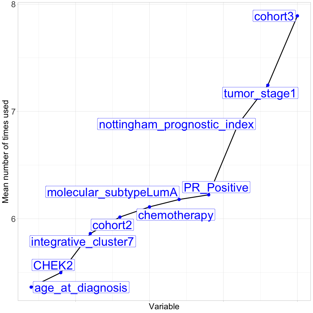
(a) Noninformative censoring

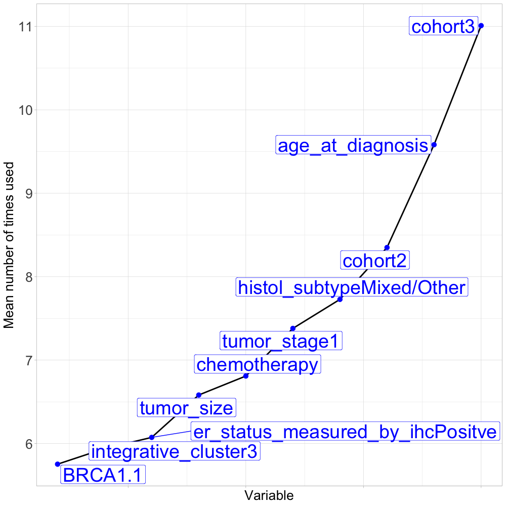
(b) Informative censoring

Figure 1: METABRIC data. Top 10 most frequently used variables by RMST-BART for both the noninformative and informative censoring models. In each case, RMST-BART used $200$ trees and $2000$ posterior draws. The y-axis represents the mean number of times a variable is used among the $200$ trees.

The RMST-BART procedure can directly generate posterior means and credible intervals for $\mu_{\tau}(\mathbf{x}_{i})$ at each covariate vector $\mathbf{x}_{i}$ represented in the study. Forest plots of posterior mean point estimates and $95\%$ uncertainty intervals for the $\mu_{\tau}(\mathbf{x}_{i})$ can provide a visual summary of the variation in the values of $\mu_{\tau}(\mathbf{x}_{i})$ and the uncertainty associated with the inference made on each individual point $\mu_{\tau}(\mathbf{x}_{i})$. Figures 2(a) and 2(b) present the RMST-BART posterior means and $95\%$ credible intervals from both the informative and noninformative censoring models. When comparing these two figures, it is apparent that the individual-level credible intervals are consistently wider in the informative censoring model and that the spread of the posterior means of the $\mu_{\tau}(\mathbf{x}_{i})$ is notably greater in the informative censoring model when compared to the noninformative censoring model. These differences are largely due to both the greater posterior uncertainty associated with the individual-level values of the cumulative hazard $\Lambda(U_{i}^{\tau}|\mathbf{x}_{i})$ and the greater range of the posterior means of $\Lambda(U_{i}^{\tau}|\mathbf{x}_{i})$ in the informative censoring model. Indeed, while both the informative and noninformative censoring models have a roughly similar median of $125$ months from their posterior mean point estimates of $\mu_{\tau}(\mathbf{x}_{i})$, the informative censoring model has a number of cases where the posterior mean is less than $50$ and a number of cases where the posterior mean of $\mu_{\tau}(\mathbf{x}_{i})$ exceeds $200$. In contrast, essentially all of the posterior mean estimates in the noninformative censoring model are between $50$ and $200$.

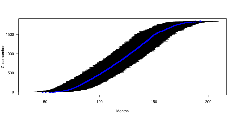
(a) Noninformative censoring

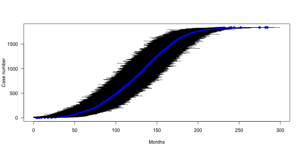
(b) Informative censoring

Figure 2: METABRIC data. Test set posterior means and credible intervals using the RMST-BART algorithm with $200$ trees and $2000$ posterior draws. Blue points represent the point estimate for each case. Posterior means and credible intervals from the noninformative censoring model are shown in the top panel while posterior means and credible intervals from the informative censoring model are shown in the bottom panel.

For ensemble methods such as RMST-BART that are more “black box” in nature, partial dependence plots (Friedman (2001)) can be a useful way to visually assess the impact of a particular covariate has on the posterior mean of the RMST function $\hat{\mu}_{\tau}(\mathbf{x})$. The partial dependence function for the $k^{th}$ covariate is defined as the expectation of a function estimator at a specific value of covariate $k$, where the expectation is taken with respect to the joint distribution of all covariates except $k$. In our context where we are interested in estimating the RMST function $\mu_{\tau}(\mathbf{x})$, the natural way of defining the estimated partial dependence function $\hat{\rho}_{k}(u)$ for covariate $k$ at point $u$ is

$$\hat{\rho}_{k}(u)=\frac{1}{n}\sum_{i=1}^{n}\hat{\mu}_{\tau}(\mathbf{x}_{i,-k},u),$$ (17)

where $\hat{\mu}_{\tau}(\mathbf{x}_{i,-k},u)$ denotes the posterior mean of $\mu_{\tau}(\mathbf{x}_{i,-k},u)$. In (17), $\mathbf{x}_{i,-k}$ is the vector that contains all of the covariates for individual $i$ except for covariate $k$, and the notation $(\mathbf{x}_{i,-k},u)$ denotes the vector where $x_{ik}=u$ and the remaining covariates are set to their observed values, i.e., $(\mathbf{x}_{i,-k},u)=(x_{i1},\ldots,x_{ik-1},u,x_{ik+1},\ldots,x_{ip})^{T}$. Plotting $\hat{\rho}_{k}(u)$ versus $u$ can provide a useful summary of how changing $x_{ik}$ influences the estimated RMST.

Figure 3 presents RMST partial dependence plots for four important continuous as identified by the RMST-BART variable importance scores. These four covariates are patient age at diagnosis, expression measurements for the BRCA1 gene, tumor size, and the “Nottingham Prognostic Index” (Galea et al. (1992)). From looking at the partial dependence plot for age at diagnosis, we can see that the highest estimated RMST values are observed in the age ranges of $55$ to $65$, followed by a clear downward trend after age 65. The steady decline after age 65 is unsurprising, but, curiously this partial dependence plot suggests moderately worse survival outcomes in younger age groups when compared to the $50-55$ age range. While this could be driven by estimation variability or other factors, this observed trend could be reflecting the fact that younger breast cancer patients have been observed to more frequently display more aggressive disease compared to older patients (Chen et al. (2016)). The importance of BRCA1 in breast cancer prognosis has been well recognized, and the partial dependence function involving BRCA1 gene expression does indeed show considerable variability across values of this variable though the relationship between standardized BRCA1 expression and predicted RMST does appear quite complex — predicted RMST remains constant in the ranges $-3$ to $0$, experiences a notable drop around $0$, and then exhibits a subsequent increase thereafter. The effect of tumor size on the partial dependence function is quite expected with increasing tumor volume being monotonically associated with estimated RMST. The Nottingham Prognostic Index is an index where larger values of the index imply a worse prognosis for breast cancer patients, and the monotone decreasing partial dependence plot in Figure 3 of this variable matches this interpretation. Interestingly, the partial dependence plot shows a sudden decrease in RMST as the Nottingham prognostic index moves from just below $4$ to just above $4$. This quick decrease likely reflects the fact that the Nottingham Prognostic Index includes the sum of two categorical variables that are treated as numeric variables, and a move from one category to another in one of the important categorical components of the index could certainly lead to a rapid decrease in the estimated RMST.

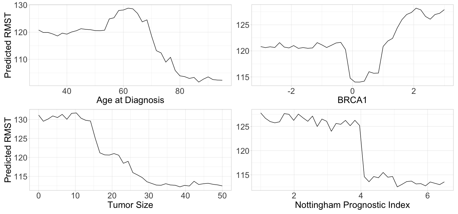
Figure 3: METABRIC data. RMST-BART partial dependence plots for the following key continuous variables: age at diagnosis, BRCA1 gene expression, tumor size, and the Nottingham Prognostic Index.

Figure 4 provides a more direct, visual comparison of the RMST-BART posterior means of $\mu_{\tau}(\mathbf{x}_{i})$ generated under the informative censoring assumption versus the posterior means generated under the noninformative censoring model. This figure shows a strong agreement between the posterior means of $\mu_{\tau}(\mathbf{x}_{i})$ produced under the two different assumptions about the censoring distribution. Indeed, the Pearson correlation between these two collections of posterior means was $0.87$. The most notable difference between these two sets of posterior means is the greater variability of the posterior means from the informative censoring model.

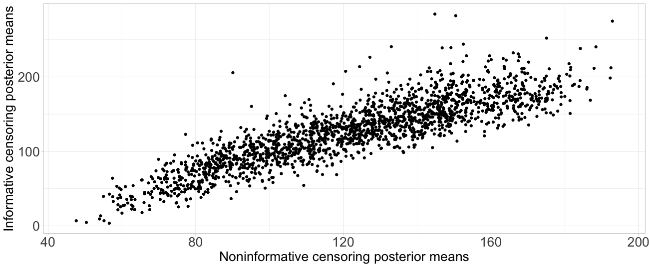
Figure 4: METABRIC data. RMST-BART posterior means under the informative censoring model versus RMST-BART posterior means under the noninformative censoring model.

6 Discussion

In this paper, we have introduced a framework for performing Bayesian inference on a function which relates RMST to individual-level covariates. The motivation behind the development of this framework and method was to provide more robust Bayesian inference when the main inferential target of interest is the RMST values. Our RMST-BART procedure addresses this motivating goal by utilizing a few key modeling strategies. First, by using a generalized Bayes framework focused on an RMST-targeted loss function, we have reduced the impact of model misspecification of terms in a survival model that are not directly related to the RMST. Furthermore, by using a flexible BART prior for the RMST function, our approach can adapt to nonlinearities and covariate interactions in the RMST function and relies less on correctly specifying how the baseline covariates and RMST are connected. Finally, by incorporating IPCW as a key component of the RMST-targeted loss function, our approach can remove the need to employ complex joint modeling methods to handle informative censoring thereby eliminating another source of modeling complexity and potential model misspecification.

RMST-BART is intended to be used in situations where one is mainly interested in performing inference on an RMST function that depends on a collection of baseline covariates. An advantage of our generalized Bayes approach is that it does not require modeling features of the joint distribution of $(T_{i},C_{i})$ which are not relevant for estimating RMST. A drawback of adopting this approach is that one cannot generate a posterior distribution over other features of the survival distribution of $T_{i}$ nor can one obtain a posterior predictive distribution that characterize the distribution of future values of $T_{i}$, but if the primary goal is RMST inference, this may often be a worthwhile tradeoff.

As we have outlined in this paper, a key feature of our procedure is the need to specify the tuning or “learning rate” parameter $\eta$. We have explored two strategies for specifying this term — one in which a AFT model is estimated to provide a rough value of $\eta$ and one where cross-validation is used to further refine this preliminary value of $\eta$. While this strategy has shown good performance in our simulation studies, there can be a notable difference in the value of $\eta$ chosen by the two different selection methods, particularly for the covariate-dependent censoring models. While the cross-validation approach typically has superior predictive performance for large sample sizes, greater exploration of the relationship between the sample size, number of covariates, and the performance of different selection methods for $\eta$ would be useful for informing the choice of $\eta$ when using RMST-BART in practice. On a related point, we have observed in simulations that, in smaller sample settings, using the BART-based covariate-dependent model for censoring often does not provide much of an advantage over a simple noninformative censoring model even if the true generating model has informative censoring. Further examination of the typical sample sizes needed for one to have a clear advantage from using the informative censoring model would be helpful in practice when choosing the censoring model for RMST-BART.

Regarding the modeling of the censoring time distributions, we have assumed that one is interested in only using the baseline covariates $\mathbf{x}_{i}$ in the model for the censoring probabilities. However, if one has additional time-varying covariates that one wants to include in a censoring model, these could easily be incorporated into our RMST inference framework as long as one can specify a tractable Bayesian model relating such time-dependent covariates to the censoring cumulative hazard. Indeed, if one can draw posterior samples for this cumulative hazard evaluated at the observed follow-up times, one can use these directly as the inverse probability of censoring weights in the RMST-BART procedure. This will not require modifying our MCMC posterior sampling scheme as one can just use the draws of the inverse probability of censoring weights directly in all the other steps of the MCMC algorithm.

SUPPLEMENTARY MATERIAL

We also have an R package called rmstbart which implements the RMST-BART method and which is available for download at https://github.com/nchenderson/rmstbart. Also, the datasets and R codes used in this paper are publicly available at https://github.com/mahsaashouri/Loss-Function-BART-RMST.

Appendix A Conditional Distribution of $\mbox{\boldmath$\mu$}_{h}$

The first thing to note is that

$$p(\mbox{\boldmath$\mu$}_{h}|\Lambda,\mathcal{T}_{h},\mathcal{T}_{-h},\mbox{\boldmath$\mu$}_{-h},\mathbf{Y}^{\tau},\mbox{\boldmath$\delta$})\propto\exp\Big{\{}-\eta\sum_{i=1}^{n}\delta_{i}\exp\{\Lambda(U_{i}^{\tau}|\mathbf{x}_{i})\}[g_{h}(\mathbf{x}_{i})-R_{ih}]^{2}\Big{\}}\pi(\mbox{\boldmath$\mu$}_{h}|\mathcal{T}_{h}),$$ (18)

where $g_{-h}(\mathbf{x}_{i})=\sum_{k\neq h}g_{k}(\mathbf{x}_{i};\mathcal{T}_{h},\mbox{\boldmath$\mu$}_{h})$ and $R_{ih}=Y_{i}^{\tau}-g_{-h}(\mathbf{x}_{i})$.

Let $\mathbf{R}_{h}$ denote the $n\times 1$ vector of residuals $\mathbf{R}_{h}=(R_{1h},\ldots,R_{nh})^{T}$. Let $\mathbf{W}$ be the $n\times n$ diagonal matrix whose $i^{th}$ diagonal element is $\delta_{i}\exp\{\Lambda(U_{i}^{\tau}|\mathbf{x}_{i})\}$. Let $\mathbf{A}_{h}$ be the $n\times n_{h}$ matrix (where $n_{h}$ is the length of $\mbox{\boldmath$\mu$}_{h}$) whose $(i,j)$ entry is defined as

$$A_{ij,h}=\begin{cases}1&\textrm{ if $\mathbf{x}_{i}$ is assigned to terminal node $j$ of tree $\mathcal{T}_{h}$}\\ 0&\text{ otherwise }\end{cases}$$

Note that $g_{h}(\mathbf{x}_{i})=\mathbf{a}_{i,h}^{T}\mbox{\boldmath$\mu$}_{h}$, where $\mathbf{a}_{i,h}$ is the $i^{th}$ row of $\mathbf{A}_{h}$.

Then, using the fact that $\pi(\mbox{\boldmath$\mu$}_{h}|\mathcal{T}_{h})\propto\exp\{-\mbox{\boldmath$\mu$}_{h}^{T}\mbox{\boldmath$\mu$}_{h}/2\sigma_{\mu}^{2}\}$, we can re-write (18) as

$$p(\mbox{\boldmath$\mu$}_{h}|\Lambda,\mathcal{T}_{h},\mathcal{T}_{-h},\mbox{\boldmath$\mu$}_{-h},\mathbf{Y}^{\tau},\mbox{\boldmath$\delta$}) \propto \exp\Big{\{}-\eta(\mathbf{R}_{h}-\mathbf{A}_{h}\mbox{\boldmath$\mu$}_{h})^{T}\mathbf{W}(\mathbf{R}_{h}-\mathbf{A}_{h}\mbox{\boldmath$\mu$}_{h})-\frac{1}{2\sigma_{\mu}^{2}}\mbox{\boldmath$\mu$}_{h}^{T}\mbox{\boldmath$\mu$}_{h}\Big{\}}$$ (19)

$$\propto \exp\Big{\{}-\eta\Big{[}-2\mbox{\boldmath$\mu$}_{h}^{T}\mathbf{A}_{h}^{T}\mathbf{W}\mathbf{R}_{h}+\mbox{\boldmath$\mu$}_{h}^{T}\mathbf{A}_{h}^{T}\mathbf{W}\mathbf{A}_{h}\mbox{\boldmath$\mu$}_{h}+\frac{1}{2\eta\sigma_{\mu}^{2}}\mbox{\boldmath$\mu$}_{h}^{T}\mbox{\boldmath$\mu$}_{h}\Big{]}\Big{\}}$$

$$= \exp\Big{\{}-\frac{\eta}{2}\Big{[}-4\mbox{\boldmath$\mu$}_{h}^{T}\mathbf{A}_{h}^{T}\mathbf{W}\mathbf{R}_{h}+\mbox{\boldmath$\mu$}_{h}^{T}(2\mathbf{A}_{h}^{T}\mathbf{W}\mathbf{A}_{h}+(\sigma_{\mu}^{2}\eta)^{-1}\mathbf{I}_{n_{h}})\mbox{\boldmath$\mu$}_{h}\Big{]}\Big{\}}$$

$$\propto \exp\Big{\{}-\frac{\eta}{2}\Big{[}(\mbox{\boldmath$\mu$}_{h}-\mathbf{d}_{h})^{T}(2\mathbf{A}_{h}^{T}\mathbf{W}\mathbf{A}_{h}+(\sigma_{\mu}^{2}\eta)^{-1}\mathbf{I}_{n_{h}})(\mbox{\boldmath$\mu$}_{h}-\mathbf{d}_{h})\Big{]}\Big{\}},$$

where

$$\mathbf{d}_{h} = 2\Big{(}2\mathbf{A}_{h}^{T}\mathbf{W}\mathbf{A}_{h}+(\sigma_{\mu}^{2}\eta)^{-1}\mathbf{I}_{n_{h}}\Big{)}^{-1}\mathbf{A}_{h}^{T}\mathbf{W}\mathbf{R}_{h}$$

$$= \Big{(}\mathbf{A}_{h}^{T}\mathbf{W}\mathbf{A}_{h}+(2\sigma_{\mu}^{2}\eta)^{-1}\mathbf{I}_{n_{h}}\Big{)}^{-1}\mathbf{A}_{h}^{T}\mathbf{W}\mathbf{R}_{h}$$

$$= \Big{(}\mathbf{C}_{h}+(2\sigma_{\mu}^{2}\eta)^{-1}\mathbf{I}_{n_{h}}\Big{)}^{-1}\mathbf{B}_{h}^{T}\mathbf{R}_{h}$$

In the definition of $\mathbf{d}_{h}$, $\mathbf{B}_{h}$ is the $n\times n_{h}$ matrix whose $(i,j)$ entry is

$$B_{ij,h}=\begin{cases}\delta_{i}\exp\{\Lambda(U_{i}^{\tau}|\mathbf{x}_{i})\}&\textrm{ if $\mathbf{x}_{i}$ is assigned to terminal node $j$ of tree $\mathcal{T}_{h}$}\\ 0&\text{ otherwise }\end{cases}$$

and $\mathbf{C}_{h}$ is the $n_{h}\times n_{h}$ diagonal matrix whose $k^{th}$ diagonal entry is

$$C_{kk,h}=\sum_{i=1}^{n}\delta_{i}\exp\{\Lambda(U_{i}^{\tau}|\mathbf{x}_{i})\}A_{ik,h}.$$

To summarize, (19) implies that

$$\mbox{\boldmath$\mu$}_{h}|\Lambda,\mathcal{T}_{h},\mathcal{T}_{-h},\mbox{\boldmath$\mu$}_{-h},\mathbf{Y}^{\tau},\mbox{\boldmath$\delta$}\sim\textrm{Normal}\Big{(}\mathbf{a}_{h},\mathbf{D}_{h}\Big{)},$$

where the $j^{th}$ element of $\mathbf{a}_{h}$ can be simplified to

$$\sum_{i=1}^{n}\delta_{i}\exp\{\Lambda(U_{i}^{\tau}|\mathbf{x}_{i})\}A_{ij,h}R_{ih}\Big{/}\Big{(}(2\eta\sigma_{\mu}^{2})^{-1}+\sum_{i=1}^{n}\delta_{i}\exp\{\Lambda(U_{i}^{\tau}|\mathbf{x}_{i})\}A_{ij,h}\Big{)},$$

and the $j^{th}$ diagonal element of $\mathbf{D}_{h}$ can be simplified to

$$\frac{1}{\eta}\Big{(}(2\eta\sigma_{\mu}^{2})^{-1}+\sum_{i=1}^{n}\delta_{i}\exp\{\Lambda(U_{i}^{\tau}|\mathbf{x}_{i})\}A_{ij,h}\Big{)}^{-1}.$$

Appendix B Additional Simulation Results

Table 6 compares coverage of $95\%$ credible intervals from RMST-BART with a “fixed weights” variation of RMST-BART where the same IPCW weights are used in each MCMC iteration rather than sampled in each MCMC iteration. The fixed IPCW weights used are obtained by taking the posterior mean of the collection of posterior draws of the IPCW weights. The results shown in Table 6 were obtained from running $100$ replications of the Friedman simulation study with independent censoring. As shown in Table 6, the “fixed weights” versions of RMST-BART and RMST-BART-default have much poorer coverage than RMST-BART and RMST-BART-default respectively.

Table 7 illustrates coverage outcomes in the absolute value linear model simulation study for the following four methods: RMST-BART-default (default choice of $\eta$), RMST-BART (selection of $\eta$ through cross-validation), AFT-BCART-default, and AFT-BART. Coverage is evaluated for $95\%$ credible intervals of each method. In all presented scenarios, our suggested approach, whether RMST-BART-default or RMST-BART, consistently closer to $95\%$ coverage compared to the alternative methods, with minimal differences observed between RMST-BART-default and RMST-BART.

# of observations	$n=250$				$n=1000$
# of predictors	$p=10$		$p=100$		$p=10$		$p=100$
Method	$r=0.1$	$r=0.2$	$r=0.1$	$r=0.2$	$r=0.1$	$r=0.2$	$r=0.1$	$r=0.2$
RMST-BART	0.92	0.87	0.88	0.78	0.94	0.93	0.94	0.88
RMST-BART-fixedG	0.88	0.82	0.82	0.69	0.93	0.91	0.92	0.80
RMST-BART-default	0.86	0.81	0.78	0.70	0.92	0.89	0.91	0.87
RMST-BART-default-fixedG	0.73	0.67	0.61	0.53	0.88	0.80	0.86	0.79

Table 6: Coverage results for RMST-BART where a different set of IPCW weights are drawn in each MCMC iteration (RMST-BART and RMST-BART-default) versus a version of RMST-BART where the same sets of IPCW weights are used in each MCMC iteration (RMST-BART-fixedG and RMST-BART-default-fixedG).

# of observations	$n=250$				$n=1000$
# of predictors	$p=10$		$p=50$		$p=10$		$p=50$
Method	$r=0.8$	$r=1.8$	$r=0.8$	$r=1.8$	$r=0.8$	$r=1.8$	$r=0.8$	$r=1.8$
RMST-BART-default	0.95	0.86	0.95	0.88	0.95	0.87	0.94	0.85
AFT-BART-default	0.73	0.73	0.79	0.87	0.77	0.78	0.77	0.78
RMST-BART	0.94	0.85	0.96	0.88	0.94	0.88	0.94	0.77
AFT-BART	0.73	0.73	0.79	0.78	0.77	0.78	0.77	0.78

Table 7: Coverage results comparisons for the RMST-BART, RMST-BCART, and AFT-BART methods for different settings of $n$, $p$, and $r$ in the absolute value linear model simulation study.

References

- (1)
- Andersen et al. (2004) Andersen, P. K., Hansen, M. G. & Klein, J. P. (2004), ‘Regression analysis of restricted mean survival time based on pseudo-observations’, Lifetime data analysis 10, 335–350.
- Bissiri et al. (2016) Bissiri, P. G., Holmes, C. C. & Walker, S. G. (2016), ‘A general framework for updating belief distributions’, Journal of the Royal Statistical Society Series B: Statistical Methodology 78(5), 1103–1130.
- Burridge (1981) Burridge, J. (1981), ‘Empirical Bayes analysis of survival time data’, Journal of the Royal Statistical Society: Series B (Methodological) 43(1), 65–75.
- Chen et al. (2016) Chen, H.-l., Zhou, M.-q., Tian, W., Meng, K.-x. & He, H.-f. (2016), ‘Effect of age on breast cancer patient prognoses: a population-based study using the SEER 18 database’, PloS one 11(10), e0165409.
- Chipman et al. (1998) Chipman, H. A., George, E. I. & McCulloch, R. E. (1998), ‘Bayesian CART model search’, Journal of the American Statistical Association 93(443), 935–948.
- Chipman et al. (2010) Chipman, H. A., George, E. I. & McCulloch, R. E. (2010), ‘BART: Bayesian additive regression trees’, The Annals of Applied Statistics 4(1), 266–298.
- Cox (1972) Cox, D. R. (1972), ‘Regression models and life-tables’, Journal of the Royal Statistical Society: Series B (Methodological) 34(2), 187–202.
- Fiksel et al. (2022) Fiksel, J., Datta, A., Amouzou, A. & Zeger, S. (2022), ‘Generalized Bayes quantification learning under dataset shift’, Journal of the American Statistical Association 117(540), 2163–2181.
- Friedman (1991) Friedman, J. H. (1991), ‘Multivariate adaptive regression splines’, The annals of statistics 19(1), 1–67.
- Friedman (2001) Friedman, J. H. (2001), ‘Greedy function approximation: A gradient boosting machine’, Annals of statistics 29(5), 1189–1232.
- Galea et al. (1992) Galea, M. H., Blamey, R. W., Elston, C. E. & Ellis, I. O. (1992), ‘The nottingham prognostic index in primary breast cancer’, Breast cancer research and treatment 22, 207–219.
- Henderson et al. (2020) Henderson, N. C., Louis, T. A., Rosner, G. L. & Varadhan, R. (2020), ‘Individualized treatment effects with censored data via fully nonparametric Bayesian accelerated failure time models’, Biostatistics 21(1), 50–68.
- Holmes & Walker (2017) Holmes, C. C. & Walker, S. G. (2017), ‘Assigning a value to a power likelihood in a general Bayesian model’, Biometrika 104(2), 497–503.
- Hothorn et al. (2006) Hothorn, T., Bühlmann, P., Dudoit, S., Molinaro, A. & Van Der Laan, M. J. (2006), ‘Survival ensembles’, Biostatistics 7(3), 355–373.
- Ibrahim et al. (2001) Ibrahim, J. G., Chen, M.-H., Sinha, D., Ibrahim, J. & Chen, M. (2001), Bayesian survival analysis, Vol. 2, Springer.
- Jiang & Tanner (2001) Jiang, W. & Tanner, M. A. (2001), ‘Gibbs posterior for variable selection in high-dimensional classification and data mining’, Annals of statistics 36(5), 1189–1232.
- Kalbfleisch (1978) Kalbfleisch, J. D. (1978), ‘Non-parametric Bayesian analysis of survival time data’, Journal of the Royal Statistical Society: Series B (Methodological) 40(2), 214–221.
- Kloecker et al. (2020) Kloecker, D. E., Davies, M. J., Khunti, K. & Zaccardi, F. (2020), ‘Uses and limitations of the restricted mean survival time: illustrative examples from cardiovascular outcomes and mortality trials in type 2 diabetes’, Annals of internal medicine 172(8), 541–552.
- Martin & Syring (2022) Martin, R. & Syring, N. (2022), Chapter 1 - Direct Gibbs posterior inference on risk minimizers: Construction, concentration, and calibration, in A. S. Srinivasa Rao, G. A. Young & C. Rao, eds, ‘Advancements in Bayesian Methods and Implementation’, Vol. 47 of Handbook of Statistics, Elsevier, pp. 1–41.
- Mills (1990) Mills, T. C. (1990), Time series techniques for economists, Cambridge University Press.
- Pak et al. (2017) Pak, K., Uno, H., Kim, D. H., Tian, L., Kane, R. C., Takeuchi, M., Fu, H., Claggett, B. & Wei, L.-J. (2017), ‘Interpretability of cancer clinical trial results using restricted mean survival time as an alternative to the hazard ratio’, JAMA oncology 3(12), 1692–1696.
- Pereira et al. (2016) Pereira, B., Chin, S.-F., Rueda, O. M., Vollan, H.-K. M., Provenzano, E., Bardwell, H. A., Pugh, M., Jones, L., Russell, R., Sammut, S.-J. et al. (2016), ‘The somatic mutation profiles of 2,433 breast cancers refine their genomic and transcriptomic landscapes’, Nature communications 7(1), 11479.
- Rigon et al. (2023) Rigon, T., Herring, A. H. & Dunson, D. B. (2023), ‘A generalized Bayes framework for probabilistic clustering’, Biometrika 110(3), 559–578.
- Robins et al. (1993) Robins, J. M. et al. (1993), Information recovery and bias adjustment in proportional hazards regression analysis of randomized trials using surrogate markers, in ‘Proceedings of the biopharmaceutical section, American statistical association’, Vol. 24, San Francisco CA.
- Royston & Parmar (2013) Royston, P. & Parmar, M. K. (2013), ‘Restricted mean survival time: an alternative to the hazard ratio for the design and analysis of randomized trials with a time-to-event outcome’, BMC medical research methodology 13(1), 1–15.
- Satten & Datta (2001) Satten, G. A. & Datta, S. (2001), ‘The Kaplan–Meier estimator as an inverse-probability-of-censoring weighted average’, The American Statistician 55(3), 207–210.
- Sinha & Dey (1997) Sinha, D. & Dey, D. K. (1997), ‘Semiparametric Bayesian analysis of survival data’, Journal of the American Statistical Association 92(439), 1195–1212.
- Sparapani et al. (2021) Sparapani, R., Spanbauer, C. & McCulloch, R. (2021), ‘Nonparametric machine learning and efficient computation with Bayesian additive regression trees: the BART R package’, Journal of Statistical Software 97, 1–66.
- Suder & Molstad (2022) Suder, P. M. & Molstad, A. J. (2022), ‘Scalable algorithms for semiparametric accelerated failure time models in high dimensions’, Statistics in Medicine 41(6), 933–949.
- Syring & Martin (2019) Syring, N. & Martin, R. (2019), ‘Calibrating general posterior credible regions’, Biometrika 106(2), 479–486.
- Tian et al. (2014) Tian, L., Zhao, L. & Wei, L. (2014), ‘Predicting the restricted mean event time with the subject’s baseline covariates in survival analysis’, Biostatistics 15(2), 222–233.
- Tibshirani (1997) Tibshirani, R. (1997), ‘The lasso method for variable selection in the Cox model’, Statistics in medicine 16(4), 385–395.
- Wang & Schaubel (2018) Wang, X. & Schaubel, D. E. (2018), ‘Modeling restricted mean survival time under general censoring mechanisms’, Lifetime data analysis 24, 176–199.
- Wei (1992) Wei, L.-J. (1992), ‘The accelerated failure time model: a useful alternative to the Cox regression model in survival analysis’, Statistics in medicine 11(14-15), 1871–1879.
- Xiang & Murray (2012) Xiang, F. & Murray, S. (2012), ‘Restricted mean models for transplant benefit and urgency’, Statistics in medicine 31(6), 561–576.
- Zhao (2020) Zhao, L. (2020), ‘Deep neural networks for predicting restricted mean survival times’, Bioinformatics 36(24), 5672–5677.
- Zhong & Schaubel (2022) Zhong, Y. & Schaubel, D. E. (2022), ‘Restricted mean survival time as a function of restriction time’, Biometrics 78(1), 192–201.
- Zigler et al. (2013) Zigler, C. M., Watts, K., Yeh, R. W., Wang, Y., Coull, B. A. & Dominici, F. (2013), ‘Model feedback in Bayesian propensity score estimation’, Biometrics 69(1), 263–273.