Quanto Option Pricing on a Multivariate Lévy Process Model with a Generative Artificial Intelligence

Abstract

In this study, we discuss a machine learning technique to price exotic options with two underlying assets based on a non-Gaussian Lévy process model. We introduce a new multivariate Lévy process model named the generalized normal tempered stable (gNTS) process, which is defined by time-changed multivariate Brownian motion. Since the probability density function (PDF) of the gNTS process is not given by a simple analytic formula, we use the conditional real-valued non-volume preserving (CRealNVP) model, which is a sort of flow-based generative networks. After that, we discuss the no-arbitrage pricing on the gNTS model for pricing the quanto option whose underlying assets consist of a foreign index and foreign exchange rate. We also present the training of the CRealNVP model to learn the PDF of the gNTS process using a training set generated by Monte Carlo simulation. Next, we estimate the parameters of the gNTS model with the trained CRealNVP model using the empirical data observed in the market. Finally, we provide a method to find an equivalent martingale measure on the gNTS model and to price the quanto option using the CRealNVP model with the risk-neutral parameters of the gNTS model.

Key words: Quanto Option, Generalized Normal Tempered Stable Process, Generative Artificial Intelligence, flow-based generative network, real-valued non-volume preserving (RealNVP) model, conditional RealNVP model

1 Introduction

A standard quanto option is a European option underlying a foreign asset, whose payoff is converted to another currency at a predefined fixed exchange rate. Since the quanto option provides foreign–asset exposure without taking the corresponding exchange rate risk, the tail dependence between the asset and the exchange rate is instrumental in the valuation. Quanto option pricing based on the Black–Scholes model (Black and Scholes,1973), assuming a multivariate Brownian motion, has been studied by Baxter and Rennie (1996). Recently, Kim et al. (2015) presented the quanto option pricing based on the multivariate normal tempered stable (NTS) process which is a kind of non-Gaussian Lévy process. This approach is more efficient than the Gaussian approach since the NTS process can capture the fat-tails and asymmetric dependence between the asset and the exchange rate, which are empirically observed in the market. The NTS process model is more realistic than the multivariate Brownian motion, but it still has restrictions. The NTS process is defined by taking multivariate Brownian motion and substituting the Tempered Stable Subordinator to the time variable. In this definition, only one subordinator is applied to different elements of the multivariate Brownian motion. Since the subordinator is related to the time varying volatility of the market, the NTS model supposes that only one market volatility effects various assets in the market. However, the volatility characteristics of a foreign asset and of a foreign exchange rate are different, and the single subordinator setting of the NTS model cannot explain this difference and hance it is not realistic to model the quanto option pricing.

In this research, we provide a generalized NTS (gNTS) process which is defined by a mixture of multiple subordinators to multivariate Brownian motion. This enhanced process not only captures fat-tails and asymmetric dependence of multi-dimensional asset returns, but also describe the different volatility characteristics of a foreign asset and exchange rate. As a consequence, we are allowed to obtain a more flexible quanto option pricing model by the gNTS process. Moreover, the gNTS model allows to find risk-neutral measures using Sato’s change of measure in Lévy process model (Sato, 1999) and Girsanov’s theorem. We find option prices under the gNTS model based on the risk-neutral parameters for the risk-neutral measure equivalent to the physical market measure fitted to the empirical data.

Since the probability density function (PDF) of the gNTS process is not given by a simple analytic form, we need to have an efficient numerical method to apply the model to derivative pricing such as Quanto options. The Monte Carlo method can be a good alternative, but the simulation takes a long time and is not easy to obtain sensitivity, such as the Greek Letters of the option. In this paper, we suggest an extension of the real-valued non-volume preserving (RealNVP) model to obtain the PDF of the gNTS process. First, we demonstrate flow-based generative networks based on the RealNVP designed by Dinh et al. (2016). As other generative models such as Generative Adversarial Network (Goodfellow et al., 2014) and Variational Autoencoder (Kingma and Welling, 2013), this generative model can learn the probability density inherent in data and generate new data samples that resemble the original data. Furthermore, only flow-based generative models are able to provide the density functions in explicit form while other generative networks cannot. Since the original form of the RealNVP model is nonparametric, it has difficulty in the arbitrage option pricing theory, which needs to find the risk-neutral measure. To overcome this drawback, we use the Conditional RealNVP (CRealNVP) model by Kim et al. (2022). The CRealNVP allows model parameters of a given parametric distribution as input variable. In the option pricing with the gNTS model, we will find a set of risk-neural parameters of the risk-neutral measure of the physical market measure. The CRealNVP can be applied to find the PDF of the gNTS process, to estimate the parameters of the gNTS market model, and to calculate the Quanto option pricing under the gNTS model with the risk-neutral parameters.

The remainder of this paper is organized as follows. The review of NTS process is presented in Section 2. Section 3 proposes how we construct the gNTS process ans standard gNTS process. Section 4 presents the 2-dimensional gNTS model for an underlying asset return and a foreign exchange rate return, and discuss the change of measures between the physical and risk-neutral measures on the model. In section 5, we demonstrate the CRealNVP model: definition of the model, training the CRealNVP model for the gNTS model with a training set generated by Monte-Carlo simulation, and gNTS model parameter estimation using the historical data through the trained CRealNVP model. In addition, we provide a method to select a set of risk-neural parameters using the estimated physical market parameters. A calculating method for the quanto option price using the CRealNVP model under the risk-neutral parameters of the gNTS model is also proposed in this section. Section 6 concludes.

2 NTS Processes

Let $\alpha\in(0,2)$, $\theta>0$, and $c>0$. Assume Lévy measure $\nu$ equals to

$$\nu(dx)=\frac{-ce^{-\theta x}}{\Gamma\left(-\frac{\alpha}{2}\right)x^{\alpha/2+1}}1_{x>0}dx$$

and let $\gamma=\int_{0}^{1}x\nu(dx)$. A pure jump Lévy process $\mathcal{T}=({\mathcal{T}}(t))_{t\geq 0}$ defined by the Lévy-Khintchine formula

$$\phi_{{\mathcal{T}}(t)}(u)=\exp\left(i\gamma ut+t\int_{-\infty}^{\infty}(e^{iux}-1-iux1_{|x|\leq 1})\nu(dx)\right)$$

is referred to as the tempered stable subordinator with parameters $(\alpha$, $c$, $\theta)$ and denoted to ${\mathcal{T}}\sim\textup{\rm subTS}(\alpha,c,\theta)$. The characteristic function $\phi_{{\mathcal{T}}(t)}(u)$ of the Lévy-Khintchine formula is simplified to

$$\phi_{{\mathcal{T}}(t)}(u)=\exp\left(-ct\left(\left(\theta-iu\right)^{\frac{\alpha}{2}}-\theta^{\frac{\alpha}{2}}\right)\right).$$ (1)

By applying Sato’s change of measure theorem (Sato (1999)), we can prove the following proposition.

Proposition 2.1.

Consider a measure $\mathbb{P}$ and assume that ${\mathcal{T}}\sim\textup{\rm subTS}(\alpha,c,\theta)$ under $\mathbb{P}$. Then there is a measure $\mathbb{Q}_{\hat{\theta}}$ equivalent to $\mathbb{P}$ such that ${\mathcal{T}}\sim\textup{\rm subTS}(\alpha,c,\hat{\theta})$ under $\mathbb{Q}_{\hat{\theta}}$ for $\hat{\theta}>0$.

Let $N$ be a positive integer, and $\mathbb{R}_{+}=\{x\in\mathbb{R}|x>0\}$ be the set of positive real numbers. Consider a subordinator ${\mathcal{T}}=({\mathcal{T}}(t))_{t\geq 0}$ $\sim$ $\textup{\rm subTS}(\alpha$, $c$, $\theta)$ where $\alpha\in(0,2)$, $\theta>0$, and $c=\frac{2\theta^{1-\alpha/2}}{\alpha}$. Let $\mu\in\mathbb{R}^{N}$, $\beta\in\mathbb{R}^{N}$, and $\sigma\in\mathbb{R}_{+}^{N}$, where $\mu_{n}$, $\beta_{n}$ and $\sigma_{n}$ are considered as the $n$-th elements of $\mu$, $\beta$, and $\sigma$, respectively. Let $R=\left[\rho_{k,n}\right]_{k,n\in\{1,2,...,N\}}$ be a dispersion matrix with $\rho_{n,n}=1$ and $R^{1/2}$ given by factorization $R=R^{1/2}(R^{1/2})^{\texttt{T}}$, such as a Cholesky factorization. Assume that $B=(B(t))_{t\geq 0}$ is an independent $N$-dimensional Brownian motion and $B$ is independent of ${\mathcal{T}}$. The $N$-dimensional process $X=(X(t))_{t\geq 0}$, defined by

$$X(t)=\mu t+\beta{\mathcal{T}}(t)+\textup{diag}(\sigma)R^{1/2}B({\mathcal{T}}(t))$$

is called an $N$-dimensional NTS process and denoted by

$$X\sim\textup{\rm NTS}_{N}\left(\alpha,\theta,\beta,\mu,\sigma,R\right).$$

The characteristic function of $X_{n}(t)$, the $n$-th element of $X(t)$, is

$$\phi_{X_{n}(t)}(u)=\exp\left(i\mu_{n}ut-\frac{2t\theta^{1-\frac{\alpha}{2}}}{\alpha}\left(\left(\theta-\beta_{n}iu+\frac{\sigma_{n}^{2}u^{2}}{2}\right)^{\frac{\alpha}{2}}-\theta^{\frac{\alpha}{2}}\right)\right),$$

for $n\in\{1,2,\cdots,N\}$. The expectation and the covariance are $E[X_{n}(t)]=\left(\mu_{n}+\beta_{n}\right)t$ and

$$\textrm{\rm cov}(X_{k}(t),X_{n}(t))=\sigma_{k}\sigma_{n}\rho_{k,n}t+\beta_{k}\beta_{n}t\left(\frac{2-\alpha}{2\theta}\right),$$ (2)

respectively, for $k,n\in\{1,2,\cdots,N\}$.

If we set $\mu=-\beta$ and $\gamma_{n}=\sqrt{1-\beta_{n}^{2}\left(\frac{2-\alpha}{2\theta}\right)}$ with $|\beta_{n}|<\sqrt{\frac{2\theta}{2-\alpha}}$ for $n\in\{1,2,\cdots,N\}$, then $X_{0}\sim\textup{NTS}(\alpha$, $\theta$, $\beta$, $\gamma$, $\mu)$ has $E[X_{0}(t)]=0$ and $\textrm{\rm var}(X_{0}(t))=t(1,1,\cdots,1)^{\texttt{T}}$. In this case, we say that $X_{0}$ is the standard NTS process and denote $X_{0}\sim\textup{stdNTS}(\alpha$, $\theta$, $\beta)$. A process new $X=(X(t))_{t\geq 0}$ defined as $X(t)=mt+\textrm{\rm diag}(s)X_{0}(t)$ for $m\in\mathbb{R}^{N}$ and $s\in\mathbb{R}_{+}^{N}$ becomes

$$X\sim\textup{\rm NTS}_{N}(\alpha,\theta,\textrm{\rm diag}(s)\beta,m-\beta,\sigma,R)$$

where the $n$-th element of $\sigma$ is given by $\sigma_{n}=s_{n}\sqrt{1-\beta_{n}^{2}\left(\frac{2-\alpha}{2\theta}\right)}$ and $s_{n}$ is the the $n$-th element of $s$. More details of the multivariate NTS distribution and process can be found in literature including Kim et al. (2023), Kim (2022), Kurosaki and Kim (2018), Anand et al. (2016), and Kim and Volkmann (2013). Kim et al. (2015) presented the quanto option pricing under the 2-dimensional NTS process model.

3 Generalized NTS Processes

Let $N$ be a positive integer, and $I_{2}=(0,2)$ be a open interval between 0 and 2. We consider an $N$–dimensional vectors $\alpha\in I_{2}^{N}$, $\theta\in\mathbb{R}_{+}^{N}$, $\beta\in\mathbb{R}^{N}$, and $\sigma\in\mathbb{R}_{+}^{N}$, where $\alpha_{n}$, $\theta_{n}$, $\beta_{n}$ and $\sigma_{n}$ are the $n$-th elements of $\alpha$, $\theta$, $\beta$, and $\sigma$, respectively. Let $R=\left[\rho_{k,n}\right]_{k,n\in\{1,2,...,N\}}$ be a dispersion matrix with $\rho_{n,n}=1$. Let ${\mathcal{T}}=({\mathcal{T}}(t))_{t\geq 0}$ be a $N$-dimensional independent tempered stable subordinator with ${\mathcal{T}}(t)=({\mathcal{T}}_{1}(t),{\mathcal{T}}_{2}(t),\cdots,{\mathcal{T}}_{N}(t))^{\texttt{T}}$ and $({\mathcal{T}}_{n}(t))_{t\geq 0}\sim\textup{\rm subTS}(\alpha_{n},1,\theta_{n})$ for $n\in\{1,2\cdots,N\}$. Let $B=(B(t))_{t\geq 0}$ be an independent $N$-dimensional Brownian motion and assume $B$ and ${\mathcal{T}}$ are all mutually independent. Suppose there is a $N$-dimensional process $(\tau(t))_{t\geq 0}$ with $\tau(t)=(\tau_{1}(t),\tau_{2}(t),\cdots,\tau_{N}(t))^{\texttt{T}}$ satisfying ${\mathcal{T}}_{n}(t)=\int_{0}^{t}\tau_{n}(u)du$, for all $t\geq 0$ and for $n\in\{1,2,\cdots,N\}$. The $N$-dimensional process $X=(X(t))_{t\geq 0}$ defined by

$$X(t)=\mu t+\textrm{\rm diag}\left(\beta\right)\int_{0}^{t}\tau(u)du+\textup{diag}(\sigma)\int_{0}^{t}\textrm{\rm diag}\left(\tau^{\diamond\frac{1}{2}}(t)\right)R^{\frac{1}{2}}dB(u)$$

is called an $N$-dimensional generalized NTS process, where $\tau^{\diamond\frac{1}{2}}(t)=\left(\sqrt{\tau_{1}(t)},\sqrt{\tau_{2}(t)},\cdots,\sqrt{\tau_{N}(t)}\right)^{\texttt{T}}$ and denoted by

$$X\sim\textup{\rm gNTS}_{N}\left(\alpha,\theta,\beta,\mu,\sigma,R\right).$$

Let $B_{n}^{0}(t)$ be the $n$-th element of $R^{\frac{1}{2}}B(t)$ for $t\geq 0$. Then the process $B_{n}^{0}=(B_{n}^{0}(t))_{t\geq 0}$ is a Brownian motion and $X_{n}(t)$, the $n$-th element of $X(t)$, is given by

$$X_{n}(t) =\mu_{n}t+\beta_{n}\int_{0}^{t}\tau_{n}(u)du+\sigma_{n}\int_{0}^{t}\sqrt{\tau_{n}(u)}dB_{n}^{0}(u)$$

$$=\mu_{n}t+\beta_{n}{\mathcal{T}}_{n}(t)+\sigma_{n}B_{n}^{0}({\mathcal{T}}_{n}(t)).$$ (3)

Note that, we have $dB_{k}^{0}(t)\cdot dB_{n}^{0}(t)=\rho_{k,n}\,dt$.

Proposition 3.1.

Suppose $X\sim\textup{\rm gNTS}_{N}\left(\alpha,\theta,\beta,\mu,\sigma,R\right)$ under measure $\mathbb{P}$. Then there is an equivalent measure $\mathbb{Q}_{\hat{\theta},\hat{\beta}}$ for $\hat{\theta}\in\mathbb{R}^{+}$ and $\hat{\beta}\in\mathbb{R}$, and

$$X\sim\textup{\rm gNTS}_{N}\left(\alpha,\hat{\theta},\hat{\beta},\mu,\sigma,R\right)$$

under the measure $\mathbb{Q}_{\hat{\theta},\hat{\beta}}$.

Proof.

Let $\hat{\beta}=(\hat{\beta}_{1},\hat{\beta}_{2},\cdots,\hat{\beta}_{N})^{\texttt{T}}\in\mathbb{R}^{N}$ and $(H(t))_{t\geq 0}$ be an $N$-dimensional process satisfying

$$\textup{diag}(\sigma)R^{\frac{1}{2}}H(t)=\textrm{\rm diag}\left(\tau(t)^{\diamond\frac{1}{2}}\right)(\beta-\hat{\beta})$$

with $H(t)=\left(H_{1}(t),H_{2}(t),\cdots,H_{N}(t)\right)^{\texttt{T}}$. Then we have

$$X(t) =\mu t+\textrm{\rm diag}\left(\hat{\beta}\right)\int_{0}^{t}\tau(u)du$$

$$+\,\,\textup{diag}(\sigma)\left(\int_{0}^{t}\textrm{\rm diag}\left(\tau^{\diamond\frac{1}{2}}(t)\right)R^{\frac{1}{2}}H(u)du+\int_{0}^{t}\textrm{\rm diag}\left(\tau^{\diamond\frac{1}{2}}(t)\right)d(R^{\frac{1}{2}}B(u))\right)$$

$$=\mu t+\textrm{\rm diag}\left(\hat{\beta}\right)\int_{0}^{t}\tau(u)du+\textup{diag}(\sigma)\int_{0}^{t}\textrm{\rm diag}\left(\tau^{\diamond\frac{1}{2}}(t)\right)R^{\frac{1}{2}}\left(H(u)du+dB(u)\right).$$

With

$$\frac{d\mathbb{Q}_{\hat{\beta}}}{d\mathbb{P}}=e^{\Xi(T)-\frac{1}{2}[\Xi,\Xi](T)},~{}~{}~{}\text{ for }~{}~{}\Xi(t)=-\sum_{n=1}^{N}\int_{0}^{t}H_{n}(s)dB_{n}(s),$$ (4)

by Girsanov’s theorem (cf. Theorem 10.8, Klebaner (2005)), process

$$W(t)=B(t)+\int_{0}^{t}H(u)du,$$

is a $\mathbb{Q}_{\hat{\beta}}$-Brownian motion, and we have

$$X(t) =\mu t+\textrm{\rm diag}\left(\hat{\beta}\right)\int_{0}^{t}\tau(u)du+\textup{diag}(\sigma)\int_{0}^{t}\textrm{\rm diag}\left(\tau^{\diamond\frac{1}{2}}(u)\right)R^{\frac{1}{2}}dW(u)$$

As the following proposition states, $X\sim\textup{gNTS}_{N}(\alpha,\theta,\hat{\beta},\mu,\sigma,R)$ is, therefore, an NTS–process under measure $\mathbb{Q}_{\hat{\beta}}$.

Let $\hat{\theta}=(\hat{\theta}_{1},\hat{\theta}_{2},\cdots,\hat{\theta}_{N})^{\texttt{T}}\in\mathbb{R}_{+}$. Using Proposition 2.1, there is a measure $\mathbb{Q}_{\hat{\theta}_{1},\hat{\beta}}$ equivalent to $\mathbb{Q}_{\hat{\beta}}$ under which ${\mathcal{T}}_{1}\sim\textup{\rm subTS}(\alpha_{1},1,\hat{\theta}_{1})$. Moreover, there is a measure $\mathbb{Q}_{\hat{\theta}_{n},\hat{\beta}}$ equivalent to $\mathbb{Q}_{\hat{\theta}_{n-1},\hat{\beta}}$ under which ${\mathcal{T}}_{n}\sim\textup{\rm subTS}(\alpha_{n},1,\hat{\theta}_{n})$ for $n\in\{2,3,\cdots,N\}$. Therefore, $X\sim\textup{gNTS}_{N}(\alpha,\hat{\theta},\mu,\hat{\beta},\sigma,R)$ under the measure $\mathbb{Q}_{\hat{\theta},\hat{\beta}}=\mathbb{Q}_{\hat{\theta}_{N},\hat{\beta}}$ . ∎

Let $X\sim\textup{\rm gNTS}_{N}(\alpha,\theta,\beta,\mu,\sigma,R)$. Then the characteristic function of $X_{n}(t)$, the $n$-th element of $X(t)$, is

$$\phi_{X_{n}(t)}(u)=\exp\left(\mu_{n}iut-t\left(\left(\theta_{n}-\beta_{n}iu+\frac{\sigma_{n}^{2}u^{2}}{2}\right)^{\frac{\alpha_{n}}{2}}-\theta_{n}^{\frac{\alpha_{n}}{2}}\right)\right),$$

for $n\in\{1,2,\cdots,N\}$. Using the first and second derivatives of $\phi_{X_{n}(t)}$, we obtain the expectation as $E[X_{n}(t)]=\left(\mu_{n}+\frac{1}{2}\alpha_{n}\beta_{n}\theta_{n}^{\frac{\alpha_{n}}{2}-1}\right)t$ and the variance as

$$\textrm{\rm var}(X_{n}(t))=\frac{\alpha_{n}\theta_{n}^{\frac{\alpha}{2}-1}}{2}\left(\left(\frac{2-\alpha_{n}}{2\theta_{n}}\right)\beta_{n}^{2}+\sigma_{n}^{2}\right)t,$$ (5)

for $n\in\{1,2,\cdots,N\}$.

Suppose that

$$-\frac{2\theta_{n}^{1-\frac{\alpha_{n}}{4}}}{\sqrt{\alpha_{n}(2-\alpha_{n})}}<\beta_{n}<\frac{2\theta_{n}^{1-\frac{\alpha_{n}}{4}}}{\sqrt{\alpha_{n}(2-\alpha_{n})}}~{}~{}~{}\text{ for }~{}~{}~{}n\in\{1,2,\cdots,N\},$$

and define two vectors $\mu_{0}\in\mathbb{R}^{N}$ and $\sigma_{0}\in\mathbb{R}_{+}^{N}$ where the $n$-th elements of $\mu_{0}$ and $\sigma_{0}$ are given by

$$\mu_{0,n}=-\frac{1}{2}\alpha_{n}\beta_{n}\theta_{n}^{\frac{\alpha_{n}}{2}-1},\text{ and }\sigma_{0,n}=\sqrt{\frac{2}{\alpha_{n}}\theta_{n}^{1-\frac{\alpha_{n}}{2}}-\frac{2-\alpha_{n}}{2\theta_{n}}\beta_{n}^{2}}$$ (6)

for $n\in\{1,2,\cdots,N\}$, respectively. Then a gNTS process $X_{0}\sim\textup{\rm gNTS}_{N}(\alpha,\theta,\beta,\mu_{0},\sigma_{0},R)$ has properties $E[X_{0}(t)]=(0,0,\cdots,0)^{\texttt{T}}$ and $\textrm{\rm var}(X_{0}(t))=t(1,1,\cdots,1)^{\texttt{T}}$. In this case, the process $X_{0}$ is referred to as the standard gNTS process with parameters $(\alpha,\theta,\beta,R)$ and denoted as

$$X_{0}\sim\textup{\rm gStdNTS}_{N}(\alpha,\theta,\beta,R).$$

Using the standard gNTS process, we obtain the following proposition without proof:

Proposition 3.2.

(a) Suppose $X_{0}\sim\textup{\rm gStdNTS}_{N}(\alpha,\theta,\beta,R)$. Then a new process $X=(X(t))_{t\geq 0}$ with

$$X(t)=mt+\textrm{\rm diag}(s)X_{0}(t)$$

for $m\in\mathbb{R}^{N}$ and $s\in\mathbb{R}_{+}^{N}$ becomes

$$X\sim\textup{\rm gNTS}_{N}(\alpha,\theta,\textrm{\rm diag}(s)\beta,\textrm{\rm diag}(s)\mu_{0}+m,\textrm{\rm diag}(s)\sigma_{0},R),$$

and $E[X(t)]=mt$ and $\textrm{\rm var}(X(t))=s^{2}t$.
(b) Conversely, suppose $X\sim\textup{\rm gNTS}_{N}(\alpha,\theta,\beta,\mu,\sigma,R)$. Then $X$ can be represented by the the standard gNTS process as

$$X(t)=mt+\textrm{\rm diag}(s)X_{0}(t)$$

with $X_{0}\sim\textup{\rm gStdNTS}_{N}(\alpha,\theta,\bar{\beta},R)$, where $m\in\mathbb{R}^{N}$, $s\in\mathbb{R}_{+}^{N}$, and $\bar{\beta}\in\mathbb{R}^{N}$ of which the $n$-th elements are

$$m_{n}=\mu_{n}+\frac{\alpha_{n}\beta_{n}}{2}\theta_{n}^{\frac{\alpha_{n}}{2}-1},s_{n}=\sqrt{\frac{\alpha_{n}}{2}\theta_{n}^{\frac{\alpha_{n}}{2}-1}\left(\left(\frac{2-\alpha_{n}}{2\theta_{n}}\right)\beta_{n}^{2}+\sigma_{n}^{2}\right)},\text{ and }\bar{\beta}_{n}=\frac{\beta_{n}}{s_{n}},$$

respectively. Here, $\alpha_{n}$, $\theta_{n}$, $\beta_{n}$, $\mu_{n}$, and $\sigma_{n}$ are the $n$-th elements of $\alpha$, $\theta$, $\beta$, $\mu$, and $\sigma$, respectively.

In addition, we also have the following property.

Proposition 3.3.

Suppose $T>0$,

$$X\sim\textup{\rm gNTS}_{N}(\alpha,\theta,\beta,\mu,\sigma,R).$$

Then we have $X(T)\stackrel{{\scriptstyle\mathrm{d}}}{{=}}m+\textrm{\rm diag}(s)\Xi(1)$ with $\Xi\sim\textup{\rm gStdNTS}_{N}(\alpha,\theta_{\Xi},\beta_{\Xi},R)$, where the $n$-th elements of $\theta_{\Xi}$, $m\in\mathbb{R}^{N}$, $s\in\mathbb{R}_{+}^{N}$, and $\beta_{\Xi}\in\mathbb{R}^{N}$ are

$$\theta_{\Xi,n}=\theta_{n}T^{\frac{2}{\alpha_{n}}},m_{n}=T\left(\mu_{n}+\frac{\alpha_{n}\beta_{n}}{2}\theta_{n}^{\frac{\alpha_{n}}{2}-1}\right),s_{n}=\sqrt{\frac{\alpha_{n}}{2}\theta_{n}^{\frac{\alpha_{n}}{2}-1}T\left(\left(\frac{2-\alpha_{n}}{2\theta_{n}}\right)\beta_{n}^{2}+\sigma_{n}^{2}\right)},$$

and $\beta_{\Xi,n}=\beta_{n}T^{\frac{2}{\alpha_{n}}}/s_{n}$, respectively. Here, $\alpha_{n}$, $\theta_{n}$, $\beta_{n}$, $\mu_{n}$, and $\sigma_{n}$ are the $n$-th elements of $\alpha$, $\theta$, $\beta$, $\mu$, and $\sigma$, respectively.

Proof.

Let

$$Y\sim\textup{\rm gNTS}_{N}(\alpha,\theta_{Y},\beta_{Y},\mu_{Y},\sigma_{Y},R),$$

where $n$-th elements of $\theta_{Y}$, $\beta_{Y}$, $\mu_{Y}$, and $\sigma_{Y}$ are $\theta_{Y,n}=\theta_{n}T^{\frac{2}{\alpha_{n}}}$,     $\beta_{Y,n}=\beta_{n}T^{\frac{2}{\alpha_{n}}}$,     $\mu_{Y,n}=\mu_{n}T$, and $\sigma_{Y,n}=\sigma_{n}T^{\frac{1}{\alpha_{n}}}$. Then we have $X(T)\stackrel{{\scriptstyle\mathrm{d}}}{{=}}Y(1)$. Moreover, by the Proposition 3.2, we have $Y(1)\stackrel{{\scriptstyle\mathrm{d}}}{{=}}m+\textrm{\rm diag}(s)\Xi(1)$ with $\Xi\sim\textup{\rm gStdNTS}_{N}(\alpha,\theta_{\Xi},\beta_{\Xi},R)$, where $\theta_{\Xi}=\theta_{Y}$ and the $n$-th elements of $m\in\mathbb{R}^{N}$, $s\in\mathbb{R}_{+}^{N}$ and $\beta_{\Xi}\in\mathbb{R}^{N}$ are

$$m_{n}=\mu_{n}T+\frac{\alpha_{n}\beta_{n}T^{\frac{2}{\alpha_{n}}}}{2}\left(\theta_{n}T^{\frac{2}{\alpha_{n}}}\right)^{\frac{\alpha_{n}}{2}-1}=T\left(\mu_{n}+\frac{\alpha_{n}\beta_{n}}{2}\theta_{n}^{\frac{\alpha_{n}}{2}-1}\right),$$

$$s_{n} =\sqrt{\frac{\alpha_{n}}{2}\left(\theta_{n}T^{\frac{2}{\alpha_{n}}}\right)^{\frac{\alpha_{n}}{2}-1}\left(\left(\frac{2-\alpha_{n}}{2\theta_{n}T^{\frac{2}{\alpha_{n}}}}\right)\left(\beta_{n}T^{\frac{2}{\alpha_{n}}}\right)^{2}+\left(\sigma_{n}T^{\frac{1}{\alpha_{n}}}\right)^{2}\right)}$$

$$=\sqrt{\frac{\alpha_{n}}{2}\theta_{n}^{\frac{\alpha_{n}}{2}-1}T\left(\left(\frac{2-\alpha_{n}}{2\theta_{n}}\right)\beta_{n}^{2}+\sigma_{n}^{2}\right)}$$

and

$$\beta_{\Xi,n}=\beta_{n}T^{\frac{2}{\alpha}}/s_{n},$$

respectively. Here, $\alpha_{n}$, $\theta_{n}$, $\beta_{n}$, $\mu_{n}$, and $\sigma_{n}$ are the $n$-th elements of $\alpha$, $\theta$, $\beta$, $\mu$, and $\sigma$, respectively. ∎

4 Quanto Option Pricing on gNTS Model

We denote the domestic and the foreign risk–free interest rates by $r_{d}$ and $r_{f}$, respectively. Then, let $(S(t))_{t\geq 0}$ be the price process for the asset in foreign currency, $(V(t))_{t\geq 0}$ the price process of the asset in domestic currency, and $(F(t))_{t\geq 0}$ the foreign exchange (FX) rate process of the foreign currency with respect to the domestic currency. That means $V(t)=F(t)S(t)$.

We assume that $(F(t))_{t\geq 0}$ and $(V(t))_{t\geq 0}$ are given by

$$\begin{cases}F(t)=F(0)\exp(X_{F}(t))\\ V(t)=V(0)\exp(X_{V}(t))\end{cases}\text{ for }t\geq 0,$$

where $X(t)=(X_{F}(t),X_{V}(t))^{\texttt{T}}$ and

$$(X(t))_{t\geq 0}\sim\textup{\rm gNTS}_{2}\left(\left(\begin{matrix}\alpha_{F}\\ \alpha_{V}\end{matrix}\right),\left(\begin{matrix}\theta_{F}\\ \theta_{V}\end{matrix}\right),\left(\begin{matrix}\beta_{F}\\ \beta_{V}\end{matrix}\right),\left(\begin{matrix}\mu_{F}\\ \mu_{V}\end{matrix}\right),\left(\begin{matrix}\sigma_{F}\\ \sigma_{V}\end{matrix}\right),\left(\begin{matrix}1&\rho\\ \rho&1\end{matrix}\right)\right)$$ (7)

under the physical (or market) measure $\mathbb{P}$. Then by Proposition 3.1, we can find equivalent measure $\mathbb{Q}_{\hat{\theta},\hat{\beta}}$ under which

$$(X(t))_{t\geq 0}\sim\textup{\rm gNTS}_{2}\left(\left(\begin{matrix}\alpha_{F}\\ \alpha_{V}\end{matrix}\right),\left(\begin{matrix}\hat{\theta}_{F}\\ \hat{\theta}_{V}\end{matrix}\right),\left(\begin{matrix}\hat{\beta}_{F}\\ \hat{\beta}_{V}\end{matrix}\right),\left(\begin{matrix}\mu_{F}\\ \mu_{V}\end{matrix}\right),\left(\begin{matrix}\sigma_{F}\\ \sigma_{V}\end{matrix}\right),\left(\begin{matrix}1&\rho\\ \rho&1\end{matrix}\right)\right).$$

To derive the risk–neutral measure, we have to find an equivalent measure, $\mathbb{Q}_{\hat{\theta}^{*},\hat{\beta}^{*}}$, with $\hat{\theta}^{*}=(\hat{\theta}_{F}^{*},\hat{\theta}_{V}^{*})^{\texttt{T}}$ and $\hat{\beta}^{*}=(\hat{\beta}_{F}^{*},\hat{\beta}_{V}^{*})^{\texttt{T}}$, under which the discounted price processes $(\tilde{F}(t))_{t\geq 0}$ and $(\tilde{V}(t))_{t\geq 0}$ are martingales, where $\tilde{F}(t)$ $=e^{(-r_{d}+r_{f})t}F(t)$ and $\tilde{V}(t)=e^{-r_{d}t}V(t)$. The martingale property is satisfied if

$$E_{\mathbb{Q}_{\hat{\theta}^{*},\hat{\beta}^{*}}}\left[\tilde{F}(t)\right]=F(0)~{}~{}~{}\text{ and }~{}~{}~{}E_{\mathbb{Q}_{\hat{\theta}^{*},\hat{\beta}^{*}}}\left[\tilde{V}(t)\right]=V(0),$$

which are equivalent to

$$E_{\mathbb{Q}_{\hat{\theta}^{*},\hat{\beta}^{*}}}\left[e^{X_{F}(t)}\right]=e^{(r_{d}-r_{f})t}~{}~{}~{}\text{ and }~{}~{}~{}E_{\mathbb{Q}_{\hat{\theta}^{*},\hat{\beta}^{*}}}\left[e^{X_{V}(t)}\right]=e^{r_{d}t}.$$

These conditions are equivalent to $\log\phi_{X_{F}(1)}(-i)=r_{d}-r_{f}$ and $\log\phi_{X_{V}(1)}(-i)=r_{d}$, respectively. That is

$$\mu_{F}-\left(\left(\hat{\theta}^{*}_{F}-\hat{\beta}^{*}_{F}-\frac{\sigma_{F}^{2}}{2}\right)^{\frac{\alpha_{F}}{2}}-\left(\hat{\theta}^{*}_{F}\right)^{\frac{\alpha_{F}}{2}}\right)=r_{d}-r_{f}$$

and

$$\mu_{V}-\left(\left(\hat{\theta}^{*}_{V}-\hat{\beta}_{V}^{*}-\frac{\sigma_{V}^{2}}{2}\right)^{\frac{\alpha_{V}}{2}}-\left(\hat{\theta}^{*}_{V}\right)^{\frac{\alpha_{V}}{2}}\right)=r_{d}.$$

Hence, $\hat{\theta}^{*}$ and $\hat{\beta}^{*}$ must satisfy:

RN.1:

$\hat{\theta}^{*}_{F}-\hat{\beta}^{*}_{F}-\frac{\sigma_{F}^{2}}{2}>0$ and $\theta^{*}_{V}-\hat{\beta}_{V}^{*}-\frac{\sigma_{V}^{2}}{2}>0$ for $E_{\mathbb{Q}_{\hat{\theta}^{*},\hat{\beta}^{*}}}\left[e^{X_{F}(t)}\right]$ and $E_{\mathbb{Q}_{\hat{\theta}^{*},\hat{\beta}^{*}}}\left[e^{X_{V}(t)}\right]$ to exist.

RN.2:

The discounted price processes $(\tilde{F}(t))_{t\geq 0}$ and $(\tilde{V}(t))_{t\geq 0}$ are martingales, which are equivalent to

$$\mu_{F}=r_{d}-r_{f}+\left(\hat{\theta}^{*}_{F}-\hat{\beta}^{*}_{F}-\frac{\sigma_{F}^{2}}{2}\right)^{\frac{\alpha_{F}}{2}}-\left(\hat{\theta}^{*}_{F}\right)^{\frac{\alpha_{F}}{2}}$$

and

$$\mu_{V}=r_{d}+\left(\hat{\theta}^{*}_{V}-\hat{\beta}_{V}^{*}-\frac{\sigma_{V}^{2}}{2}\right)^{\frac{\alpha_{V}}{2}}-\left(\hat{\theta}^{*}_{V}\right)^{\frac{\alpha_{V}}{2}}.$$

We have the quanto call option payoff function $F_{\text{fix}}(S(T)-K)^{+}$ with the time to maturity $T$, strike price $K$ and the fixed exchange rate $F_{\text{fix}}$ where $S(t)=\frac{V(t)}{F(t)}=S(0)\exp(X_{V}(t)-X_{F}(t))$, and hence current option price is obtained by $E_{\mathbb{Q}_{\hat{\theta}^{*},\hat{\beta}^{*}}}\left[e^{-r_{d}T}F_{\text{fix}}(S(T)-K)^{+}\right]$. We have

$$E_{\mathbb{Q}_{\hat{\theta}^{*},\hat{\beta}^{*}}}\left[e^{-r_{d}T}F_{\text{fix}}(S(T)-K)^{+}\right]=e^{-r_{d}T}F_{\text{fix}}E_{\mathbb{Q}_{\hat{\theta}^{*},\hat{\beta}^{*}}}\left[(S(0)\exp(X_{F}(T)-X_{V}(T))-K)^{+}\right].$$ (8)

5 Conditional Real NVP

Let $j\in\{1,2,\cdots,J\}$ where $J$ is the number of coupling layers. Define a $N$-dimensional masking vector $b$ as $b=(\underbrace{1,\cdots,1}_{n\rm\ times},\underbrace{0,\cdots,0}_{N-n\rm\ times})^{\texttt{T}}.$ We set a sequence of the masking vectors as $b^{(1)}=b$ and $b^{(j+1)}=I-b^{(j)}$ where a $N$-dimensional unit vector $I=(1,1,\cdots,1)^{\texttt{T}}$.

Let $x$ be a given $N$-dimensional column vector and the $i$-th affine coupling layer $f^{(j)}:\mathbb{R}^{N}\rightarrow\mathbb{R}^{N}$ be given by

$$f^{(j)}(x)=b^{(j)}\odot x+\left(I-b^{(j)}\right)\odot\left(x\odot\exp\left(\textbf{s}(b^{(j)}\odot x)\right)+\textbf{t}\left(b^{(j)}\odot x\right)\right)$$

where the scale function s and translation function t are both functions from $\mathbb{R}^{N}$ to $\mathbb{R}^{N}$, respectively, the function $\exp(\cdot)$ is the elementwise exponential function, and $\odot$ is an element-wise product. Here, the functions s and t are represented by deep neural networks. The normalizing flow $f$ composed of $f=f^{(J)}\circ f^{(J-1)}\circ\cdots\circ f^{(1)}$ is called the real-valued non-volume preserving (RealNVP) transformations.

Consider a random variable $Y$ with a PDF $p_{Y}$, and a random variable $Z=f(Y)$ with a PDF $p_{Z}$. By the change of variables, the relation between $p_{Y}$ and $p_{Z}$ is given as

$$p_{Y}(x)=p_{Z}(f(x))\left|\det\left(\frac{\partial f(x)}{\partial x}\right)\right|=p_{Z}(f(x))\prod_{j=1}^{J}\exp\left(I^{\texttt{T}}\cdot\textbf{s}\left(b^{(j)}\odot x^{(j)}\right)\right),$$

where $x^{(1)}=x$ and $x^{(j)}=f^{(j-1)}\circ f^{(j-2)}\circ\cdots\circ f^{(1)}(x)$ for $j>1$. We choose the multivariate standard Gaussian distribution for the prior distribution $p_{Z}$ for simplicity.

In order to apply the RealNVP transformations to gNTS model, we consider a set of model parameters $\Theta$ in the function $f^{(j)}$ for all $j$-th affine coupling layers as follows:

$$f^{(j)}(x|\Theta)=b^{(j)}\odot x+\left(I-b^{(j)}\right)\odot\left(x\odot\exp\left(\textbf{s}\left(b^{(j)}\odot x;\Theta\right)\right)+\textbf{t}\left(b^{(j)}\odot x;\Theta\right)\right),$$

where s and t are represented by deep neural networks whose input variable consists of the $N$-dimensional $b^{(j)}\odot x$ and the set of parameters $\Theta$. Then the PDF of $x$ is given by

$$p_{Y}(x|\Theta)=p_{Z}\left(f(x|\Theta)\right)\left|\det\left(\frac{\partial f(x)}{\partial x}\right)\right|=p_{Z}\left(f(x)\right)\prod_{j=1}^{J}\exp\left(I^{\texttt{T}}\cdot\textbf{s}\left(b^{(j)}\odot x^{(j)};\Theta\right)\right).$$

In this case, this generalized RealNVP model is referred to as the conditional RealNVP (CRealNVP) transformations.

	gStdNTS parameters				K-S	$p$-value
Example 1	$\alpha_{1}=1.25$	$\theta_{1}=3.0$	$\beta_{1}=0.0$	$\rho=0.0$	$0.03668$	$0.2712$
	$\alpha_{2}=1.25$	$\theta_{2}=3.0$	$\beta_{2}=0.0$
Example 2	$\alpha_{1}=1.25$	$\theta_{1}=3.0$	$\beta_{1}=2.64$	$\rho=-0.7$	$0.03778$	$0.2305$
	$\alpha_{2}=1.75$	$\theta_{2}=5.0$	$\beta_{2}=-4.49$
Example 3	$\alpha_{1}=0.75$	$\theta_{1}=1.0$	$\beta_{1}=1.24$	$\rho=0.5$	$0.03987$	$0.1665$
	$\alpha_{2}=1.25$	$\theta_{2}=3.0$	$\beta_{2}=-2.64$

Table 1: Three examples of gStdNTS parameter sets

5.1 Training CRealNVP for 2-Dimensional gStdNTS  Distribution

We take 2 dimensional gStdNTS model:

$$\Xi\sim\textup{\rm gStdNTS}_{2}\left(\left(\begin{matrix}\alpha_{1}\\ \alpha_{2}\end{matrix}\right),\left(\begin{matrix}\theta_{1}\\ \theta_{2}\end{matrix}\right),\left(\begin{matrix}\beta_{1}\\ \beta_{2}\end{matrix}\right),\left(\begin{matrix}1&\rho\\ \rho&1\end{matrix}\right)\right)$$

We generate a set of gStdNTS parameters $\alpha_{1}$, $\alpha_{2}$, $\theta_{1}$, $\theta_{2}$, $\beta_{1}$, $\beta_{2}$ and $\rho$ randomly as follows:

$$\alpha_{n}=2U_{1,n},~{}~{}~{}\theta_{n}=10\tan\left(\frac{\pi U_{2,n}}{2}\right),~{}~{}~{}\beta_{n}=\frac{2\theta_{n}\left(1-\frac{\alpha_{n}}{4}\right)}{\sqrt{\alpha_{n}(2-\alpha_{n})}}(2U_{3,1}-1),~{}\text{ and }~{}\rho=2U_{4,n}-1,$$

where $U_{j,n}\sim\text{Beta}(2,2)$, that is a Beta distributed random number with parameters (2,2), for $j\in\{1,2,3,4\}$ and $n\in\{1,2\}$. Then we generate $2^{10}$ number of gStdNTS random vectors of $\Xi(1)$ using the equation (3) with standard parameters given in (6). We repeat this process $2^{12}$ times and finally $2^{22}$ random vectors of the training set. The CRealNVP consists of six coupling layers and four hidden layers with 128 hidden nodes at each coupling layer for both s and t. The activation functions of the hidden layers of the neural network are LeakyReLU functions. The neural networks are trained by minimizing the negative log likelihood function with the ADAM optimizer. After the training process, we obtain the PDF of the 2-dimensional gNTS distribution.

As examples, we consider three sets of gStdNTS parameters excluded in the training set. Those parameters are presented in Table 1. We simulate 1,000 random vectors for each parameter set in the table, respectively and compare the sample with the distribution provided by CRealNVP trained for gStdNTS distribution. The 2-dimensional relative histogram of the simulated sample and the contour plot of PDFs generated by CRealNVP method are exhibited in Figure 1 for the three parameter sets, respectively. Graphically, the histogram and the contour plot have similar shapes. For validation test of these three examples, we perform the Kolmogorov–Smirnov (K-S) test between the empirical CDF of the simulated samples and the CDF of the gStdNTS calculated by the trained CRealNVP method. K-S statistic values for those three examples are presented in Table 1 with $p$-values. Those three cases are all pass the K-S test and there is no evidences that the empirical distribution is different from the gStdNTS distribution obtained by CRealNVP method at the $5\%$ significant level, in this investigation.

Example 1: $\alpha=(1.25,1.25)^{\texttt{T}}$, $\theta=(3.0,3.0)^{\texttt{T}}$, $\beta=(0.0,0.0)^{\texttt{T}}$, $\rho=0.0$

 
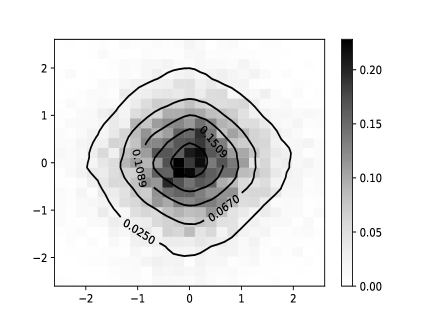
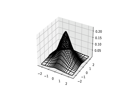
Example 2: $\alpha=(1.25,1.75)^{\texttt{T}}$, $\theta=(3.0,5.0)^{\texttt{T}}$, $\beta=(2.64,-4.49)^{\texttt{T}}$, $\rho=-0.70$

 
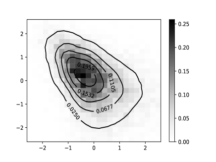
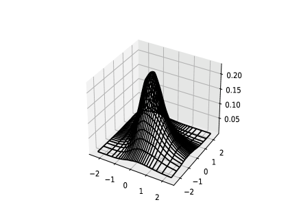
Example 3: $\alpha=(0.75,1.25)^{\texttt{T}}$, $\theta=(1.0,3.0)^{\texttt{T}}$, $\beta=(1.24,-2.74)^{\texttt{T}}$, $\rho=0.5$

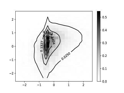
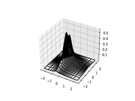
Figure 1: Contour graphs (left) and 3d graphs (right) of the PDFs for the three examples of gStdNTS distribution.

5.2 Parameter Estimation

For an empirical illustration, we consider daily prices of the Japanese Yen (JPY)-U.S. Dollar (USD) exchange rate and USD-valued Nikkei225 (N225) from January 2, 2020 to December 29, 2023. The USD-valued N225 prices are obtained by converting the original JPY-valued Nikkei225 levels into U.S. dollars using the JPY-USD exchange rate. Suppose $F(t)$ the process of the JPY-USD exchange rate, such that one JPY to $F(t)$ dollar, and $V(t)$ is the dollar-valued price process of the N225, that is $V(t)=S(t)F(t)$, where $S(t)$ is the N225 at time $t$. We estimate market parameters for daily log-returns on $V(t)$ and $F(t)$.

As (7) in Section 4, we set

$$(X(t))_{t\geq 0}\sim\textup{\rm gNTS}_{2}\left(\left(\begin{matrix}\alpha_{F}\\ \alpha_{V}\end{matrix}\right),\left(\begin{matrix}\theta_{F}\\ \theta_{V}\end{matrix}\right),\left(\begin{matrix}\beta_{F}\\ \beta_{V}\end{matrix}\right),\left(\begin{matrix}\mu_{F}\\ \mu_{V}\end{matrix}\right),\left(\begin{matrix}\sigma_{F}\\ \sigma_{V}\end{matrix}\right),\left(\begin{matrix}1&\rho\\ \rho&1\end{matrix}\right)\right)$$

with $X(t)=(X_{F}(t),X_{V}(t))^{\texttt{T}}$. We apply Proposition 3.3, we have

$$\left(\begin{matrix}X_{F}(\varDelta t)\\ X_{V}(\varDelta t)\end{matrix}\right)\stackrel{{\scriptstyle\mathrm{d}}}{{=}}\left(\begin{matrix}m_{F}\\ m_{V}\end{matrix}\right)+\left(\begin{matrix}s_{F}&0\\ 0&s_{V}\end{matrix}\right)\left(\begin{matrix}\Xi_{F}(1)\\ \Xi_{V}(1)\end{matrix}\right)$$ (9)

where $\Xi(1)=(\Xi_{F}(1),\Xi_{V}(1))^{\texttt{T}}$ and

$$\Xi\sim\textup{\rm gStdNTS}_{2}\left(\left(\begin{matrix}\alpha_{F}\\ \alpha_{V}\end{matrix}\right),\left(\begin{matrix}\theta_{\Xi,F}\\ \theta_{\Xi,V}\end{matrix}\right),\left(\begin{matrix}\beta_{\Xi,F}\\ \beta_{\Xi,V}\end{matrix}\right),\left(\begin{matrix}1&\rho\\ \rho&1\end{matrix}\right)\right)$$

with

$$\theta_{\Xi,n}=\theta_{n}\varDelta t^{\frac{2}{\alpha_{n}}},~{}~{}~{}\beta_{\Xi,n}=\frac{\beta_{n}\varDelta t^{\frac{2}{\alpha_{n}}}}{s_{n}},~{}~{}~{}m_{n}=\varDelta t\left(\mu_{n}+\frac{\alpha_{n}\beta_{n}}{2}\theta_{n}^{\frac{\alpha_{n}}{2}-1}\right),$$

and

$$s_{n}=\sqrt{\varDelta t\frac{\alpha_{n}}{2}\theta_{n}^{\frac{\alpha_{n}}{2}-1}\left(\left(\frac{2-\alpha_{n}}{2\theta_{n}}\right)\beta_{n}^{2}+\sigma_{n}^{2}\right)},$$

for $n\in\{F,V\}$. We estimate $(m_{F},m_{V})^{\texttt{T}}$ and $(s_{F},s_{V})^{\texttt{T}}$ by the sample mean and sample standard deviation of the FX rate return and the index return, respectively. Then we fit the gStdNTS parameters of $\Xi$ using maximum likelihood estimation with the PDF trained by CRealNVP transformations. We repeat this parameter fit process for the other pair of a FX rate & a market index such as British pound (GBP)-USD & Financial Times Stock Exchange 100 Index (FTSE), Euro currency (EUR)-USD & German stock Index (DAX), and Korean won (KRW)-USD & KOSPI200 Index (KS200). The estimation results are also presented in Table 2. The 2-dimensional histograms of the standardized log-returns of those 4 pairs are exhibited in Figure 2 together with the PDF contour map of gStdNTS distribution.

The estimated parameters for those four pairs of the FX rate and index returns are provided in the first row of Table 2. In the last column of the table, we present the Kolmogorov–Smirnov (K-S) statistic and $p$-values for the goodness of fit test for the 2 dimensional CDF of empirical data and gNTS model, respectively. In addition, the parameters of the NTS model are estimated as a benchmark model for the same data. In the NTS model, we assume that $X$ follows the NTS process and $X(\varDelta t)=m+\textrm{\rm diag}(s)\Xi(1)$ where $m=(m_{F},m_{V})^{\texttt{T}}$ and $s=(s_{F},s_{V})^{\texttt{T}}$ are the mean and standard deviation vectors, respectively, and $\Xi(1)$ is the standard NTS distributed with parameters $\left(\alpha,\theta,\beta_{\Xi},\left(\begin{smallmatrix}1&\rho\\ \rho&1\end{smallmatrix}\right)\right)$ with $\alpha\in(0,2)$, $\theta>0$, $\beta_{\Xi}=(\beta_{\Xi,F},\beta_{\Xi,V})^{\texttt{T}}$ and $\rho\in[-1,1]$. More details on parameter fitting are described in the literature, including Kim (2022). Comparing the K-S statistic, we see that the K-S statistic value for the NTS model is significantly larger than that of the gNTS model. According to the $p$-values, the estimated NTS distribution is rejected at the 5% significance level, while the gNTS model is not rejected. That is, the performance of the parameters fitted to the gNTS model is much better than that of the NTS model.

	mean	Standard Deviation	Model Parameters			K-S($p$-value)
			gStdNTS  paramters
JPY-USD	$m_{F}=-2.766\cdot 10^{-4}$	$s_{F}=5.812\cdot 10^{-3}$	$\alpha_{F}=1.0171$	$\theta_{\Xi,F}=1.365$	$\beta_{\Xi,F}=1.978\cdot 10^{-1}$	$0.0409$
N225	$m_{V}=9.847\cdot 10^{-5}$	$s_{V}=1.357\cdot 10^{-2}$	$\alpha_{V}=1.2300$	$\theta_{\Xi,V}=6.147\cdot 10^{-1}$	$\beta_{\Xi,V}=-2.188\cdot 10^{-1}$	$(0.1533)$
			$\rho=0.3134$
			stdNTS  paramters
			$\alpha=0.7644$	$\theta=1.0719$	$\beta_{\Xi,F}=1.735\cdot 10^{-1}$	$0.3071$
					$\beta_{\Xi,V}=-7.530\cdot 10^{-2}$	$(0.0000)$
			$\rho=0.3319$
			gStdNTS  paramters
GBP-USD	$m_{F}=-2.913\cdot 10^{-5}$	$s_{F}=6.211\cdot 10^{-3}$	$\alpha_{F}=1.2373$	$\theta_{\Xi,F}=1.332$	$\beta_{\Xi,F}=-1.940\cdot 10^{-1}$	$0.0288$
FTSE	$m_{V}=-4.320\cdot 10^{-6}$	$s_{V}=1.323\cdot 10^{-2}$	$\alpha_{V}=0.9258$	$\theta_{\Xi,V}=2.892\cdot 10^{-2}$	$\beta_{\Xi,V}=-1.534\cdot 10^{-2}$	$(0.7530)$
			$\rho=0.5366$
			stdNTS  paramters
			$\alpha=0.7195$	$\theta=0.9571$	$\beta_{\Xi,F}=5.590\cdot 10^{-2}$	$0.3143$
					$\beta_{\Xi,V}=-1.495\cdot 10^{-1}$	$(0.0000)$
			$\rho=0.4379$
			gStdNTS  paramters
EUR-USD	$m_{F}=-1.343\cdot 10^{-5}$	$s_{F}=4.911\cdot 10^{-3}$	$\alpha_{F}=1.3134$	$\theta_{\Xi,F}=4.341$	$\beta_{\Xi,F}=-1.414\cdot 10^{-1}$	$0.0294$
DAX	$m_{V}=2.065\cdot 10^{-4}$	$s_{V}=1.487\cdot 10^{-2}$	$\alpha_{V}=0.9193$	$\theta_{\Xi,V}=1.783\cdot 10^{-2}$	$\beta_{\Xi,V}=-3.488\cdot 10^{-3}$	$(0.6852)$
			$\rho=0.4192$
			stdNTS  paramters
			$\alpha=1.0756$	$\theta=1.0905$	$\beta_{\Xi,F}=6.332\cdot 10^{-2}$	$0.2947$
					$\beta_{\Xi,V}=-2.359\cdot 10^{-1}$	$(0.0000)$
			$\rho=0.3225$
			gStdNTS  paramters
KRW-USD	$m_{F}=-1.170\cdot 10^{-4}$	$s_{F}=5.929\cdot 10^{-3}$	$\alpha_{F}=1.1830$	$\theta_{\Xi,F}=1.090\cdot 10^{1}$	$\beta_{\Xi,F}=8.177\cdot 10^{-1}$	$0.0315$
KS200	$m_{V}=9.583\cdot 10^{-5}$	$s_{V}=1.567\cdot 10^{-2}$	$\alpha_{V}=1.3038$	$\theta_{\Xi,V}=4.696\cdot 10^{-3}$	$\beta_{\Xi,V}=-7.793\cdot 10^{-3}$	$(0.5658)$
			$\rho=0.6399$
			stdNTS  paramters
			$\alpha=0.7631$	$\theta=1.8986$	$\beta_{\Xi,F}=3.070\cdot 10^{-1}$	$0.3454$
					$\beta_{\Xi,V}=-3.070\cdot 10^{-1}$	$(0.0000)$
			$\rho=0.6185$

Table 2: Results of parameter estimation of gNTS model to the 4 pairs of foreign index returns and FX rate returns, respectively

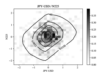
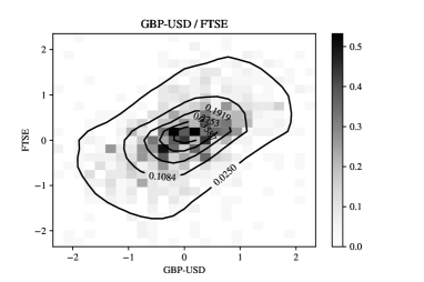
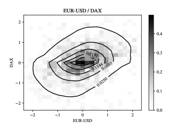
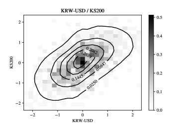
Figure 2: Histograms and contour graphs of the PDFs. The top-left is for JPY-USD and Nikkei 225 returns, the top-right is for GBP-USD and FTSE returns, the bottom-left is for EUR-USD and DAX returns and the bottom-right is for KRW-USD and KS200 returns.

5.3 Quanto Option Pricing

Suppose gNTS parameters of $X$ is given by (9). By proposition 3.2 (a), we have

$$(X(t))_{t\geq 0}\sim\textup{\rm gNTS}_{2}\left(\left(\begin{matrix}\alpha_{F}\\ \alpha_{V}\end{matrix}\right),\left(\begin{matrix}\theta_{F}\\ \theta_{V}\end{matrix}\right),\left(\begin{matrix}\beta_{F}\\ \beta_{V}\end{matrix}\right),\left(\begin{matrix}\mu_{F}\\ \mu_{V}\end{matrix}\right),\left(\begin{matrix}\sigma_{F}\\ \sigma_{V}\end{matrix}\right),\left(\begin{matrix}1&\rho\\ \rho&1\end{matrix}\right)\right)$$

where

$$\theta_{n}=\frac{\theta_{\Xi,n}}{\varDelta t^{\frac{2}{\alpha_{n}}}},~{}\beta_{n}=\frac{\beta_{\Xi,n}s_{n}}{\varDelta t^{\frac{2}{\alpha_{n}}}},~{}\mu_{n}=\frac{m_{n}}{\varDelta t}-\frac{\alpha_{n}\beta_{n}}{2}\theta_{n}^{\frac{\alpha_{n}}{2}-1},\sigma_{n}=\sqrt{\frac{2s_{n}^{2}\theta_{n}^{1-\frac{\alpha_{n}}{2}}}{\alpha_{n}\varDelta t}-\left(\frac{2-\alpha_{n}}{2\theta_{n}}\right)\beta_{n}^{2}}$$

for $n\in\{F,V\}$.

Let $r=(r_{F},r_{V})^{\texttt{T}}$ with $r_{F}=r_{d}-r_{f}$ and $r_{V}=r_{d}$ to simplify notations. There are infinitely many risk-neutral parameters $\hat{\theta}=(\hat{\theta}_{F},\hat{\theta}_{V})^{\texttt{T}}$ and $\hat{\beta}=(\hat{\beta}_{F},\hat{\beta}_{V})^{\texttt{T}}$ satisfying RN.2, which is equivalent to

$$\hat{\beta}_{n}=\hat{\theta}_{n}-\frac{\sigma_{n}^{2}}{2}-\left(\mu_{n}-r_{n}+\hat{\theta}_{n}^{\frac{\alpha_{n}}{2}}\right)^{\frac{2}{\alpha_{n}}},~{}~{}~{}\text{ for }n\in\{F,V\}.$$

To select one set of risk-neutral parameters, we try to find the parameter set which is as close to the physical parameters as possible. That is we find $\hat{\theta}^{*}=(\hat{\theta}^{*}_{F},\hat{\theta}^{*}_{V})^{\texttt{T}}$ and $\hat{\beta}^{*}=(\hat{\beta}^{*}_{F},\hat{\beta}^{*}_{V})^{\texttt{T}}$ close to the physical parameters $\theta$ and $\beta$ as follows:

$$(\hat{\theta}^{*}_{n},\hat{\beta}^{*}_{n})=\operatorname*{arg\,min}_{(\hat{\theta}_{n},\hat{\beta}_{n})}\sqrt{\left(\hat{\theta}_{n}-\theta_{n}\right)^{2}+\left(\hat{\beta}_{n}-\beta_{n}\right)^{2}},~{}~{}~{}\text{ for }n\in\{F,V\}.$$

Then we obtain

$$(X(t))_{t\geq 0}\sim\textup{\rm gNTS}_{2}\left(\left(\begin{matrix}\alpha_{F}\\ \alpha_{V}\end{matrix}\right),\left(\begin{matrix}\hat{\theta}^{*}_{F}\\ \hat{\theta}^{*}_{V}\end{matrix}\right),\left(\begin{matrix}\hat{\beta}^{*}_{F}\\ \hat{\beta}^{*}_{V}\end{matrix}\right),\left(\begin{matrix}\mu_{F}\\ \mu_{V}\end{matrix}\right),\left(\begin{matrix}\sigma_{F}\\ \sigma_{V}\end{matrix}\right),\left(\begin{matrix}1&\rho\\ \rho&1\end{matrix}\right)\right)$$

under the risk-neutral measure $\mathbb{Q}_{\hat{\theta}^{*},\hat{\beta}^{*}}$. Recall the quanto call option pricing formula (8) in Section 4, we consider the quanto call option with the time to maturity $T$, strike price $K$ and the fixed exchange rate $F_{\text{fix}}$. To calculate the quanto call price, we must know the distribution of $(X_{F}(T),X_{V}(T))^{\texttt{T}}$ for the time to maturity $T$. We apply Proposition 3.3 to $X$ under the risk-neutral measure $\mathbb{Q}_{\hat{\theta}^{*},\hat{\beta}^{*}}$, we obtain as follows:

$$\left(\begin{matrix}X_{F}(T)\\ X_{V}(T)\end{matrix}\right)\stackrel{{\scriptstyle\mathrm{d}}}{{=}}\left(\begin{matrix}\hat{m}_{F}\\ \hat{m}_{V}\end{matrix}\right)+\left(\begin{matrix}\hat{s}_{F}&0\\ 0&\hat{s}_{V}\end{matrix}\right)\left(\begin{matrix}\hat{\Xi}_{F}(1)\\ \hat{\Xi}_{V}(1)\end{matrix}\right)$$

with

$$\hat{\Xi}=(\hat{\Xi}_{F},\hat{\Xi}_{V})^{\texttt{T}}\sim\textup{\rm gStdNTS}_{2}\left(\left(\begin{matrix}\alpha_{F}\\ \alpha_{V}\end{matrix}\right),\left(\begin{matrix}\hat{\theta}_{\hat{\Xi},F}\\ \hat{\theta}_{\hat{\Xi},V}\end{matrix}\right),\left(\begin{matrix}\hat{\beta}_{\hat{\Xi},F}\\ \hat{\beta}_{\hat{\Xi},V}\end{matrix}\right),\left(\begin{matrix}1&\rho\\ \rho&1\end{matrix}\right)\right)$$

where

$$\hat{\theta}_{\hat{\Xi},n}=\hat{\theta}^{*}_{n}T^{\frac{2}{\alpha_{n}}},~{}~{}~{}\hat{\beta}_{\hat{\Xi},n}=\frac{\hat{\beta}^{*}_{n}T^{\frac{2}{\alpha_{n}}}}{s_{n}},~{}~{}~{}\hat{s}_{n}=\sqrt{\frac{\alpha_{n}T}{2}\left(\hat{\theta}^{*}_{n}\right)^{\frac{\alpha_{n}}{2}-1}\left(\left(\frac{2-\alpha_{n}}{2\hat{\theta}^{*}_{n}}\right)\left(\hat{\beta}^{*}_{n}\right)^{2}+\sigma_{n}^{2}\right)},$$

and

$$\hat{m}_{n}=T\left(r_{n}+\left(\hat{\theta}^{*}_{n}-\hat{\beta}^{*}_{n}-\frac{\sigma_{n}^{2}}{2}\right)^{\frac{\alpha_{n}}{2}}+\left(\frac{\alpha_{n}\hat{\beta}^{*}_{n}}{2\hat{\theta}^{*}_{n}}-1\right)\left(\hat{\theta}^{*}_{n}\right)^{\frac{\alpha_{n}}{2}}\right),~{}~{}~{}\text{ for }~{}~{}~{}n\in\{F,V\}.$$

Using the parameters, we continue option pricing of the equation (8):

$$E_{\mathbb{Q}_{\hat{\theta}^{*},\hat{\beta}^{*}}}\left[e^{-r_{d}T}F_{\text{fix}}(S(T)-K)^{+}\right]$$

$$=e^{-r_{d}T}F_{\text{fix}}E_{\mathbb{Q}_{\hat{\theta}^{*},\hat{\beta}^{*}}}\left[(S(0)\exp(\hat{m}_{F}+\hat{s}_{F}\hat{\Xi}_{F}(1)-\hat{m}_{V}-\hat{s}_{V}\hat{\Xi}_{V}(1))-K)^{+}\right].$$

Let

$$H(\hat{\Xi}(1))=\left(e^{\hat{s}_{F}\hat{\Xi}_{F}(1)-\hat{s}_{V}\hat{\Xi}_{V}(1)}-\frac{K}{S(0)e^{\hat{m}_{F}-\hat{m}_{V}}}\right)^{+}.$$

Then we have

$$E_{\mathbb{Q}_{\hat{\theta}^{*},\hat{\beta}^{*}}}\left[e^{-r_{d}T}F_{\text{fix}}(S(T)-K)^{+}\right]=e^{-r_{d}T}F_{\text{fix}}S(0)e^{\hat{m}_{F}-\hat{m}_{V}}E_{\mathbb{Q}_{\hat{\theta}^{*},\hat{\beta}^{*}}}\left[H(\hat{\Xi}(1))\right]$$

By the CRealNVP model, we set $\hat{\Xi}(1)=f^{-1}(Z|\Theta)$ with the standard normal $Z$, the inverse normalized flow $f^{-1}(z|\Theta)$, and the parameters $\Theta=\left(\alpha_{F},\alpha_{V},\hat{\theta}_{\hat{\Xi},F},\hat{\theta}_{\hat{\Xi},V},\hat{\beta}_{\hat{\Xi},F},\hat{\beta}_{\hat{\Xi},V},\rho\right)$. Then

$$E_{\mathbb{Q}_{\hat{\theta}^{*},\hat{\beta}^{*}}}\left[H(\hat{\Xi}(1))\right]=E_{\mathbb{Q}_{\hat{\theta}^{*},\hat{\beta}^{*}}}\left[H\left(f^{-1}(Z|\Theta)\right)\right]=\iint H\left(f^{-1}(z|\Theta)\right)p_{Z}(z)dz,$$

where $p_{Z}(z)$ the PDF of the 2-dimensional standard normal distribution. The double integral can be approximated by a numerical integration.

	$S(0)$	$F_{\text{fix}}$	$r_{f}$
JPY-USD/N225	$17047.4$	$7.071\cdot 10^{-3}$	$-0.1\%$
GBP-USD/FTSE	$7733.20$	$1.273$	$5.25\%$
EUR-USD/DAX	$16751.6$	$1.107$	$4.5\%$
KRW-USD/KS200	$357.990$	$7.826\cdot 10^{-4}$	$3.5\%$

Table 3: Market information on December 29, 2023. $S(0)$, $F_{\text{fix}}$, and $r_{f}$ mean the foreign index, FX rate, and foreign risk-free rate with respect to the 4 pairs of the examples, respectively

For example, we calculate $(\hat{m}_{F},\hat{m}_{V})^{\texttt{T}}$, $(\hat{s}_{F},\hat{s}_{V})^{\texttt{T}}$, $(\hat{\theta}_{\hat{\Xi},F},\hat{\theta}_{\hat{\Xi},V})^{\texttt{T}}$ and $(\hat{\beta}_{\hat{\Xi},F},\hat{\beta}_{\hat{\Xi},V})^{\texttt{T}}$ for $T\in\{1/52(1$-week$)$, $2/52(2$-weeks$)$, $3/52(3$-weeks$)$, $4/52(4$-weeks$)\}$ based on the estimated parameters in Table 2 for the 4 cases (JPY-USD/N225, GBP-USD/FTSE, EUR-USD/DAX, KRW-USD/KS200). In this calculation, we set $r_{d}=5.5\%$ which is the U.S standard rate (Federal Fund Rate), and we set $r_{f}$ in $\{-0.1\%$, $5.25\%$, $4.5\%$, $3.5\%\}$ which are standard rates of Japan, U.K., European union, and Korea, respectively, on December 2023 (See Table 3). The risk neutral parameters based on this calculation are presented in Table 4. Moreover, the values of $S(0)$ and $F_{\text{fix}}$ are presented in Table 3 which are observed on December 29, 2023.

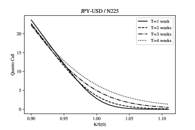
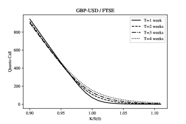
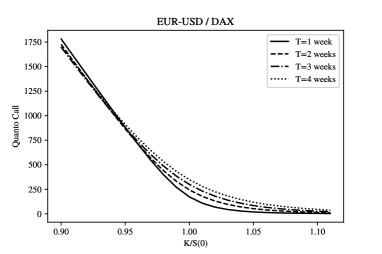
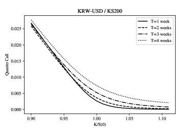
Figure 3: Quanto Call Prices. The top-left is for JPY-USD/N225, the top-right is for GBP-USD/FTSE, the bottom-left is for EUR-USD/DAX and the bottom-right is for KRW-USD/KS200 returns.

The quanto call option prices for the 4 cases with the risk-neutral parameters in Table 4 for time to maturities 1-4 weeks are calculated and presented in Figure 3. Since the index prices are all different, we use the moneyness $M=K/S(0)$ instead of the strike price $K$, and change the function $H$ to

$$H(\hat{\Xi}(1))=\left(e^{\hat{s}_{F}\hat{\Xi}_{F}(1)-\hat{s}_{V}\hat{\Xi}_{V}(1)}-Me^{-\hat{m}_{F}+\hat{m}_{V}}\right)^{+}.$$

For the reason, the $x$-axes of the 4 plates of Figure 3 present the moneyness $K/S(0)$.

	$T$ (week)	mean	Standard Deviation	Risk-neutral gStdNTS parameters
JPY-USD	1	$\hat{m}_{F}=9.936\cdot 10^{-4}$	$\hat{s}_{F}=1.291\cdot 10^{-2}$	$\hat{\theta}_{\hat{\Xi},F}=3.040\cdot 10^{1}$	$\hat{\beta}_{\hat{\Xi},F}=3.889$
N225		$\hat{m}_{V}=-4.661\cdot 10^{-4}$	$\hat{s}_{V}=2.993\cdot 10^{-2}$	$\hat{\theta}_{\hat{\Xi},V}=8.001$	$\hat{\beta}_{\hat{\Xi},V}=-1.405$
	2	$\hat{m}_{F}=1.987\cdot 10^{-3}$	$\hat{s}_{F}=1.825\cdot 10^{-2}$	$\hat{\theta}_{\hat{\Xi},F}=1.188\cdot 10^{2}$	$\hat{\beta}_{\hat{\Xi},F}=1.074\cdot 10^{1}$
		$\hat{m}_{V}=-9.322\cdot 10^{-4}$	$\hat{s}_{V}=4.232\cdot 10^{-2}$	$\hat{\theta}_{\hat{\Xi},V}=2.470\cdot 10^{1}$	$\hat{\beta}_{\hat{\Xi},V}=-3.067$
	3	$\hat{m}_{F}=2.981\cdot 10^{-3}$	$\hat{s}_{F}=2.236\cdot 10^{-2}$	$\hat{\theta}_{\hat{\Xi},F}=2.637\cdot 10^{2}$	$\hat{\beta}_{\hat{\Xi},F}=1.947\cdot 10^{1}$
		$\hat{m}_{V}=-1.398\cdot 10^{-3}$	$\hat{s}_{V}=5.183\cdot 10^{-2}$	$\hat{\theta}_{\hat{\Xi},V}=4.775\cdot 10^{1}$	$\hat{\beta}_{\hat{\Xi},V}=-4.841$
	4	$\hat{m}_{F}=3.974\cdot 10^{-3}$	$\hat{s}_{F}=2.581\cdot 10^{-2}$	$\hat{\theta}_{\hat{\Xi},F}=4.643\cdot 10^{2}$	$\hat{\beta}_{\hat{\Xi},F}=2.969\cdot 10^{1}$
		$\hat{m}_{V}=-1.864\cdot 10^{-3}$	$\hat{s}_{V}=5.985\cdot 10^{-2}$	$\hat{\theta}_{\hat{\Xi},V}=7.623\cdot 10^{1}$	$\hat{\beta}_{\hat{\Xi},V}=-6.694$
GBP-USD	1	$\hat{m}_{F}=-4.535\cdot 10^{-5}$	$\hat{s}_{F}=1.367\cdot 10^{-2}$	$\hat{\theta}_{\hat{\Xi},F}=1.707\cdot 10^{1}$	$\hat{\beta}_{\hat{\Xi},F}=-1.097$
FTSE		$\hat{m}_{V}=5.886\cdot 10^{-4}$	$\hat{s}_{V}=2.906\cdot 10^{-2}$	$\hat{\theta}_{\hat{\Xi},V}=8.747\cdot 10^{-1}$	$\hat{\beta}_{\hat{\Xi},V}=-1.692\cdot 10^{-1}$
	2	$\hat{m}_{F}=-9.069\cdot 10^{-5}$	$\hat{s}_{F}=1.933\cdot 10^{-2}$	$\hat{\theta}_{\hat{\Xi},F}=5.235\cdot 10^{1}$	$\hat{\beta}_{\hat{\Xi},F}=-2.378$
		$\hat{m}_{V}=1.177\cdot 10^{-3}$	$\hat{s}_{V}=4.109\cdot 10^{-2}$	$\hat{\theta}_{\hat{\Xi},V}=3.910$	$\hat{\beta}_{\hat{\Xi},V}=-5.347\cdot 10^{-1}$
	3	$\hat{m}_{F}=-1.360\cdot 10^{-4}$	$\hat{s}_{F}=2.368\cdot 10^{-2}$	$\hat{\theta}_{\hat{\Xi},F}=1.008\cdot 10^{2}$	$\hat{\beta}_{\hat{\Xi},F}=-3.740$
		$\hat{m}_{V}=1.766\cdot 10^{-3}$	$\hat{s}_{V}=5.033\cdot 10^{-2}$	$\hat{\theta}_{\hat{\Xi},V}=9.389$	$\hat{\beta}_{\hat{\Xi},V}=-1.048$
	4	$\hat{m}_{F}=-1.814\cdot 10^{-4}$	$\hat{s}_{F}=2.734\cdot 10^{-2}$	$\hat{\theta}_{\hat{\Xi},F}=1.605\cdot 10^{2}$	$\hat{\beta}_{\hat{\Xi},F}=-5.157$
		$\hat{m}_{V}=2.354\cdot 10^{-3}$	$\hat{s}_{V}=5.812\cdot 10^{-2}$	$\hat{\theta}_{\hat{\Xi},V}=1.748\cdot 10^{1}$	$\hat{\beta}_{\hat{\Xi},V}=-1.690$
EUR-USD	1	$\hat{m}_{F}=1.339\cdot 10^{-4}$	$\hat{s}_{F}=1.081\cdot 10^{-2}$	$\hat{\theta}_{\hat{\Xi},F}=4.800\cdot 10^{1}$	$\hat{\beta}_{\hat{\Xi},F}=-6.043\cdot 10^{-1}$
DAX		$\hat{m}_{V}=3.291\cdot 10^{-4}$	$\hat{s}_{V}=3.279\cdot 10^{-2}$	$\hat{\theta}_{\hat{\Xi},V}=5.525\cdot 10^{-1}$	$\hat{\beta}_{\hat{\Xi},V}=-8.136\cdot 10^{-2}$
	2	$\hat{m}_{F}=2.678\cdot 10^{-4}$	$\hat{s}_{F}=1.529\cdot 10^{-2}$	$\hat{\theta}_{\hat{\Xi},F}=1.379\cdot 10^{2}$	$\hat{\beta}_{\hat{\Xi},F}=-1.228$
		$\hat{m}_{V}=6.581\cdot 10^{-4}$	$\hat{s}_{V}=4.637\cdot 10^{-2}$	$\hat{\theta}_{\hat{\Xi},V}=2.496$	$\hat{\beta}_{\hat{\Xi},V}=-2.599\cdot 10^{-1}$
	3	$\hat{m}_{F}=4.017\cdot 10^{-4}$	$\hat{s}_{F}=1.872\cdot 10^{-2}$	$\hat{\theta}_{\hat{\Xi},F}=2.557\cdot 10^{2}$	$\hat{\beta}_{\hat{\Xi},F}=-1.859$
		$\hat{m}_{V}=9.872\cdot 10^{-4}$	$\hat{s}_{V}=5.679\cdot 10^{-2}$	$\hat{\theta}_{\hat{\Xi},V}=6.031$	$\hat{\beta}_{\hat{\Xi},V}=-5.127\cdot 10^{-1}$
	4	$\hat{m}_{F}=5.356\cdot 10^{-4}$	$\hat{s}_{F}=2.162\cdot 10^{-2}$	$\hat{\theta}_{\hat{\Xi},F}=3.963\cdot 10^{2}$	$\hat{\beta}_{\hat{\Xi},F}=-2.495$
		$\hat{m}_{V}=1.316\cdot 10^{-3}$	$\hat{s}_{V}=6.557\cdot 10^{-2}$	$\hat{\theta}_{\hat{\Xi},V}=1.128\cdot 10^{1}$	$\hat{\beta}_{\hat{\Xi},V}=-8.302\cdot 10^{-1}$
KRW-USD	1	$\hat{m}_{F}=2.992\cdot 10^{-4}$	$\hat{s}_{F}=1.307\cdot 10^{-2}$	$\hat{\theta}_{\hat{\Xi},F}=1.570\cdot 10^{2}$	$\hat{\beta}_{\hat{\Xi},F}=6.232$
KS200		$\hat{m}_{V}=8.016\cdot 10^{-5}$	$\hat{s}_{V}=3.460\cdot 10^{-2}$	$\hat{\theta}_{\hat{\Xi},V}=5.286\cdot 10^{-2}$	$\hat{\beta}_{\hat{\Xi},V}=-4.584\cdot 10^{-2}$
	2	$\hat{m}_{F}=5.985\cdot 10^{-4}$	$\hat{s}_{F}=1.848\cdot 10^{-2}$	$\hat{\theta}_{\hat{\Xi},F}=5.069\cdot 10^{2}$	$\hat{\beta}_{\hat{\Xi},F}=1.423\cdot 10^{1}$
		$\hat{m}_{V}=1.603\cdot 10^{-4}$	$\hat{s}_{V}=4.893\cdot 10^{-2}$	$\hat{\theta}_{\hat{\Xi},V}=1.531\cdot 10^{-1}$	$\hat{\beta}_{\hat{\Xi},V}=-9.388\cdot 10^{-2}$
	3	$\hat{m}_{F}=8.977\cdot 10^{-4}$	$\hat{s}_{F}=2.263\cdot 10^{-2}$	$\hat{\theta}_{\hat{\Xi},F}=1.006\cdot 10^{3}$	$\hat{\beta}_{\hat{\Xi},F}=2.305\cdot 10^{1}$
		$\hat{m}_{V}=2.405\cdot 10^{-4}$	$\hat{s}_{V}=5.992\cdot 10^{-2}$	$\hat{\theta}_{\hat{\Xi},V}=2.851\cdot 10^{-1}$	$\hat{\beta}_{\hat{\Xi},V}=-1.428\cdot 10^{-1}$
	4	$\hat{m}_{F}=1.197\cdot 10^{-3}$	$\hat{s}_{F}=2.613\cdot 10^{-2}$	$\hat{\theta}_{\hat{\Xi},F}=1.636\cdot 10^{3}$	$\hat{\beta}_{\hat{\Xi},F}=3.247\cdot 10^{1}$
		$\hat{m}_{V}=3.207\cdot 10^{-4}$	$\hat{s}_{V}=6.919\cdot 10^{-2}$	$\hat{\theta}_{\hat{\Xi},V}=4.433\cdot 10^{-1}$	$\hat{\beta}_{\hat{\Xi},V}=-1.922\cdot 10^{-1}$

Table 4: Risk-neural parameters minimize the distance from the historically estimated physical parameters for the 4 pairs of examples, respectively.

6 Conclusion

We have discussed a method to pricing European quanto options based on the gNTS model. The gNTS process captures both the fat-tail property and asymmetric dependence between returns of a FX rate and a corresponding foreign index. Different from the NTS process, the gNTS process allows different subordinators to the foreign index and FX return distributions, respectively, and it describes different volatility characteristic for the FX rate and foreign index, that is not captured by the NTS model.

Since the gNTS  does not have a simple analytic form of distribution, we use the CRealNVP model to find the PDF of gNTSprocess. We construct the CRealNVP model for the gStdNTS process in this study and train the model using the training set generated by Monte-Carlo simulation of the gStdNTS process. The gNTS process can be decomposed by the mean, standard deviation and gStdNTS process. We empirically fit the gStdNTS process parameters to the 4 pairs of FX rate and foreign index data: USD-JPY/N225, USD-GBP/FTSE, USD-EUR/DAX, and UDS-KRW/KS200. According to the K-S test in this investigation, the parameter estimation for gNTS model performs better than that for the NTS model which is the benchmark model.

A risk-neutral measure of gNTSmodel is obtained by applying Sato’s theorem and Girsanov’s theorem for the time changed Borwnian motion model. Since there are infinitely many risk-neutral measures in gNTS model, we select one risk-neutral measure whose parameter set has the smallest distance from the parameter set of the physical measure. This method was applied for the 4 example pairs of the empirical data, and the risk neutral parameters are obtained for each case. Using the risk-neutral parameters, we successfully calculate prices of the example quanto option for the 4 pairs of FX rates and foreign market indexes.

We conclude that the distribution of gNTS process successfully obtained by CRealNVP model. Using this method, we can fit the gNTS process to the empirical data efficiently. Moreover, we can find the risk-neutral measure of the gNTS model, and calculate price of quanto option using the CRealNVP model with the risk-neutral parameters.

References

• Anand et al. (2016) Anand, A., Li, T., Kurosaki, T., and Kim, Y. S. (2016). Foster-Hart optimal portfolios. Journal of Banking and Finance, 68, 117–130.
• Baxter and Rennie (1996) Baxter, M. and Rennie, A. (1996). Financial Calculus: An Introduction to Derivative Pricing. Cambridge University Press.
• Black and Scholes (1973) Black, F. and Scholes, M. (1973). The pricing of options and corporate liabilities. The Journal of Political Economy, 81(3), 637–654.
• Dinh et al. (2016) Dinh, L., Sohl-Dickstein, J., and Bengio, S. (2016). Density estimation using RealNVP. ArXiv preprint, arXiv:1605.08803.
• Goodfellow et al. (2014) Goodfellow, I., Pouget-Abadie, J., nad B. Xu, M. M., Warde-Farley, D., Ozair, S., Courville, A., and Bengio, Y. (2014). Generative adversarial networks. ArXiv preprint, arXiv:1406.2661.
• Kim et al. (2022) Kim, H.-G., Kwon, S.-J., Kim, J.-H., and Huh, J. (2022). Pricing path-dependent exotic options with flow-based generative networks. Applied Soft Computing, 124, 109049. URL https://doi.org/10.1016/j.asoc.2022.109049.
• Kim (2022) Kim, Y. (2022). Portfolio optimization and marginal contribution to risk on multivariate normal tempered stable model. Annals of Operations Research, 312, 853––881.
• Kim et al. (2015) Kim, Y., Lee, J., Mittnik, S., and Park, J. (2015). Quanto option pricing in the presence of fat tails and asymmetric dependence. Journal of Econometrics, 187(2), 512 – 520.
• Kim and Lee (2007) Kim, Y. and Lee, J. H. (2007). The relative entropy in CGMY processes and its applications to finance. Mathematical Methods of Operations Research, 66(2), 327–338.
• Kim (2005) Kim, Y. S. (2005). The modified tempered stable processes with application to finance. Ph.D thesis, Sogang University.
• Kim et al. (2023) Kim, Y. S., Kim, H., Choi, J., and Fabozzi, F. J. (2023). Multi-asset option pricing using normal tempered stable processes with stochastic correlation. The Journal of Derivatives, 30(3), 42–64.
• Kim and Volkmann (2013) Kim, Y. S. and Volkmann, D. (2013). NTS copula and finance. Applied Mathematics Letters, 26, 676–680.
• Kingma and Welling (2013) Kingma, D. and Welling, M. (2013). Auto-encoding variational bayes. ArXiv preprint, arXiv:1312.6114.
• Klebaner (2005) Klebaner, F. C. (2005). Introduction to Stochastic Calculus with Applications. Imperial College Press, 2nd ed.
• Kurosaki and Kim (2018) Kurosaki, T. and Kim, Y. S. (2018). Foster-Hart optimization for currency portfolio. Studies in Nonlinear Dynamics & Econometrics, 23(2), Published Online.
• Naaman (2021) Naaman, M. (2021). On the tight constant in the multivariate dvoretzky–kiefer–wolfowitz inequality. Statistics & Probability Letters, 173, 109088. URL https://www.sciencedirect.com/science/article/pii/S016771522100050X.
• Sato (1999) Sato, K. (1999). Lévy Processes and Infinitely Divisible Distributions. Cambridge University Press.