Using AI libraries for Incompressible Computational Fluid Dynamics

Abstract

Recently, there has been a huge effort focused on developing highly efficient open source libraries to perform Artificial Intelligence (AI) related computations on different computer architectures (for example, CPUs, GPUs and new AI processors). This has not only made the algorithms based on these libraries highly efficient and portable between different architectures, but also has substantially simplified the entry barrier to develop methods using AI. Here, we present a novel methodology to bring the power of both AI software and hardware into the field of numerical modelling by repurposing AI methods, such as Convolutional Neural Networks (CNNs), for the standard operations required in the field of the numerical solution of Partial Differential Equations (PDEs). The aim of this work is to bring the high performance, architecture agnosticism and ease of use into the field of the numerical solution of PDEs. We use the proposed methodology to solve the advection-diffusion equation, the non-linear Burgers equation and incompressible flow past a bluff body. For the latter, a convolutional neural network is used as a multigrid solver in order to enforce the incompressibility constraint. We show that the presented methodology can solve all these problems using repurposed AI libraries in an efficient way, and presents a new avenue to explore in the development of methods to solve PDEs and Computational Fluid Dynamics problems with implicit methods.

1 Introduction

In recent years, Artificial intelligence (AI) has provided the ability to address challenges that previously could not be solved by classical means, such as the identification of images, spam control, predictive writing and developing self-driving cars [1]. This huge success has encouraged not only the development of better and more sophisticated methods within the field of AI, but also the development of open source libraries devoted to simplify the entrance to and the use of AI. Some of the most popular libraries, such as PyTorch [2], TensorFlow [3], scikit-learn [4], XGBoost [5] and JAX [6], are maintained by large companies yet are also contributed to by their associated communities. These libraries are highly optimised, easy to use, well documented, deployable on different hardware architectures and are, consequently, widely used. In order to deploy these libraries on different architectures, the user needs only to make minimal changes to the code. For codes written in C++ and Fortran, for example, this is not the case: programmers have to grapple with rewriting code or writing additional code in largely unfamiliar languages in order to exploit the benefits of GPUs. Machine learning libraries have also been written so that any platform-specific code is hidden from the user.

As well as driving the continued development of accessible platform-independent code, AI has also been the inspiration behind the design of a number of specific architectures that are highly optimised for certain tasks commonly performed in AI, such as dense matrix-vector multiplication. Also known as AI chips and AI accelerators, new AI processors being unveiled include Google’s Tensor Processing Units (TPUs) [7], Cerebras’s CS-2 [8] and Graphcore’s Intelligence Processing Units (IPU) [9]. When designing these new processors, companies are looking to reduce the large energy overheads seen in large clusters of CPUs and GPUs. For example, with nearly 1 million cores on a single chip, Cerebras’s CS-2 has been reported to be up to 10 times as energy efficient as some other GPUs [10]. This is becoming particularly important as we may not be able to afford to run large petascale or exascale simulations on current CPU clusters due to the need to reduce our energy usage and the associated impact on our planet [11]. The approach proposed here, of numerically solving Partial Differential Equations (PDEs) using methods in machine-learning libraries, therefore brings the use of these new AI processors closer and makes the solution of the large systems of equations formed by the discretisation of PDEs, potentially more environmentally friendly.

During the last three years, scientists have begun to exploit GPUs and TPUs for scientific computation. Matrix-vector multiplications can be performed much faster, and this has been done for reconstruction of magnetic resonance images [12, 13], the dynamics of many-body quantum systems [14], quantum chemistry [15]. Many independent processes can also be run efficiently on GPUs and TPUs, such as Monte Carlo simulations, and this has been done for option pricing and hedging [16]. Of particular relevance to our work are two articles which solve computational fluid dynamics problems using convolutional operations to represent finite difference discretisations [17, 18]. Zhao et al. [17] code an explicit high-order finite-difference discretisation of the Navier-Stokes equations through TensorFlow. A constrained interpolation profile scheme is used to solve the advection term and preconditioned conjugate gradient method is used to solve the Poisson equation. A number of 2D test cases are used for demonstration, including lid-driven cavity flow and flow past a cylinder. The authors obtain good qualitative agreement when validating their results against the literature. For numbers of grid points larger than $25\,000$ and up to just over $600\,000$, their proposed method is over 10 times faster (running on GPUs) than their original Fortran-based code (running on CPUs). Wang et al. [18] present a similar idea, also using TensorFlow, to implement a finite-difference discretisation of the variable-density Navier-Stokes equations. They deploy their models on TPUs and achieve good weak and strong scaling. The 2D and 3D Taylor-Green vortex benchmarks are used for validation, and the expected convergence rates are found as the spatial resolution is increased (using up to 10⁹ grid points. The capability to model turbulent flows is demonstrated by modelling a planar jet, the results of which show good statistical agreement with reference solutions.

Here, we propose a way of developing CFD software based on methods and techniques available in AI libraries, which can simplify its development by repurposing the AI libraries to perform the same operations that CFD software would normally do. In this way, for example, a convolutional neural network (CNN) can be repurposed to become a structured multigrid solver, where the convolution operator is equivalent to the restriction operator and the smoothing steps are performed using a neural network. By repurposing readily available software, we expect that the development of CFD can benefit in at least three areas: (i) deployment to different computer architectures (such as TPUs and new AI processors with distributed memory) will be more efficient, and the resulting code will be specifically optimised for that architecture; (ii) reduction of the implementation time and lowering of the entry barrier by making the code more “high-level” than current CFD software implementations. We agree with Beck and Kurz [19], that the approach taken here and in Zhao et al. [17], Wang et al. [18] can be (iii) easily combined with trained neural networks, either of physics-informed or physics-aware approaches or for including subgrid-scale models based on neural networks, leading to a seamless integration machine-learning models with fluid solvers. In fact, some researchers have used matrices that are related (within a multiplicative constant) to finite difference discretisations in physics-informed approaches [20]. However, in the physics-informed approach, a neural network is trained albeit with a loss that is constrained to obey particular physical laws, so the discretisation will not be satisfied exactly.

Developed to solve systems of discretised PDEs, the idea behind multigrid methods is that it is beneficial to transfer information between solutions at different resolutions. In geometric multigrid, the discretised equations are solved on a hierarchy of grids, passing the residual from one level to another in order to increase the convergence rate [21, 22, 23]. This concept has similarities with a family of encoder-decoder neural networks, which includes the U-Net [24]. In the encoder of a U-Net, an image is repeatedly downsampled enabling the network to learn progressively larger-scale behaviour. The decoder acts in reverse and increases the resolution of the feature maps. In addition, there are skip connections which link layers of similar resolution in the encoder and decoder. As the decoder is reconstructing the images, the skip connections give it direct access to information at the same resolution from the encoder, which is thought to improve convergence of the network. Although there are examples of using ideas from multigrid to benefit neural networks [25], we believe our paper is the first implementation of a multigrid method using a U-Net architecture.

This paper is the first in a set of related papers [26, 27, 28, 29, 30] on solving discretised systems with (untrained) neural networks. After benchmarking and validating the approach for single-phase flows in this paper, have extended the idea to model more complex physics, including neutron diffusion [26] and multiphase flows [27]. To use higher-order finite element schemes, we have introduced a new finite element method which has the same stencil for every node [28]. We are also developing the method to model flooding through the shallow water equations [29]. We have also incorporated this approach in a geoscientific inversion problem, which predicts a potential from a prior conductivity field, obtained from a generative AI model. Observations of potential are assimilated and improved estimates of the conductivity (and therefore the subsurface) are obtained [30]. The assimilation process uses the backpropagation functions within the machine learning libraries applied to the forward model which is expressed as a neural network.

The structure of the remaining paper is as follows. The methods involved in expressed discretised systems of PDEs as neural networks, and solving these systems also with neural networks is explained in Section 2. Results are presented in Section 3 and a discussion follows in Section 4.

2 Methods

2.1 Multigrid methods based on CNNs

For incompressible flow, the most computationally expensive part of the simulation is the resolution of the linear system of equations. Multigrid methods produce to the fastest solvers for these large systems of equations. The similarities between CNN and multigrid solvers are striking, and work is already underway to use trained CNNs to solve systems of discrete equations, from CFD, using multigrid methods, see [31].

A geometric multigrid method works by creating a hierarchy of nested meshes and solving the equations at all levels, using the coarser meshes to correct the solution of the finer meshes. Multigrid methods consist of three basic operations: (i) Smoothing: typically a couple of iterations of a linear solver such as Jacobi or Gauss-Seidel are performed; (ii) Restriction: interpolation of the residual from a given mesh to a coarser mesh; (iii) Prolongation: extrapolation of the error correction from a coarse mesh to a finer mesh. A multigrid iteration or cycle consists of performing the following steps:

1. Smooth $\eta$ times;

2. Compute residual and restrict to a coarser mesh;

3. Smooth $\eta$ times;

4. Repeat steps (2) and (3) until reaching the coarsest mesh desired;

5. Solve exactly the system;

6. Prolongate from coarse mesh and correct the solution from the finer mesh;

7. Smooth $\phi$ times;

8. Repeat steps (6) and (7) until reaching the finest mesh.

In this work, we use the simplest multigrid (MG) method often referred to as a sawtooth-cycle [32], but restricting from the finest to the coarsest mesh and then prolongate and smooth at each mesh level in steps from coarsest to finest resolution each multigrid iteration, see Figure 1.

Here we effectively send the equation residuals onto the different grid levels, starting from the coarsest grid level we perform alternating Jacobi relaxation of the solution followed by prolongation of the resulting solution to the next grid level up in the hierarchy. The approach uses the coarsening levels of the CNN and in this case a single convolutional filter is used to represent the matrix equation. Here we have labelled on the left the weights of the neural network which can be effected by a single filter between the layers. The filters change between the layers, when we apply Jacobi relaxation, because the grid spacing $\Delta x$ changes between the layers.

We have indicated, only on the output layer, how biases (middle row left picture of Figure 1) can be applied to the neurons to effect the source problem associated with the Jacobi relaxation. However, biases are not consistent with the feed-forward propagation of the neural network information i.e. placing residuals from previous convolutional layers into the biases. Thus we use in our implementation layer skipping to send these residuals from the coarsening action of the convolutional neural network in a method akin to the use of the U-net (a commonly used neural network, see [24]), see Figure 1 bottom row left diagram. This figure shows the structure of the neural network for one multigrid cycle (we use 1MG to denote the resulting neural network). Several 1MG networks, or multigrid cycles, can be strung together to form an overall multigrid method, see figure bottom row left diagram Figure 1.

Assuming we are solving $Ax=s$, the Jacobi smoother or relaxation method can be defined as a Jacobi iteration:

$$x^{new}_{i}=\frac{1}{a_{ii}}\left(\sum_{j}a_{ij}x^{old}_{j}\;\;\;+s_{i}\right).$$ (1)

Now applying relaxation $x_{i}=\alpha x^{new}_{i}+(1-\alpha)x^{old}_{i}$ results in:

$$x_{i}=\alpha x^{new}_{i}+(1-\alpha)\frac{1}{a_{ii}}\left(\sum_{j}a_{ij}x^{old}_{j}\;\;\;+s_{i}\right).$$ (2)

Here, we use $\alpha=1$ for the relaxation coefficient, although, in general, $\alpha\in(0,2]$. Thus

$$x_{i}=\sum_{j}b_{ij}x^{old}_{j}\;\;\;+c_{i}$$ (3)

in which

$$b_{ij} = \alpha\frac{1}{a_{ii}}a_{ij}\;\;\;{\text{if}}\;\;\;i\neq j,$$ (4)

$$b_{ii} = 1,$$ (5)

$$\text{and }c_{i} = \alpha\left(\frac{1}{a_{ii}}\right)s_{i},$$ (6)

where $c_{i}$ is the bias, realised by CNN layer skipping, see Figure 1, bottom left diagram. Thus $w_{ij}=b_{ij}$ are the weights of the convolutional filter.

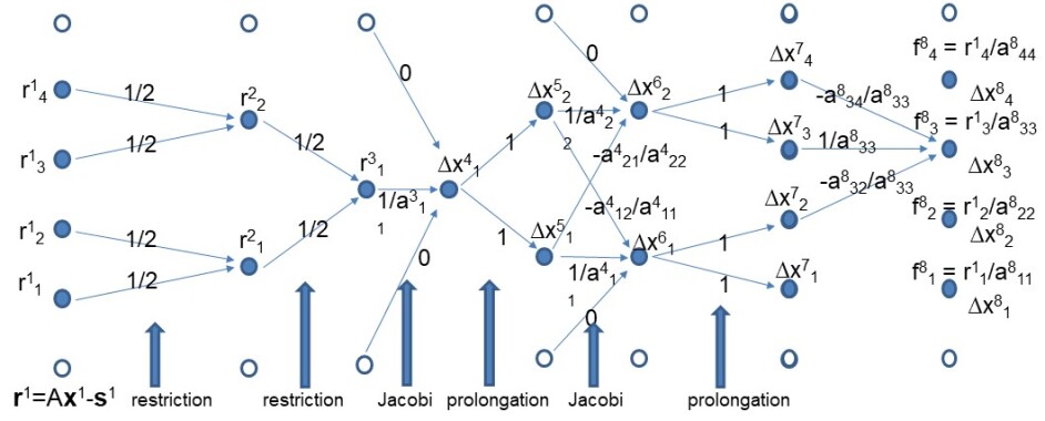
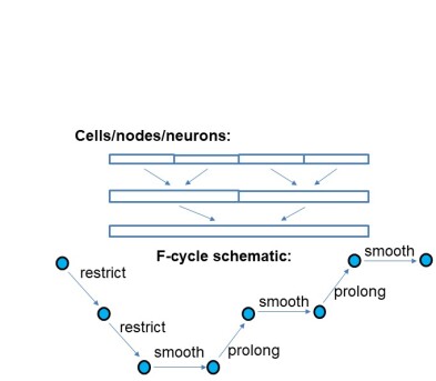
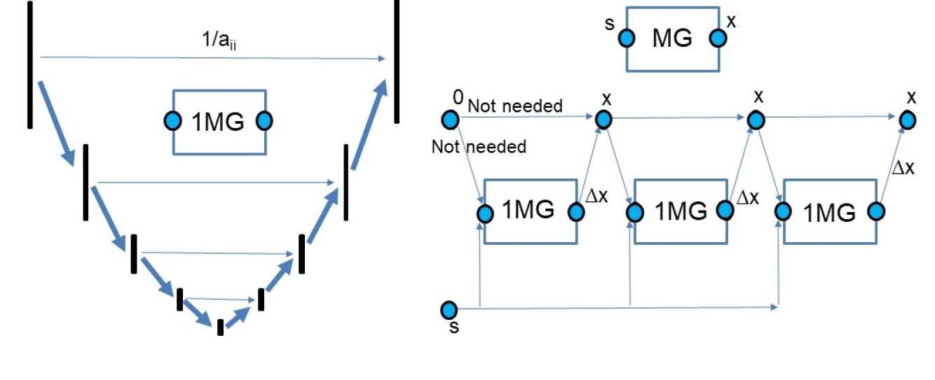
Figure 1: Schematic showing the how the CNNs are repurposed to produce a multigrid method. Top row left: How a 1D CNN multigrid method works with biases $f$. Top right: The four 1D cells that have two levels of coarsening and the schematic showing how this multigrid method works. Bottom row left: Schematic showing how one multigrid cycle works using layer skipping to pass the residual between the layers akin the U-net — this is a better alternative to using biases for the residuals. Bottom row right: Schematic showing how three multigrid cycles are brought together to form an overall matrix solution method.

2.2 Advection-diffusion solution

The advection-diffusion equation solved here is given by:

$$\frac{\partial T}{\partial t}+u\frac{\partial T}{\partial x}+v\frac{\partial T}{\partial y}+\sigma T-\nu\nabla^{2}T=s\,,$$ (7)

in which $T$ is a scalar concentration field, $(u,v)$ are the advection velocities, $\sigma$ is an absorption term, $\nu$ the constant diffusivity and $s$ the source. In the advection-diffusion simulations presented here, $\sigma=s=0$ although none zero values of $\sigma$ will be used for the momentum equations, Equations 22.

For simplicity we write out the discretisation only for a simple central difference advection scheme, second-order diffusion scheme and second order in time. We also use a first order upwind advection scheme in some of the applications and more complex central difference discretisations of advection and diffusion for the flow past a bluff body, see appendix. For a regular grid ($\Delta x=\Delta y$) and an advection velocity of $(u,v)=(1,1)$, the spatial derivatives can be written as

$$\left(\frac{\partial T}{\partial x}\right)_{\ell,\,m} \approx \frac{T_{\ell+1,\,m}-T_{\ell-1,\,m}}{2\Delta x}\,,$$ (8)

$$\left(\frac{\partial T}{\partial y}\right)_{\ell,\,m} \approx \frac{T_{\ell,\,m+1}-T_{\ell,\,m-1}}{2\Delta x}\,,$$ (9)

$$-\left(\frac{\partial^{2}T}{\partial x^{2}}\right)_{\ell,\,m} \approx \frac{-T_{\ell+1,\,m}+2T_{\ell,\,m}-T_{\ell-1,\,m}}{\Delta x^{2}}\,,$$ (10)

$$-\left(\frac{\partial^{2}T}{\partial y^{2}}\right)_{\ell,\,m} \approx \frac{-T_{\ell,\,m+1}+2T_{\ell,\,m}-T_{\ell,\,m-1}}{\Delta x^{2}}\,,$$ (11)

in which the solution field at the $\ell$th node in the increasing $x$ direction and the $m$th node in the $y$-direction is written as $T_{\ell,\,m}$. To implement a predictor-corrector scheme, we define the following

$$\left(\frac{\partial T}{\partial x}\right)_{\ell,\,m}^{n+\nicefrac{{1}}{{2}}} \approx \frac{(\widetilde{T}_{\ell,\,m}^{n+1}+T_{\ell,\,m}^{n})-(\widetilde{T}_{\ell-1,\,m}^{n+1}+T_{\ell-1,\,m}^{n})}{4\Delta x}\,,$$ (12a)

$$\left(\frac{\partial T}{\partial y}\right)_{\ell,\,m}^{n+\nicefrac{{1}}{{2}}} \approx \frac{(\widetilde{T}_{\ell,\,m}^{n+1}+T_{\ell,\,m}^{n})-(\widetilde{T}_{\ell,\,m-1}^{n+1}+T_{\ell,\,m-1}^{n})}{4\Delta x}\,,$$ (12b)

$$-\left(\frac{\partial^{2}T}{\partial x^{2}}\right)_{\ell,\,m}^{n+\nicefrac{{1}}{{2}}} \approx \frac{-(\widetilde{T}_{\ell+1,\,m}^{n+1}+T_{\ell+1,\,m}^{n})+4(\widetilde{T}_{\ell+1,\,m}^{n+1}+T_{\ell,\,m}^{n})-(\widetilde{T}_{\ell-1,\,m}^{n+1}+T_{\ell-1,\,m}^{n})}{2\Delta x^{2}}\,,$$ (12c)

$$-\left(\frac{\partial^{2}T}{\partial y^{2}}\right)_{\ell,\,m}^{n+\nicefrac{{1}}{{2}}} \approx \frac{-(\widetilde{T}_{\ell,\,m+1}^{n+1}+T_{\ell,\,m+1}^{n})+4(\widetilde{T}_{\ell,\,m}^{n+1}+T_{\ell,\,m}^{n})-(\widetilde{T}_{\ell,\,m-1}^{n+1}+T_{\ell,\,m-1}^{n})}{2\Delta x^{2}}\,,$$ (12d)

in which $\widetilde{T}_{\ell,\,m}^{n+1}$ represents the best guess for the solution at node $\ell,\,m$ at time level $n+1$. Initially, the best guess for $\widetilde{T}_{\ell,\,m}^{n+1}$ is $T_{\ell,\,m}^{n}$. A prediction is calculated by using this best guess, Equations (12) and the following

$$T_{\ell,\,m}^{n+1}=T_{\ell,\,m}^{n}+\Delta t\left(\left(\frac{\partial T}{\partial x}\right)_{\ell,\,m}^{n+\nicefrac{{1}}{{2}}}+\left(\frac{\partial T}{\partial y}\right)_{\ell,\,m}^{n+\nicefrac{{1}}{{2}}}-\nu\left(\frac{\partial^{2}T}{\partial x^{2}}\right)_{\ell,\,m}^{n+\nicefrac{{1}}{{2}}}-\nu\left(\frac{\partial^{2}T}{\partial y^{2}}\right)_{\ell,\,m}^{n+\nicefrac{{1}}{{2}}}\right)\,,$$ (13)

in which $\Delta t$ is the time step size. Using Equation (13) to update the best guess, this is substituted back into the equations in system (12) and the result substituted into Equation (13) to give the corrected approximation to the solution at node $\ell,\,m$ at time level $n+1$. Defining a 3 by 3 matrix of values on the grid centred at $\ell,\,m$ as

$$[T]_{\ell,\,m}^{n}:=\left(\begin{array}[]{lll}T_{\ell-1,\,m+1}^{n}&T_{\ell,\,m+1}^{n}&T_{\ell+1,\,m+1}^{n}\\ T_{\ell-1,\,m}^{n}&T_{\ell,\,m}^{n}&T_{\ell+1,\,m}^{n}\\ T_{\ell-1,\,m-1}^{n}&T_{\ell,\,m-1}^{n}&T_{\ell+1,\,m-1}^{n}\end{array}\right).$$ (14)

We can rewrite the predictor corrector scheme from Equations (12) and (13) as

$$\widetilde{T}_{\ell,\,m}^{n+1}=T_{\ell,\,m}^{n}+\textrm{sum}\left\{\left(\frac{\Delta t}{4\Delta x}\left(\begin{array}[]{rrr}0&1&0\\ -1&0&1\\ 0&-1&0\\ \end{array}\right)-\frac{\nu\Delta t}{2\Delta x^{2}}\left(\begin{array}[]{rrr}0&-1&0\\ -1&4&-1\\ 0&-1&0\\ \end{array}\right)\right)\odot\left([\widetilde{T}]_{\ell,\,m}^{n+1}+[T]_{\ell,\,m}^{n}\right)\right\}\,,$$ (15)

where the Hadamard product is represented by the symbol $\odot$ and the sum function sums all the entries of the matrix to give a scalar value (sometimes denoted as trace). Writing the predictor-corrector scheme in this way reveals the similarity between this discretisation and a convolutional layer which has with linear activation functions, a 3 by 3 kernel or filter with weights of

$$[A]:=\frac{\Delta t}{4\Delta x}\left(\begin{array}[]{rrr}0&1&0\\ -1&0&1\\ 0&-1&0\\ \end{array}\right)-\frac{\nu\Delta t}{2\Delta x^{2}}\left(\begin{array}[]{rrr}0&-1&0\\ -1&4&-1\\ 0&-1&0\\ \end{array}\right)\,,$$ (16)

operating on a grid of values $[\widetilde{T}]_{\ell,\,m}^{n+1}+[T]_{\ell,\,m}^{n}$ for all values of $\ell,\,m$ and in which we define the filter as $[A]$. Thus, the time stepping simply becomes:

$$\widetilde{T}_{\ell,\,m}^{n+1}=T_{\ell,\,m}^{n}+\textrm{sum}\left\{[A]\odot\left([\widetilde{T}]_{\ell,\,m}^{n+1}+[T]_{\ell,\,m}^{n}\right)\right\}\,,$$ (17)

which can then be implemented by CNNs. For generality of the approach it will be useful to write matrices in index notation and in this case Equation (17) becomes:

$$\widetilde{T}_{i}^{n+1}=T_{i}^{n}+\sum_{j}a_{ij}\left(\widetilde{T}_{j}^{n+1}+T_{j}^{n}\right)\,,$$ (18)

in which the matrix components $a_{ij}$ are the result of the applying the filter $[A]$ as described above and cell in 2D indexes $l,m$ correspond to cell $i$ e.g. $T_{i}^{n}=T_{\ell,\,m}^{n}$.

The boundary conditions here are enforced by using the zero padding option which enforces a zero solution on the boundaries and is also applied to the Burgers equation solution.

2.3 Burgers equation

The 2D Burgers equation can be written as

$$\frac{\partial\bm{q}}{\partial t}+u\frac{\partial\bm{q}}{\partial x}+v\frac{\partial\bm{q}}{\partial y}+\sigma\bm{q}-\nu\nabla\cdot\nabla\bm{q}=\bm{s}\,,$$ (19)

in which $\bm{q}=(u\;\,v)^{T}$ are the velocities, $\bm{s}=(s_{x}\ s_{y})^{T}$ is a source (taken as zero), $\sigma$ is an absorption term (taken as zero) and $\nu$ is the viscosity coefficient. This equation is discretised in a similar way to the advection-diffusion equation described in the previous section.

The implementation we have used for this problem addresses the need to allow for non-uniform advection velocity fields. This either means we have to define a different stencil for each cell of the mesh or we include the non-uniform velocity field in the neural network itself by re-defining the activation functions used. We have taken the latter approach, because, for non-linear problems, this allows the system of discrete equations to be differentiated and also allows non-linear multigrid methods to be used. To effectively implement the multiplication needed to discretise the non-linear terms we have used activation functions that perform multiplication within TensorFlow. However, one could for, more complex non-linearities, used specially designed activation functions.

We still use the fixed $3\times 3$ filters on a 2D regular grid and use the same discretisation approach in space (either central or upwind differencing in space) and two step second-order accurate in time time-stepping method. We discretise each velocity component in $\bm{q}=(u\;v)^{T}$ and thus to maintain consistency with the previous section of advection-diffusion equation solutions we can denote a velocity component (either $u$ or $v$) as $T$ and solve for each one separately (first $T\equiv u$, then $T\equiv v$), see Figure 2 top diagrams. The discretisation results in a matrix system expressed with index notation (implemented through individual CNN filters as described in the previous section):

$$\left(\frac{T^{n+1}_{i}–T^{n}_{i}}{\Delta t}\right)+\sigma_{i}T^{n+1}_{i} + u_{i}\sum_{j}\tilde{a}_{ij}(1/2)(\tilde{T}^{n+1}_{j}+T^{n}_{j})$$

$$+ v_{i}\sum_{j}\beta_{ij}\frac{1}{2}(\tilde{T}^{n+1}_{j}+T^{n}_{j})+\sum_{j}\mu_{ij}(\tilde{T}^{n+1}_{j}+T^{n}_{j})=s_{i},$$

in which $a_{ij}=\frac{1}{2}\tilde{a}_{ij}\Delta t$, $b_{ij}=\frac{1}{2}\beta_{ij}\Delta t$ and $k_{ij}=\frac{\frac{1}{2}\mu_{ij}\Delta t}{(1+\Delta t\sigma_{i})}$. Then,

$$T^{n+1}_{i}=\frac{1}{(1+\Delta t\sigma_{i})}T^{n}_{i}+s_{i} + \frac{u_{i}}{(1+\Delta t\sigma_{i})}\sum_{j}a_{ij}(\tilde{T}^{n+1}_{j}+T^{n}_{j})$$

$$+ \frac{v_{i}}{(1+\Delta t\sigma_{i})}\sum_{j}b_{ij}(\tilde{T}^{n+1}_{j}+T^{n}_{j})+\sum_{j}k_{ij}(\tilde{T}^{n+1}_{j}+T^{n}_{j})\,.$$

The three filters used are defined by the matrices $a_{ij}$, $b_{ij}$ and $k_{ij}$ which help discretise the velocity in the $u$ and $v$ and the diffusivitiy terms respectively in Equation (7). The half in the below is used to obtain second order accuracy in time, $\tilde{T}^{n+1}_{i}$ is the best guess for $T^{n+1}_{i}$ which might be $T^{n}_{i}$. $\Delta t$ = time step size. $\tilde{a}$, $\beta$ are advection/diffusion stencils/discretisations. See Figure 2 for the diagram (top right left) showing the corresponding CNN with the filters indicated. Here we use non-linear activation functions defined by Equation (2.3) after operating using filters $a$ and $b$. We need to use this CNN twice to achieve second order accuracy in time: once for the predictor step and once for the corrector.

The approach used for the Burgers equation is the same as that used for the momentum equation except we use a viscosity (diffusion) coefficient and central difference for the advection term. For the Burgers equation is discretised based on both first order upwind and central difference advection discretisation. Since we initialise the velocity based on a Gaussian function (28) for the $u$ velocity component and the initial $v$ velocity is zero. Thus only one component of velocity is non-zero and these are the results we present in Figure 5.

2.4 Navier-Stokes solution

For the momentum equation we need to solve for both the velocity components and we use two separate networks with the same architecture as shown top left but with different inputs as shown in figure top middle row. These two networks are combined to form a single network shown top right of figure 2. This is the network used shown for the velocity increment in time in the overall Navier-Stokes solution CNN outlines in figure 2 bottom. We use central schemes for the advection as well as diffusion operations. We use a FEM discretisation based on a bilinear rectangular (in 2D) and quadrilateral (in 3D) finite element for the advection terms. We also use the 27 point stencil for the diffusion operation. Both the advection and diffusion operators are described in the appendix.

The Navier-Stokes equations can be written as

$$\frac{\partial\bm{q}}{\partial t}+u\frac{\partial\bm{q}}{\partial x}+v\frac{\partial\bm{q}}{\partial y}+\sigma\bm{q}-\nu\nabla\cdot\nabla\bm{q}=-\nabla p\,,$$ (22)

$$\nabla\cdot\bm{q}=\bm{0}\,,$$ (23)

in which $\bm{q}=(u\;v)^{T}$ in 2D and $\bm{q}=(u\;v\;w)^{T}$ in 3D, $p$ is the pressure, $\sigma$ is an absorption term (taken as zero) and $\nu$ is the viscosity coefficient. This equation is discretised similarly to the Burgers equation (Equation (19)), but with a source of $\bm{s}=-\nabla p$.

The boundary conditions here are enforced by using a method similar to zero padding but populating the padding with a value if we have a Dirichlet boundary condition that is not zero and if we have a no-normal derivative boundary condition populating the corresponding field with the values next to the padding region.

Here we use a projection based solution method formed by manipulating the discretised equations which results in (see Figure 2 for a summary - bottom diagram):

Algorithm 1 Projection-based solution method for velocity and pressure (see top diagram of Figure 2 for a summary).

1:Solve for $\bm{q}^{n+1}$ using the two-step approach outlined for the Burgers and advection-diffusion equation but treating the term involving $\sigma$ fully implicitly:

$$\frac{\bm{q}^{n+1}-\bm{q}^{n}}{\Delta t}+u^{n}\frac{\partial\bm{q}^{n+\frac{1}{2}}}{\partial x}+v^{n}\frac{\partial\bm{q}^{n+\frac{1}{2}}}{\partial y}+\sigma\bm{q}^{n+1}-\nu\nabla\cdot\nabla\bm{q}^{n+\frac{1}{2}}=-\nabla p^{n}\,.$$ (24)

2:Solve for pressure correction $\Delta p$:

$$\nabla^{2}\Delta p=-\frac{1}{\Delta t}\nabla\cdot\bm{q}^{n+1}.$$ (25)

3:Solve for the velocity correction $\Delta\bm{q}$ using the multigrid solver (Figure 1):

$$\Delta\bm{q}=-\Delta t\nabla\Delta p.$$ (26)

4:Update pressure solution: $p^{n+1}=p^{n}+\Delta p$

5:Update velocity solution: $\bm{q}^{n+1}\leftarrow\bm{q}^{n+1}+\Delta\bm{q}$.

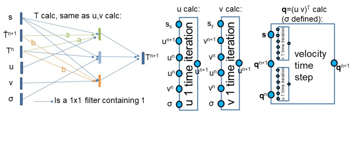
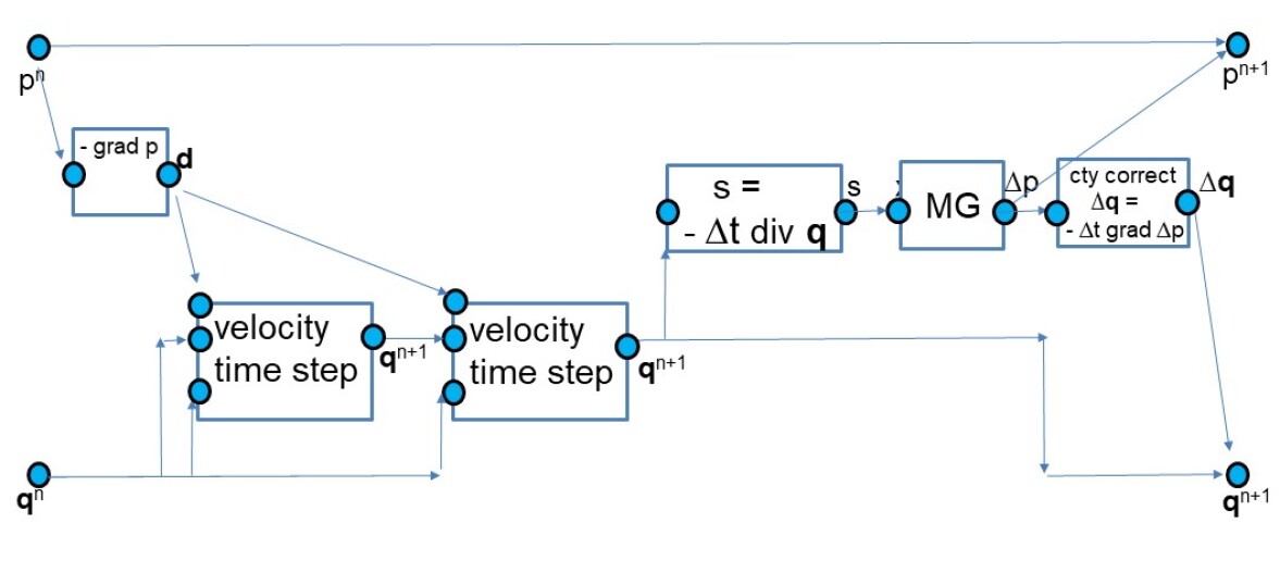
Figure 2: Schematic showing the how the neural networks works for time stepping. Top: For a scalar $T$ and velocity components. The green, orange and purple coloured filters are associated with advection in $u$ and $v$ directions and diffusivity respectively. Bottom: A single time step for the Navier-Stokes solution.

3 Results

In this section we present results for a one-step multigrid solver applied to the advection-diffusion equation; an explicit time discretisation of the advection-diffusion equation; a solution of the nonlinear Burgers equation and finally results are presented for incompressible flow past a bluff body by solving the Navier-Stokes equations combining the methods used in solving the three previous problems. Throughout this section, lengths are in metres, times are in seconds and velocities are in metres per second.

3.1 Multigrid solver for the advection-diffusion equation

Here we show results for the solution of the advection-diffusion equation:

$$\frac{\partial T}{\partial t}+\bm{q}\cdot\nabla T-\nu\nabla\cdot\nabla T=s$$ (27)

by a multigrid method implemented using a CNN. In Equation (27), $T$ is the scalar solution field, $\bm{q}=(1,\;1)^{T}$ is the advection velocity, $s$ the source strength and $\nu$ the constant diffusivity. For a domain measuring 128 by 128, we advect an initial condition of Gaussian distribution centred at $(x_{0},y_{0})=(0,0)$ and the coefficient representing the width of the distribution is $\gamma=10$ (see Equation (28)). The velocity field is uniform at $(u,v)=(1,1)$ and the uniform diffusion coefficient is $k=$2\text{\,}\mathrm{m}^{2}\mathrm{s}^{-1}$$. The finite difference cell sizes in the $x$ and $y$ directions are constant at $\Delta x=\Delta y=1$. The Courant number associated with the grid is $C=50$ and the time step size is $\Delta t=50$. We investigate one time-step solution, starting with an initial guess of $T^{1,0}=T^{0}=0$, using the multigrid with upwind differencing in space for advection and central differencing for diffusion, see Section 2.2. The Jacobi iterative method is embedded in the proposed neural network representing the multigrid method and a skip connection (or skip layer) is used to transfer the residuals between the convolutional layers, see Section 2.1. The numerical methods used to generate these results are implemented by initialising the weights of the kernel of a convolutional layer. No training of the network is performed. The results of applying this network to the initial condition are shown in Figure 3 and indicate the converged numerical prediction by CNN-based multigrid framework. In this figure we show how the solution converges with iteration number. We also show the difference iterations which shows how the multi-grid corrects the solution to obtain the final converged solution. We also show this in graph form and show the residuals at different multi-grid levels which shows how the solution is corrected on each grid level. This shows that the course grids levels seem to do much of the work in representing the solution correction.

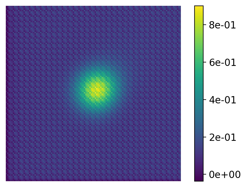
Initial condition, $T^{0}$

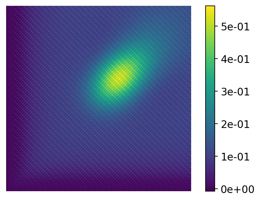
$T^{1,5}$

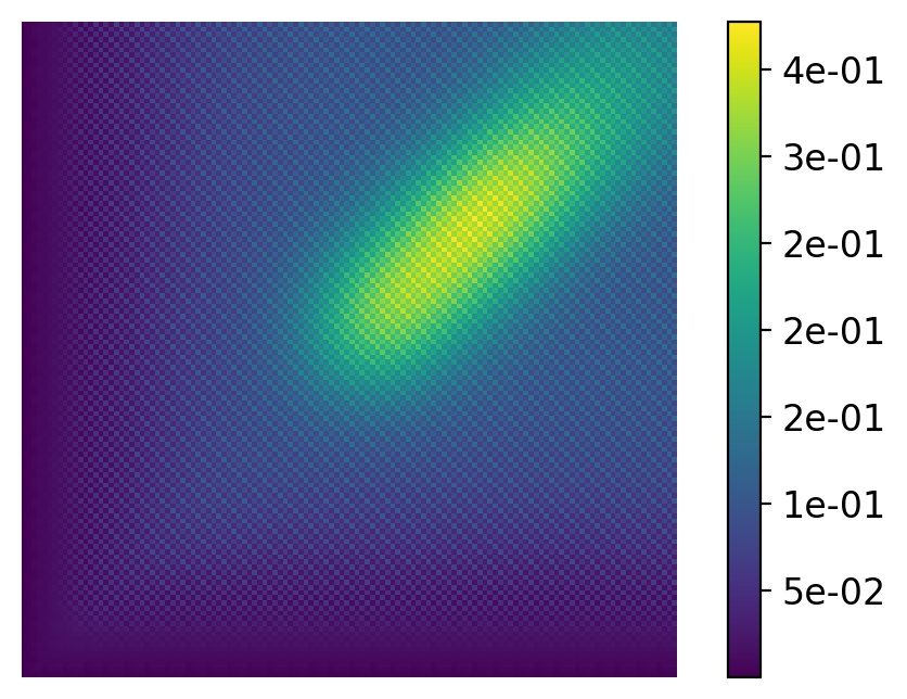
$T^{1,10}$

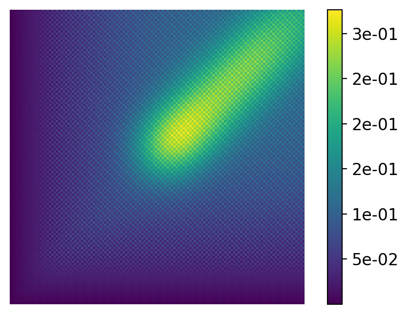
$T^{1,15}$

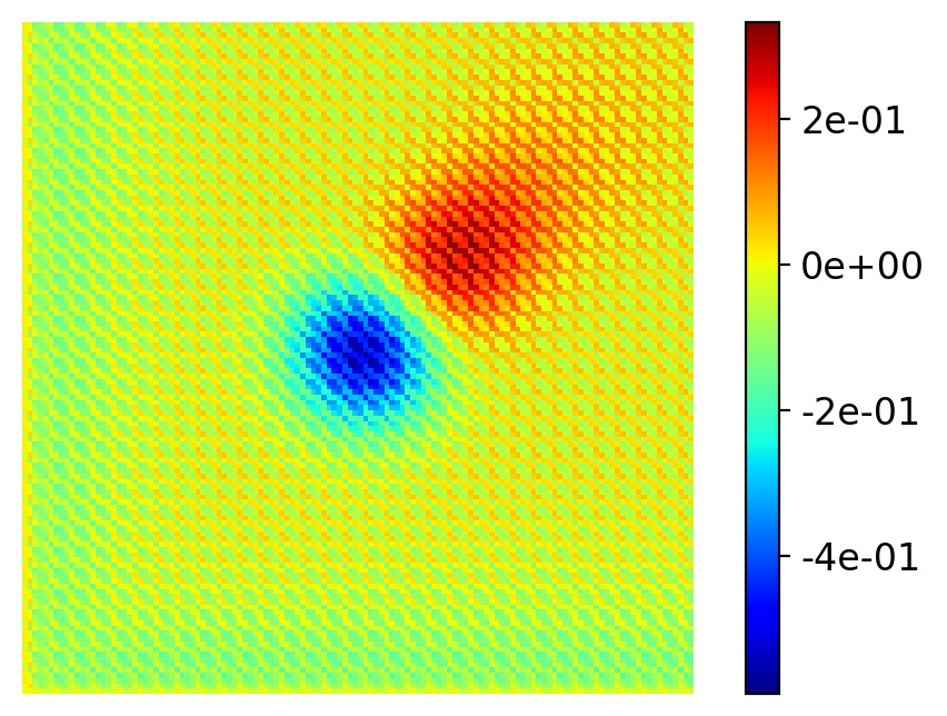
$T^{1,5}-T^{1,0}$

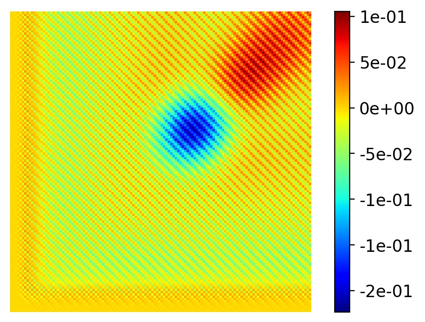
$T^{1,10}-T^{1,5}$

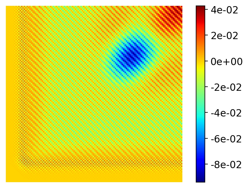
$T^{1,15}-T^{1,10}$

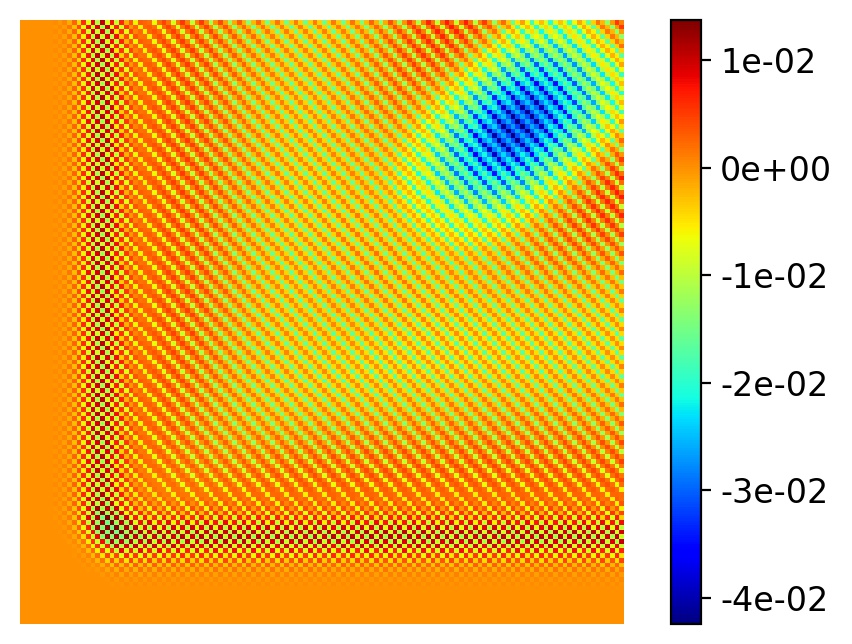
$T^{1,20}-T^{1,15}$

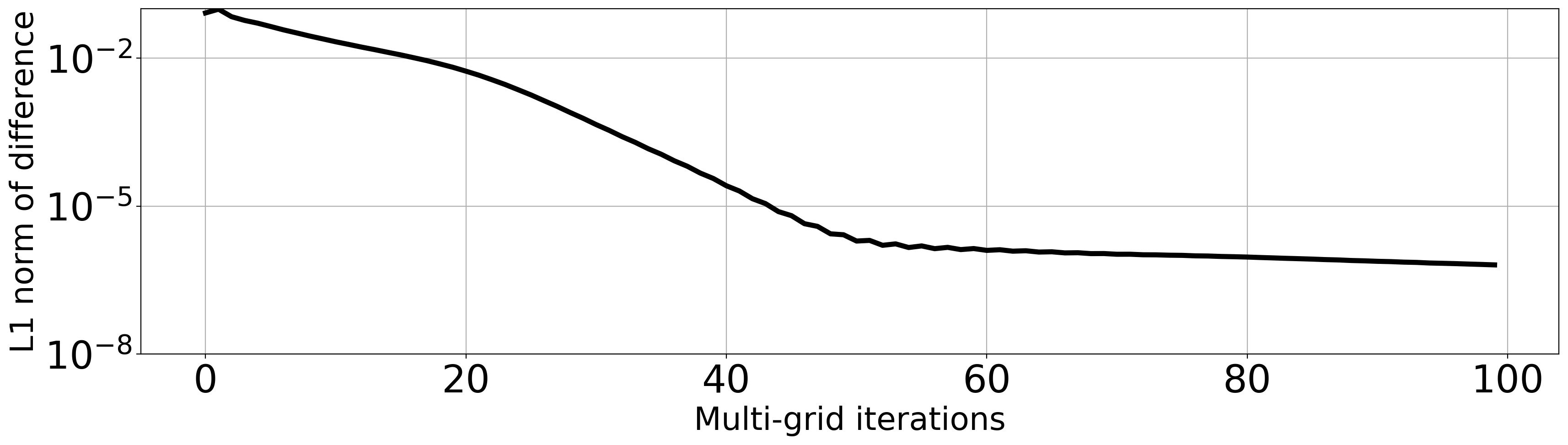
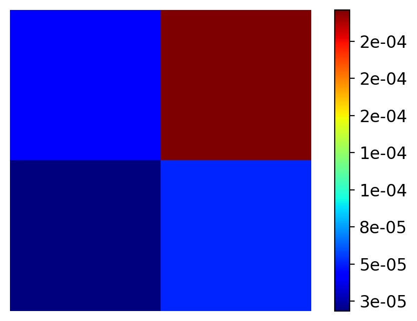
Residual on $2\times 2$

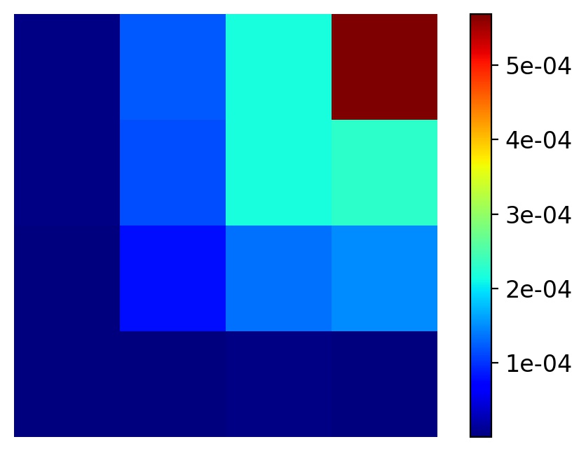
Residual on $4\times 4$

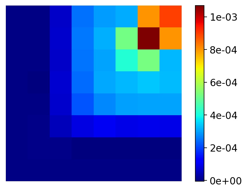
Residual on $8\times 8$

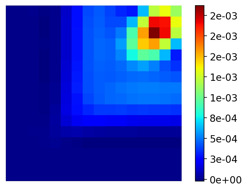
Residual on $16\times 16$

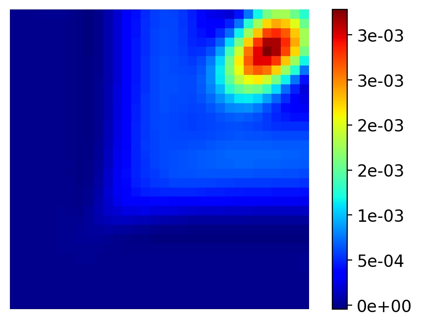
Residual on $32\times 32$

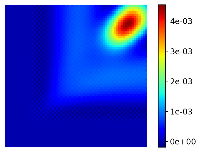
Residual on $64\times 64$

Residual on $128\times 128$

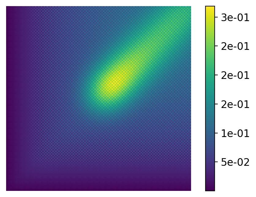
Smoothed solution

Figure 3: Multigrid solution of advection-diffusion equation by a CNN. The first row, at the top, shows the solution with an initial condition of a Gaussian distribution centred at $(x_{0},y_{0})=(0,0)$ after 5, 10 and 15 multigrid iterations ($T^{1,i}$ where $i$ represents the iteration number). The second row shows the difference between the solutions after two particular numbers of iterations. The middle line plot represents the $L_{1}$ norm of difference between the solutions at the current and previous iterations. The last of the bottom 8 plots represents the final solution, and the remaining plots represent the spatial evolution of residuals on different grids within one multigrid iteration.

3.2 Advection-diffusion equation

We apply the proposed CNN to solve the 2D time-dependent advection-diffusion equation in a domain measuring 300 by 300 with the origin located at the centre of the domain. A Gaussian distribution centred in the middle of the domain at $(x_{0},y_{0})=(0,0)$ and with a width of $\gamma=10$ (see Equation (28)) is taken as the initial condition. The advection velocity is $(u,v)=(0,0)$ and the diffusion coefficient $k$ has value $2\text{\,}\mathrm{m}^{2}\mathrm{s}^{-1}$. The model is compared with a traditional PDE solver and tested on different grids, showing that the results are identical to within round-off error (see the line plots in Figure 4). For the same domain, we advect an initial condition with a uniform velocity field $(u,v)=(1,1)$ and a uniform diffusion coefficient $k=$2\text{\,}\mathrm{m}^{2}\mathrm{s}^{-1}$$. The finite difference cell sizes in the $x$ and $y$ directions are constant at $\Delta x=\Delta y=1$. The grid Courant number $C=0.1$ and the time-step size is $\Delta t=0.1$. We investigate the advection and diffusion of a combination of a Gaussian distribution and a square. This combination can be written as

$$T^{0}(x,y) =\exp\left(-\left(\frac{(x-x_{0})^{2}}{2\gamma^{2}}+\frac{(y-y_{0})^{2}}{2\gamma^{2}}\right)\right)$$ (Gaussian distribution) (28)

$$\quad+\begin{cases}1,&\quad x\in\text{[-25,25]},\;y\in\text{[-75,-125]}\\ 0,&\quad\text{otherwise}\end{cases}$$ (Uniform distribution) (29)

in which $T^{0}$ represents the initial condition of the scalar field $T$, $x,y\in[-150,\,150]$, the centre of the Gaussian distribution is at $(x_{0},y_{0})=(-50,0)$, and the coefficient representing the width of the distribution is $\gamma=40$. The square distribution is centred at $(x_{0},y_{0})=(0,-100)$. We investigate two discretisation methods, both with a predictor-corrector time discretisation that is second order accurate and with Crank-Nicolson time stepping: (i) a first order upwind differencing for advection and central differencing for diffusion; (ii) a second order central differencing for both advection and diffusion operators. Both discretisation methods are implemented by specifying the weights of the kernel of a convolutional layer, see Section 2.2 (and by not performing any training). From Figure 4, we see that both methods produce similar results, and, for longer times, the effect of diffusion becomes more pronounced as expected.

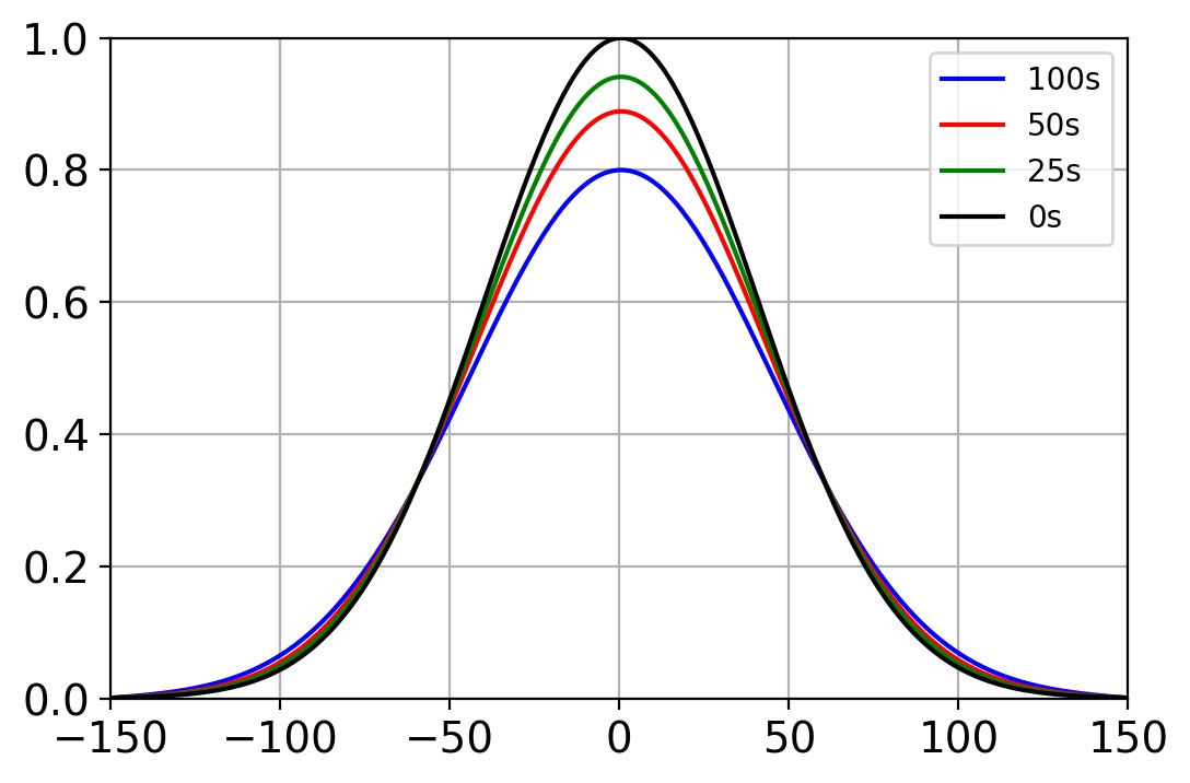
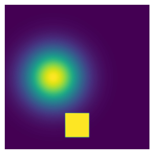
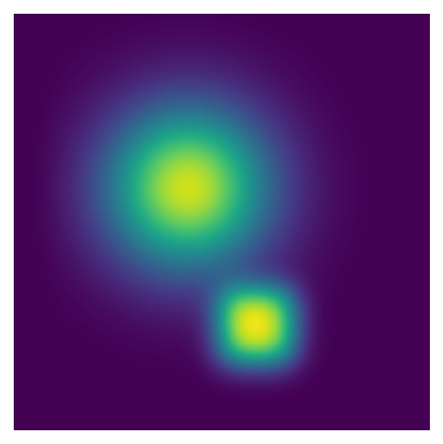
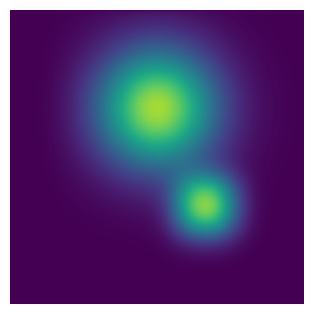
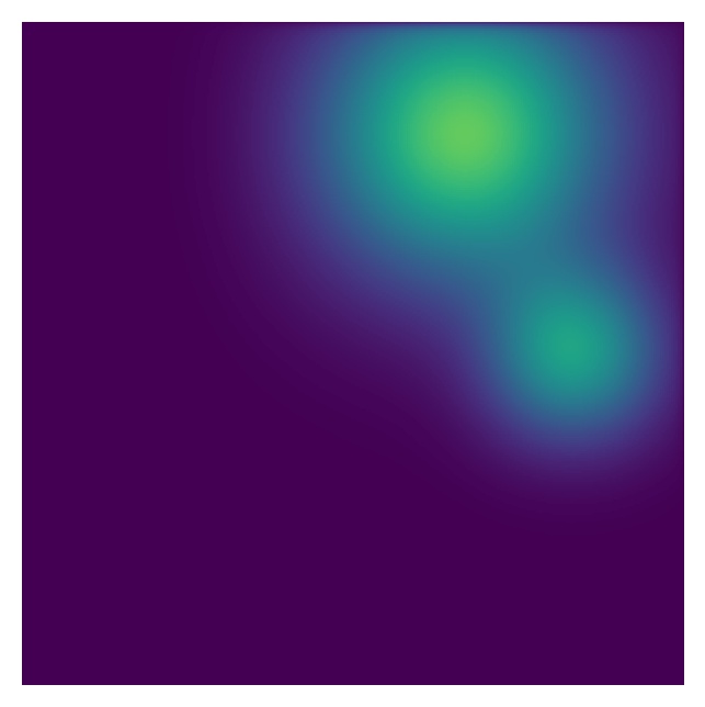
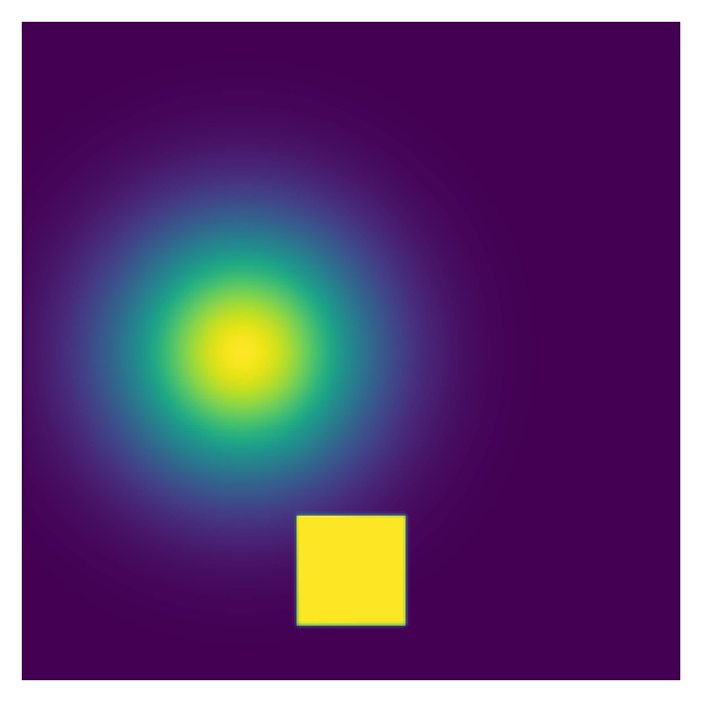
$0\text{\,}\mathrm{s}$

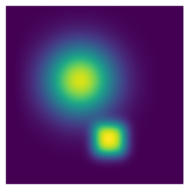
$25\text{\,}\mathrm{s}$

$50\text{\,}\mathrm{s}$

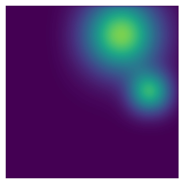
$100\text{\,}\mathrm{s}$

Figure 4: Numerical solution of the advection-diffusion equation by a CNN at 0, 25, 50 and 100. The top two line plots compare the solution of the advection-diffusion equation (with no advection) for an initial condition of a Gaussian distribution by a traditional fluid dynamics code (left) and using the approach described here based on CNNs (right). The three values shown in each graph correspond to the maximum values of the solution, occurring at $x$=0. The eight contour plots relate to the solution of the advection-diffusion equation for an initial condition of the combination of a square and a Gaussian centred at $(x_{0},y_{0})=(0,-100)$ and $(x_{0},y_{0})=(-50,0)$ respectively. Both sets of results have a second-order time discretisation scheme with central differencing in space for the diffusion operator. The plots on row (a) have upwind differencing for the advection operator; and on row (b) have central differencing for the advection operator.

3.3 Burgers equation

For a domain measuring 300 by 300 with the origin at the centre of this, we validate the CNN which has been initialised in such a way that it can solve the Burgers equation on different grids and compare the results with a PDE solver. The results from the CNN and the traditional PDE solver were found to be identical up to round-off errors. Subsequently, two tests were performed. The first with a $v$ velocity component of zero (which remains at zero throughout) and a $u$ velocity component that is initialised using the Gaussian distribution, (see the first term in Equation (28)). The finite difference cell sizes in the increasing $x$ and $y$ directions are constant at $\Delta x=\Delta y=1$. For the first example, the Gaussian distribution is centred at $(x_{0},y_{0})=(-100,0)$ with a width defined by $\gamma=15$. For the second example, the Gaussian (associated with $u^{0}(x,y)$ and $v^{0}(x,y)$) is centred at $(x_{0},y_{0})=(0,0)$ with a width of $\gamma=$40\text{\,}\mathrm{m}$$. In these examples, the viscosity, absorption and source terms of the Burgers equation are set to zero. We run both simulations with central differencing in space for diffusion and a predictor-corrector time discretisation scheme. First-order upwind differencing and central differencing schemes in space are used for the advection. The Courant number is set to be $C=0.1$ using $\Delta t=0.1$. To solve the Burgers equation, the discretisation schemes are coded as proposed, by initialising the weights of the kernel of a convolutional layer, but also by modifying the activation function so it is able to capture the non-linearity of the Burgers equation, see Section 2.3. The results can be seen in Figure 5. We see that the method resolves the non-linearity of Burgers equation resulting in the expected shock formation.

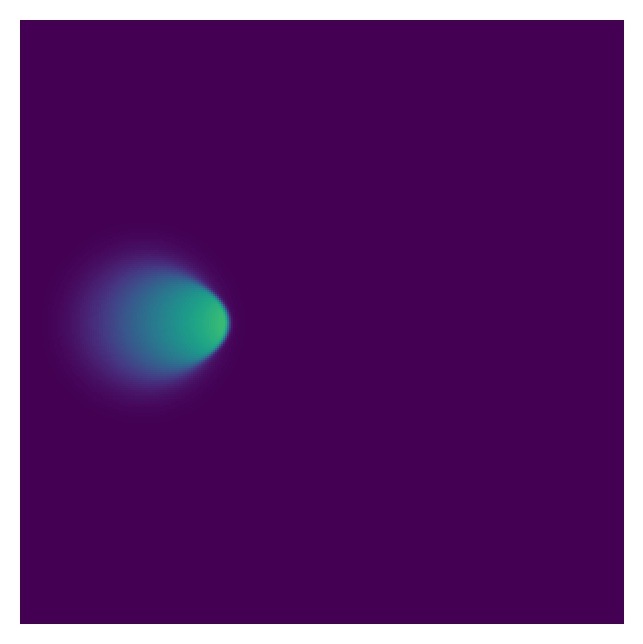
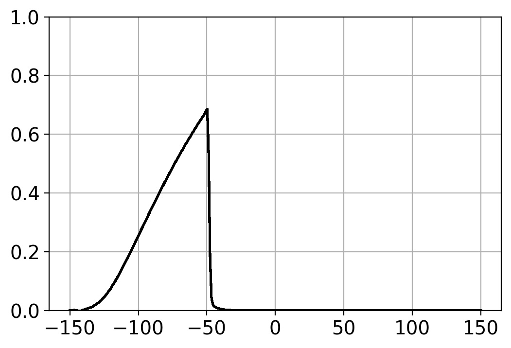
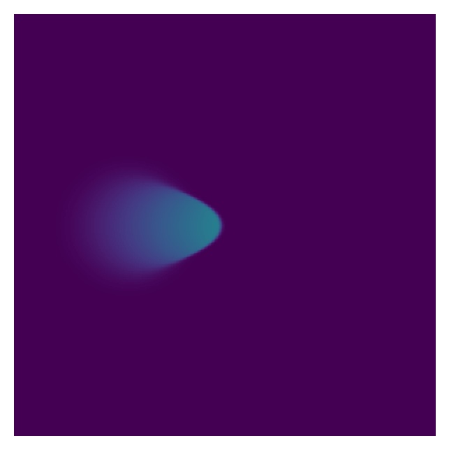
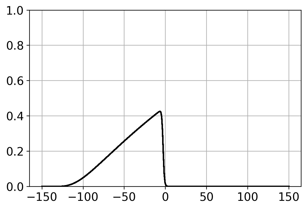
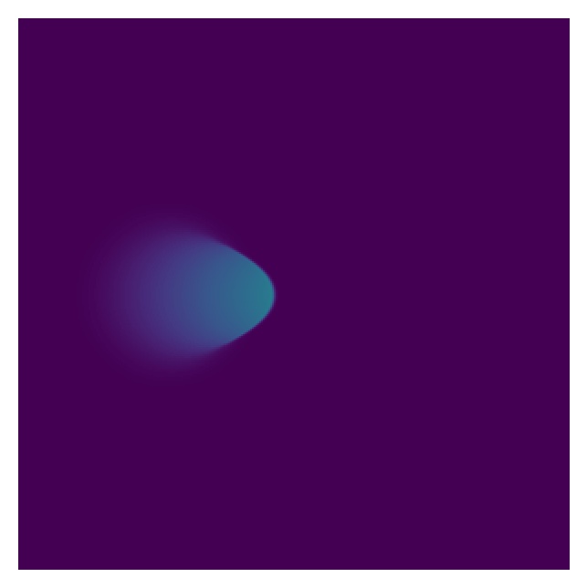
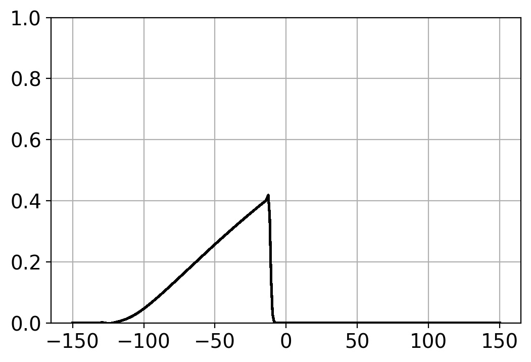
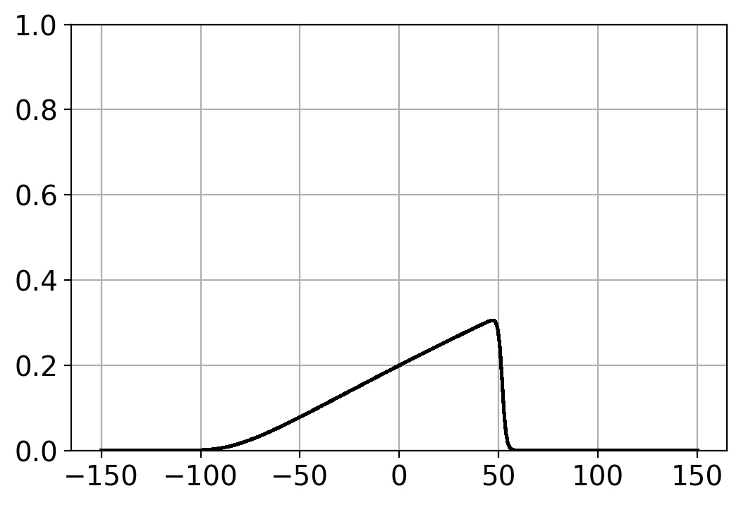
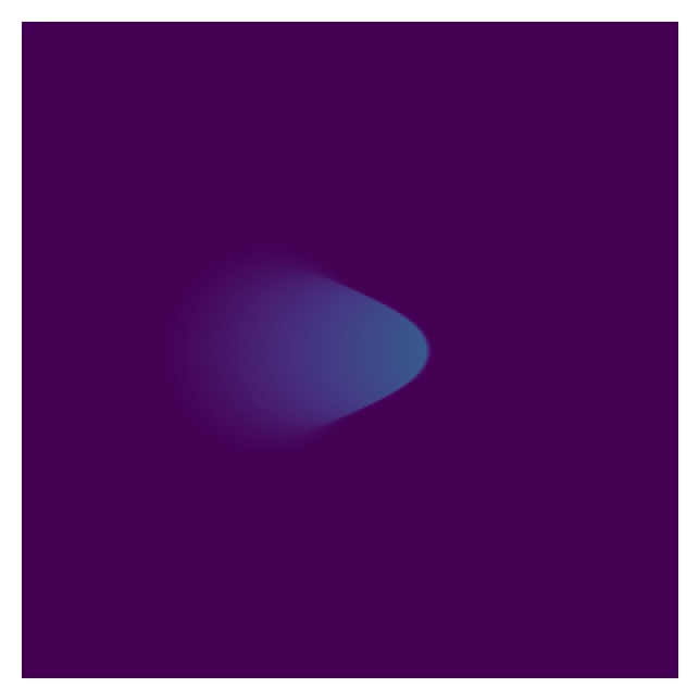
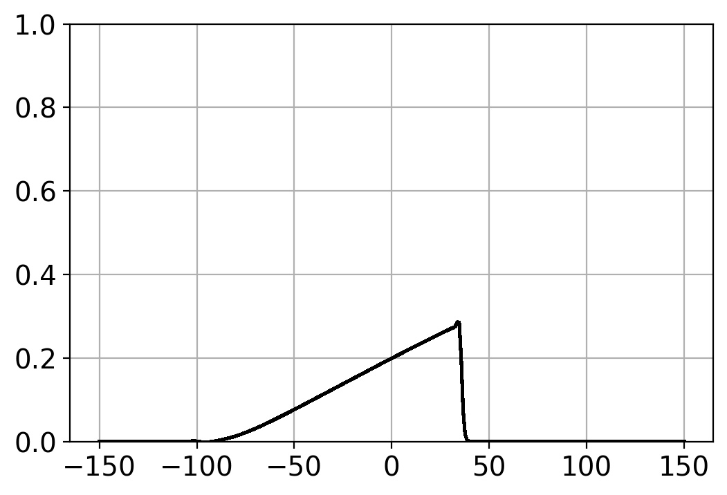
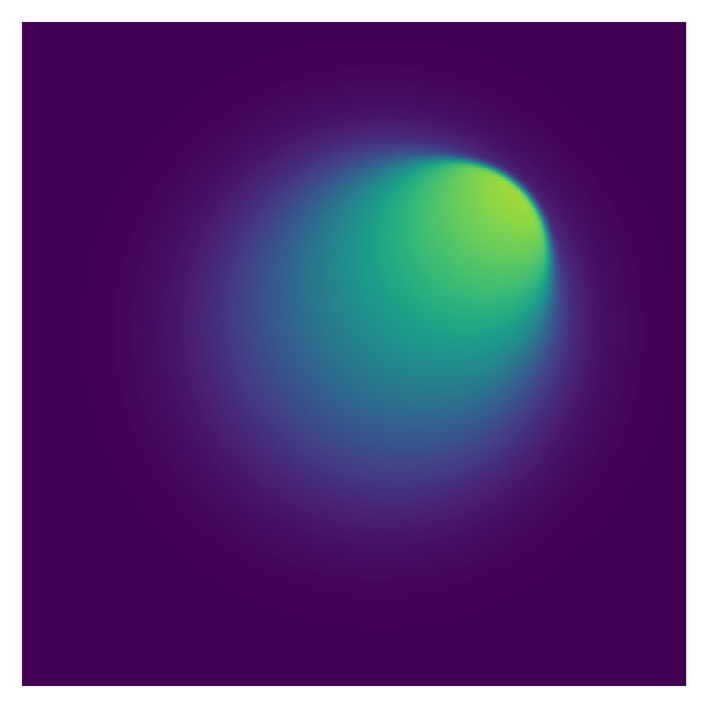
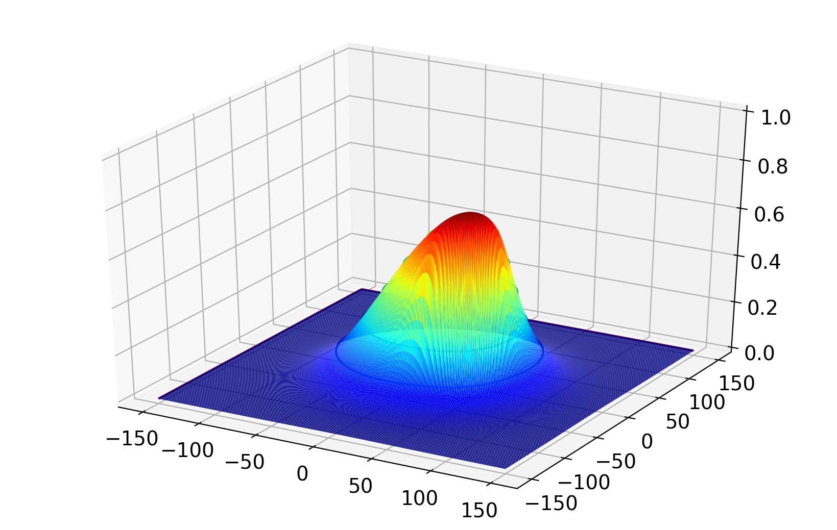
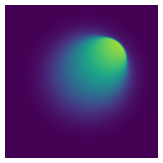
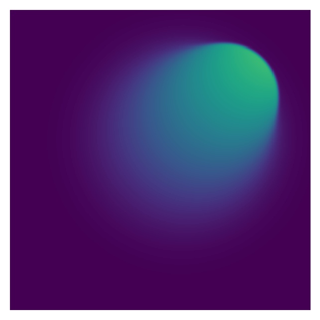
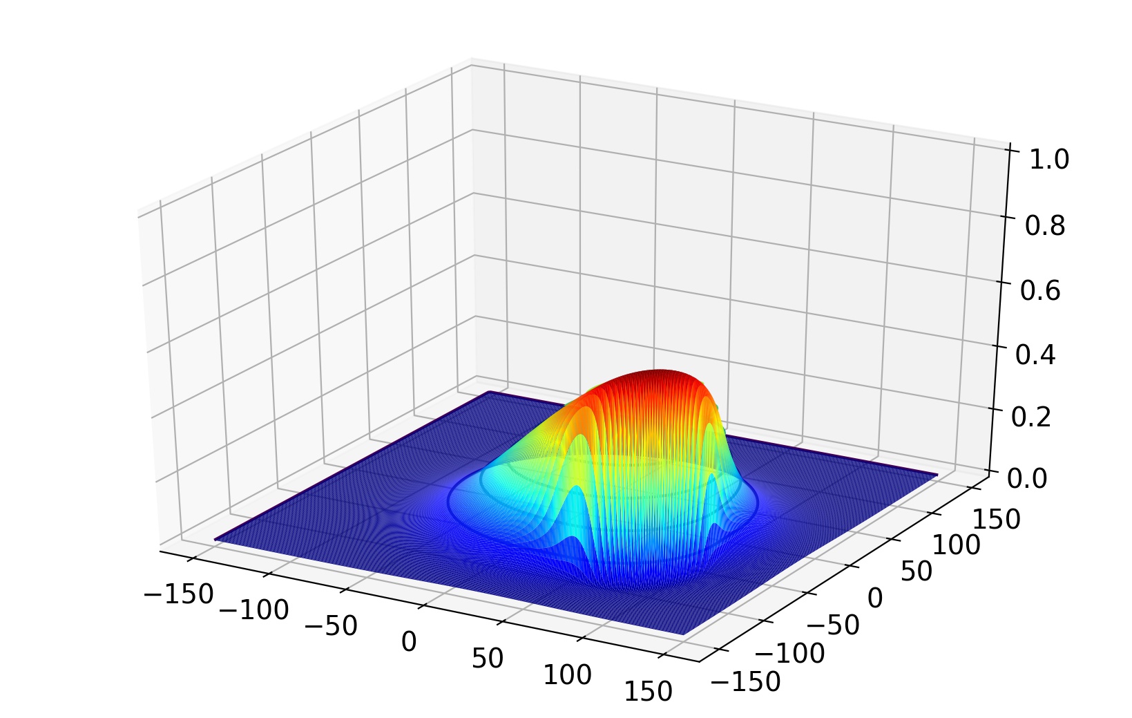
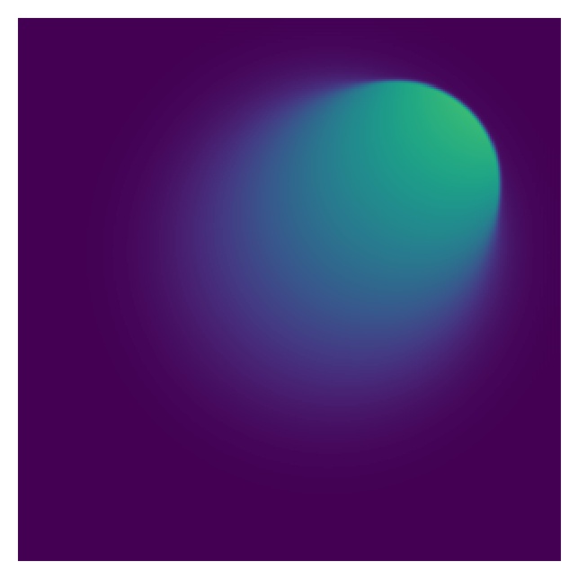
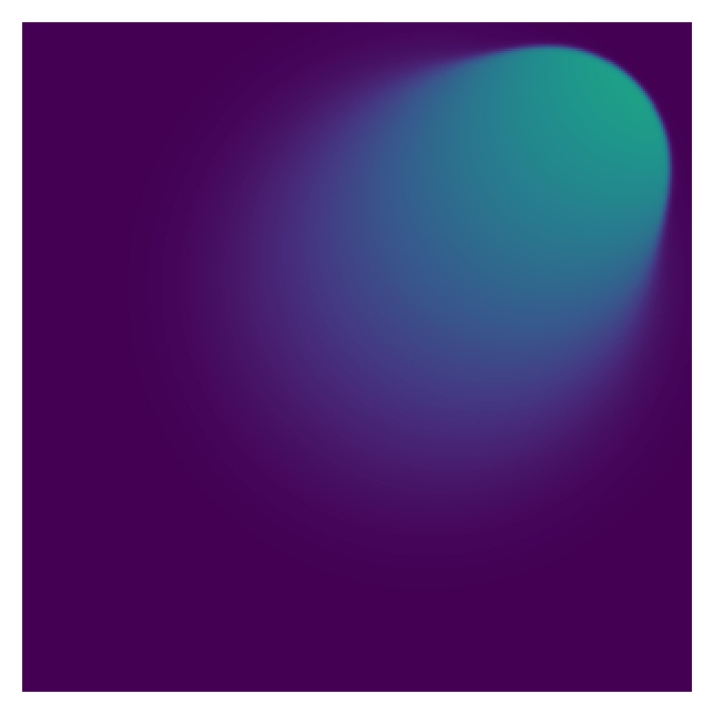
(a)

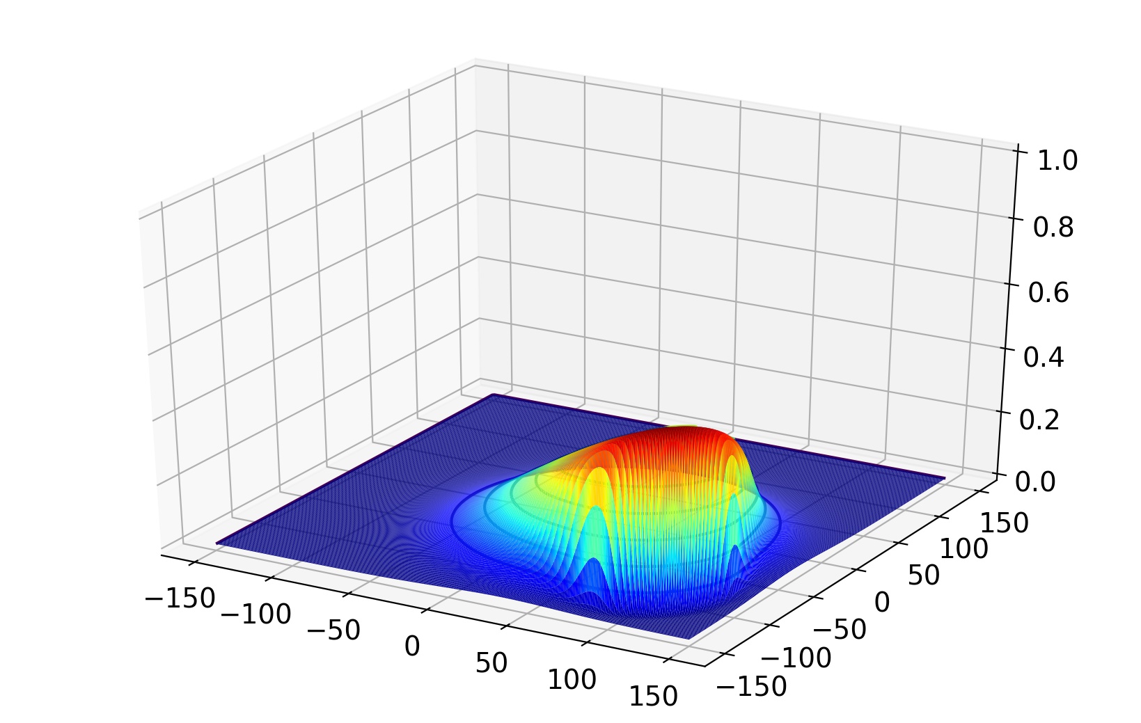
(b)

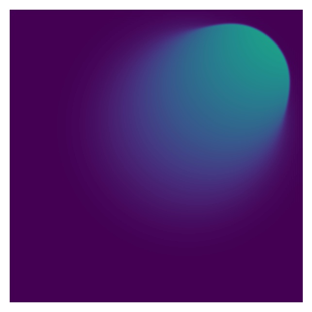
(c)

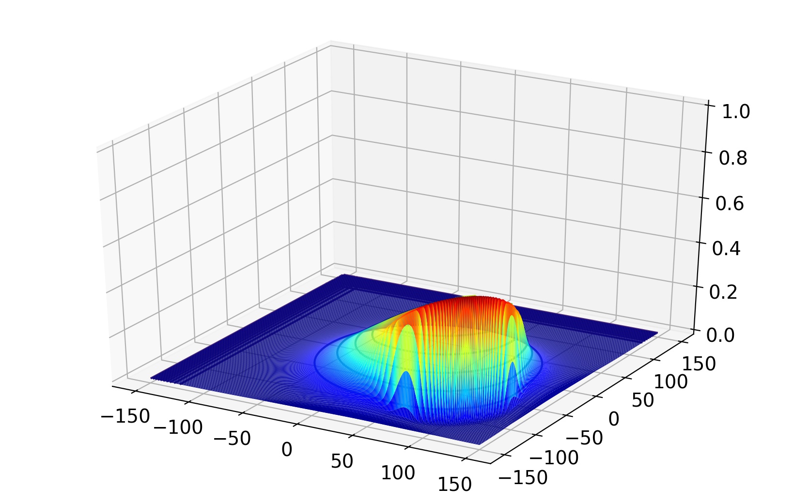
(d)

Figure 5: Numerical prediction of 2D nonlinear Burgers equation by a CNN. The top 12 plots relate to the flow field with only the $u$ component and a Gaussian-shaped wave initially centred at $(x_{0},y_{0})=(-100,0)$, at 10, 30 and 60. The bottom 12 plots relate to the flow field with the $u$ and $v$ components and a Gaussian-shaped wave initially centred at $(x_{0},y_{0})=(0,0)$, at 10, 30 and 60. Columns represent second-order time stepping scheme: (a) and (b) upwind differencing for advection operator and central differencing for diffusion operator in space; (c) and (d) upwind differencing for advection operator and second-order central differencing for diffsuion operator in space.

3.4 Flow past a bluff body with Navier-Stokes equations

Here we integrate the proposed ability of the CNN to forecast 2D and 3D flow past a bluff body by solving the incompressible Navier-Stokes equations as described in Section 2.4. The domain has dimensions 512 by 512 and has a 40 by 40 solid square block centred at $(x_{0},y_{0})=(128,256)$. The cell size is uniform in the $x$ and the $y$ directions ($\Delta x$ and $\Delta y$) and set to 1. The initial velocity and pressure fields are set to zero across the whole domain. A zero pressure boundary condition is imposed at the right boundary and other three sides are applied with zero derivative boundary condition for the pressure field. Boundary conditions for the velocity field include the use of the slip boundary condition at the bottom and the top walls. An inflow and an outflow velocity in the $x$-direction of 1 are imposed at the left and the right boundaries and a velocity in the $y$-direction of 0 is imposed on these boundaries. The Reynolds number used here is $200$ and is specified through the viscosity of the flow, assuming a unity density. We run the simulation with central differencing in space for the viscous and advection terms, while a second order accurate predictor-corrector scheme is applied to discretise the time derivative, see Section 2.2. A fixed time step $\Delta=0.1$ is used. To solve the Navier-Stokes equations, the discretisation scheme is coded by initialising the weights of the kernel of a convolutional layer. The two components of the velocity field $u,v$ for 2D and three velocity components $u,v,w$, in 3D, are treated separately as inputs of the neural network. The pressure field is obtained by applying multigrid networks to solve the resulting Poisson equation, see Equation (25). The activation function is modified to capture the non-linearity of the advection terms. The results are shown in Figure 6. We see that the method resolves the flow structures around bluff body, including the unsteady separation of flow and vortex shedding. In the 2D AI simulation, the non-dimensional frequency of vortex shedding or Strouhal number is calculated to be $0.142$ from our results for $Re=200$, which is very close to the database value of 0.147 established by [33]. We further explore the vortex structure in 3D flow past a bluff body by extending the proposed network into 3D. For this case, the dimension of the domain is 128 by 128 by 128 with a 10 by 10 by 10 solid square block centred at $(x_{0},y_{0},z_{0})=(32,64,64)$ and in which the solution domain is defined by $x\in[0,128],\;y\in[0,128],z\in[0,128]$. The results are shown in Figure 6(a)-(c). The length of the re-circulation bubble $l_{1}$ is $22\text{\,}\mathrm{m}$ and the distance between the centre of the circulation bubble where there is no velocity and the cube $l_{2}$ is $10\text{\,}\mathrm{m}$. The ratio of $l_{1}$ to $l_{2}$ can be computed as 2.2, showing a close agreement with the value calculated in [34]. The AI solver’s computational efficiency is assessed on various computing architectures, with the Intel Xeon 2.3Ghz CPU and NVIDIA Tesla T4 GPU (featuring 2560 CUDA cores) being chosen. The study involves testing three 3D cases comprising $128^{3}$, $256^{3}$ and $512^{3}$ finite element nodes, each running for five time steps with 20 multigrid iterations per time step. The results reveal that for the $128^{3}$ case, a single CPU requires 165 seconds, while a single GPU completes the task in 3 seconds. Similarly, for the $256^{3}$ case, a single CPU requires 1275 seconds, while a single GPU takes only 11 seconds. Finally, for the $512^{3}$ case, a single CPU requires 14,376 seconds, while a single GPU completes the task in 34 seconds.

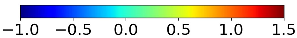
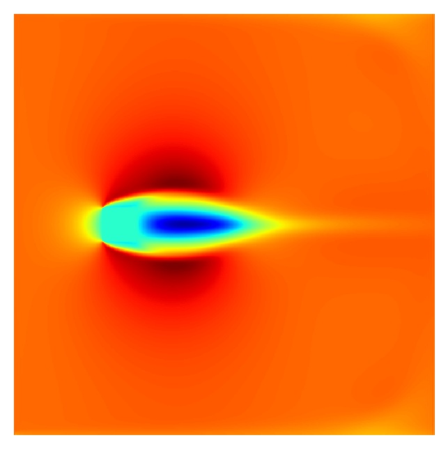
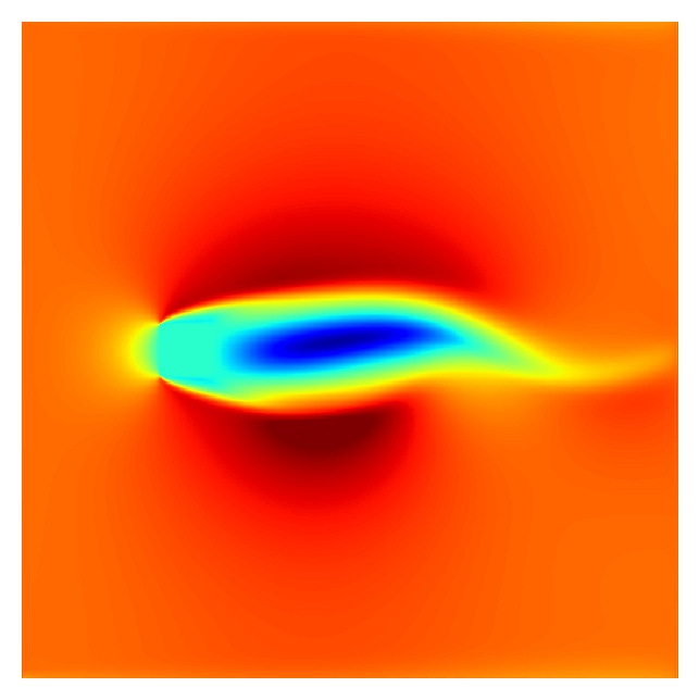
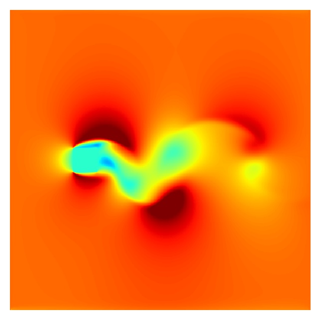
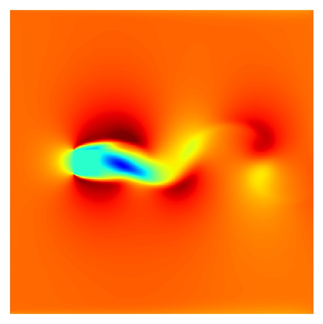
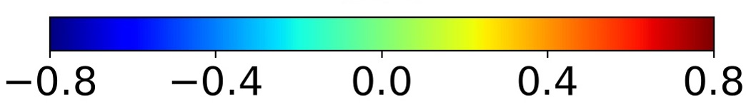
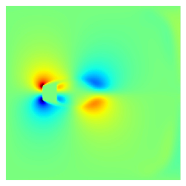
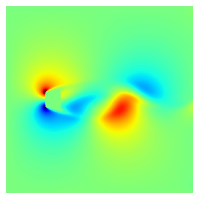
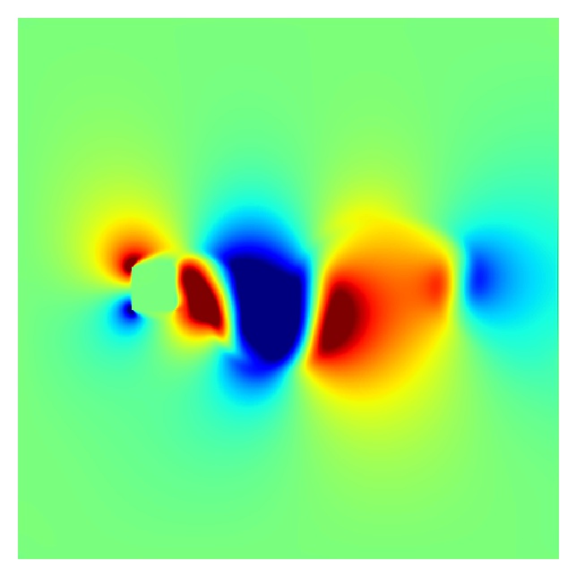
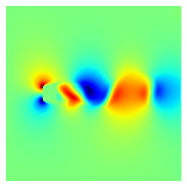
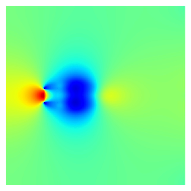
500s

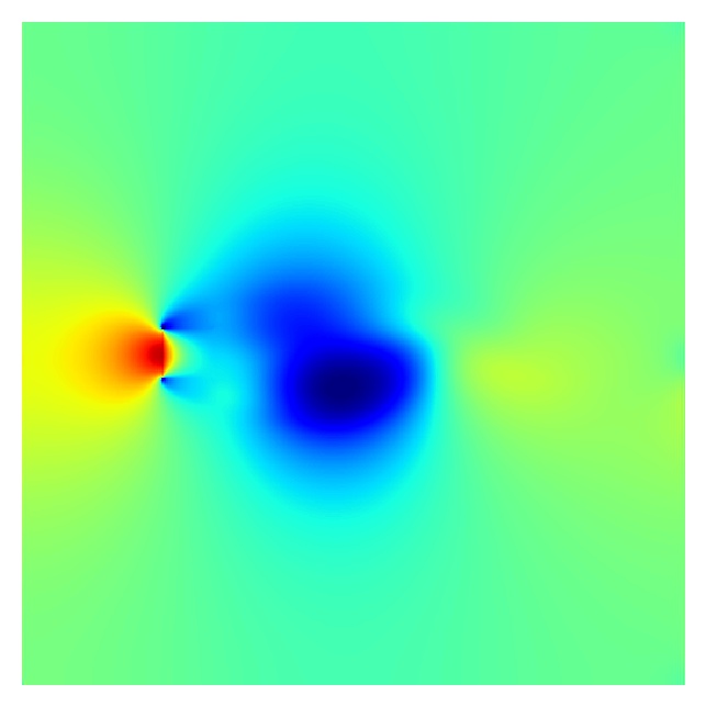
1000s

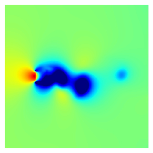
1500s

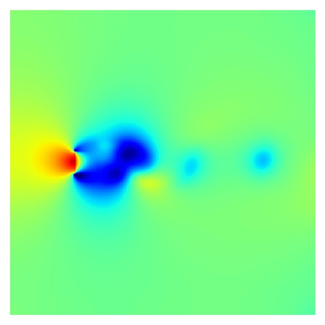
2000s

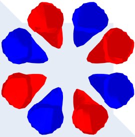
(a)

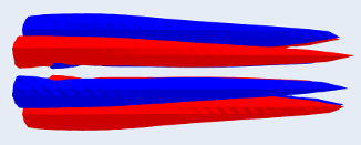
(b)

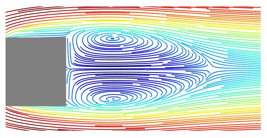
(c)

Figure 6: Numerical prediction of 2D and 3D flow past a bluff body by a CNN. The 12 plots relate to the two velocities and the pressure of the 2D flow field, at $500\text{\,}\mathrm{s}$, $1000\text{\,}\mathrm{s}$, $1500\text{\,}\mathrm{s}$ and $2000\text{\,}\mathrm{s}$. The dimension of 2D computational domain is $512\text{\,}\mathrm{m}$ by $512\text{\,}\mathrm{m}$, where a solid square body is modelled as $40\text{\,}\mathrm{m}$ by $40\text{\,}\mathrm{m}$ and centred at $(x_{0},y_{0})=($128\text{\,}\mathrm{m}$,$256\text{\,}\mathrm{m}$)$. The bottom 3 plots relate to the steady vortex structure in the 3D flow field at $1000\text{\,}\mathrm{s}$: (a) and (b) are the rear and side views of the isosurface representing $\omega_{x}=\pm 0.01$ with red and blue for positive and negative; (c) is 2D steady streamlines coloured by the u-component velocity. The dimension of 3D computational domain is $128\text{\,}\mathrm{m}$ by $128\text{\,}\mathrm{m}$ by $128\text{\,}\mathrm{m}$, where a solid square body is modelled as $10\text{\,}\mathrm{m}$ by $10\text{\,}\mathrm{m}$ by $10\text{\,}\mathrm{m}$ and centred at $(x_{0},y_{0},z_{0})=($32\text{\,}\mathrm{m}$,$64\text{\,}\mathrm{m}$,$64\text{\,}\mathrm{m}$)$. The Reynolds number of the two case is set by 200. Both sets of results have a second-order time discretisation scheme with central differencing in space for the diffusion and the advection.

4 Discussion and Conclusion

We have demonstrated how neural networks can be used to solve differential equations, and have presented some simple applications and theory to underpin the approach. Implementing discretisations of PDEs using AI libraries with the method proposed here, has been found to produce identical results, to within round-off error, to PDE solvers written in more conventional programming languages e.g. modern Fortran. This, and similar work that is underway, is showing how the vast quantity of highly optimised AI software can be leveraged to solve differential equations across disciplines. For example, in fluids, solids, electromagnetism, radiation, economics or finance.

Programming PDE solutions using AI software is potentially very important because it enables interoperability between GPUs, CPUs and AI computers, which, in turn, enables exploitation of AI community software. Furthermore, energy shortfalls and climate change mean that the use of energy efficient computers will become increasingly desirable. Running software on any new architecture can be difficult, however, as these machines are designed to run AI software, this problem will have already been solved. Finally, it is also important because it can help to combine AI-based Reduced-Order Modelling (referred to here as AI-Physics modelling) and discretisation of the differential equations, facilitating a number of approaches including AI-based Subgrid-Scale (SGS) models and physics-informed methods [35]. It is now accepted that future SGS methods will be increasingly based on AI and that these often require implicit coupling to CFD: AI programming is the only satisfactory implementation approach.

The key advantages of programming numerical discretisations of PDEs using AI software include: (a) relatively easy implementation of multigrid methods and preconditioners; (b) model hierarchies can be readily formed ranging from high fidelity CFD to both fine and coarse AI-Physics models to make the methods much more computationally efficient; (c) CFD and AI-Physics modelling can be embedded in a single neural network, which is necessary for the implicit treatment within CFD of sophisticated SGS models based on AI and Physics-Informed methods; (d) automatic adjoint generation for digital twins that are able to assimilate data, perform uncertainty quantification and optimisation (see [36, 37]) using the optimisation engines embedded in all AI software, see [36]; (e) the realisation of new features in modelling without writing large quantities of code (e.g. mixed arithmetic precision or coupling different physics); (f) using AI software would make model development more accessible than programming within existing CFD codes, which can be highly complex; (g) the code generated by programming in AI software would be automatically optimised and be interoperable between computer architectures: CPU, GPU and AI computers, including exascale computers; (h) long term sustainability as code is based on long standing, community supported, AI software. For unstructured meshes and parallel computing one can generalise the above approach. For example, model parallelisation can be implemented, using MPI message passing to update the halos on the perimeters of the partitioned subdomains. In addition, this approach also allows blocks of different patterns to be used which enables semi-structured or block structured grids to be used and merges the use of parallelisation and unstructured meshes: more than one subdomain can be used on a given core using the MPI approach. In addition, the stencils or discretisations associated with fully unstructured meshes can be held on graph neural networks (see [38, 39]) in which there is no structured stencil. Instead, there is a sparse graph just as with an unstructured finite element method. On this graph we can define the discretisations as we have done before, except there may be a need to define every weight individually associated with the edges of the graph rather than using convolutional filters.

To form the multigrid method we can take the approach of coarsening the graph as often done in graph CNNs, see [40]. However, one can use mappings to structured 1D grids as used in the Space Filling Curve (SFC) CNN approach, see [41]. This is particularly efficient as the 1D grid structure can map highly efficiently onto the memory of the computer and with no indirect addressing.

For unstructured meshes, one can generalise the above approach by using graph neural networks (GNNs) [38, 39]. When using multigrid methods, the graph can be coarsened, as often done in GNN approaches [40] or one could use space-filling curves to generate mapping to structured 1D grids [41]. The latter could be highly efficacious as the 1D grid structure can map efficiently onto the memory of the computer, with no indirect addressing. To implement the parallelism, message passing (MPI) can be used to update the halos on the perimeters of the partitioned subdomains. We intend to explore these possibilities in the future.

Appendix A Filters

2D and 3D Convolutional Filters for Diffusion and Advection Discretization

The 3 by 3 filters implemented in the proposed 2D and 3D convolutional neural networks are shown below based on $\Delta t=0.1s$, $\Delta x=1\;\text{m}$ and $u=1\;\text{m}\text{s}^{-1}$. 2D 5-point stencil (diffusion operator, advection operator in $x$ and advection operator in $y$ in which $u$ and $v$ are the advection velocity components in the increasing $x-$ and $y-$directions)

$$\nu\frac{\Delta t}{\Delta x^{2}}\left(\begin{array}[]{rrr}0.0&1.0&0.0\\ 1.0&-4.0&1.0\\ 0.0&1.0&0.0\\ \end{array}\right),\frac{\Delta t\,u}{\Delta x}\left(\begin{array}[]{rrr}0.0&0.0&0.0\\ 0.5&0.0&-0.5\\ 0.0&0.0&0.0\\ \end{array}\right),\frac{\Delta t\,v}{\Delta x}\left(\begin{array}[]{rrr}0.0&-0.5&0.0\\ 0.0&0.0&0.0\\ 0.0&0.5&0.0\\ \end{array}\right).$$

2D 9-point stencil (diffusion operator, advection operator in $x$ and advection operator in $y$)

$$\nu\frac{\Delta t}{\Delta x^{2}}\left(\begin{array}[]{rrr}0.25&0.5&0.25\\ 0.5&-3.0&0.5\\ 0.25&0.5&0.25\\ \end{array}\right),\frac{\Delta t\,u}{\Delta x}\left(\begin{array}[]{rrr}0.08&0.0&-0.08\\ 0.33&0.0&-0.33\\ 0.08&0.0&-0.08\\ \end{array}\right),\frac{\Delta t\,v}{\Delta x}\left(\begin{array}[]{rrr}-0.08&-0.33&-0.08\\ 0.0&0.0&0.0\\ 0.08&0.33&0.08\\ \end{array}\right).$$

3D 7-point stencil diffusion operator (1st layer, 2nd layer and 3rd layer)

$$\nu\frac{\Delta t}{\Delta x^{2}}\left(\begin{array}[]{rrr}0.0&0.0&0.0\\ 0.0&1.0&0.0\\ 0.0&0.0&0.0\\ \end{array}\right),\nu\frac{\Delta t}{\Delta x^{2}}\left(\begin{array}[]{rrr}0.0&1.0&0.0\\ 1.0&-6.0&1.0\\ 0.0&1.0&0.0\\ \end{array}\right),\nu\frac{\Delta t}{\Delta x^{2}}\left(\begin{array}[]{rrr}0.0&0.0&0.0\\ 0.0&1.0&0.0\\ 0.0&0.0&0.0\\ \end{array}\right).$$

3D 7-point stencil advection operator in $x$ (1st layer, 2nd layer and 3rd layer)

$$\frac{\Delta t\,u}{\Delta x}\left(\begin{array}[]{rrr}0.0&0.0&0.0\\ 0.0&0.0&0.0\\ 0.0&0.0&0.0\\ \end{array}\right),\frac{\Delta t\,u}{\Delta x}\left(\begin{array}[]{rrr}0.0&0.0&0.0\\ 0.5&0.0&-0.5\\ 0.0&0.0&0.0\\ \end{array}\right),\frac{\Delta t\,u}{\Delta x}\left(\begin{array}[]{rrr}0.0&0.0&0.0\\ 0.0&0.0&0.0\\ 0.0&0.0&0.0\\ \end{array}\right).$$

3D 7-point stencil advection operator in y (1st layer, 2nd layer and 3rd layer)

$$\frac{\Delta t\,v}{\Delta x}\left(\begin{array}[]{rrr}0.0&0.0&0.0\\ 0.0&0.0&0.0\\ 0.0&0.0&0.0\\ \end{array}\right),\frac{\Delta t\,v}{\Delta x}\left(\begin{array}[]{rrr}0.0&-0.5&0.0\\ 0.0&0.0&0.0\\ 0.0&0.5&0.0\\ \end{array}\right),\frac{\Delta t\,v}{\Delta x}\left(\begin{array}[]{rrr}0.0&0.0&0.0\\ 0.0&0.0&0.0\\ 0.0&0.0&0.0\\ \end{array}\right).$$

3D 7-point stencil advection operator in z (1st layer, 2nd layer and 3rd layer, $w$ is the velocity component in the $z-$direction)

$$\frac{\Delta t\,w}{\Delta x}\left(\begin{array}[]{rrr}0.0&0.0&0.0\\ 0.0&0.5&0.0\\ 0.0&0.0&0.0\\ \end{array}\right),\frac{\Delta t\,w}{\Delta x}\left(\begin{array}[]{rrr}0.0&0.0&0.0\\ 0.0&0.0&0.0\\ 0.0&0.0&0.0\\ \end{array}\right),\frac{\Delta t\,w}{\Delta x}\left(\begin{array}[]{rrr}0.0&0.0&0.0\\ 0.0&-0.5&0.0\\ 0.0&0.0&0.0\\ \end{array}\right).$$

3D 27-point stencil diffusion operator (1st layer, 2nd layer and 3rd layer)

$$\nu\frac{\Delta t}{\Delta x^{2}}\left(\begin{array}[]{rrr}0.077&0.115&0.077\\ 0.115&0.231&0.115\\ 0.077&0.115&0.077\\ \end{array}\right),\nu\frac{\Delta t}{\Delta x^{2}}\left(\begin{array}[]{rrr}0.115&0.231&0.115\\ 0.231&-3.385&0.231\\ 0.115&0.231&0.115\\ \end{array}\right),$$

$$\nu\frac{\Delta t}{\Delta x^{2}}\left(\begin{array}[]{rrr}0.077&0.115&0.077\\ 0.115&0.231&0.115\\ 0.077&0.115&0.077\\ \end{array}\right).$$

3D 27-point stencil advection operator in $x$ (1st layer, 2nd layer and 3rd layer)

$$\frac{\Delta t\,u}{\Delta x}\left(\begin{array}[]{rrr}0.014&0.0&-0.014\\ 0.056&0.0&-0.056\\ 0.014&0.0&-0.014\\ \end{array}\right),\frac{\Delta t\,u}{\Delta x}\left(\begin{array}[]{rrr}0.056&0.0&-0.056\\ 0.22&0.0&-0.22\\ 0.056&0.0&-0.056\\ \end{array}\right),\frac{\Delta t\,u}{\Delta x}\left(\begin{array}[]{rrr}0.014&0.0&-0.014\\ 0.056&0.0&-0.056\\ 0.014&0.0&-0.014\\ \end{array}\right).$$

3D 27-point stencil advection operator in $y$ (1st layer, 2nd layer and 3rd layer)

$$\frac{\Delta t\,v}{\Delta x}\left(\begin{array}[]{rrr}-0.014&-0.056&-0.014\\ 0.0&0.0&0.0\\ 0.014&0.056&-0.014\\ \end{array}\right),\frac{\Delta t\,v}{\Delta x}\left(\begin{array}[]{rrr}-0.056&-0.22&-0.056\\ 0.0&0.0&0.0\\ 0.056&0.22&0.056\\ \end{array}\right),$$

$$\frac{\Delta t\,v}{\Delta x}\left(\begin{array}[]{rrr}-0.014&-0.056&-0.014\\ 0.0&0.0&0.0\\ 0.014&0.056&-0.014\\ \end{array}\right).$$

3D 27-point stencil advection operator in $z$ (1st layer, 2nd layer and 3rd layer)

$$\frac{\Delta t\,w}{\Delta x}\left(\begin{array}[]{rrr}0.014&0.056&0.014\\ 0.056&0.22&0.056\\ 0.014&0.056&0.014\\ \end{array}\right),\frac{\Delta t\,w}{\Delta x}\left(\begin{array}[]{rrr}0.0&0.0&0.0\\ 0.0&0.0&0.0\\ 0.0&0.0&0.0\\ \end{array}\right),\frac{\Delta t\,w}{\Delta x}\left(\begin{array}[]{rrr}-0.014&-0.056&-0.014\\ -0.056&-0.22&-0.056\\ -0.014&-0.056&-0.014\\ \end{array}\right).$$

References

- Dhall et al. [2020] D. Dhall, R. Kaur, M. Juneja, Machine learning: A review of the algorithms and its applications, in: P. K. Singh, A. K. Kar, Y. Singh, M. H. Kolekar, S. Tanwar (Eds.), Proceedings of ICRIC 2019, Springer International Publishing, Cham, 2020, pp. 47–63.
- Paszke et al. [2019] A. Paszke, S. Gross, F. Massa, A. Lerer, J. Bradbury, G. Chanan, T. Killeen, Z. Lin, N. Gimelshein, L. Antiga, A. Desmaison, A. Kopf, E. Yang, Z. DeVito, M. Raison, A. Tejani, S. Chilamkurthy, B. Steiner, L. Fang, J. Bai, S. Chintala, Pytorch: An imperative style, high-performance deep learning library, in: Advances in Neural Information Processing Systems 32, Curran Associates, Inc., 2019, pp. 8024–8035. URL: http://papers.neurips.cc/paper/9015-pytorch-an-imperative-style-high-performance-deep-learning-library.pdf.
- Abadi et al. [2016] M. Abadi, P. Barham, J. Chen, Z. Chen, A. Davis, J. Dean, M. Devin, S. Ghemawat, G. Irving, M. Isard, et al., Tensorflow: A system for large-scale machine learning, in: 12th USENIX Symposium on Operating Systems Design and Implementation (OSDI 16), 2016, pp. 265–283. URL: https://dl.acm.org/doi/10.5555/3026877.3026899.
- Pedregosa et al. [2011] F. Pedregosa, G. Varoquaux, A. Gramfort, V. Michel, B. Thirion, O. Grisel, M. Blondel, P. Prettenhofer, R. Weiss, V. Dubourg, et al., Scikit-learn: Machine learning in Python, Journal of Machine Learning Research 12 (2011) 2825–2830.
- Chen and Guestrin [2016] T. Chen, C. Guestrin, XGBoost: A scalable tree boosting system, in: Proceedings of the 22nd ACM SIGKDD International Conference on Knowledge Discovery and Data Mining, ACM, New York, NY, USA, 2016, pp. 785–794. doi:10.1145/2939672.2939785.
- Bradbury et al. [2018] J. Bradbury, R. Frostig, P. Hawkins, M. J. Johnson, C. Leary, D. Maclaurin, G. Necula, A. Paszke, J. VanderPlas, S. Wanderman-Milne, Q. Zhang, JAX: composable transformations of Python+NumPy programs, 2018. URL: http://github.com/google/jax.
- Lewis et al. [2022] A. G. M. Lewis, J. Beall, M. Ganahl, M. Hauru, S. B. Mallick, G. Vidal, Large-scale distributed linear algebra with tensor processing units, Proceedings of the National Academy of Sciences of the United States of America 119 (2022) e2122762119.
- Cerebras [2022] Cerebras, CS-2: A Revolution in AI Infrastructure, https://www.cerebras.net/product-system, 2022. Accessed: 19-09-2022.
- Graphcore [2022] Graphcore, Intelligence Processing Units, https://www.graphcore.ai/products/ipu, 2022. Accessed: 16-12-2022.
- Reuters [2021] Reuters, Cerebras Systems connects its huge chips to make AI more power-efficient, https://www.reuters.com/technology/cerebras-systems-connects-its-huge-chips-make-ai-more-power-efficient-2021-08-24/, 2021. Accessed: 18-12-2022.
- MIT Technology Review [2019] MIT Technology Review, A giant, superfast AI chip is being used to find better cancer drugs, https://www.technologyreview.com/2019/11/20/75132/ai-chip-cerebras-argonne-cancer-drug-development/, 2019. Accessed: 14-2-2024.
- Lu et al. [2020] T. Lu, T. Marin, Y. Zhuo, Y.-F. Chen, C. Ma, Accelerating MRI Reconstruction on TPUs, in: 2020 IEEE High Performance Extreme Computing Conference (HPEC), 2020, pp. 1–9. doi:10.1109/HPEC43674.2020.9286192.
- Lu et al. [2021] T. Lu, T. Marin, Y. Zhuo, Y.-F. Chen, C. Ma, Nonuniform Fast Fourier Transform on TPUs, in: 2021 IEEE 18th International Symposium on Biomedical Imaging (ISBI), 2021, pp. 783–787. doi:10.1109/ISBI48211.2021.9434068.
- Morningstar et al. [2022] A. Morningstar, M. Hauru, J. Beall, M. Ganahl, A. G. Lewis, V. Khemani, G. Vidal, Simulation of Quantum Many-Body Dynamics with Tensor Processing Units: Floquet Prethermalization, PRX Quantum 3 (2022) 020331.
- Pederson et al. [2022] R. Pederson, J. Kozlowski, R. Song, J. Beall, M. Ganahl, M. Hauru, A. G. M. Lewis, S. B. Mallick, V. Blum, G. Vidal, Tensor Processing Units as Quantum Chemistry Supercomputers, arXiv (2022) 2202.01255.
- Belletti et al. [2020] F. Belletti, D. King, K. Yang, R. Nelet, Y. Shafi, Y.-F. Shen, J. Anderson, Tensor Processing Units for Financial Monte Carlo, 2020, pp. 12–23. doi:10.1137/1.9781611976137.2.
- Zhao et al. [2020] X.-Z. Zhao, T.-Y. Xu, Z.-T. Ye, W.-J. Liu, A TensorFlow-based new high-performance computational framework for CFD, Journal of Hydrodynamics 32 (2020) 735–746.
- Wang et al. [2022] Q. Wang, M. Ihme, Y.-F. Chen, J. Anderson, A tensorflow simulation framework for scientific computing of fluid flows on tensor processing units, Computer Physics Communications 274 (2022) 108292.
- Beck and Kurz [2021] A. Beck, M. Kurz, A perspective on machine learning methods in turbulence modeling, GAMM-Mitteilungen 44 (2021) e202100002.
- Zheng et al. [2020] Q. Zheng, L. Zeng, G. E. Karniadakis, Physics-informed semantic inpainting: Application to geostatistical modeling, Journal of Computational Physics 419 (2020) 109676.
- Thomas et al. [2001] J. L. Thomas, B. Diskin, A. Brandt, Textbook multigrid efficiency for the incompressible Navier-Stokes equations: high Reynolds number wakes and boundary layers, Computers & Fluids 30 (2001) 853–874.
- Trottenberg et al. [2000] U. Trottenberg, C. W. Oosterlee, A. Schuller, Multigrid, Elsevier, 2000.
- Wesseling and Oosterlee [2001] P. Wesseling, C. Oosterlee, Geometric multigrid with applications to computational fluid dynamics, Journal of Computational and Applied Mathematics 128 (2001) 311–334.
- Olaf Ronneberger, Philipp Fischer and Thomas Brox [2015] Olaf Ronneberger, Philipp Fischer and Thomas Brox, U-Net: Convolutional Networks for Biomedical Image Segmentation, in: N. Navab, J. Hornegger, W. M. Wells, A. F. Frangi (Eds.), Medical Image Computing and Computer-Assisted Intervention (MICCAI), volume 9351 of LNCS, Springer, 2015, pp. 234–241. doi:10.1007/978-3-319-24574-4_28.
- Thuerey et al. [2020] N. Thuerey, K. Weißenow, L. Prantl, X. Hu, Deep Learning Methods for Reynolds-Averaged Navier–Stokes Simulations of Airfoil Flows, AIAA Journal 58 (2020).
- Phillips et al. [2023] T. R. F. Phillips, C. E. Heaney, B. Chen, A. G. Buchan, C. C. Pain, Solving the Discretised Neutron Diffusion Equations Using Neural Networks, International Journal for Numerical Methods in Engineering 124 (2023) 4659–4686.
- Chen et al. [2023] B. Chen, C. E. Heaney, J. L. M. A. Gomes, O. K. Matar, C. C. Pain, Solving the Discretised Multiphase Flow Equations with Interface Capturing on Structured Grids Using Machine Learning Libraries, arXiv preprint (2023).
- Phillips et al. [2023] T. R. F. Phillips, C. E. Heaney, B. Chen, A. G. Buchan, C. C. Pain, Solving the Discretised Boltzmann Transport Equations Using Neural Networks: Applications in Neutron Transport, arXiv preprint (2023) 2301.09991.
- Chen et al. [2024] B. Chen, et al., Solving the Discretised Shallow Water Equations Using Neural Networks, in preparation (2024).
- Li et al. [2024] Y. Li, et al., An AI-based Integrated Framework for Anisotropic Electrical Resistivity Imaging, in preparation (2024).
- Margenberg et al. [2022] N. Margenberg, D. Hartmann, C. Lessig, T. Richter, A neural network multigrid solver for the Navier-Stokes equations, Journal of Computational Physics 460 (2022) 110983.
- Tsuruga and Iwasaki [2018] J. Tsuruga, K. Iwasaki, Sawtooth cycle revisited, Computer Animation and Virtual Worlds 29 (2018) e1836.
- Wikimedia Commons [2020] Wikimedia Commons, Strouhal de corps 2D, Blevins et autres, 2020. URL: https://commons.wikimedia.org/w/index.php?title=File:Strouhal_de_corps_2D,_Blevins_et_autres.svg&oldid=505620977, [Online; accessed 30-June-2022].
- Meng et al. [2021] Q. Meng, H. An, L. Cheng, M. Kimiaei, Wake transitions behind a cube at low and moderate Reynolds numbers, Journal of Fluid Mechanics 919 (2021).
- Raissi et al. [2019] M. Raissi, P. Perdikaris, G. Karniadakis, Physics-informed neural networks: A deep learning framework for solving forward and inverse problems involving nonlinear partial differential equations, Journal of Computational Physics 378 (2019) 686–707.
- Bishop [2006] C. M. Bishop, Pattern recognition and machine learning, Information science and statistics, Springer, New York, NY, 2006.
- Cacuci et al. [2005] D. G. Cacuci, M. Ionescu-Bujor, I. M. Navon, Sensitivity and Uncertainty Analysis: Applications to Large-Scale Systems, CRC Press, 2005.
- Hanocka et al. [2019] R. Hanocka, A. Hertz, N. Fish, R. Giryes, S. Fleishman, D. Cohen-Or, MeshCNN: A Network with an Edge, ACM Transactions on Graphics 38 (2019).
- Tencer and Potter [2021] J. Tencer, K. Potter, A tailored convolutional neural network for nonlinear manifold learning of computational physics data using unstructured spatial discretizations, SIAM Journal on Scientific Computing 43 (2021) A2581–A2613.
- Wu et al. [2020] Z. Wu, S. Pan, F. Chen, G. Long, C. Zhang, P. Yu, A Comprehensive Survey on Graph Neural Networks, IEEE Transactions on Neural Networks and Learning Systems 32 (2020) 1–21.
- Heaney et al. [2020] C. E. Heaney, Y. Li, O. K. Matar, C. C. Pain, Applying Convolutional Neural Networks to Data on Unstructured Meshes with Space-Filling Curves, arXiv preprint 2011.14820 (2020).