Residual entropy from temperature incremental Monte Carlo method

Abstract

Residual entropy, indicative of the degrees of freedom in a system at absolute zero, is a cornerstone for understanding quantum and classical ground states. Despite its critical role in elucidating low-temperature phenomena and ground state degeneracy, accurately quantifying residual entropy remains a formidable challenge due to significant computational hurdles. In this Letter, we introduce the Temperature Incremental Monte Carlo (TIMC) method, our novel solution crafted to surmount these challenges. The TIMC method incrementally calculates the partition function ratio of neighboring temperatures within Monte Carlo simulations, enabling precise entropy calculations and providing insights into a spectrum of other temperature-dependent observables in a single computational sweep of temperatures. We have rigorously applied TIMC to a variety of complex systems, such as the frustrated antiferromagnetic Ising model on both C60 and 2D triangular lattices, the Newman-Moore spin glass model, and a 2D quantum transverse field Ising model. Notably, our method surmounts the traditional obstacles encountered in partition function measurements when mapping $d$-dimensional quantum models to $d+1$-dimensional classical counterparts. The TIMC method’s finesse in detailing entropy across the entire temperature range enriches our comprehension of critical phenomena in condensed matter physics. This includes insights into spin glasses, phases exhibiting spontaneous symmetry breaking, topological states of matter and fracton phases. Our approach not only advances the methodology for probing the entropic landscape of such systems but also paves the way for exploring their broader thermodynamic and quantum mechanical properties.

Introduction.— The study of residual entropy has a storied history, tracing back to the pioneering analysis of water ice, a quintessential example that first highlighted the concept [1, 2]. In contemporary physics, spin ice represents a notable instance of residual entropy. Similar forms of geometrically frustrated magnetism have garnered interest for their potential applications in computation, data storage and refrigeration technologies [3, 4, 5, 6, 7, 8]. The significance of residual entropy extends to its relationship with ground state degeneracy, which plays a pivotal role in the classification of phases of matter such as in phases exhibiting spontaneous symmetry breaking, topological orders [9] and fracton phases [10, 11]. Despite its importance, the analytical calculation of residual entropy remains a formidable challenge, with only a handful of models yielding to analytical exact solutions [2, 12, 10, 11, 13].

Conversely, the Monte Carlo method stands as a vital numerical tool, renowned for its unbiased approach to complex physical systems. Traditional Monte Carlo techniques, however, encounter limitations when measuring entropy due to the necessity of integrating over specific heat or internal energy – an operation that can introduce biases stemming from the chosen integration methodology. Although direct computation of the partition function offers a pathway to determine entropy, it is plagued by poor distribution as an observable. Recent advancements suggest that an incremental approach, successfully applied to calculate other ill-distributed observables such as entanglement entropy, may herald a new era for computing residual entropy [14, 15, 16, 17, 18].

To estimate residual entropy accurately, one must compute the entropy at various temperatures and extrapolate these values to absolute zero. Previous incremental methods required executing a complete incremental procedure to obtain the partition function at each temperature [14, 15, 16, 17, 18], a process often seen as laborious. Addressing this, we introduce the Temperature Incremental Monte Carlo (TIMC) method in this Letter. Our method imbues each incremental step with a specific temperature, thereby allowing the acquisition of the partition function across the entire temperature range within a single simulation. This innovation not only streamlines the process but also significantly enhances computational efficiency.

We have successfully executed the inaugural computation of residual entropy utilizing the TIMC method. Our calculations spanned a variety of models, encompassing the frustrated classical antiferromagnetic Ising model on both C60 and triangular lattices, the Newman-Moore spin glass model [19], and the quantum Ising model on a square lattice. Impressively, the TIMC method not only surpasses brute force statistical approaches in accuracy but also establishes a conservative formulation of free energy that remains robust as the discretization of imaginary time diminishes. Additionally, our method exhibits a significant advantage over other incremental algorithms; it yields the entropy values at a sequence of temperatures within a singular computational sequence. The TIMC method holds the potential for extension to fermionic and bosonic systems. It will play an important role in characterizing novel phases and phase transitions.

Model and Methods.— Now we introduce the general formula of the TIMC method. The entropy $S$, internal energy $U$, free energy $F$ and partition function $Z$ at inverse temperature $\beta=\frac{1}{T}$ have relations $S[\beta]=\ln Z[\beta]+\beta U[\beta]$ and $F[\beta]=-\frac{1}{\beta}\ln Z[\beta]$. It is usually easy to evaluate internal energy $U[\beta]$, therefore, to get entropy $S[\beta]$, it is crucial to calculate the partition function $Z[\beta]$. In the TIMC method, the partition function $Z[\beta]$ is calculated as a series product of the partition function ratio of neighboring temperatures

$$Z[\beta]=Z[0]\prod_{k=0}^{M-1}\frac{Z_{k+1}}{Z_{k}},$$ (1)

where $M$ is the number of incremental steps, which is suggested to be set to be proportional to $\beta$ and system size to make sure each ratio is at $\mathcal{O}(1)$ when increasing $\beta$ and system size. $Z_{k}=Z\left[\frac{k}{M}\beta\right]$ is the partition function at inverse temperature $\frac{k}{M}\beta$, which is the crucial difference comparing to the previous incremental method [14, 15, 16, 17, 18] where the intermediate $Z_{k=1,\cdots,M-1}$ is not related to partition function of any real physical system. We note that $Z[0]=Z_{k=0}$ is the partition function at infinite high temperature, which equals the full degrees of freedom of the system.

In the TIMC method, each incremental step involves computing a ratio of partition functions at successive inverse temperatures. Specifically, we calculate the ratio:

$$\frac{Z_{k+1}}{Z_{k}}=\frac{\sum_{s}w_{s,k}O_{s,k}}{\sum_{s}w_{s,k}}$$ (2)

Here, $O_{s,k}$ represents the ratio of Boltzmann weights for a given configuration $s$ between two successive steps:

$$O_{s,k}=\frac{w_{s,k+1}}{w_{s,k}}.$$ (3)

The Boltzmann weight $w_{s,k}$ corresponds to the configuration $s$ at an inverse temperature of $\frac{k}{M}\beta$. Since $Z_{k}$ denotes the partition function at this inverse temperature, we can calculate the partition function at any desired inverse temperature within our range using these ratios. This ability to determine partition functions across a spectrum of temperatures is a primary advantage of the TIMC method. Additionally, as the Boltzmann weights are readily available from this process, we can simultaneously compute other physical observables at each inverse temperature $\frac{k}{M}\beta$. This dual capability is another significant benefit of the TIMC approach.

For the classical model, one can write the Boltzmann weight as the form $w_{s,k}=e^{-E_{s,k}^{\text{eff}}}$, where the effective energy $E_{s,k}^{\text{eff}}=\frac{k}{M}E_{s}$, such that $O_{s,k}$ has a very simple formula, $O_{s,k}=e^{-E_{s}/M}$, with $E_{s}$ the dimensionless energy ($\beta$ is absorbed into the energy) of configuration $s$.

For quantum model, if the quantum to classic mapping allows writing the Boltzmann weight $w_{s,k}$ as the form $e^{-E_{s,k}^{\text{eff}}}$, then $O_{s,k}$ has similar formula as the classical case. We take the transverse field Ising model on a square lattice as an example. The Hamiltonian is

$$H=-J\sum_{\langle i,j\rangle}\hat{Z}_{i}\hat{Z}_{j}-h\sum_{i}\hat{X}_{i}$$ (4)

where $h$ is the strength of the traverse field for the $x$-direction spin $\hat{X}$, $J$ is the nearest neighbor coupling for the $z$-direction spin $\hat{Z}$. We set the lattice size to be $L\times L$.

First, We map the partition function of the quantum Ising model to the partition function of a higher dimensional classical Ising model.

$$Z_{k}=\sum_{s}e^{-E_{s,k}^{\text{eff}}}\equiv\sum_{s}w_{s,k}$$ (5)

where the effective energy has the form

$$E_{s,k}^{\text{eff}}=-\frac{k}{M}\Delta_{\tau}J\sum_{\langle i,j\rangle,l}s_{i,l}s_{j,l}-\gamma_{k}\sum_{i,l}\left(s_{i,l}s_{i,l+1}-1\right)-V\ln\Lambda_{k},$$ (6)

with $V=L^{2}L_{\tau}$, $\Lambda_{k}=\cosh\left(\frac{k}{M}\Delta_{\tau}h\right)$, $\gamma_{k}=-\frac{1}{2}\ln\tanh\left(\frac{k}{M}\Delta_{\tau}h\right)$. It follows that $O_{s,k}$ has a simple form $O_{s,k}=\exp\left({-E_{s,k+1}^{\text{eff}}+E_{s,k}^{\text{eff}}}\right)$. It is interesting to point out that the $\gamma_{k}$ term diverges at $k=0$. However, as in this case, the nearest neighbor bonding in the imaginary time direction is infinite, such that we always have $s_{i,l}s_{i,l+1}-1=0$, making the contribution of $\gamma_{k}$ term in the effective energy $E_{s,k}^{\text{eff}}$ to be zero. Therefore $Z[0]=Z_{k=0}$ is still well defined. We further note that although $\gamma_{k}$ is singular in the limit of $\Delta_{\tau}\rightarrow 0$, the difference $\gamma_{k+1}-\gamma_{k}$ in the $\Delta_{\tau}\rightarrow 0$ is well defined,

$$\lim_{\Delta\tau\to 0}(\gamma_{k+1}-\gamma_{k})=\frac{1}{2k}.$$ (7)

This property renders the calculation of $O_{s,k}$, and thus the partition function, very stable even in the limit of small $\Delta_{\tau}$.

In instances where the quantum-to-classical mapping fails to simplify the Boltzmann weight, the computation of $O_{s,k}$—the observable of interest at incremental step $k$—may require additional effort. Nevertheless, this challenge should not be insurmountable. For instance, within the framework of the TIMC method applied to determinant Quantum Monte Carlo (DQMC) [20, 21, 22], the evaluation of $O_{s,k}$ can be efficiently executed using fast or delayed update algorithms [23, 24, 25, 26]. These techniques serve to streamline the update process within the Monte Carlo simulation, minimizing computational overhead.

In the most demanding scenarios, where $O_{s,k}$ remains challenging to compute through straightforward methods, one might resort to parallel tempering strategies. This approach involves running multiple simulations at different temperatures in parallel, which can facilitate the direct calculation of the ratio $O_{s,k}=\frac{w_{s,k+1}}{w_{s,k}}$. Although more resource-intensive, parallel tempering can effectively circumvent the difficulties associated with complex Boltzmann weights, ensuring that the computation of $O_{s,k}$ does not become a computational bottleneck. Through these methods, the TIMC approach retains its adaptability and remains a viable strategy for tackling a broad spectrum of quantum systems.

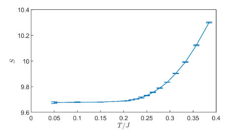
Figure 1: Entropy as a function of temperature for antiferromagnetic Ising model on the C60 lattice.

Anti-ferromagnetic Ising model.— To demonstrate the TIMC method’s precision, we applied it to the antiferromagnetic Ising model on both C60 and triangular lattices. The Hamiltonian is given by $H=J\sum_{\langle i,j\rangle}\hat{Z}_{i}\hat{Z}_{j}$, with $J>0$ indicating antiferromagnetic coupling and consideration given solely to nearest-neighbor interactions. We begin with the C60 lattice, composed of 12 pentagons and 20 hexagons. Frustration within the pentagons leads to a substantial ground state degeneracy for this model on the C60 lattice, quantified as 16,000 distinct states—a figure can be established via combinatorial analysis. The entropy temperature function derived from our TIMC method, as illustrated in Fig.1, is in excellent concordance with the analytical expectation that predicts a zero-temperature entropy of $\ln(16000)\approx 9.6803$. Our numerical results deliver an entropy value of $S=9.685\pm 0.011$, evidencing a remarkable consistency with theoretical predictions. Notably, the entropy value at $T/J=0.05$ closely approximates the residual entropy at zero temperature, attributable to a sizeable excitation gap on the order of $J$.

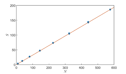
Figure 2: Entropy as a function of the lattice size of anti-ferromagnetic Ising model on the triangular lattice. Solid line: analytical solutions; Dots: Numerical results.

The triangular lattice serves as another prototypical example of geometric frustration. For the antiferromagnetic Ising model on such a lattice, the degree of ground state degeneracy is significantly higher. According to analytical exact solutions [27], this degeneracy escalates exponentially with the increase in system size, implying that entropy should similarly exhibit growth as a function of system size. The analytical calculation for the entropy per site is approximately 0.32307. Our TIMC method results, presented in Fig. 2, confirm this behavior: entropy indeed escalates with the system size $N$. The derived slope from our data yields an entropy per site value of $0.325\pm 0.002$, which is in close alignment with the exact analytical results. This not only substantiates the accuracy of the TIMC method but also its effectiveness in handling systems with extensive ground state degeneracy.

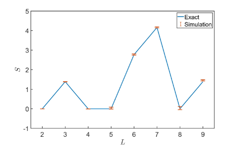
Figure 3: Entropy as a function of the lattice size of Newman-Moore spin glass model on the triangular lattice. Solid line: analytical solutions; Dots: numerical results.

The Newman-Moore Spin Glass Model.— The TIMC method’s versatility extends to the computation of residual entropy for spin glass models. For illustrative purposes, we focus on the Newman-Moore spin glass model [19]. The model’s Hamiltonian is expressed as

$$H=\frac{1}{2}J\sum_{i,j,k\text{ in }\bigtriangledown}\sigma_{i}\sigma_{j}\sigma_{k},$$ (8)

where each $\sigma_{i}$ takes a value of $\pm 1$. The summation is restricted to the interactions among three spins forming an inverted triangle on the triangular lattice. The ground state degeneracy of this model is exactly solvable, albeit through intricate mathematical methods [28]. Interestingly, the degeneracy does not follow a monotonic trend; rather, it oscillates with the system size. It has been established [19] that the model possesses a unique ground state when the system size is a power of two ($2^{k},k\in\text{Integer}$).

As depicted in Fig.3, our TIMC method’s computation of residual entropy across various system sizes aligns well with the analytical predictions, despite the complex nature of glassy systems. This underscores the TIMC method’s robustness and its potential as a reliable tool for probing the intricate landscapes of spin glasses.

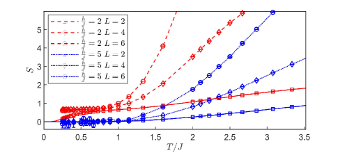
Figure 4: Entropy as a function of temperature of quantum Ising model. Comparing results of exact diagonalization and Monte Carlo calculation. Solid line: exact solutions; Dots and dashed lines: numerical results.

Quantum Ising model.— The TIMC method is equally adept at addressing quantum models, exemplified by our application to the quantum Ising model. We consider the ferromagnetic transverse field Ising model on a square lattice, as described by the Hamiltonian in Eq. (4). At zero temperature, this system undergoes a quantum phase transition from a ferromagnetic phase to a paramagnetic phase around the critical point $h/J\approx 3.04$. In the ferromagnetic phase, characterized by spontaneous $Z_{2}$-symmetry breaking, the ground state degeneracy is twofold. Conversely, in the paramagnetic phase, the transverse field aligns the spins in the $x$-direction, resulting in a non-degenerate ground state.

To substantiate these findings, we first juxtapose our TIMC outcomes with exact diagonalization results for a lattice size of $L=2$, as illustrated in Fig. 4. The data indicate that at high transverse field strengths, the residual entropy approaches zero at low temperatures, signaling a unique ground state. For a small transverse field ($h/J=2$), we observe an approximate $\ln 2$ entropy plateau, which diminishes at much lower temperatures due to finite size effects—on a finite lattice, the model’s ground state is invariably unique. As we reduce $h/J$ or increase the system size, the approximate $\ln 2$ plateau becomes more pronounced and extends closer to zero temperature, suggesting that it will persist in the thermodynamic limit. By applying the TIMC method to larger systems, we indeed observe that the approximate $\ln 2$ plateau extends to considerably lower temperatures as the system size increases.

Analyzing entropy as a function of temperature also allows for the precise calculation of specific heat using the formula $\frac{C_{V}}{T}=\left(\frac{\partial S}{\partial T}\right)_{V}$. This relationship is depicted in Fig.5. Notably, the specific heat exhibits a trend to diverge around the phase transition temperature $T_{c}/J\approx 2$ for $h/J=2$, an effect that becomes more pronounced with increasing system size. Such calculations underscore the value of entropy measurements in identifying and characterizing phase transitions.

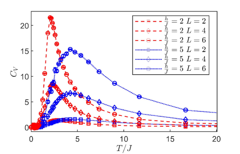
Figure 5: Specific heat as a function of temperature of quantum Ising model on the square lattice.

Conclusion and outlook.— In conclusion, our study has successfully demonstrated the robustness and versatility of the Temperature Incremental Monte Carlo (TIMC) method across a range of models, both classical and quantum. The TIMC method has proven itself as a powerful computational tool, capable of accurately calculating residual entropies in systems with varying degrees of ground state degeneracy.

For classical models, such as the antiferromagnetic Ising model on C60 and triangular lattices, the TIMC method not only confirmed the expected exponential increase in ground state degeneracy with system size but also provided entropy values in excellent agreement with analytical predictions. Similarly, in the context of spin glass models like the Newman-Moore model, the TIMC method adeptly navigated the oscillatory degeneracy behavior, offering results consistent with complex mathematical solutions.

In the quantum domain, our application of the TIMC method to the ferromagnetic transverse field Ising model on a square lattice provided insightful revelations into the nature of phase transitions. The method’s ability to distinguish between the unique ground state of the paramagnetic phase and the twofold degeneracy of the ferromagnetic phase at zero temperature—complemented by validation against exact diagonalization for small systems—highlights its precision and potential for broader applications.

Looking forward, the TIMC method holds promise for exploring more intricate classical and quantum systems, and could be adapted to tackle both fermionic and bosonic models. For example, it will be interesting to apply it to high dimensional fully or partially frustrated models [12, 29, 30]. Further, for the model with sign problem, the TIMC method can provide the entropy landscape at high temperature where the sign problem is not that severe, and thus may help to deduce possible phases in lower temperatures, for example, if there is any tendency to form superconductivity, the entropy will drop significantly.

The TIMC method’s success in handling extensive degeneracies and capturing critical phenomena at phase transitions opens up new avenues for investigating many-body systems. The potential applications of this method span a multitude of fields, from condensed matter physics to quantum information, where understanding entropy and ground state degeneracy is crucial.