An all-frequency stable surface integral equation algorithm for electromagnetism in 3-D unbounded penetrable media: Continuous and fully-discrete model analysis

Abstract

The simulation of electromagnetic waves that are induced by impinging incident waves in unbounded three-dimensional (3-D) penetrable media is fundamental for numerous applications. We use the time-harmonic Maxwell partial differential equations (PDEs) to model the wave propagation in 3-D space, which comprises a closed penetrable scatterer (with real or complex constant refractive index) and its unbounded free-space complement. Solving the continuous model to accurately simulate quantities of interest, such as the radar cross section (RCS) of the scatterer, is crucial for advances in electromagnetic-waves based technology. The RCS is a measure of electromagnetic far-fields, and exact surface-integral representations of the far-field can be obtained through unknown surface electromagnetic fields that are defined only on the bounded manifold interface separating the free-space and the scatterer. Surface integral equations (SIEs) that are equivalent to the time-harmonic Maxwell PDEs provide an efficient framework to directly model the surface electromagnetic fields and hence the RCS. The equivalent SIE system on the interface (with unknowns involving only surface fields) has the advantages that: (a) it avoids truncation of the unbounded region and the solution exactly satisfies the radiation condition; and (b) the surface-fields solution yields the unknowns in the Maxwell PDEs through surface potential representations of the interior and exterior fields. The Maxwell PDE system has been proven (several decades ago) to be stable for all frequencies, that is, (i) it does not possess eigenfrequencies (it is well-posed); and (ii) it does not suffer from low-frequency breakdowns (as the frequency approaches zero, it remains uniformly well-posed, and naturally decouples the electric and magnetic fields). However, weakly-singular SIE reformulations of the PDE satisfying these two properties, subject to a stabilization constraint, were derived and mathematically proven only about a decade ago (see J. Math. Anal. Appl. 412 (2014) 277-300, and related references therein). The aim of this article is two-fold: (I) To effect a robust coupling of the stabilization constraint to the weakly singular SIE and use mathematical analysis to establish that the resulting continuous weakly-singular second-kind self-adjoint SIE system (without constraints) retains all-frequency stability; and (II) To apply a fully-discrete spectral algorithm for the all-frequency-stable weakly-singular second-kind SIE, and prove spectral accuracy of the algorithm. We numerically demonstrate the high-order accuracy of the algorithm using several dielectric and absorbing benchmark scatterers with curved surfaces.

1 Introduction

Computation of the radar cross section (RCS) through simulation of electromagnetic waves in unbounded dielectric or absorbing penetrable media has been, and remains, crucial for advances in several technological and atmospheric science innovations [1, 2, 3, 4]. The classical approach to modeling the electric and magnetic fields in the presence of a penetrable body in free space is based on the Maxwell partial differential equations (PDEs), augmented with a radiation condition for the exterior fields, and tangential continuity of the electric field and magnetizing field across the interface [5, 6, 7].

The Maxwell system is uniquely solvable for all real and positive incident field frequencies when the media constants satisfy particular conditions (see [5, Theorem 2.1]). Our focus in this work is on time-harmonic electromagnetic waves with positive frequency $\omega$, characterized in a three dimensional piecewise-constant medium by the electric field ${\boldsymbol{\mathcal{E}}}$ and magnetic field ${\boldsymbol{\mathcal{H}}}$ [7, Page 178] with

$${\boldsymbol{\mathcal{E}}}(\boldsymbol{x},t)=\left\{\boldsymbol{E}(\boldsymbol{x})e^{-i\omega t}\right\},\quad{\boldsymbol{\mathcal{H}}}(\boldsymbol{x},t)=\left\{\boldsymbol{H}(\boldsymbol{x})e^{-i\omega t}\right\}.$$ (1)

We denote by $\partial D$ the closed-interface boundary of the domain $D\subset\mathbb{R}^{3}$, and write $D^{+}=\mathbb{R}^{3}\setminus\overline{D}$ and $D^{-}=D$ for the exterior and interior of the penetrable body respectively. We denote the permittivity and permeability constants in $D^{\pm}$ by $\epsilon^{\pm}$ and $\mu^{\pm}$ respectively, and assume that $\mu^{\pm}$ and $\epsilon^{+}$ are positive real numbers, whilst non-zero $\epsilon^{-}$ is positive real or complex, with non-negative real and imaginary part. It is convenient to then define

$$\epsilon(\boldsymbol{x})=\epsilon^{\pm},\qquad\mu(\boldsymbol{x})=\mu^{\pm},\qquad\mbox{for $\boldsymbol{x}\in D^{\pm}$}.$$ (2)

The refractive index of the medium is

$$\nu=\left(\frac{\mu^{-}\epsilon^{-}}{\mu^{+}\epsilon^{+}}\right)^{1/2},$$

and the penetrable media is called dielectric when $\nu$ is real, and absorbing otherwise (in which case it follows from the assumptions above that the imaginary part of $\nu$ is positive).

Interaction of an incident electromagnetic field with the penetrable body $D$ induces an interior field with spatial components $[\boldsymbol{E}^{-},\boldsymbol{H}^{-}]$ in $D^{-}$ and a scattered field with spatial components $[\boldsymbol{E}^{+},\boldsymbol{H}^{+}]$ in $D^{+}$. The spatial components $[\boldsymbol{E},\boldsymbol{H}]$ of the induced field, with

$$\boldsymbol{E}(\boldsymbol{x})=\boldsymbol{E}^{\pm}(\boldsymbol{x}),\qquad\boldsymbol{H}(\boldsymbol{x})=\boldsymbol{H}^{\pm}(\boldsymbol{x}),\qquad\qquad\boldsymbol{x}\in D^{\pm},$$ (3)

satisfy the time-harmonic Maxwell equations [7, Page 253]

$$\boldsymbol{\mathrm{curl}}\;\boldsymbol{E}(\boldsymbol{x})-\mathrm{i}\omega\mu(\boldsymbol{x})\boldsymbol{H}(\boldsymbol{x})=\boldsymbol{0},\qquad\boldsymbol{\mathrm{curl}}\;\boldsymbol{H}(\boldsymbol{x})+\mathrm{i}\omega\epsilon(\boldsymbol{x})\boldsymbol{E}(\boldsymbol{x})=\boldsymbol{0},\qquad\boldsymbol{x}\in D^{\pm},$$ (4)

and the Silver-Müller radiation condition

$$\lim_{|\boldsymbol{x}|\rightarrow\infty}\left[\sqrt{\mu^{+}}\boldsymbol{H}(\boldsymbol{x})\times\boldsymbol{x}-\sqrt{\epsilon^{+}}|\boldsymbol{x}|\boldsymbol{E}(\boldsymbol{x})\right]=\boldsymbol{0}.$$ (5)

The exterior and interior fields are induced by an incident electromagnetic field $[\boldsymbol{E}_{\mathrm{inc}},\boldsymbol{H}_{\mathrm{inc}}]$ impinging on the penetrable body. We require $[\boldsymbol{E}_{\mathrm{inc}},\boldsymbol{H}_{\mathrm{inc}}]$ to satisfy the homogeneous Maxwell equations

$$\boldsymbol{\mathrm{curl}}\;\boldsymbol{E}_{\mathrm{inc}}(\boldsymbol{x})-\mathrm{i}\omega\mu^{+}\boldsymbol{H}_{\mathrm{inc}}(\boldsymbol{x})=\boldsymbol{0},\quad\boldsymbol{\mathrm{curl}}\;\boldsymbol{H}_{\mathrm{inc}}(\boldsymbol{x})+\mathrm{i}\omega\epsilon^{+}\boldsymbol{E}_{\mathrm{inc}}(\boldsymbol{x})=\boldsymbol{0},\quad\boldsymbol{x}\in\mathbb{R}^{3}\setminus Q,$$ (6)

where $Q\subset\mathbb{R}^{3}$ is a compact or empty set, bounded away from the penetrable body $D$. In applications the incident wave is typically a plane wave, or a wave induced by a point source that satisfies (6). The total field is therefore $[\boldsymbol{E}_{\mathrm{tot}},\boldsymbol{H}_{\mathrm{tot}}]$ with

$$\boldsymbol{E}_{\mathrm{tot}}(\boldsymbol{x})=\boldsymbol{E}_{\mathrm{tot}}^{\pm}(\boldsymbol{x}),\qquad\boldsymbol{H}_{\mathrm{tot}}(\boldsymbol{x})=\boldsymbol{H}_{\mathrm{tot}}^{\pm}(\boldsymbol{x}),\qquad\qquad\boldsymbol{x}\in D^{\pm},$$ (7)

with

$$\boldsymbol{E}_{\mathrm{tot}}^{-}=\boldsymbol{E}^{-},\quad\boldsymbol{E}_{\mathrm{tot}}^{+}=\boldsymbol{E}^{+}+\boldsymbol{E}_{\mathrm{inc}},\quad\boldsymbol{H}_{\mathrm{tot}}^{-}=\boldsymbol{H}^{-},\quad\boldsymbol{H}_{\mathrm{tot}}^{+}=\boldsymbol{H}^{+}+\boldsymbol{H}_{\mathrm{inc}}.$$ (8)

We highlight that inside $D$ the total field is the induced field.

The tangential components of the total electric and magnetic fields are required to be continuous across the interface $\partial D$, leading to the interface conditions [7, Equation (5.6.66), Page 234]

$$\boldsymbol{E}^{-}_{\mathrm{tot}}\times\boldsymbol{n}=\boldsymbol{E}^{+}_{\mathrm{tot}}\times\boldsymbol{n},\qquad\boldsymbol{H}^{-}_{\mathrm{tot}}\times\boldsymbol{n}=\boldsymbol{H}^{+}_{\mathrm{tot}}\times\boldsymbol{n},\qquad\text{on $\partial D$},$$ (9)

where $\boldsymbol{n}$ is the outward unit normal to $\partial D$. A consequence of (4), (6), and (9) is that the normal components of the fields (called the surface charges) also satisfy interface conditions

$$\epsilon^{-}\boldsymbol{n}\cdot\boldsymbol{E}_{\mathrm{tot}}^{-}=\epsilon^{+}\boldsymbol{n}\cdot\boldsymbol{E}_{\mathrm{tot}}^{+},\qquad\mu^{-}\boldsymbol{n}\cdot\boldsymbol{H}_{\mathrm{tot}}^{-}=\mu^{+}\boldsymbol{n}\cdot\boldsymbol{H}_{\mathrm{tot}}^{+},\qquad\text{on $\partial D$}.$$ (10)

The scattered field $[\boldsymbol{E}^{+},\boldsymbol{H}^{+}]$ has the asymptotic behavior of an outgoing spherical wave [6, Theorem 6.8, Page 164], and in particular,

$$\boldsymbol{E}^{+}(\boldsymbol{x})=\frac{e^{\mathrm{i}k_{+}|\boldsymbol{x}|}}{|\boldsymbol{x}|}\left\{\boldsymbol{E}^{\infty}(\widehat{\boldsymbol{x}})+O\left(\frac{1}{|\boldsymbol{x}|}\right)\right\},$$ (11)

as $|\boldsymbol{x}|\rightarrow\infty$ uniformly in all directions $\widehat{\boldsymbol{x}}=\boldsymbol{x}/|\boldsymbol{x}|$, where $k_{+}=\omega\sqrt{\mu^{+}\epsilon^{+}}$ is the exterior wavenumber. The vector field $\boldsymbol{E}^{\infty}$ is known as the far field patterns of $\boldsymbol{E}^{+}$.

One way to solve the Maxwell PDE system given by (4)–(10) is to formulate equivalent surface integral equations (SIEs) on $\partial D$. The extensive survey in [8] reviews a century of research on deriving and using such SIEs. In previous work [9] we discussed different classes of SIE for the Maxwell dielectric problem and introduced our own original formulation which was an integral equation combined with a stabilization constraint. We showed that this formulation possesses a few remarkable properties that, taken together, are unique: first, this system is in the classical form of the identity plus a compact operator. Second, it does not suffer from spurious eigenfrequencies. Third, it does not suffer from the low-frequency breakdown phenomenon: as the frequency tends to zero, this system remains uniformly well posed. Fourth, the solution to this system is equal to the trace of the electric and magnetic fields on the interface. Points one to four were all proved in [9].

The main focus of this article is to implement the stabilization in such a way that a high-order numerical method can be developed, and prove spectral convergence of the numerical algorithm. To this end, one of the main issues is how to incorporate the stabilization into the integral equation formulation and retain an all-frequency stable uniquely-solvable system. One of the established approaches, as in the traditional combined-field formulation (combining the electric field integral equation (EFIE) and magnetic field integral equation (MFIE)), is to take a linear combination of the integral equation and the stabilization constraint. Such an approach has been used in the engineering literature [10, 11] without any proof that the uniquely solvable property is retained for all frequencies. We used such an approach for preliminary numerical investigations in [9] and demonstrated that, for spherical scatterers, there are some coupling parameters for which the unique solvability cannot be guaranteed for all frequencies. One of the key contributions in this present work is to establish, using robust mathematical proofs, that such a simple one-parameter coupling approach will lead to a non-uniquely solvable system for infinitely many choices of the parameters. Accordingly, using such a simple approach does not guarantee, in general, the key properties of the all-frequency stable integral equation formulation, subject to the constraint.

Subsequently, in this article we introduce a new continuous formulation that incorporates the constraint efficiently into one equation, and we prove that the established unique solution, with the constraint, is equivalent to the solution obtained using our new coupled formulation. The main focus of this paper is to apply a high-order numerical algorithm for the new symmetric formulation, and prove spectrally accurate convergence under certain conditions that are especially suited for curved interfaces. We substantiate our robust mathematical results with numerical experiments. The underlying spectrally-accurate numerical framework was developed for perfect conductors in [12] and subsequently further developed for the dielectric model in [13], where we incorporated the constraint using a complicated saddle-point formulation. Numerical analysis of such a saddle-point approach is yet to be explored. The present article is the first work in the literature to develop numerical analysis for an all-frequency stable and uniquely solvable weakly-singular SIE system.

The rest of this article is as follows. In Section 2 we first review properties of surface integral operators that are relevant to this study. We then review an all-frequency stable surface integral equation subject to a stabilization constraint, and a main result from [9] in Section 3. In Appendix A we prove that the simple approach of combining the integral equation with the stabilization constraint using a single parameter does not, in general, guarantee unique solvability of the resulting system, for infinitely many choices of the parameters. Motivated by this, in Section 4 we introduce a new equivalent formulation incorporating the stabilization constraint in a self-adjoint form and prove that the new single-equation system, without any constraint, is uniquely solvable. In Section 5 we introduce a fully-discrete numerical scheme for our new single-equation weakly-singular SIE system and prove that the associated numerical solution converges super-algebraically. In Section 6 we implement the spectrally accurate algorithm and demonstrate the superalgebraic convergence for a class of convex and non-convex test obstacles that are widely used in the literature.

2 Surface integral operators and properties

In this section we introduce the integral operators that subsequently appear in our SIE. The starting point is the use of particular potentials and their traces onto the interface $\partial D$. We use the same notation as in our previous article [9] and we first recall from [9] some notation and definitions. For related derivations and proofs, we refer to [9].

Let $\Omega\subseteq\mathbb{R}^{3}$ be either $D^{-}$, $D^{+}$, $\partial D$ or $\mathbb{R}^{3}$. For a non-negative integer $m$ and $\sigma\in\mathbb{R}$ with $0<\sigma\leq 1$, let $\mathrm{C}^{m}(\overline{\Omega})$ denote the standard space of $m$-times continuously differentiable functions and $\mathrm{C}^{m,\sigma}(\overline{\Omega})$ denote the Hölder space of all functions in $\mathrm{C}^{m}(\overline{\Omega})$ whose derivatives of order $m$ are uniformly Hölder continuous with exponent $\sigma$. For $s\in\mathbb{R}$ and bounded $\Omega$ the space $\mathrm{H}^{s}(\Omega)$ is the standard Sobolev space of order $s$.

The vector-valued counterparts of these spaces will be denoted by boldface symbols. Thus, for $m\in\mathbb{N},\;s\in\mathbb{R},0\leq\sigma\leq 1$,

$$\boldsymbol{\mathrm{C}}^{m,\sigma}(\overline{\Omega})=\Big{[}\mathrm{C}^{m,\sigma}(\overline{\Omega})\Big{]}^{3},\quad\boldsymbol{\mathrm{H}}^{s}(\Omega)=\Big{[}\mathrm{H}^{s}(\Omega)\Big{]}^{3}.$$ (12)

Let $\boldsymbol{\gamma}^{\pm}$ be the standard exterior/interior trace operator defined for a continuous vector field $\boldsymbol{u}$ on $\overline{D^{\pm}}$ as

$$\Big{(}\boldsymbol{\gamma}^{\pm}\boldsymbol{u}\Big{)}(\boldsymbol{x})=\lim_{h\rightarrow 0^{\pm}}\boldsymbol{u}(\boldsymbol{x}+h\boldsymbol{n}(\boldsymbol{x})),\qquad\boldsymbol{x}\in\partial D.$$ (13)

Let $\boldsymbol{\gamma}_{\boldsymbol{t}}^{\pm},\gamma_{\boldsymbol{n}}^{\pm}$ be respectively the (twisted) tangential and normal trace operators, defined for a continuous vector field $\boldsymbol{u}$ on $\overline{D^{\pm}}$ as

$$\boldsymbol{\gamma}_{\boldsymbol{t}}^{\pm}\boldsymbol{u}=(\boldsymbol{\gamma}^{\pm}\boldsymbol{u})\times\boldsymbol{n}.\qquad\gamma_{\boldsymbol{n}}^{\pm}\boldsymbol{u}=(\boldsymbol{\gamma}^{\pm}\boldsymbol{u})\cdot\boldsymbol{n}.$$ (14)

We denote by $\boldsymbol{\mathrm{C}}_{\boldsymbol{t}}^{m,\sigma}(\partial D)$ and $\boldsymbol{\mathrm{H}}^{s}_{\boldsymbol{t}}(\partial D)$ respectively the spaces of tangential vector fields on $\partial D$ with regularity $\boldsymbol{\mathrm{C}}^{m,\sigma}$ and $\boldsymbol{\mathrm{H}}^{s}$.

Let

$$G_{\pm}(\boldsymbol{x},\boldsymbol{y})=\frac{1}{4\pi}\frac{e^{\mathrm{i}k_{\pm}|\boldsymbol{x}-\boldsymbol{y}|}}{|\boldsymbol{x}-\boldsymbol{y}|},$$ (15)

where $k_{\pm}=\omega\sqrt{\epsilon^{\pm}\mu^{\pm}}$ denotes the exterior and interior wavenumber respectively. Let $\Psi^{V}_{\pm}$ and $\underline{\boldsymbol{\Psi}}^{\boldsymbol{V}}_{\pm}$ be respectively the scalar and vector single layer potential operators, defined for scalar and vector surface densities $w$ and $\boldsymbol{w}$ as

$$(\Psi^{V}_{\pm}w)(\boldsymbol{x})=\int_{\partial D}G_{\pm}(\boldsymbol{x},\boldsymbol{y})\;w(\boldsymbol{y})\;ds(\boldsymbol{y}),\quad(\underline{\boldsymbol{\Psi}}^{\boldsymbol{V}}_{\pm}\boldsymbol{w})(\boldsymbol{x})=\int_{\partial D}G_{\pm}(\boldsymbol{x},\boldsymbol{y})\;\boldsymbol{w}(\boldsymbol{y})\;ds(\boldsymbol{y}),$$ (16)

for $\boldsymbol{x}\in\mathbb{R}^{3}\setminus\partial D$. We assume that the surface $\partial D$ is at least of class $\mathrm{C}^{m^{*},1}$, for some integer $m^{*}\geq 1$. Then the operators $\Psi^{V}_{\pm}:\mathrm{C}(\partial D)\rightarrow\mathrm{C}^{0,\alpha}(\mathbb{R}^{3})$ and, for $0<\alpha<1$, $\underline{\boldsymbol{\Psi}}^{V}_{\pm}:\boldsymbol{\mathrm{C}}(\partial D)\rightarrow\boldsymbol{\mathrm{C}}^{0,\alpha}(\mathbb{R}^{3})$ are bounded linear operators [6, Theorems 3.3, 6.12]. Hence $\boldsymbol{\gamma}_{\boldsymbol{t}}^{\pm}\circ\underline{\boldsymbol{\Psi}}^{\boldsymbol{V}}_{\pm}:\boldsymbol{\mathrm{C}}(\partial D)\rightarrow\boldsymbol{\mathrm{C}}_{\boldsymbol{t}}^{0,\alpha}(\partial D)$ is a bounded linear operator and consequently compact as an operator onto $\boldsymbol{\mathrm{C}}(\partial D)$ because of the compact imbedding [6, Theorem 3.2]. Similarly, using the properties of the single layer potential on Sobolev spaces (see [14, Theorem 1(i)]), $\boldsymbol{\gamma}_{\boldsymbol{t}}^{\pm}\circ\underline{\boldsymbol{\Psi}}^{\boldsymbol{V}}_{\pm}$ is a compact operator onto $\boldsymbol{\mathrm{H}}^{\frac{1}{2}}(\partial D)$. Using the jump relation for the single layer potential [6, 7], we obtain

$$\boldsymbol{\gamma}_{\boldsymbol{t}}^{\pm}\circ\underline{\boldsymbol{\Psi}}^{\boldsymbol{V}}_{\pm}\boldsymbol{w}=\underline{\boldsymbol{\mathscr{A}}}_{\pm}\boldsymbol{w},\qquad\gamma_{\boldsymbol{n}}^{\pm}\circ\underline{\boldsymbol{\Psi}}^{\boldsymbol{V}}_{\pm}\boldsymbol{w}={{\mathscr{F}}}_{\pm}\boldsymbol{w},$$ (17)

where the tangential-field-valued and scalar-valued operators are defined as

$$(\underline{\boldsymbol{\mathscr{A}}}_{\pm}\boldsymbol{w})(\boldsymbol{x}) = \int_{\partial D}G_{\pm}(\boldsymbol{x},\boldsymbol{y})\;\boldsymbol{w}(\boldsymbol{y})\times\boldsymbol{n}(\boldsymbol{x})\;ds(\boldsymbol{y}),\qquad\boldsymbol{x}\in\partial D,$$ (18)

$$({{\mathscr{F}}}_{\pm}\boldsymbol{w})(\boldsymbol{x}) = \int_{\partial D}G_{\pm}(\boldsymbol{x},\boldsymbol{y})\;\boldsymbol{w}(\boldsymbol{y})\cdot\boldsymbol{n}(\boldsymbol{x})\;ds(\boldsymbol{y}),\qquad\boldsymbol{x}\in\partial D.$$ (19)

It is useful to consider the normal-field operator

$$(\boldsymbol{n}{{\mathscr{F}}}_{\pm}\boldsymbol{w})(\boldsymbol{x})=\boldsymbol{n}(\boldsymbol{x})({{\mathscr{F}}}_{\pm}\boldsymbol{w})(\boldsymbol{x}),\qquad\boldsymbol{x}\in\partial D.$$ (20)

The surface integral operators $\underline{\boldsymbol{\mathscr{A}}}_{\pm}$ and $\boldsymbol{n}{{\mathscr{F}}}_{\pm}$ are compact as operators on $\boldsymbol{\mathrm{C}}(\partial D)$ and $\boldsymbol{\mathrm{H}}^{\frac{1}{2}}(\partial D)$. Further, for $\alpha$, $s$ and integer $m$ satisfying

$$0<\alpha<1,\qquad 0\leq m<m^{*},\qquad 0<s\leq m^{*},$$ (21)

we have that

$$\underline{\boldsymbol{\mathscr{A}}}_{\pm},\boldsymbol{n}{{\mathscr{F}}}_{\pm}:\boldsymbol{\mathrm{C}}^{m}(\partial D)\rightarrow\boldsymbol{\mathrm{C}}^{m,\alpha}(\partial D),\qquad\qquad\underline{\boldsymbol{\mathscr{A}}}_{\pm},\boldsymbol{n}{{\mathscr{F}}}_{\pm}:\boldsymbol{\mathrm{H}}^{s-1}(\partial D)\rightarrow\boldsymbol{\mathrm{H}}^{s}(\partial D),$$ (22)

are bounded linear operators. The operators in (18)–(20) enjoy these smoothing (and hence compactness) properties essentially because the kernels of these surface integral operators are weakly-singular.

We define vector-valued surface integral operators

$$(\underline{\boldsymbol{\mathscr{B}}}_{\pm}w)(\boldsymbol{x}) = \int_{\partial D}\boldsymbol{\mathrm{grad}}_{\boldsymbol{x}}G_{\pm}(\boldsymbol{x},\boldsymbol{y})\times\boldsymbol{n}(\boldsymbol{x})\;w(\boldsymbol{y})\;ds(\boldsymbol{y}),$$ (23)

$$(\underline{\boldsymbol{\mathscr{C}}}_{\pm}\boldsymbol{w})(\boldsymbol{x}) = -\boldsymbol{n}(\boldsymbol{x})\times\boldsymbol{\mathrm{curl}}_{\boldsymbol{x}}\int_{\partial D}G_{\pm}(\boldsymbol{x},\boldsymbol{y})\boldsymbol{w}(\boldsymbol{y})\;ds(\boldsymbol{y}),$$ (24)

for $\boldsymbol{x}\in\partial D$, and related scalar-valued surface integral operators

$$({{\mathscr{G}}}_{\pm}w)(\boldsymbol{x}) = \int_{\partial D}\frac{\partial G_{\pm}}{\partial\boldsymbol{n}(\boldsymbol{x})}(\boldsymbol{x},\boldsymbol{y})\;w(\boldsymbol{y})\;ds(\boldsymbol{y}),$$ (25)

$$({{\mathscr{H}}}_{\pm}\boldsymbol{w})(\boldsymbol{x}) = \int_{\partial D}\Big{(}\boldsymbol{\mathrm{grad}}_{\boldsymbol{x}}G_{\pm}(\boldsymbol{x},\boldsymbol{y})\times\boldsymbol{n}(\boldsymbol{x})\Big{)}\cdot\boldsymbol{w}(\boldsymbol{y})\;ds(\boldsymbol{y}).$$ (26)

We note that for a tangential density $\boldsymbol{w}$,

$$(\underline{\boldsymbol{\mathscr{C}}}_{\pm}\boldsymbol{w})(\boldsymbol{x})=(\underline{\boldsymbol{\mathscr{D}}}_{\pm}\boldsymbol{w})(\boldsymbol{x})-(\underline{\boldsymbol{\mathscr{E}}}_{\pm}\boldsymbol{w})(\boldsymbol{x}),$$ (27)

where for $\boldsymbol{x}\in\partial D$,

$$(\underline{\boldsymbol{\mathscr{D}}}_{\pm}\boldsymbol{w})(\boldsymbol{x}) = \int_{\partial D}\frac{\partial G_{\pm}}{\partial\boldsymbol{n}(\boldsymbol{x})}(\boldsymbol{x},\boldsymbol{y})\;\boldsymbol{w}(\boldsymbol{y})\;ds(\boldsymbol{y}),$$ (28)

$$(\underline{\boldsymbol{\mathscr{E}}}_{\pm}\boldsymbol{w})(\boldsymbol{x}) = \int_{\partial D}\Big{(}\boldsymbol{\mathrm{grad}}_{\boldsymbol{x}}G_{\pm}(\boldsymbol{x},\boldsymbol{y})\Big{)}\;\boldsymbol{w}(\boldsymbol{y})\cdot\Big{(}\boldsymbol{n}(\boldsymbol{x})-\boldsymbol{n}(\boldsymbol{y})\Big{)}\;ds(\boldsymbol{y}).$$ (29)

It is also useful to consider the normal field surface integral operators

$$(\boldsymbol{n}{{\mathscr{G}}}_{\pm}w)(\boldsymbol{x})=\boldsymbol{n}(\boldsymbol{x})({{\mathscr{G}}}_{\pm}w)(\boldsymbol{x}),\qquad(\boldsymbol{n}{{\mathscr{H}}}_{\pm}\boldsymbol{w})(\boldsymbol{x})=\boldsymbol{n}(\boldsymbol{x})({{\mathscr{H}}}_{\pm}\boldsymbol{w})(\boldsymbol{x}),\qquad\boldsymbol{x}\in\partial D.$$ (30)

Clearly, the kernels of the surface integral operators $\underline{\boldsymbol{\mathscr{D}}}_{\pm}$ and ${{\mathscr{G}}}_{\pm}$ are weakly-singular. Hence ${{\mathscr{G}}}_{\pm}$ is a compact operator on $\mathrm{C}(\partial D)$ and $\mathrm{H}^{\frac{1}{2}}(\partial D)$.

Since $\partial D$ is of at least $\mathrm{C}^{1,1}$-class, we obtain

$$|\boldsymbol{n}(\boldsymbol{x})-\boldsymbol{n}(\boldsymbol{y})|\leq C|\boldsymbol{x}-\boldsymbol{y}|,\qquad\boldsymbol{x},\boldsymbol{y}\in\partial D,$$ (31)

for some constant $C$ that depends on the geometry of $\partial D$. Thus, because of the term $\boldsymbol{n}(\boldsymbol{x})-\boldsymbol{n}(\boldsymbol{y})$ in (29), the operator $\underline{\boldsymbol{\mathscr{E}}}_{\pm}$ is weakly-singular. Hence $\underline{\boldsymbol{\mathscr{C}}}_{\pm}$ is a compact operator on $\boldsymbol{\mathrm{C}}_{\boldsymbol{t}}(\partial D)$ and $\boldsymbol{\mathrm{H}}^{\frac{1}{2}}_{\boldsymbol{t}}(\partial D)$. In addition, if (21) holds then

$$\underline{\boldsymbol{\mathscr{C}}}_{\pm}:\boldsymbol{\mathrm{C}}^{m}_{\boldsymbol{t}}(\partial D)\rightarrow\boldsymbol{\mathrm{C}}^{m,\alpha}_{\boldsymbol{t}}(\partial D),\qquad\underline{\boldsymbol{\mathscr{C}}}_{\pm}:\boldsymbol{\mathrm{H}}^{s-1}_{\boldsymbol{t}}(\partial D)\rightarrow\boldsymbol{\mathrm{H}}^{s}_{\boldsymbol{t}}(\partial D),$$

$${{\mathscr{G}}}_{\pm}:\mathrm{C}^{m}(\partial D)\rightarrow\mathrm{C}^{m,\alpha}(\partial D),\qquad{{\mathscr{G}}}_{\pm}:\mathrm{H}^{s-1}(\partial D)\rightarrow\mathrm{H}^{s}(\partial D),$$

are bounded linear operators. The kernels of the surface integral operators $\underline{\boldsymbol{\mathscr{B}}}_{\pm},{{\mathscr{H}}}_{\pm}$ in (23), (26) have order $1/r^{2}$ singularity. However, our reformulation of the time-harmonic dielectric model requires only operators $\underline{\boldsymbol{\mathscr{B}}}_{+}-\underline{\boldsymbol{\mathscr{B}}}_{-}$ and ${{\mathscr{H}}}_{+}-{{\mathscr{H}}}_{-}$. It follows from [15, Remark 3.1.3] that $\underline{\boldsymbol{\mathscr{B}}}_{+}-\underline{\boldsymbol{\mathscr{B}}}_{-}$ and ${{\mathscr{H}}}_{+}-{{\mathscr{H}}}_{-}$ have weakly-singular kernels. Thus the operator $\boldsymbol{n}{{\mathscr{H}}}_{+}-\boldsymbol{n}{{\mathscr{H}}}_{-}$ is compact on $\boldsymbol{\mathrm{C}}(\partial D)$ and $\boldsymbol{\mathrm{H}}^{\frac{1}{2}}(\partial D)$ whilst the operator $\underline{\boldsymbol{\mathscr{B}}}_{+}-\underline{\boldsymbol{\mathscr{B}}}_{-}$ is compact on $\mathrm{C}(\partial D)$ and $\mathrm{H}^{\frac{1}{2}}(\partial D)$, and if (21) holds then the following linear operators are bounded:

$$\boldsymbol{n}{{\mathscr{H}}}_{+}-\boldsymbol{n}{{\mathscr{H}}}_{-}:\boldsymbol{\mathrm{C}}^{m}(\partial D)\rightarrow\boldsymbol{\mathrm{C}}^{m,\alpha}(\partial D),\qquad\boldsymbol{n}{{\mathscr{H}}}_{+}-\boldsymbol{n}{{\mathscr{H}}}_{-}:\boldsymbol{\mathrm{H}}^{s-1}(\partial D)\rightarrow\boldsymbol{\mathrm{H}}^{s}(\partial D),$$

$$\underline{\boldsymbol{\mathscr{B}}}_{+}-\underline{\boldsymbol{\mathscr{B}}}_{-}:\mathrm{C}^{m}(\partial D)\rightarrow\boldsymbol{\mathrm{C}}^{m,\alpha}(\partial D),\qquad\qquad\underline{\boldsymbol{\mathscr{B}}}_{+}-\underline{\boldsymbol{\mathscr{B}}}_{-}:\mathrm{H}^{s-1}(\partial D)\rightarrow\boldsymbol{\mathrm{H}}^{s}(\partial D).$$

Furthermore, we define two further scalar integral operators that we use in our additional scalar integral equations for indirectly imposing the identities connecting currents and charges,

$$({{\mathscr{S}}}_{\pm}w)(\boldsymbol{x}) = \int_{\partial D}G_{\pm}(\boldsymbol{x},\boldsymbol{y})\;w(\boldsymbol{y})\;ds(\boldsymbol{y}),\quad\boldsymbol{x}\in\partial D,$$ (32)

$$({{\mathscr{K}}}_{\pm}\boldsymbol{w})(\boldsymbol{x}) = \int_{\partial D}\Big{(}\boldsymbol{\mathrm{grad}}_{\boldsymbol{x}}G_{\pm}(\boldsymbol{x},\boldsymbol{y})\times\boldsymbol{n}(\boldsymbol{y})\Big{)}\cdot\boldsymbol{w}(\boldsymbol{y})\;ds(\boldsymbol{y}),\quad\boldsymbol{x}\in\partial D.$$ (33)

The operator ${{\mathscr{S}}}_{+}-{{\mathscr{S}}}_{-}$ is compact on $\mathrm{C}(\partial D)$ and $\mathrm{H}^{\frac{1}{2}}(\partial D)$ whilst the operator ${{\mathscr{K}}}_{+}-{{\mathscr{K}}}_{-}$ is compact on $\boldsymbol{\mathrm{C}}(\partial D)$ and $\boldsymbol{\mathrm{H}}^{\frac{1}{2}}(\partial D)$, and if (21) holds then the following linear operators are bounded:

$${{\mathscr{S}}}_{+}-{{\mathscr{S}}}_{-}:\mathrm{C}^{m}(\partial D)\rightarrow\mathrm{C}^{m,\alpha}(\partial D),\qquad{{\mathscr{S}}}_{+}-{{\mathscr{S}}}_{-}:\mathrm{H}^{s-1}(\partial D)\rightarrow\mathrm{H}^{s}(\partial D),$$

$${{\mathscr{K}}}_{+}-{{\mathscr{K}}}_{-}:\boldsymbol{\mathrm{C}}^{m}(\partial D)\rightarrow\mathrm{C}^{m,\alpha}(\partial D),\quad{{\mathscr{K}}}_{+}-{{\mathscr{K}}}_{-}:\boldsymbol{\mathrm{H}}^{s-1}(\partial D)\rightarrow\mathrm{H}^{s}(\partial D).$$

Finally, we introduce the following weakly-singular operators to facilitate recalling in the next section our first second-kind surface-integral system that is all-frequency-stable subject to a stability constraint.

$$\widetilde{\underline{\boldsymbol{\mathscr{C}}}}^{(\alpha^{+},\alpha^{-})} = \alpha^{+}\underline{\boldsymbol{\mathscr{C}}}_{+}-\alpha^{-}\underline{\boldsymbol{\mathscr{C}}}_{-},\qquad\widetilde{\underline{\boldsymbol{\mathscr{A}}}}^{(\alpha^{+},\alpha^{-},\beta^{+},\beta^{-},\lambda)}=\mathrm{i}\lambda(\beta^{+}\alpha^{+}\underline{\boldsymbol{\mathscr{A}}}_{+}-\beta^{-}\alpha^{-}\underline{\boldsymbol{\mathscr{A}}}_{-}),$$

$$\widetilde{{{\mathscr{G}}}}^{(\alpha^{+},\alpha^{-})} = {{\mathscr{G}}}_{+}-\frac{\alpha^{+}}{\alpha^{-}}{{\mathscr{G}}}_{-},\qquad\widetilde{{{\mathscr{F}}}}^{(\alpha^{+},\alpha^{-},\lambda)}=\mathrm{i}\lambda\left(\alpha^{+}{{\mathscr{F}}}_{+}-\alpha^{-}{{\mathscr{F}}}_{-}\right),$$

$$\widetilde{\underline{\boldsymbol{\mathscr{B}}}}=\underline{\boldsymbol{\mathscr{B}}}_{+} - \underline{\boldsymbol{\mathscr{B}}}_{-},\qquad\widetilde{{{\mathscr{H}}}}={{\mathscr{H}}}_{+}-{{\mathscr{H}}}_{-},\quad\widetilde{{{\mathscr{S}}}}=({{\mathscr{S}}}_{+}-{{\mathscr{S}}}_{-}),\quad\widetilde{{{\mathscr{K}}}}=({{\mathscr{K}}}_{+}-{{\mathscr{K}}}_{-}).$$ (34)

In this notation, when it is used subsequently, the parameter $\lambda$ will be replaced by $\pm\omega$ and hence $\widetilde{\underline{\boldsymbol{\mathscr{A}}}}^{(\alpha^{+},\alpha^{-},\beta^{+},\beta^{-},\pm\omega)}$ and $\widetilde{{{\mathscr{F}}}}^{(\alpha^{+},\alpha^{-},\pm\omega)}$ tend to zero operators as $\omega\rightarrow 0$.

3 A stability constrained well-posed SIE system

In this section we recall from [9] a matrix-operator operator and a stability constraint, and hence, subject to the constraint, an all-frequency-stable weakly-singular SIE system that is equivalent to the Maxwell PDE. To this end, let $\boldsymbol{\mathbb{M}}$ be the $2\times 2$ weakly-singular operator

$$\boldsymbol{\mathbb{M}}=\left[\begin{array}[]{ll}\boldsymbol{\mathcal{M}}^{(\epsilon^{+},\epsilon^{-})}&\boldsymbol{\mathcal{N}}^{(\epsilon^{+},\epsilon^{-},\mu^{+},\mu^{-},\omega)}\\ \\ \boldsymbol{\mathcal{N}}^{(\mu^{+},\mu^{-},\epsilon^{+},\epsilon^{-},-\omega)}&\boldsymbol{\mathcal{M}}^{(\mu^{+},\mu^{-})}\end{array}\right],$$ (35)

with

$$\boldsymbol{\mathcal{M}}^{(\alpha^{+},\alpha^{-})}\boldsymbol{w} = \frac{2}{\alpha^{+}+\alpha^{-}}\Bigg{\{}\boldsymbol{n}\times\left[\widetilde{}\underline{\boldsymbol{\mathscr{C}}}^{(\alpha^{+},\alpha^{-})}(\boldsymbol{w}\times\boldsymbol{n})+\alpha^{+}\widetilde{}\underline{\boldsymbol{\mathscr{B}}}^{(\alpha^{+},\alpha^{-})}(\boldsymbol{w}\cdot\boldsymbol{n})\right]$$ (36)

$$\hskip 65.04256pt-\alpha^{-}\boldsymbol{n}\left[\widetilde{{\mathscr{H}}}(\boldsymbol{w}\times\boldsymbol{n})-\widetilde{{\mathscr{G}}}^{(\alpha^{+},\alpha^{-})}(\boldsymbol{w}\cdot\boldsymbol{n})\right]\Bigg{\}},$$

$$\boldsymbol{\mathcal{N}}^{(\alpha^{+},\alpha^{-},\beta^{+},\beta^{-},\lambda)}\boldsymbol{w}=\frac{2}{\alpha^{+}+\alpha^{-}}\left\{\left[\boldsymbol{n}\times\widetilde{}\underline{\boldsymbol{\mathscr{A}}}^{(\alpha^{+},\alpha^{-},\beta^{+},\beta^{-},\lambda)}+\alpha^{-}\boldsymbol{n}\widetilde{{\mathscr{F}}}^{(\beta_{+},\beta_{-},\lambda)}\right](\boldsymbol{w}\times\boldsymbol{n})\right\}.$$ (37)

It is easy to see the important property of $\boldsymbol{\mathbb{M}}$ that in the limit $\omega\rightarrow 0$, the off-diagonal entries of $\boldsymbol{\mathbb{M}}$ are zero, and hence the resulting diagonal operator facilitates decoupling of the electric and magnetic fields as $\omega\rightarrow 0$. We further observe that, because of the weak singularity of their kernels, $\boldsymbol{\mathcal{M}}^{(\alpha_{+},\alpha_{-})}$ and $\boldsymbol{\mathcal{N}}^{(\alpha_{+},\alpha_{-},\beta_{+},\beta_{-},\lambda)}$ defined in (36)–(37) are compact as operators on $X$,$\boldsymbol{\mathrm{C}}(\partial D)$ and on $\boldsymbol{\mathrm{H}}^{\frac{1}{2}}(\partial D)$. Furthermore, for $\alpha$, $m$ and $s$ satisfying (21),

$$\boldsymbol{\mathcal{M}}^{(\alpha_{+},\alpha_{-})},\boldsymbol{\mathcal{N}}^{(\alpha_{+},\alpha_{-},\beta_{+},\beta_{-},\lambda)} : \boldsymbol{\mathrm{C}}^{m}(\partial D)\rightarrow\boldsymbol{\mathrm{C}}^{m,\alpha}(\partial D),$$

$$\boldsymbol{\mathcal{M}}^{(\alpha_{+},\alpha_{-})},\boldsymbol{\mathcal{N}}^{(\alpha_{+},\alpha_{-},\beta_{+},\beta_{-},\lambda)} : \boldsymbol{\mathrm{H}}^{s-1}(\partial D)\rightarrow\boldsymbol{\mathrm{H}}^{s}(\partial D),$$

are bounded linear operators. Consequently the $2\times 2$ matrix operator $\boldsymbol{\mathbb{M}}$ defined in (35) is a compact operator on $\boldsymbol{\mathrm{C}}(\partial D)\times\boldsymbol{\mathrm{C}}(\partial D)$ and on $\boldsymbol{\mathrm{H}}^{\frac{1}{2}}(\partial D)\times\boldsymbol{\mathrm{H}}^{\frac{1}{2}}(\partial D)$. In addition, if (21) holds then

$$\boldsymbol{\mathbb{M}} : \boldsymbol{\mathrm{C}}^{m}(\partial D)\times\boldsymbol{\mathrm{C}}^{m}(\partial D)\rightarrow\boldsymbol{\mathrm{C}}^{m,\alpha}(\partial D)\times\boldsymbol{\mathrm{C}}^{m,\alpha}(\partial D),$$ (38)

$$\boldsymbol{\mathbb{M}} : \boldsymbol{\mathrm{H}}^{s-1}(\partial D)\times\boldsymbol{\mathrm{H}}^{s-1}(\partial D)\rightarrow\boldsymbol{\mathrm{H}}^{s}(\partial D)\times\boldsymbol{\mathrm{H}}^{s}(\partial D),$$ (39)

are bounded linear operators. For $\boldsymbol{x}\in\partial D$ define,

$$\boldsymbol{e}^{\mathrm{i}}(\boldsymbol{x}) = \frac{2\epsilon^{+}}{\epsilon^{+}+\epsilon^{-}}\boldsymbol{n}(\boldsymbol{x})\times\left(\boldsymbol{\gamma}_{\boldsymbol{t}}^{+}\boldsymbol{E}_{\mathrm{i}}\right)(\boldsymbol{x})+\frac{2\epsilon^{-}}{\epsilon^{+}+\epsilon^{-}}\boldsymbol{n}(\boldsymbol{x})\left(\gamma_{\boldsymbol{n}}^{+}\boldsymbol{E}_{\mathrm{i}}\right)(\boldsymbol{x}),$$ (40)

$$\boldsymbol{h}^{\mathrm{i}}(\boldsymbol{x}) = \frac{2\mu^{+}}{\mu^{+}+\mu^{-}}\boldsymbol{n}(\boldsymbol{x})\times\left(\boldsymbol{\gamma}_{\boldsymbol{t}}^{+}\boldsymbol{H}_{\mathrm{i}}\right)(\boldsymbol{x})+\frac{2\mu^{-}}{\mu^{+}+\mu^{-}}\boldsymbol{n}(\boldsymbol{x})\left(\gamma_{\boldsymbol{n}}^{+}\boldsymbol{H}_{\mathrm{i}}\right)(\boldsymbol{x}),$$ (41)

where $[\boldsymbol{E}_{\mathrm{i}},\boldsymbol{H}_{\mathrm{i}}]$ is an incident electromagnetic wave. In [9] we proved that if $(\boldsymbol{f},\boldsymbol{g})^{T}=(\boldsymbol{E}_{\mathrm{i}}|_{\partial D},\boldsymbol{H}_{\mathrm{i}}|_{\partial D})^{T}$ and $(\boldsymbol{e},\boldsymbol{h})^{T}$ is the exterior trace of the total field solving the Maxwell dielectric problem (4)–(10) for the same incident field $[\boldsymbol{E}_{\mathrm{i}},\boldsymbol{H}_{\mathrm{i}}]$, then

$$\Big{[}\boldsymbol{\mathbb{I}}+\boldsymbol{\mathbb{M}}\Big{]}\left(\begin{array}[]{l}\boldsymbol{e}\\ \boldsymbol{h}\end{array}\right)=\left(\begin{array}[]{l}\boldsymbol{f}\\ \boldsymbol{g}\end{array}\right),$$ (42)

where $\boldsymbol{\mathbb{I}}$ is the block identity operator. This holds for all frequencies $\omega>0$. However, the system (42) may become singular for some frequencies $\omega$. In [9] we found a constraint such that equation (42) augmented by that constraint is uniquely solvable for all frequencies. The stability constraint, which actually uses just scalar operators that are also used in acoustics, is governed by the operator $\boldsymbol{\mathbb{J}}$ defined (with the same domain and range spaces as $\boldsymbol{\mathbb{M}}$) as:

$$\boldsymbol{\mathbb{J}}\left(\begin{array}[]{l}\widetilde{\boldsymbol{e}}\\ \widetilde{\boldsymbol{h}}\end{array}\right)=\left(0,~{}0,~{}\widetilde{{{\mathscr{K}}}}\widetilde{\boldsymbol{e}}+\mathrm{i}\omega\mu^{+}\widetilde{{{\mathscr{S}}}}(\widetilde{\boldsymbol{h}}\cdot\boldsymbol{n}),~{}0,~{}0,~{}\widetilde{{{\mathscr{K}}}}\widetilde{\boldsymbol{h}}-\mathrm{i}\omega\epsilon^{+}\widetilde{{{\mathscr{S}}}}(\widetilde{\boldsymbol{e}}\cdot\boldsymbol{n})\right)^{T}.$$ (43)

For $\alpha$, $m$ and $s$ satisfying (21),

$$\boldsymbol{\mathbb{J}} : \boldsymbol{\mathrm{C}}^{m}(\partial D)\times\boldsymbol{\mathrm{C}}^{m}(\partial D)\rightarrow\boldsymbol{\mathrm{C}}^{m,\alpha}(\partial D)\times\boldsymbol{\mathrm{C}}^{m,\alpha}(\partial D),$$ (44)

$$\boldsymbol{\mathbb{J}} : \boldsymbol{\mathrm{H}}^{s-1}(\partial D)\times\boldsymbol{\mathrm{H}}^{s-1}(\partial D)\rightarrow\boldsymbol{\mathrm{H}}^{\textsc{}s}(\partial D)\times\boldsymbol{\mathrm{H}}^{s}(\partial D),$$ (45)

are bounded linear operators. Similar to $\boldsymbol{\mathbb{M}}$, as $\omega\rightarrow 0$ the electric and magnetic fields are decoupled in the range of the stabilization operator $\boldsymbol{\mathbb{J}}$. We now state the main result on the well-posedness of the stabilized SIE model.

Theorem 1.

Let $[\boldsymbol{f},\boldsymbol{g}]^{T}$ be the trace on $\partial D$ of some incident field $[\boldsymbol{E}_{\mathrm{inc}},\boldsymbol{H}_{\mathrm{inc}}]$. Let $[\boldsymbol{E},\boldsymbol{H}]$ be the unique solution of the associated penetrable scattering model (4)–(9). Then $[\boldsymbol{e},\boldsymbol{h}]=[\boldsymbol{\gamma}^{+}\boldsymbol{E}_{\mathrm{tot}}^{+},\boldsymbol{\gamma}^{+}\boldsymbol{H}_{\mathrm{tot}}^{+}]$ is the unique solution of the weakly-singular SIE

$$\Big{[}\boldsymbol{\mathbb{I}}+\boldsymbol{\mathbb{M}}\Big{]}\left(\begin{array}[]{l}\boldsymbol{e}\\ \boldsymbol{h}\end{array}\right)=\left(\begin{array}[]{l}\boldsymbol{f}\\ \boldsymbol{g}\end{array}\right),\mbox{ subject to }\quad\boldsymbol{\mathbb{J}}\left(\begin{array}[]{l}\boldsymbol{e}\\ \boldsymbol{h}\end{array}\right)=\left(\begin{array}[]{l}\boldsymbol{0}\\ \boldsymbol{0}\end{array}\right).$$ (46)

In addition, if $\partial D$ is of class $C^{m,1}$ with $m\geq 1$, then $(\boldsymbol{e},\boldsymbol{h})^{T}\in\boldsymbol{\mathrm{C}}^{m-1,1}(\partial D)\times\boldsymbol{\mathrm{C}}^{m-1,1}(\partial D)$ and depends continuously on $(\boldsymbol{f},\boldsymbol{g})^{T}$. Also $(\boldsymbol{e},\boldsymbol{h})^{T}\in\boldsymbol{\mathrm{H}}^{m}(\partial D)\times\boldsymbol{\mathrm{H}}^{m}(\partial D)$ and depends continuously on $(\boldsymbol{f},\boldsymbol{g})^{T}$.

Proof.

See [9]. ∎

4 A self-adjoint SIE system without constraints

If the operator $\boldsymbol{\mathbb{I}}+\boldsymbol{\mathbb{M}}$ is singular, then instead of solving equation (42), we could instead substitute $\boldsymbol{\mathbb{I}}+\boldsymbol{\mathbb{M}}+\xi\boldsymbol{\mathbb{J}}$ for $\boldsymbol{\mathbb{I}}+\boldsymbol{\mathbb{M}}$, for a fixed complex number $\xi$ that would produce a regular operator. This is reasonable because for right hand sides of interest, derived from incident waves, we desire solutions $[\boldsymbol{e},\boldsymbol{h}]$ that satisfy the constraint $\boldsymbol{\mathbb{J}}\,(\boldsymbol{e},\boldsymbol{h})^{T}=(\boldsymbol{0},\boldsymbol{0})^{T}$. Unfortunately, however, we do not know a-priori what value to choose for $\xi$. Once $\xi$ is fixed, if $\omega$ is changed then the resulting operator $\boldsymbol{\mathbb{I}}+\boldsymbol{\mathbb{M}}+\xi\boldsymbol{\mathbb{J}}$ may become singular. This was demonstrated numerically in [9] for a spherical scatterer and, in fact, we show in Appendix A that this approach may fail for any choice of the complex scalar $\xi$.

More generally, solving linear problems with constraints has been an area of interest for a long time and is surveyed in [16]. However, none of the cases covered in that survey paper applies to our particular case. This is chiefly due to the fact that $\boldsymbol{\mathbb{M}}$ is not symmetric, and that it is important for us not to lose the “identity plus compact” form of our operator.

Each of the operators introduced in Section 2 has a formal adjoint, and it is easy to verify that the adjoint operators $\boldsymbol{\mathbb{M}}^{*}$ and $\boldsymbol{\mathbb{J}}^{*}$ satisfy the same continuity properties as $\boldsymbol{\mathbb{M}}$ and $\boldsymbol{\mathbb{J}}$. To describe the continuity properties of $\boldsymbol{\mathbb{M}}$, $\boldsymbol{\mathbb{J}}$ and their adjoints, it is helpful to introduce the following notations: the space $\boldsymbol{\mathrm{C}}_{2}(\partial D)$ will be defined to be the product space $\boldsymbol{\mathrm{C}}(\partial D)\times\boldsymbol{\mathrm{C}}(\partial D)$. $\boldsymbol{\mathrm{L}}^{2}_{2}(\partial D)$, $\boldsymbol{\mathrm{H}}^{s}_{2}(\partial D)$ and $\boldsymbol{\mathrm{C}}^{m,\sigma}_{2}(\partial D)$ are defined likewise.

Just like $\boldsymbol{\mathbb{M}}$ and $\boldsymbol{\mathbb{J}}$, the adjoints $\boldsymbol{\mathbb{M}}^{*}$ and $\boldsymbol{\mathbb{J}}^{*}$ are continuous and compact when defined on $\boldsymbol{\mathrm{H}}^{s}_{2}(\partial D)$ and on $\boldsymbol{\mathrm{C}}^{m,\sigma}_{2}(\partial D)$. Using Hilbert transform techniques, one can show as in [17] that $\boldsymbol{\mathbb{M}},\boldsymbol{\mathbb{J}},\boldsymbol{\mathbb{M}}^{*}$ and $\boldsymbol{\mathbb{J}}^{*}$ are also continuous and compact on $\boldsymbol{\mathrm{L}}^{2}_{2}(\partial D)$ provided that $\partial D$ has at least regularity $C^{1,\sigma}$ with $\sigma>0$. $\boldsymbol{\mathbb{M}}^{*}$ and $\boldsymbol{\mathbb{J}}^{*}$ are the adjoints of $\boldsymbol{\mathbb{M}}$ and $\boldsymbol{\mathbb{J}}$ in the Hilbert space $\boldsymbol{\mathrm{L}}^{2}_{2}(\partial D)$ endowed with its natural dot product.

We now state (and justify in the Appendix) our all-frequency stable weakly-singular SIE system governed by an operator of the form $\boldsymbol{\mathbb{I}}+\widetilde{\boldsymbol{\mathbb{M}}}$, where $\widetilde{\boldsymbol{\mathbb{M}}}$ is a self-adjoint operator that incorporates the stabilization operator intrinsically.

Theorem 2.

Let $[\boldsymbol{e},\boldsymbol{h}]$ be the unique solution to equation (46). Then $[\boldsymbol{e},\boldsymbol{h}]$ is also the unique solution to the equation

$$\Big{[}\boldsymbol{\mathbb{I}}+\boldsymbol{\mathbb{M}}^{*}\boldsymbol{\mathbb{M}}+\boldsymbol{\mathbb{M}}+\boldsymbol{\mathbb{M}}^{*}+\boldsymbol{\mathbb{J}}^{*}\boldsymbol{\mathbb{J}}\Big{]}\left(\begin{array}[]{l}\boldsymbol{e}\\ \boldsymbol{h}\end{array}\right)=\Big{[}\boldsymbol{\mathbb{I}}+\boldsymbol{\mathbb{M}}^{*}\Big{]}\left(\begin{array}[]{l}\boldsymbol{f}\\ \boldsymbol{g}\end{array}\right).$$ (47)

The solution $(\boldsymbol{e},\boldsymbol{h})^{T}$ depends continuously on $(\boldsymbol{f},\boldsymbol{g})^{T}$ and this continuous dependance is valid in any space $\boldsymbol{\mathrm{C}}^{m,\sigma}_{2}(\partial D)$ or $\boldsymbol{\mathrm{H}}^{s}_{2}(\partial D)$ with $m\in\mathbb{N}$, $\sigma\in[0,1]$, $s\geq 0$, provided that $\partial D$ has sufficient regularity.

The proof of this result is given in Appendix B. We also discuss in Appendix B how the norm of the operator $(\boldsymbol{\mathbb{I}}+\boldsymbol{\mathbb{M}}^{*}\boldsymbol{\mathbb{M}}+\boldsymbol{\mathbb{M}}+\boldsymbol{\mathbb{M}}^{*}+\boldsymbol{\mathbb{J}}^{*}\boldsymbol{\mathbb{J}})^{-1}$ is controlled by the norm of the inverse of $\boldsymbol{\mathbb{I}}+\boldsymbol{\mathbb{M}}$ when restricted to the orthogonal complement of the nullspace $N(\boldsymbol{\mathbb{I}}+\boldsymbol{\mathbb{M}})$, and the minimum of $\|\boldsymbol{\mathbb{J}}\|$ on the unit sphere of the finite dimensional space $N(\boldsymbol{\mathbb{I}}+\boldsymbol{\mathbb{M}})$.

Remark 3.

Using the surface-field solution $(\boldsymbol{e},\boldsymbol{h})^{T}$ of (47), the interior and exterior electromagnetic fields $[\boldsymbol{E}^{-},\boldsymbol{H}^{-}]$ and $[\boldsymbol{E}^{+},\boldsymbol{H}^{+}]$ respectively are given by [9, Equation (6.1)]; and the solution also facilitates exact surface integral representation of the electric and magnetic far fields $\boldsymbol{E}^{\infty}$ and $\boldsymbol{H}^{\infty}$, respectively, through the surface integral formulae [9, Equation (6.2)] and  [9, Equation (6.3)]. These representations are proven in our earlier foundation article [9, Section 6] based on the unique solution of (46) and hence, using Theorem 2, the same representations hold based on the unique solution of (47).

5 Numerical algorithm and convergence analysis

For our numerical approach, we transform all of our integral operators to a reference surface $S$, the unit sphere. In particular, we use a bijective parametrization $\boldsymbol{q}:S\rightarrow\partial D$, which is not necessarily the standard spherical polar coordinates transformation, to transform the operators $\boldsymbol{\mathbb{M}}$ and $\boldsymbol{\mathbb{J}}$ to operators acting on spherical functions. To simplify notations, the resulting operators will still be denoted by $\boldsymbol{\mathbb{J}}$ and $\boldsymbol{\mathbb{M}}$. Some smoothness is required of the transformation $\boldsymbol{q}$, which we describe in the final convergence theorem in this section. Note, however, that in atmospheric physics [18, 19, 20], the shapes of relevant particles satisfy this smoothness requirement.

5.1 Vector spherical polynomials

Our approximation to the surface fields on the reference surface using a finite dimensional space is based on the standard spherical harmonic basis $Y_{l,j}$, which is orthogonal with respect to the natural $L^{2}$ inner product $(\cdot,\cdot)$ on the unit sphere $S$. In particular, to approximate the fields $\boldsymbol{e}$ and $\boldsymbol{h}$ in (47), we define $\boldsymbol{Y}_{l,j,k}=Y_{l,j}\boldsymbol{e}_{k}$, where $\boldsymbol{e}_{k}$ for $k=1,\dots,3$ is the natural basis of $\mathbb{C}^{3}$. Let $\underline{\mathbb{P}}_{n}$ be the span of $\boldsymbol{Y}_{l,j,k}$ for $0\leq l\leq n,\ |j|\leq l,\ 1\leq k\leq 3$. As emphasized in [12], for discrete approximation of the inner product on $S$ within the algorithm, it is essential to use a quadrature rule with $m$ points $\hat{\boldsymbol{x}}_{q}^{m}$ and weights $\zeta_{q}^{m}$ for $q=1,..,m$ that computes inner products between any two elements in $\underline{\mathbb{P}}_{n}$ exactly. Such a quadrature rule with $m=2(n+1)^{2}$ can be found in [12].

In particular, if we denote by $(\cdot,\cdot)_{m}$ the bilinear product obtained by approximating the inner product $(\cdot,\cdot)$ on $\boldsymbol{\mathrm{C}}_{2}(S)$ using the points $\hat{\boldsymbol{x}}_{q}^{m}$ and weights $\zeta_{q}^{m}$ for $q=1,..,m$, then

$$(\boldsymbol{G},\boldsymbol{H})_{m}=(\boldsymbol{G},\boldsymbol{H}),\quad\forall\,\boldsymbol{G},\boldsymbol{H}\in\underline{\mathbb{P}}_{n}.$$ (48)

In line with [12, Page 34], we will denote by $\underline{{\cal L}}_{n}:\boldsymbol{\mathrm{C}}_{2}(S)\rightarrow\underline{\mathbb{P}}_{n}$ the vector-valued fully-discrete orthogonal projection obtained using the discrete inner product $(\cdot,\cdot)_{m}$.

The key ingredient in our algorithm is to split $\boldsymbol{\mathbb{M}}$ into operators with weakly singular kernels $\boldsymbol{\mathbb{M}}_{1}$ and smooth kernels $\boldsymbol{\mathbb{M}}_{2}$ respectively. Details of such a splitting are given in [13, Section 3]. Following details in [13, Section 4], for integer $n^{\prime}\geq n+2$ we approximate the singular part $\boldsymbol{\mathbb{M}}_{1}$ and regular part $\boldsymbol{\mathbb{M}}_{2}$ of $\boldsymbol{\mathbb{M}}$ by $\boldsymbol{\mathbb{M}}_{1,n^{\prime}}$ and $\boldsymbol{\mathbb{M}}_{2,n^{\prime}}$ respectively. We similarly approximate $\boldsymbol{\mathbb{J}}$ by $\boldsymbol{\mathbb{J}}_{n^{\prime}}$ (and note that $\boldsymbol{\mathbb{J}}$ is regular and so has no singular part).

Our fully discrete numerical algorithm to compute the parameterized approximation $\Phi_{n}=(\boldsymbol{e}_{n}\circ\boldsymbol{q},\boldsymbol{h}_{n}\circ\boldsymbol{q})^{T}$ to the unique solution $\Phi=(\boldsymbol{e}\circ q,\boldsymbol{h}\circ\boldsymbol{q})^{T}$, defined on $S\times S$, of the transformed single-equation (47) on $S$ with right hand side $F=[\boldsymbol{\mathbb{I}}+\boldsymbol{\mathbb{M}}^{*}](\boldsymbol{f}\circ\boldsymbol{q},\boldsymbol{g}\circ\boldsymbol{q})^{T}$ can be expressed using the orthogonal projection operator as

$$(\boldsymbol{\mathbb{I}}+\underline{{\cal L}}_{n}\boldsymbol{\mathbb{M}}^{*}_{n^{\prime}}\underline{{\cal L}}_{n}\boldsymbol{\mathbb{M}}_{n^{\prime}}\underline{{\cal L}}_{n}+\underline{{\cal L}}_{n}\boldsymbol{\mathbb{M}}^{*}_{n^{\prime}}\underline{{\cal L}}_{n}+\underline{{\cal L}}_{n}\boldsymbol{\mathbb{M}}_{n^{\prime}}\underline{{\cal L}}_{n}+\underline{{\cal L}}_{n}\boldsymbol{\mathbb{J}}^{*}_{n^{\prime}}\underline{{\cal L}}_{n}\boldsymbol{\mathbb{J}}_{n^{\prime}}\underline{{\cal L}}_{n})\Phi_{n}=\underline{{\cal L}}_{n}F.$$ (49)

We omit a detailed description of how to implement the algorithm, which follows closely the detailed descriptions in [12, 13]. In the rest of this section we focus on proving spectrally accurate convergence of $\Phi_{n}$ to $\Phi$ as $n\rightarrow\infty$ under certain smoothness assumptions on $F$, that are dictated by the smoothness of the surface.

To prove well-posedness of the fully-discrete system (49), we first establish convergence of the approximate surface integral operators in an appropriate norm. Denote by $\|\cdot\|$ the supremum norm on $\boldsymbol{\mathrm{C}}_{2}(S)$. The corresponding induced norm on the space of continuous linear operators from $\boldsymbol{\mathrm{C}}_{2}(S)$ to $\boldsymbol{\mathrm{C}}_{2}(S)$ will also be denoted by $\|\cdot\|$. The following two estimates for the vector-valued fully discrete projection operator were derived in [12, Appendix A], using associated scalar counterpart results in [21]:

$$\|\psi-\underline{{\cal L}}_{n}\psi\|\leq Cn^{1/2}\|\psi\|,$$ (50)

for $\psi\in C(S)$, where $C$ is independent of $n$, and

$$\|\psi-\underline{{\cal L}}_{n}\psi\|\leq Cn^{1/2-r-\alpha}\|\psi\|_{\boldsymbol{\mathrm{C}}_{2}^{r,\alpha}},$$ (51)

for $\psi\in\boldsymbol{\mathrm{C}}_{2}^{r,\alpha}(S)$, where $C$ is independent of $n$.

Theorem 4.

For any $p$ in $\mathbb{N}$, there is a positive constant $c_{p}$ independent of $n$ and $n^{\prime}\geq n-2$ such that

$$\|(\boldsymbol{\mathbb{M}}-\boldsymbol{\mathbb{M}}_{1,n^{\prime}}-\boldsymbol{\mathbb{M}}_{2,n^{\prime}})\boldsymbol{P}_{n}\|+\|(\boldsymbol{\mathbb{J}}-\boldsymbol{\mathbb{J}}_{n^{\prime}})\boldsymbol{P}_{n}\|\leq c_{p}n^{-p}\|\boldsymbol{P}_{n}\|,$$ (52)

for all $\boldsymbol{P}_{n}$ in $\underline{\mathbb{P}}_{n}$.

Proof.

See [12]. ∎

To simplify the notation set $\boldsymbol{\mathbb{M}}_{n^{\prime}}=\boldsymbol{\mathbb{M}}_{1,n^{\prime}}+\boldsymbol{\mathbb{M}}_{2,n^{\prime}}$. Using (50), there is an interesting way to rewrite estimate (52) in terms of norm operators from $\boldsymbol{\mathrm{C}}_{2}(S)$ to $\boldsymbol{\mathrm{C}}_{2}(S)$,

$$\|(\boldsymbol{\mathbb{M}}-\boldsymbol{\mathbb{M}}_{n^{\prime}})\underline{{\cal L}}_{n}\|+\|(\boldsymbol{\mathbb{J}}-\boldsymbol{\mathbb{J}}_{n^{\prime}})\underline{{\cal L}}_{n}\|\leq c_{p}n^{1/2-p}.$$ (53)

The adjoint operators $\boldsymbol{\mathbb{M}}^{*}$ and $\boldsymbol{\mathbb{J}}^{*}$ can also be approximated as in [12] by $\boldsymbol{\mathbb{M}}^{*}_{n^{\prime}}$ and $\boldsymbol{\mathbb{J}}^{*}_{n^{\prime}}$, and the following estimate holds

$$\|(\boldsymbol{\mathbb{M}}^{*}-\boldsymbol{\mathbb{M}}^{*}_{n^{\prime}})\underline{{\cal L}}_{n}\|+\|(\boldsymbol{\mathbb{J}}^{*}-\boldsymbol{\mathbb{J}}^{*}_{n^{\prime}})\underline{{\cal L}}_{n}\|\leq c_{p}n^{1/2-p}.$$ (54)

Proving existence and uniqueness of the solution of the discrete analogue of $(\boldsymbol{\mathbb{I}}+\boldsymbol{\mathbb{M}}^{*}\boldsymbol{\mathbb{M}}+\boldsymbol{\mathbb{M}}+\boldsymbol{\mathbb{M}}^{*}+\boldsymbol{\mathbb{J}}^{*}\boldsymbol{\mathbb{J}})\Phi=F$ in the space $\underline{\mathbb{P}}_{n}$, and that the solution converges to $\Phi$, is rather involved. The main hurdle is that the norm of the projection operator $\underline{{\cal L}}_{n}$ from $\boldsymbol{\mathrm{C}}_{2}(S)$ to $\underline{\mathbb{P}}_{n}$ becomes unbounded as $n$ grows large. In fact, it was shown in [21] that this norm is exactly of the order $n^{1/2}$ (for a scalar counterpart of $\underline{{\cal L}}_{n}$).

Lemma 5.

For all sufficiently large $n$, the linear operator

$$\boldsymbol{\mathbb{I}}+\boldsymbol{\mathbb{M}}^{*}\underline{{\cal L}}_{n}\boldsymbol{\mathbb{M}}\underline{{\cal L}}_{n}+\boldsymbol{\mathbb{M}}^{*}\underline{{\cal L}}_{n}+\boldsymbol{\mathbb{M}}\underline{{\cal L}}_{n}+\boldsymbol{\mathbb{J}}^{*}\underline{{\cal L}}_{n}\boldsymbol{\mathbb{J}}\underline{{\cal L}}_{n}:\boldsymbol{\mathrm{C}}_{2}(S)\rightarrow\boldsymbol{\mathrm{C}}_{2}(S)$$

is invertible. For all sufficiently large $n$,

$$\|(\boldsymbol{\mathbb{I}}+\boldsymbol{\mathbb{M}}^{*}\underline{{\cal L}}_{n}\boldsymbol{\mathbb{M}}\underline{{\cal L}}_{n}+\boldsymbol{\mathbb{M}}^{*}\underline{{\cal L}}_{n}+\boldsymbol{\mathbb{M}}\underline{{\cal L}}_{n}+\boldsymbol{\mathbb{J}}^{*}\underline{{\cal L}}_{n}\boldsymbol{\mathbb{J}}\underline{{\cal L}}_{n})^{-1}\| \leq Cn^{1/2},$$

$$\|\boldsymbol{\mathbb{M}}^{*}\underline{{\cal L}}_{n}\boldsymbol{\mathbb{M}}\underline{{\cal L}}_{n}+\boldsymbol{\mathbb{M}}^{*}\underline{{\cal L}}_{n}+\boldsymbol{\mathbb{M}}\underline{{\cal L}}_{n}+\boldsymbol{\mathbb{J}}^{*}\underline{{\cal L}}_{n}\boldsymbol{\mathbb{J}}\underline{{\cal L}}_{n}\| \leq Cn^{1/2},$$

where $C$ is a constant.

Proof.

Because $\boldsymbol{\mathbb{M}},\boldsymbol{\mathbb{J}}:\boldsymbol{\mathrm{C}}_{2}(S)\rightarrow\boldsymbol{\mathrm{C}}_{2}^{\alpha}(S)$ are continuous operators for any $\alpha$ in $(0,1)$ so in particular for $\alpha$ in $(\frac{1}{2},1)$), it follows from (51) that

$$\|(\boldsymbol{\mathbb{I}}-\underline{{\cal L}}_{n})\boldsymbol{\mathbb{M}}\|+\|(\boldsymbol{\mathbb{I}}-\underline{{\cal L}}_{n})\boldsymbol{\mathbb{J}}\|+\|(\boldsymbol{\mathbb{I}}-\underline{{\cal L}}_{n})\boldsymbol{\mathbb{M}}^{*}\|\rightarrow 0,\quad\mbox{as $n\rightarrow\infty$,}$$

so

$$\|\boldsymbol{\mathbb{M}}^{*}(\boldsymbol{\mathbb{I}}-\underline{{\cal L}}_{n})\boldsymbol{\mathbb{M}}+(\boldsymbol{\mathbb{I}}-\underline{{\cal L}}_{n})\boldsymbol{\mathbb{M}}^{*}+(\boldsymbol{\mathbb{I}}-\underline{{\cal L}}_{n})\boldsymbol{\mathbb{M}}+\boldsymbol{\mathbb{J}}^{*}(\boldsymbol{\mathbb{I}}-\underline{{\cal L}}_{n})\boldsymbol{\mathbb{J}}\|\rightarrow 0,\quad\mbox{as $n\rightarrow\infty$.}$$

Then using that $\boldsymbol{\mathbb{I}}+\boldsymbol{\mathbb{M}}^{*}\boldsymbol{\mathbb{M}}+\boldsymbol{\mathbb{M}}+\boldsymbol{\mathbb{M}}^{*}+\boldsymbol{\mathbb{J}}^{*}\boldsymbol{\mathbb{J}}$ is invertible, it follows that $\boldsymbol{\mathbb{I}}+\boldsymbol{\mathbb{M}}^{*}\underline{{\cal L}}_{n}\boldsymbol{\mathbb{M}}+\underline{{\cal L}}_{n}\boldsymbol{\mathbb{M}}^{*}+\underline{{\cal L}}_{n}\boldsymbol{\mathbb{M}}+\boldsymbol{\mathbb{J}}^{*}\underline{{\cal L}}_{n}\boldsymbol{\mathbb{J}}$ is invertible with $n>N$ for some $N$, and $\|(\boldsymbol{\mathbb{I}}+\boldsymbol{\mathbb{M}}^{*}\underline{{\cal L}}_{n}\boldsymbol{\mathbb{M}}+\underline{{\cal L}}_{n}\boldsymbol{\mathbb{M}}^{*}+\underline{{\cal L}}_{n}\boldsymbol{\mathbb{M}}+\boldsymbol{\mathbb{J}}^{*}\underline{{\cal L}}_{n}\boldsymbol{\mathbb{J}})^{-1}\|$ is uniformly bounded for $n>N$ and convergent to $\|(\boldsymbol{\mathbb{I}}+\boldsymbol{\mathbb{M}}^{*}\boldsymbol{\mathbb{M}}+\boldsymbol{\mathbb{M}}^{*}+\boldsymbol{\mathbb{M}}+\boldsymbol{\mathbb{J}}^{*}\boldsymbol{\mathbb{J}})^{-1}\|$. Let $\Phi$ be in $\boldsymbol{\mathrm{C}}_{2}(S)$ and fix $\alpha\in(1/2,1)$. Then using (51),

$$\|(\boldsymbol{\mathbb{I}}-\underline{{\cal L}}_{n})\boldsymbol{\mathbb{M}}^{*}\underline{{\cal L}}_{n}\boldsymbol{\mathbb{M}}\Phi\| \leq Cn^{1/2-\alpha}\|\boldsymbol{\mathbb{M}}^{*}\underline{{\cal L}}_{n}\boldsymbol{\mathbb{M}}\Phi\|_{\boldsymbol{\mathrm{C}}_{2}^{\alpha}}$$

$$\leq Cn^{1/2-\alpha}\|\underline{{\cal L}}_{n}\boldsymbol{\mathbb{M}}\Phi\|$$

$$\leq Cn^{1/2-\alpha}\|(\boldsymbol{\mathbb{I}}-\underline{{\cal L}}_{n})\boldsymbol{\mathbb{M}}\Phi\|+Cn^{1/2-\alpha}\|\boldsymbol{\mathbb{M}}\Phi\|$$

$$\leq Cn^{1-2\alpha}\|\boldsymbol{\mathbb{M}}\Phi\|_{C^{\alpha}}+Cn^{1/2-\alpha}\|\boldsymbol{\mathbb{M}}\Phi\|$$

$$\leq Cn^{1-2\alpha}\|\Phi\|+Cn^{1/2-\alpha}\|\Phi\|.$$

Thus $\|(\boldsymbol{\mathbb{I}}-\underline{{\cal L}}_{n})\boldsymbol{\mathbb{M}}^{*}\underline{{\cal L}}_{n}\boldsymbol{\mathbb{M}}\|\rightarrow 0$ as $n\rightarrow\infty$. A similar result holds for $\|(\boldsymbol{\mathbb{I}}-\underline{{\cal L}}_{n})\boldsymbol{\mathbb{J}}^{*}\underline{{\cal L}}_{n}\boldsymbol{\mathbb{J}}\|$. It follows that $\boldsymbol{\mathbb{I}}+\underline{{\cal L}}_{n}\boldsymbol{\mathbb{M}}^{*}\underline{{\cal L}}_{n}\boldsymbol{\mathbb{M}}+\underline{{\cal L}}_{n}\boldsymbol{\mathbb{M}}^{*}+\underline{{\cal L}}_{n}\boldsymbol{\mathbb{M}}+\underline{{\cal L}}_{n}\boldsymbol{\mathbb{J}}^{*}\underline{{\cal L}}_{n}\boldsymbol{\mathbb{J}}$ is invertible for $n\geq N_{2}$ for some $N_{2}$, and $\|(\boldsymbol{\mathbb{I}}+\underline{{\cal L}}_{n}\boldsymbol{\mathbb{M}}^{*}\underline{{\cal L}}_{n}\boldsymbol{\mathbb{M}}+\underline{{\cal L}}_{n}\boldsymbol{\mathbb{M}}^{*}+\underline{{\cal L}}_{n}\boldsymbol{\mathbb{M}}+\underline{{\cal L}}_{n}\boldsymbol{\mathbb{J}}^{*}\underline{{\cal L}}_{n}\boldsymbol{\mathbb{J}})^{-1}\|$ is uniformly bounded for $n>N_{2}$ and convergent to $\|(\boldsymbol{\mathbb{I}}+\boldsymbol{\mathbb{M}}^{*}\boldsymbol{\mathbb{M}}+\boldsymbol{\mathbb{M}}^{*}+\boldsymbol{\mathbb{M}}+\boldsymbol{\mathbb{J}}^{*}\boldsymbol{\mathbb{J}})^{-1}\|$.

A simple calculation using the identity

$$(I+BA)(I-B(I+AB)^{-1}A)=(I-B(I+AB)^{-1}A)(I+BA)=I$$

shows that the inverse of $\boldsymbol{\mathbb{I}}+\boldsymbol{\mathbb{M}}^{*}\underline{{\cal L}}_{n}\boldsymbol{\mathbb{M}}\underline{{\cal L}}_{n}+\boldsymbol{\mathbb{M}}^{*}\underline{{\cal L}}_{n}+\boldsymbol{\mathbb{M}}\underline{{\cal L}}_{n}+\boldsymbol{\mathbb{J}}^{*}\underline{{\cal L}}_{n}\boldsymbol{\mathbb{J}}\underline{{\cal L}}_{n}$ is

$$\boldsymbol{\mathbb{I}}-(\boldsymbol{\mathbb{M}}^{*}\underline{{\cal L}}_{n}\boldsymbol{\mathbb{M}}+\boldsymbol{\mathbb{M}}^{*}+\boldsymbol{\mathbb{M}}+\boldsymbol{\mathbb{J}}^{*}\underline{{\cal L}}_{n}\boldsymbol{\mathbb{J}})(\boldsymbol{\mathbb{I}}+\underline{{\cal L}}_{n}\boldsymbol{\mathbb{M}}^{*}\underline{{\cal L}}_{n}\boldsymbol{\mathbb{M}}+\underline{{\cal L}}_{n}\boldsymbol{\mathbb{M}}^{*}+\underline{{\cal L}}_{n}\boldsymbol{\mathbb{M}}+\underline{{\cal L}}_{n}\boldsymbol{\mathbb{J}}^{*}\underline{{\cal L}}_{n}\boldsymbol{\mathbb{J}})^{-1}\underline{{\cal L}}_{n}.$$

At this stage we recall that $\|(\boldsymbol{\mathbb{I}}+\underline{{\cal L}}_{n}\boldsymbol{\mathbb{M}}^{*}\underline{{\cal L}}_{n}\boldsymbol{\mathbb{M}}+\underline{{\cal L}}_{n}\boldsymbol{\mathbb{M}}^{*}+\underline{{\cal L}}_{n}\boldsymbol{\mathbb{M}}+\underline{{\cal L}}_{n}\boldsymbol{\mathbb{J}}^{*}\underline{{\cal L}}_{n}\boldsymbol{\mathbb{J}})^{-1}\|$ and $\|\boldsymbol{\mathbb{M}}^{*}\underline{{\cal L}}_{n}\boldsymbol{\mathbb{M}}+\boldsymbol{\mathbb{M}}^{*}+\boldsymbol{\mathbb{M}}+\boldsymbol{\mathbb{J}}^{*}\underline{{\cal L}}_{n}\boldsymbol{\mathbb{J}}\|$ are bounded, and that $\|\underline{{\cal L}}_{n}\|\leq Cn^{1/2}$ to conclude that

$$\|(\boldsymbol{\mathbb{I}}+\boldsymbol{\mathbb{M}}^{*}\underline{{\cal L}}_{n}\boldsymbol{\mathbb{M}}\underline{{\cal L}}_{n}+\boldsymbol{\mathbb{M}}^{*}\underline{{\cal L}}_{n}+\boldsymbol{\mathbb{M}}\underline{{\cal L}}_{n}+\boldsymbol{\mathbb{J}}^{*}\underline{{\cal L}}_{n}\boldsymbol{\mathbb{J}}\underline{{\cal L}}_{n})^{-1}\|\leq Cn^{1/2}.$$ (55)

Similar arguments show that $\|\boldsymbol{\mathbb{M}}^{*}\underline{{\cal L}}_{n}\boldsymbol{\mathbb{M}}\underline{{\cal L}}_{n}+\boldsymbol{\mathbb{M}}^{*}\underline{{\cal L}}_{n}+\boldsymbol{\mathbb{M}}\underline{{\cal L}}_{n}+\boldsymbol{\mathbb{J}}^{*}\underline{{\cal L}}_{n}\boldsymbol{\mathbb{J}}\underline{{\cal L}}_{n}\|\leq Cn^{1/2}$. ∎

Theorem 6.

The linear operator

$$\boldsymbol{\mathbb{I}}+\underline{{\cal L}}_{n}\boldsymbol{\mathbb{M}}^{*}_{n^{\prime}}\underline{{\cal L}}_{n}\boldsymbol{\mathbb{M}}_{n^{\prime}}\underline{{\cal L}}_{n}+\underline{{\cal L}}_{n}\boldsymbol{\mathbb{M}}^{*}_{n^{\prime}}\underline{{\cal L}}_{n}+\underline{{\cal L}}_{n}\boldsymbol{\mathbb{M}}_{n^{\prime}}\underline{{\cal L}}_{n}+\underline{{\cal L}}_{n}\boldsymbol{\mathbb{J}}^{*}_{n^{\prime}}\underline{{\cal L}}_{n}\boldsymbol{\mathbb{J}}_{n^{\prime}}\underline{{\cal L}}_{n}:\underline{\mathbb{P}}_{n}\rightarrow\underline{\mathbb{P}}_{n}$$

is invertible for all sufficiently large $n$ and $n^{\prime}\geq n+2$. Additionally, if $\Phi\in C(S)$ is the unique solution to

$$(\boldsymbol{\mathbb{I}}+\boldsymbol{\mathbb{M}}^{*}\boldsymbol{\mathbb{M}}+\boldsymbol{\mathbb{M}}^{*}+\boldsymbol{\mathbb{M}}+\boldsymbol{\mathbb{J}}^{*}\boldsymbol{\mathbb{J}})\Phi=F,$$ (56)

where, for $r>2$ (depending on the smoothness of the parameterization map $\boldsymbol{q}$), $F$ is in $C^{r,\alpha}(S)$ with $\alpha\in(1/2,1)$, and if for sufficiently large $n$, $\Phi_{n}\in\underline{\mathbb{P}}_{n}$ solves

$$(\boldsymbol{\mathbb{I}}+\underline{{\cal L}}_{n}\boldsymbol{\mathbb{M}}^{*}_{n^{\prime}}\underline{{\cal L}}_{n}\boldsymbol{\mathbb{M}}_{n^{\prime}}\underline{{\cal L}}_{n}+\underline{{\cal L}}_{n}\boldsymbol{\mathbb{M}}^{*}_{n^{\prime}}\underline{{\cal L}}_{n}+\underline{{\cal L}}_{n}\boldsymbol{\mathbb{M}}_{n^{\prime}}\underline{{\cal L}}_{n}+\underline{{\cal L}}_{n}\boldsymbol{\mathbb{J}}^{*}_{n^{\prime}}\underline{{\cal L}}_{n}\boldsymbol{\mathbb{J}}_{n^{\prime}}\underline{{\cal L}}_{n})\Phi_{n}=\underline{{\cal L}}_{n}F,$$ (57)

then there is a constant $C$ independent of $n$ and $n^{\prime}\geq n+2$ such that

$$\|\Phi-\Phi_{n}\|\leq Cn^{5/2-r-\alpha}\|F\|_{\boldsymbol{\mathrm{C}}_{2}^{r,\alpha}}.$$ (58)

Proof.

From (50), we note that $\underline{{\cal L}}_{n}:\boldsymbol{\mathrm{C}}_{2}(S)\rightarrow\boldsymbol{\mathrm{C}}_{2}(S)$ is a bounded linear operator and

$$\|\underline{{\cal L}}_{n}\|\leq Cn^{1/2}.$$ (59)

Combining this with (53), establishes

$$\|\underline{{\cal L}}_{n}(\boldsymbol{\mathbb{M}}-\boldsymbol{\mathbb{M}}_{n^{\prime}})\underline{{\cal L}}_{n}\|\leq Cn^{1-p},$$

where $C$ depends on $p$. Then

$$\|\boldsymbol{\mathbb{M}}^{*}\underline{{\cal L}}_{n}(\boldsymbol{\mathbb{M}}-\boldsymbol{\mathbb{M}}_{n^{\prime}})\underline{{\cal L}}_{n}\|\leq Cn^{1-p},$$ (60)

and, combining (53) with (54),

$$\|(\boldsymbol{\mathbb{M}}^{*}-\boldsymbol{\mathbb{M}}^{*}_{n^{\prime}})\underline{{\cal L}}_{n}(\boldsymbol{\mathbb{M}}-\boldsymbol{\mathbb{M}}_{n^{\prime}})\underline{{\cal L}}_{n}\|\leq Cn^{1-p}.$$ (61)

Combining (60) and (61) yields

$$\|(\boldsymbol{\mathbb{M}}^{*}+\boldsymbol{\mathbb{M}}^{*}_{n^{\prime}})\underline{{\cal L}}_{n}(\boldsymbol{\mathbb{M}}-\boldsymbol{\mathbb{M}}_{n^{\prime}})\underline{{\cal L}}_{n}\|\leq Cn^{1-p}.$$ (62)

Next, we write

$$\boldsymbol{\mathbb{M}}^{*}_{n^{\prime}}\underline{{\cal L}}_{n}\boldsymbol{\mathbb{M}}\underline{{\cal L}}_{n}-\boldsymbol{\mathbb{M}}^{*}\underline{{\cal L}}_{n}\boldsymbol{\mathbb{M}}_{n^{\prime}}\underline{{\cal L}}_{n}$$

$$= (\boldsymbol{\mathbb{M}}^{*}_{n^{\prime}}-\boldsymbol{\mathbb{M}}^{*})\underline{{\cal L}}_{n}\boldsymbol{\mathbb{M}}\underline{{\cal L}}_{n}-\boldsymbol{\mathbb{M}}^{*}\underline{{\cal L}}_{n}(\boldsymbol{\mathbb{M}}_{n^{\prime}}-\boldsymbol{\mathbb{M}})\underline{{\cal L}}_{n},$$

so, by another application of (53)–(54) and (59) we have

$$\|\boldsymbol{\mathbb{M}}^{*}_{n^{\prime}}\underline{{\cal L}}_{n}\boldsymbol{\mathbb{M}}\underline{{\cal L}}_{n}-\boldsymbol{\mathbb{M}}^{*}\underline{{\cal L}}_{n}\boldsymbol{\mathbb{M}}_{n^{\prime}}\underline{{\cal L}}_{n}\|\leq Cn^{1-p}.$$ (63)

We now combine (62) with (63) to obtain

$$\|\boldsymbol{\mathbb{M}}^{*}\underline{{\cal L}}_{n}\boldsymbol{\mathbb{M}}\underline{{\cal L}}_{n}-\boldsymbol{\mathbb{M}}^{*}_{n^{\prime}}\underline{{\cal L}}_{n}\boldsymbol{\mathbb{M}}_{n^{\prime}}\underline{{\cal L}}_{n}\|\leq Cn^{1-p}.$$ (64)

Similarly,

$$\|\boldsymbol{\mathbb{J}}^{*}\underline{{\cal L}}_{n}\boldsymbol{\mathbb{J}}\underline{{\cal L}}_{n}-\boldsymbol{\mathbb{J}}^{*}_{n^{\prime}}\underline{{\cal L}}_{n}\boldsymbol{\mathbb{J}}_{n^{\prime}}\underline{{\cal L}}_{n}\|\leq Cn^{1-p}.$$ (65)

Finally, choosing $p>3/2$ and recalling (53)–(54) we conclude using Lemma 5 that $\boldsymbol{\mathbb{I}}+\boldsymbol{\mathbb{M}}^{*}_{n^{\prime}}\underline{{\cal L}}_{n}\boldsymbol{\mathbb{M}}_{n^{\prime}}\underline{{\cal L}}_{n}+\boldsymbol{\mathbb{M}}^{*}_{n^{\prime}}\underline{{\cal L}}_{n}+\boldsymbol{\mathbb{M}}_{n^{\prime}}\underline{{\cal L}}_{n}+\boldsymbol{\mathbb{J}}^{*}_{n^{\prime}}\underline{{\cal L}}_{n}\boldsymbol{\mathbb{J}}_{n^{\prime}}\underline{{\cal L}}_{n}$ is invertible for sufficiently large $n$ and for those $n$ thereupon,

$$\|(\boldsymbol{\mathbb{I}}+\boldsymbol{\mathbb{M}}^{*}_{n^{\prime}}\underline{{\cal L}}_{n}\boldsymbol{\mathbb{M}}_{n^{\prime}}\underline{{\cal L}}_{n}+\boldsymbol{\mathbb{M}}^{*}_{n^{\prime}}\underline{{\cal L}}_{n}+\boldsymbol{\mathbb{M}}_{n^{\prime}}\underline{{\cal L}}_{n}+\boldsymbol{\mathbb{J}}^{*}_{n^{\prime}}\underline{{\cal L}}_{n}\boldsymbol{\mathbb{J}}_{n^{\prime}}\underline{{\cal L}}_{n})^{-1}\|\leq Cn^{1/2}.$$ (66)

Now let $F\in\boldsymbol{\mathrm{C}}_{2}(S)$, and $\Psi_{n}$ solve

$$(\boldsymbol{\mathbb{I}}+\boldsymbol{\mathbb{M}}^{*}_{n^{\prime}}\underline{{\cal L}}_{n}\boldsymbol{\mathbb{M}}_{n^{\prime}}\underline{{\cal L}}_{n}+\boldsymbol{\mathbb{M}}^{*}_{n^{\prime}}\underline{{\cal L}}_{n}+\boldsymbol{\mathbb{M}}_{n^{\prime}}\underline{{\cal L}}_{n}+\boldsymbol{\mathbb{J}}^{*}_{n^{\prime}}\underline{{\cal L}}_{n}\boldsymbol{\mathbb{J}}_{n^{\prime}}\underline{{\cal L}}_{n})\Psi_{n}=\underline{{\cal L}}_{n}F.$$ (67)

As $(\underline{{\cal L}}_{n})^{2}=\underline{{\cal L}}_{n}$, left-multiplying equation (67) by $\underline{{\cal L}}_{n}$ shows that $\underline{{\cal L}}_{n}\Psi_{n}$ is the solution to

$$(\boldsymbol{\mathbb{I}}+\underline{{\cal L}}_{n}\boldsymbol{\mathbb{M}}^{*}_{n^{\prime}}\underline{{\cal L}}_{n}\boldsymbol{\mathbb{M}}_{n^{\prime}}\underline{{\cal L}}_{n}+\underline{{\cal L}}_{n}\boldsymbol{\mathbb{M}}^{*}_{n^{\prime}}\underline{{\cal L}}_{n}+\underline{{\cal L}}_{n}\boldsymbol{\mathbb{M}}_{n^{\prime}}\underline{{\cal L}}_{n}+\underline{{\cal L}}_{n}\boldsymbol{\mathbb{J}}^{*}_{n^{\prime}}\underline{{\cal L}}_{n}\boldsymbol{\mathbb{J}}_{n^{\prime}}\underline{{\cal L}}_{n})\Phi_{n}=\underline{{\cal L}}_{n}F.$$ (68)

We conclude that equation (57) is always solvable, and the solution is unique because $\underline{\mathbb{P}}_{n}$ is finite dimensional.

To prove estimate (58), let $\Phi_{n}$ be the unique solution to (57). According to the argument above, there is a unique $\Psi_{n}\in\boldsymbol{\mathrm{C}}_{2}(S)$ such that $\Phi_{n}=\underline{{\cal L}}_{n}\Psi_{n}$ and $\Psi_{n}$ is the unique solution to (67). Now define $\tilde{\Psi}_{n}$ to be the solution of

$$(\boldsymbol{\mathbb{I}}+\boldsymbol{\mathbb{M}}^{*}\boldsymbol{\mathbb{M}}+\boldsymbol{\mathbb{M}}^{*}+\boldsymbol{\mathbb{M}}+\boldsymbol{\mathbb{J}}^{*}\boldsymbol{\mathbb{J}})\tilde{\Psi}_{n}=\underline{{\cal L}}_{n}F.$$ (69)

As argued in Appendix B.4, we have that $\tilde{\Psi}_{n}\in\boldsymbol{\mathrm{C}}_{2}^{r,\alpha}$ and

$$\|\tilde{\Psi}_{n}\|_{C^{r,\alpha}}\leq C\|\underline{{\cal L}}_{n}F\|_{\boldsymbol{\mathrm{C}}_{2}^{r,\alpha}}.$$ (70)

Now, using (51) and (53),

$$\|(\boldsymbol{\mathbb{M}}_{n^{\prime}}\underline{{\cal L}}_{n}-\boldsymbol{\mathbb{M}})\tilde{\Psi}_{n}\| \leq \|\boldsymbol{\mathbb{M}}(I-\underline{{\cal L}}_{n})\tilde{\Psi}_{n}\|+\|(\boldsymbol{\mathbb{M}}_{n^{\prime}}-\boldsymbol{\mathbb{M}})\underline{{\cal L}}_{n}\tilde{\Psi}_{n}\|$$ (71)

$$\leq Cn^{1/2-r-\alpha}\|\tilde{\Psi}_{n}\|_{\boldsymbol{\mathrm{C}}_{2}^{r,\alpha}}.$$

Thus,

$$\|(\underline{{\cal L}}_{n}\boldsymbol{\mathbb{M}}_{n^{\prime}}\underline{{\cal L}}_{n}-\underline{{\cal L}}_{n}\boldsymbol{\mathbb{M}})\tilde{\Psi}_{n}\|\leq Cn^{1-r-\alpha}\|\tilde{\Psi}_{n}\|_{\boldsymbol{\mathrm{C}}_{2}^{r,\alpha}},$$

and as $\|(\boldsymbol{\mathbb{I}}-\underline{{\cal L}}_{n})\boldsymbol{\mathbb{M}}\tilde{\Psi}_{n}\|\leq Cn^{1/2-r-\alpha}\|\tilde{\Psi}_{n}\|_{\boldsymbol{\mathrm{C}}_{2}^{r,\alpha}}$, we conclude that

$$\|(\underline{{\cal L}}_{n}\boldsymbol{\mathbb{M}}_{n^{\prime}}\underline{{\cal L}}_{n}-\boldsymbol{\mathbb{M}})\tilde{\Psi}_{n}\|\leq Cn^{1-r-\alpha}\|\tilde{\Psi}_{n}\|_{\boldsymbol{\mathrm{C}}_{2}^{r,\alpha}}.$$ (72)

Similarly,

$$\|(\underline{{\cal L}}_{n}\boldsymbol{\mathbb{M}}^{*}_{n^{\prime}}\underline{{\cal L}}_{n}-\boldsymbol{\mathbb{M}}^{*})\tilde{\Psi}_{n}\|\leq Cn^{1-r-\alpha}\|\tilde{\Psi}_{n}\|_{\boldsymbol{\mathrm{C}}_{2}^{r,\alpha}}.$$ (73)

From (71),

$$\|\boldsymbol{\mathbb{M}}^{*}(\boldsymbol{\mathbb{M}}_{n^{\prime}}\underline{{\cal L}}_{n}-\boldsymbol{\mathbb{M}})\tilde{\Psi}_{n}\|_{\boldsymbol{\mathrm{C}}_{2}^{\alpha}}\leq Cn^{1/2-r-\alpha}\|\tilde{\Psi}_{n}\|_{\boldsymbol{\mathrm{C}}_{2}^{r,\alpha}},$$ (74)

and

$$\|\boldsymbol{\mathbb{M}}^{*}(I-\underline{{\cal L}}_{n})(\boldsymbol{\mathbb{M}}_{n^{\prime}}\underline{{\cal L}}_{n}-\boldsymbol{\mathbb{M}})\tilde{\Psi}_{n}\| \leq Cn^{1-r-\alpha}\|\tilde{\Psi}_{n}\|_{\boldsymbol{\mathrm{C}}_{2}^{r,\alpha}},$$

$$\|(\boldsymbol{\mathbb{M}}^{*}_{n^{\prime}}-\boldsymbol{\mathbb{M}}^{*})\underline{{\cal L}}_{n}(\boldsymbol{\mathbb{M}}_{n^{\prime}}\underline{{\cal L}}_{n}-\boldsymbol{\mathbb{M}})\tilde{\Psi}_{n}\|_{\infty} \leq Cn^{1-r-\alpha}\|\tilde{\Psi}_{n}\|_{\boldsymbol{\mathrm{C}}_{2}^{r,\alpha}},$$

where in the last line we used (53). Thus, using (54),

$$\|(\boldsymbol{\mathbb{M}}^{*}_{n^{\prime}}\underline{{\cal L}}_{n}-\boldsymbol{\mathbb{M}}^{*})(\boldsymbol{\mathbb{M}}_{n^{\prime}}\underline{{\cal L}}_{n}-\boldsymbol{\mathbb{M}})\tilde{\Psi}_{n}\|\leq Cn^{1-r-\alpha}\|\tilde{\Psi}_{n}\|_{\boldsymbol{\mathrm{C}}_{2}^{r,\alpha}}.$$ (75)

Now combining (74) with (75) yields

$$\|(\boldsymbol{\mathbb{M}}^{*}_{n^{\prime}}\underline{{\cal L}}_{n}+\boldsymbol{\mathbb{M}}^{*})(\boldsymbol{\mathbb{M}}_{n^{\prime}}\underline{{\cal L}}_{n}-\boldsymbol{\mathbb{M}})\tilde{\Psi}_{n}\|\leq Cn^{1-r-\alpha}\|\tilde{\Psi}_{n}\|_{\boldsymbol{\mathrm{C}}_{2}^{r,\alpha}}.$$ (76)

To evaluate $(\boldsymbol{\mathbb{M}}^{*}\boldsymbol{\mathbb{M}}_{n^{\prime}}\underline{{\cal L}}_{n}-\boldsymbol{\mathbb{M}}^{*}_{n^{\prime}}\underline{{\cal L}}_{n}\boldsymbol{\mathbb{M}})\tilde{\Psi}_{n}$, write

$$\|(\boldsymbol{\mathbb{M}}^{*}\boldsymbol{\mathbb{M}}_{n^{\prime}}\underline{{\cal L}}_{n}-\boldsymbol{\mathbb{M}}^{*}_{n^{\prime}}\underline{{\cal L}}_{n}\boldsymbol{\mathbb{M}})\tilde{\Psi}_{n}\|\leq\|\boldsymbol{\mathbb{M}}^{*}(\boldsymbol{\mathbb{M}}_{n^{\prime}}-\boldsymbol{\mathbb{M}})\underline{{\cal L}}_{n}\tilde{\Psi}_{n}\|+\|\boldsymbol{\mathbb{M}}^{*}(I-\underline{{\cal L}}_{n})\boldsymbol{\mathbb{M}}\underline{{\cal L}}_{n}\tilde{\Psi}_{n}\|$$

$$+\|\boldsymbol{\mathbb{M}}^{*}\underline{{\cal L}}_{n}\boldsymbol{\mathbb{M}}(-\boldsymbol{\mathbb{I}}+\underline{{\cal L}}_{n})\tilde{\Psi}_{n}\|+\|(\boldsymbol{\mathbb{M}}^{*}-\boldsymbol{\mathbb{M}}^{*}_{n^{\prime}})\underline{{\cal L}}_{n}\boldsymbol{\mathbb{M}}\tilde{\Psi}_{n}\|$$

(77)

The first, third and fourth terms in the right hand side of (77) are clearly bounded by $Cn^{1-r-\alpha}\|\tilde{\Psi}_{n}\|_{\boldsymbol{\mathrm{C}}_{2}^{r,\alpha}}$. To tackle the second term in (77), we write

$$\|\boldsymbol{\mathbb{M}}^{*}(I-\underline{{\cal L}}_{n})\boldsymbol{\mathbb{M}}\underline{{\cal L}}_{n}\tilde{\Psi}_{n}\|\leq\|\boldsymbol{\mathbb{M}}^{*}(I-\underline{{\cal L}}_{n})\boldsymbol{\mathbb{M}}\tilde{\Psi}_{n}\|+\|\boldsymbol{\mathbb{M}}^{*}(I-\underline{{\cal L}}_{n})\boldsymbol{\mathbb{M}}(\boldsymbol{\mathbb{I}}-\underline{{\cal L}}_{n})\tilde{\Psi}_{n}\|,$$

which is again bounded by $Cn^{1-r-\alpha}\|\tilde{\Psi}_{n}\|$. Combining (76) with (77) it follows that

$$\|(\boldsymbol{\mathbb{M}}^{*}_{n^{\prime}}\underline{{\cal L}}_{n}\boldsymbol{\mathbb{M}}_{n^{\prime}}\underline{{\cal L}}_{n}-\boldsymbol{\mathbb{M}}^{*}\boldsymbol{\mathbb{M}})\tilde{\Psi}_{n}\|\leq Cn^{1-r-\alpha}\|\tilde{\Psi}_{n}\|_{\boldsymbol{\mathrm{C}}_{2}^{r,\alpha}}.$$ (78)

Similarly, we can show

$$\|(\boldsymbol{\mathbb{J}}^{*}_{n^{\prime}}\underline{{\cal L}}_{n}\boldsymbol{\mathbb{J}}_{n^{\prime}}\underline{{\cal L}}_{n}-\boldsymbol{\mathbb{J}}^{*}\boldsymbol{\mathbb{J}})\tilde{\Psi}_{n}\|\leq Cn^{1-r-\alpha}\|\tilde{\Psi}_{n}\|_{\boldsymbol{\mathrm{C}}_{2}^{r,\alpha}}.$$ (79)

Recalling that $\Psi_{n}$ satisfies (67) and that $\tilde{\Psi}_{n}$ satisfies (69), it follows that (using (72), (73), (78), (79))

$$\|(\boldsymbol{\mathbb{I}}+\boldsymbol{\mathbb{M}}^{*}_{n^{\prime}}\underline{{\cal L}}_{n}\boldsymbol{\mathbb{M}}_{n^{\prime}}\underline{{\cal L}}_{n}+\boldsymbol{\mathbb{M}}^{*}_{n^{\prime}}\underline{{\cal L}}_{n}+\boldsymbol{\mathbb{M}}_{n^{\prime}}\underline{{\cal L}}_{n}+\boldsymbol{\mathbb{J}}^{*}_{n^{\prime}}\underline{{\cal L}}_{n}\boldsymbol{\mathbb{J}}_{n^{\prime}}\underline{{\cal L}}_{n})(\Psi_{n}-\tilde{\Psi}_{n})\|$$

$$\leq Cn^{1-r-\alpha}\|\tilde{\Psi}_{n}\|_{\boldsymbol{\mathrm{C}}_{2}^{r,\alpha}}.$$

Now, using (66) we obtain

$$\|\Psi_{n}-\tilde{\Psi}_{n}\|\leq Cn^{3/2-r-\alpha}\|\tilde{\Psi}_{n}\|_{\boldsymbol{\mathrm{C}}_{2}^{r,\alpha}}.$$

It follows from equations (56) and (69) that

$$\|\Phi-\tilde{\Psi}_{n}\|\leq C\|(\boldsymbol{\mathbb{I}}-\underline{{\cal L}}_{n})F\|\leq Cn^{1/2-r-\alpha}\|F\|_{\boldsymbol{\mathrm{C}}_{2}^{r,\alpha}}.$$

It then follows from estimate (70) that

$$\|\Psi_{n}-\Phi\|\leq Cn^{2-r-\alpha}\|F\|_{\boldsymbol{\mathrm{C}}_{2}^{r,\alpha}}.$$ (80)

Finally we recall that $\Phi_{n}=\underline{{\cal L}}_{n}\Psi_{n}$ and we use (80) and (50) to write

$$\|\Phi_{n}-\Phi\|\leq\|\underline{{\cal L}}_{n}\Psi_{n}-\underline{{\cal L}}_{n}\Phi\|+\|(\boldsymbol{\mathbb{I}}-\underline{{\cal L}}_{n})\Phi)\|\leq Cn^{5/2-r-\alpha}\|F\|_{\boldsymbol{\mathrm{C}}_{2}^{r,\alpha}},$$

so (58) is proved. ∎

Remark 7.

Using the spectrally accurate approximation $\Phi_{n}$ and the exact surface integral representation of the electric far-field $\boldsymbol{E}^{\infty}$ in [9, Equation (6.2)] (which is the same as [13, Equation (2.15)]), we compute the spectrally accurate approximation $\boldsymbol{E}^{\infty}_{n}$ using fully-discrete approximation of the form in [13, Equation (4.21)], with the computation accelerated using details described in [13, Page 14] and references therein. Since the far-field kernels are smooth, following arguments in the final part of the proof in [12, Theorem 3], $\boldsymbol{E}^{\infty}_{n}$ retains the same spectrally accurate convergence with respect to $n$ as $\Phi_{n}$.

6 Numerical experiments

To demonstrate our algorithm we make use of a discretization that preserves adjointness. To that end, following details in [13] we write the component integral operators of $\boldsymbol{\mathbb{M}}$ and $\boldsymbol{\mathbb{J}}$, defined in (35) and (43) respectively, in the form

$$\boldsymbol{f}(\boldsymbol{x})=\int_{\partial D}m(\boldsymbol{x},\boldsymbol{y})\boldsymbol{w}(\boldsymbol{y})\;ds(\boldsymbol{y}),$$ (81)

where the kernel $m(\boldsymbol{x},\boldsymbol{y})$ is a $3\times 3$ matrix and $\boldsymbol{w}(\boldsymbol{y}),\boldsymbol{f}(\boldsymbol{x})$ are column $3$-vectors. As discussed earlier, we assume that the surface $\partial D$ can be parametrized by a diffeomorphic map $\boldsymbol{q}:S\rightarrow\partial D$,

$$\boldsymbol{x}=\boldsymbol{q}(\widehat{\boldsymbol{x}}),\qquad\boldsymbol{x}\in\partial D,\quad\ \widehat{\boldsymbol{x}}\in S.$$ (82)

Our discretization of (81) uses the transform back to the unit sphere $S$,

$$\boldsymbol{F}(\widehat{\boldsymbol{x}})=\int_{S}M(\widehat{\boldsymbol{x}},\widehat{\boldsymbol{y}})\boldsymbol{W}(\widehat{\boldsymbol{y}})\;J(\widehat{\boldsymbol{y}})\;ds(\widehat{\boldsymbol{y}}),$$ (83)

where $J$ is the Jacobian of $\boldsymbol{q}$ and

$$\begin{split}M(\widehat{\boldsymbol{x}},\widehat{\boldsymbol{y}})&=J(\widehat{\boldsymbol{x}})^{1/2}\;m(\boldsymbol{q}(\widehat{\boldsymbol{x}}),\boldsymbol{q}(\widehat{\boldsymbol{y}}))\;J(\widehat{\boldsymbol{y}})^{1/2},\\ \boldsymbol{W}(\widehat{\boldsymbol{x}})&=J(\widehat{\boldsymbol{x}})^{1/2}\;\boldsymbol{w}(\boldsymbol{q}(\widehat{\boldsymbol{x}})),\\ \boldsymbol{F}(\widehat{\boldsymbol{x}})&=J(\widehat{\boldsymbol{x}})^{1/2}\;\boldsymbol{f}(\boldsymbol{q}(\widehat{\boldsymbol{x}})).\end{split}$$ (84)

The far-field $\boldsymbol{E}_{\infty}$ is obtained similarly using surface integral representations for the far field [13, Section 3].

The discretization described in Section 5, which uses a basis of spherical harmonics defined on the spherical reference domain $S$, then preserves adjointness of the transformed surface integral operators, so that the matrices representing $\boldsymbol{\mathbb{M}}^{*}$ and $\boldsymbol{\mathbb{J}}^{*}$ are readily computed as the conjugate transpose of the matrices representing $\boldsymbol{\mathbb{M}}$ and $\boldsymbol{\mathbb{J}}$. In the remainder of this section we use the subscript $n$ to denote approximations computed using the fully-discrete Galerkin scheme with spherical harmonics of degree not greater than $n$. Thus, for example, $\boldsymbol{E}^{\infty}_{n}$ is our approximation to $\boldsymbol{E}^{\infty}$.

To demonstrate our algorithm we present numerical results for scattering of a plane wave

$$\boldsymbol{E}_{\mathrm{inc}}(\boldsymbol{x})=\boldsymbol{p}\,e^{ik\,\boldsymbol{x}\cdot\boldsymbol{d}},$$ (85)

by a sphere, spheroids and a non-convex Chebyshev particle, which are common test geometries in the literature [18, 19, 20] and of interest in applications such as atmospheric science. (The sphere case facilitates comparison with the analytical Mie series solution [22].) Here $\boldsymbol{d}$ is the incident wave direction, and $\boldsymbol{p}$ satisfying $\boldsymbol{d}\cdot\boldsymbol{p}=0$ is the incident polarization. The spheroid with aspect ratio $\rho$ is parametrized by

$$\boldsymbol{q}(\widehat{\boldsymbol{x}})=\left(\begin{array}[]{c}\widehat{\boldsymbol{x}}_{1}/\rho\\ \widehat{\boldsymbol{x}}_{2}/\rho\\ \widehat{\boldsymbol{x}}_{3}\end{array}\right),\qquad\widehat{\boldsymbol{x}}\in S,$$ (86)

and is oriented so that its major axis aligns with the $z$-axis. The Chebyshev particle is parametrized by [20]

$$\boldsymbol{q}(\widehat{\boldsymbol{x}})=r(\widehat{\boldsymbol{x}})\,\widehat{\boldsymbol{x}},\qquad r(\boldsymbol{x})=\frac{1}{2}+\frac{1}{40}\cos(5\cos^{-1}\widehat{\boldsymbol{x}}_{3}).\qquad\widehat{\boldsymbol{x}}\in S,$$ (87)

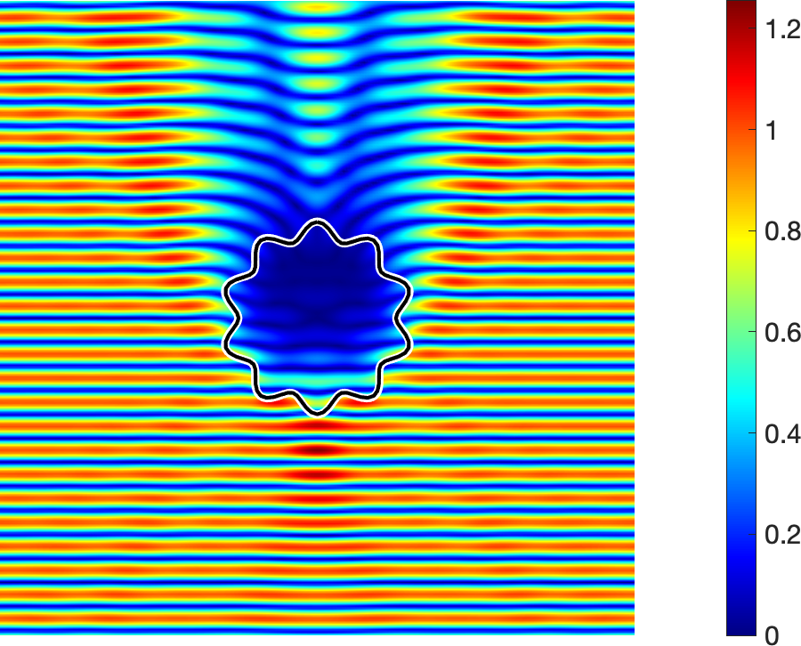
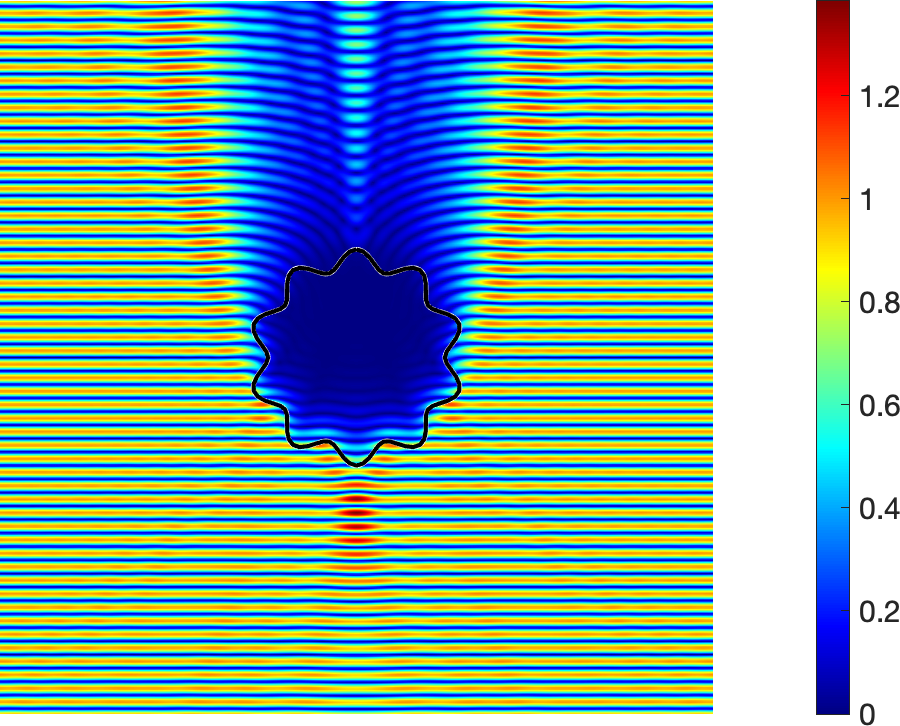
Figure 8: Visualization of the interior and exterior total electric fields $|\mathop{\mathrm{Re}}\boldsymbol{E}_{\mathrm{tot},n}|$ induced by a H-polarized plane wave striking a Chebyshev particle with refractive index $\nu={1.0925+0.248i}$ and electromagnetic size $s={4}$ (left) and $s={8}$ (right) computed with $n={60}$ and $n={80}$ respectively.

This particle is visualized in Figure 8. In our experiments we use dielectric bodies with real refractive index $\nu=1.584$, which is the refractive index of polycarbonate, and based on numerical results in [18], absorbing bodies with complex refractive indices $\nu=1.5+0.02i,\ 1.0925+0.248i$. Thus we demonstrate our algorithm for non-absorbing, weakly-absorbing and strongly-absorbing particles. The electromagnetic size of the particles is $s=d/\lambda$ where $d$ denotes the diameter of the particle, and the commonly used size parameter is therefore $x=\pi s$.

To simplify the exposition, except where otherwise stated, we compute the near field $\boldsymbol{E}$ and the far field $\boldsymbol{E}^{\infty}_{n}$ in the $xz$-plane for incident waves with direction $\boldsymbol{d}=(0,0,1)^{T}$. Thus the scattering plane is the $xz$-plane and, following [4, Page 245], [2, Page 387], and [3, Figure 4.5, Page 204] we define V-polarization and H-polarization as being respectively perpendicular and parallel to the scattering plane. In particular, for a receiver in the $xz$-plane in the direction $\widehat{\boldsymbol{x}}=(\sin\theta,0,\cos\theta)^{T}$, we define the vertical and horizontal polarization directions respectively to be $\boldsymbol{e}_{V}=\boldsymbol{e}_{\phi}=(0,1,0)^{T}$ and $\boldsymbol{e}_{H}=\boldsymbol{e}_{\theta}=(\cos\theta,0,-\sin\theta)^{T}$. The radar cross section of the scatterer, measured in the scattering plane, is then

$$\sigma_{\mathrm{X}\mathrm{X}}(\theta)=10\log_{10}4\pi|\boldsymbol{e}_{\mathrm{X}}(\theta)\cdot\boldsymbol{E}_{\infty}(\theta)|^{2},$$ (88)

where $\mathrm{X}=\mathrm{H}$ or $\mathrm{X}=\mathrm{V}$ denotes the receiver polarization, and the incident wave polarization is chosen (H or V) to match the receiver polarization. The scattering plane and polarization are visualized in Figure 1.

Figure 1: Schematic showing vertical (V) and horizontal (H) polarization with respect to the scattering plane for an incident wave with direction $\boldsymbol{d}$ and a receiver in the direction $\widehat{\boldsymbol{x}}(\theta)$.

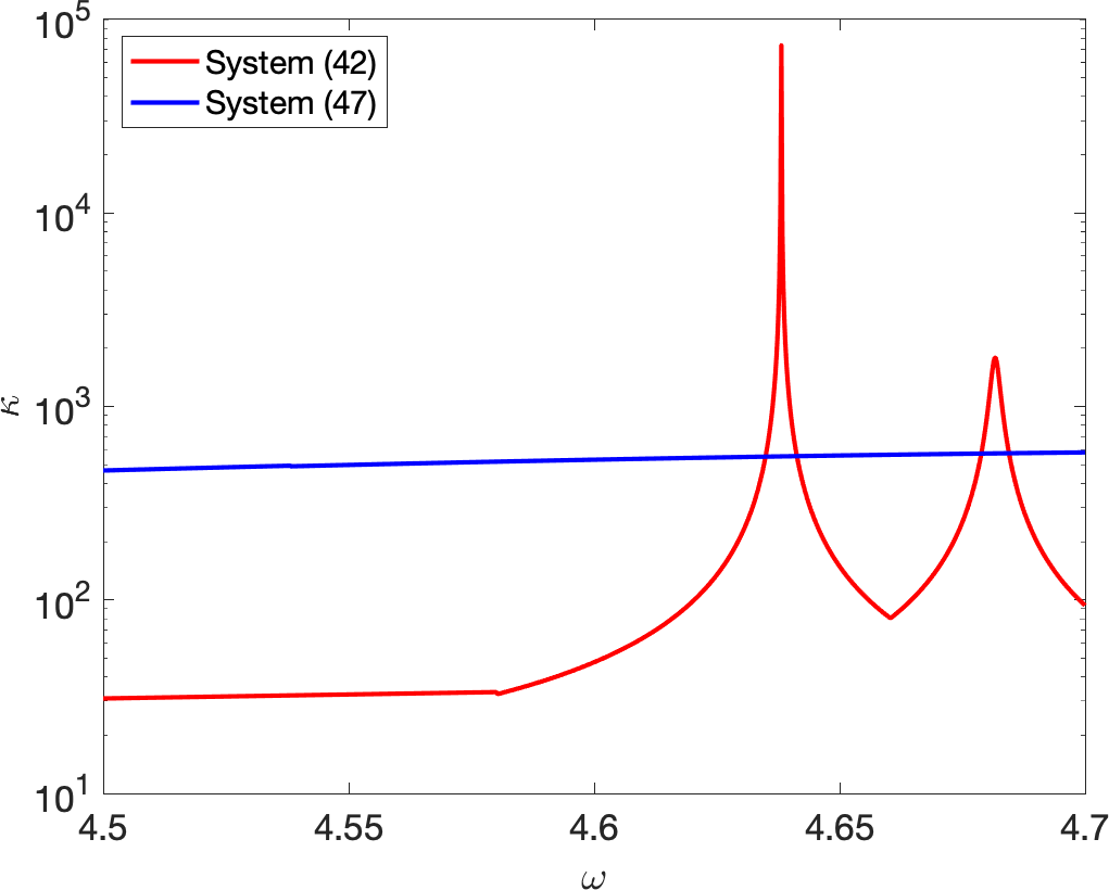
Figure 2: Condition number $\kappa$ of the matrix in systems (42) (without stabilization) and (47) (with stabilization) for a dielectric unit sphere with refractive index $\nu=1.303324617806156$ and frequency $\omega$.

In corroboration of the robust mathematical analysis in Section 4 and the appendix proving all-frequency stability and well-posedness of the continuous system, we begin by numerically demonstrating the effectiveness of the fully-discrete counterpart of our new formulation (47), governed by second-kind self-adjoint operator $I+\widetilde{\boldsymbol{\mathbb{M}}}$, compared with the related system (42), governed by $I+\boldsymbol{\mathbb{M}}$ (both without further external constraints). To this end, in Figure 2 we plot the 1-norm condition number of the matrices representing both operators (obtained using the fully-discrete representation described above) for a unit sphere dielectric scatterer with refractive index $\nu=1.303324617806156$, (for which $I+\boldsymbol{\mathbb{M}}$ has an eigenfrequency $\omega=4.638138138138138$). The plot was obtained using $1000$ frequencies $\omega$, which involves solving the Maxwell equations (4) more than $1000$ times (with fixed dielectric constants and varying incident wave frequencies). The condition number is estimated in both cases using [higham].

To demonstrate the correctness of our fully-discrete algorithm for the all-frequency stable system (47), in Tables 1–2 we tabulate the relative error

$$\mathrm{ERR}_{\mathrm{Mie},n}=\frac{\|\boldsymbol{E}_{\infty,n}(\theta)-\boldsymbol{E}_{\infty,\mathrm{ref}}(\theta)\|_{\infty}}{\|\boldsymbol{E}_{\infty,\mathrm{ref}}(\theta)\|_{\infty}}$$ (89)

for scattering of H-polarized incident plane waves by the unit sphere. The reference solution $\boldsymbol{E}_{\infty,\mathrm{ref}}$ is computed to high precision using Wiscombe’s Mie series code [22]. In practice, the maximum norms in (89) are approximated discretely using more than 1200 evenly spaced points $\theta\in[0,2\pi]$.

For nonspherical scatterers we demonstrate the correctness of our algorithm using the reciprocity relation [6, Theorem 6.30]. In particular, in Tables 3–7 we tabulate the relative error

$$\mathrm{ERR}_{\mathrm{RP},n}=\frac{\|\boldsymbol{e}_{H}(\theta)\cdot\boldsymbol{E}_{\infty,n}(\theta;\theta^{\prime})-\boldsymbol{e}_{H}(\theta^{\prime})\cdot\boldsymbol{E}_{\infty,n}(\theta^{\prime};\theta)\|_{\infty}}{\|(\boldsymbol{E}_{\infty,n}(\theta;\theta^{\prime})\cdot\boldsymbol{E}_{\infty,n}(\theta^{\prime};\theta))^{1/2}\|_{\infty}},$$ (90)

which measures the residual in the reciprocity relation. In (90) we denote by $\boldsymbol{E}_{\infty,n}(\cdot;\theta^{\prime})$ the far field induced by the $H$-polarized incident wave with direction $\boldsymbol{d}=-(\sin\theta^{\prime},0,\cos\theta^{\prime})^{T}$. The norms in (90) are over $(\theta,\theta^{\prime})\in[0,2\pi]\times[0,2\pi]$ and are approximated discretely using more than $1200\times 1200$ points. The tabulated results demonstrate the superalgebraic convergence esablished by the numerical analysis in (58). In particular, high order accuracy is attained with only a small increase in the discretization parameter $n$ (with $r$ in (58) sufficiently large due to smoothness of the test particles). In Table 8 we tabulate the CPU time and memory for computing the non-convex penetrable Chebyshev particle results in Tables 5–7, demonstrating that the spectral accuracy of our fully-discrete algorithm facilitates simulation of the low to medium-frequency Maxwell model in three dimensions to high-accuracy even using laptops with multicore processors (adjusting our results, which were obtained using a decade-old Intel Xeon (E5-2670 v2) machine, to contemporary CPU architectures).

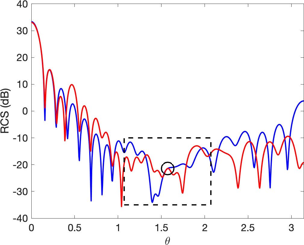
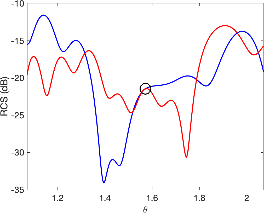
Figure 5: Visualization of the radar cross section (HH-polarization) computed with $n={80}$ of a Chebyshev particle with refractive index $\nu={1.0925+0.248i}$ and electromagnetic size $s={8}$ in original orientation (blue) and $\pi/2$-rotated orientation (red). Coincidence of the curves at $\theta=\pi/2$ is marked by a $\circ$. The right figure shows a close-up of the region indicated by the box in the left figure.

For convenient visualization of the reciprocity relation, in Figures 3–5 we plot the radar cross section $\sigma_{\mathrm{H}\mathrm{H}}$ of the Chebyshev particle in its original orientation, and rotated by an angle $\pi/2$ clockwise about the $y$-axis. The coincidence of the radar cross sections at $\theta=\pi/2$ demonstrates that the computed solutions satisfy the reciprocity relation (using the symmetry of the Chebyshev particle about the $xy$-plane).

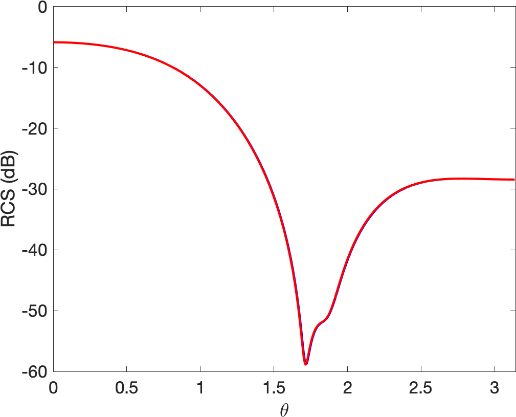
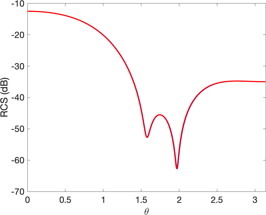
Figure 7: Visualisation of the radar cross section (HH-polarisation) computed with $n={30}$ of a spheroid with aspect ratio 5, refractive index $\nu={1.584}$ (left) and $\nu={1.0925+0.248i}$ (right), and electromagnetic size $s={1}$ computed using this algorithm (blue) and Mishchenko’s code (red).

In Figure 6 we demonstrate the visual agreement of the radar cross section $\sigma_{\mathrm{H}\mathrm{H}}$ computed using our code and using Mishchenko’s null-field-method code (downloaded from [23] and documented in [24]) for spheroids with aspect ratio $\rho=2$ and electromagnetic size $s=8$. In Figure 7 we demonstrate similar agreement for spheroids with aspect ratio $\rho=5$ and electromagnetic size $s=1$. The null field method is not able to compute the radar cross section for spheroids with such large aspect ratio $\rho=5$ and electromagnetic size $s=8$ because it exhibits numerical instability for large aspect ratio scatterers and large electromagnetic sizes [18]. The target accuracy of the computations using Mishchenko’s code is about $10^{-3}$.

Finally, in Figure 8 we visualize the total field $|\mathop{\mathrm{Re}}\boldsymbol{E}_{\mathrm{tot},n}(\boldsymbol{x})|$ for Chebyshev particles with electromagnetic size $s=1$ and $s=8$ illuminated by an H-polarized incident plane wave.

	$\nu=1.584$	$\nu=1.5+0.02i$	$\nu=1.0925+0.248i$
$n$	$\mathrm{ERR}_{\mathrm{Mie},n}$	$\mathrm{ERR}_{\mathrm{Mie},n}$	$\mathrm{ERR}_{\mathrm{Mie},n}$
5	8.04e-03	7.35e-03	6.72e-03
10	1.25e-09	1.17e-09	1.26e-09
15	1.03e-09	1.02e-09	1.61e-09

Table 1: Scattering by a sphere with diameter $\lambda$.

	$\nu=1.584$	$\nu=1.5+0.02i$	$\nu=1.0925+0.248i$
$n$	$\mathrm{ERR}_{\mathrm{Mie},n}$	$\mathrm{ERR}_{\mathrm{Mie},n}$	$\mathrm{ERR}_{\mathrm{Mie},n}$
30	1.46e-01	1.27e-01	5.79e-04
35	1.91e-03	1.59e-04	3.15e-07
40	1.98e-08	2.18e-10	5.65e-11

Table 2: Scattering by a sphere with diameter $8\lambda$.

	$\nu=1.584$	$\nu=1.5+0.02i$	$\nu=1.0925+0.248i$
$n$	$\mathrm{ERR}_{\mathrm{RP},n}$	$\mathrm{ERR}_{\mathrm{RP},n}$	$\mathrm{ERR}_{\mathrm{RP},n}$
Aspect ratio 2
5	1.61e-03	1.44e-03	1.52e-03
10	3.76e-07	3.37e-07	6.31e-07
15	1.39e-09	1.30e-09	1.45e-09
Aspect ratio 3
5	1.61e-03	1.27e-03	1.74e-03
15	2.84e-07	2.87e-07	3.66e-07
25	1.52e-10	1.54e-10	1.97e-10
Aspect ratio 4
5	2.00e-03	1.64e-03	2.72e-03
15	2.95e-06	3.14e-06	4.81e-06
25	9.49e-09	1.01e-08	1.55e-08
Aspect ratio 5
10	9.93e-05	1.33e-04	5.27e-04
20	5.23e-07	7.24e-07	3.32e-06
30	4.16e-09	6.03e-09	3.21e-08

Table 3: Scattering by a spheroid with diameter $\lambda$.

	$\nu=1.584$	$\nu=1.5+0.02i$	$\nu=1.0925+0.248i$
$n$	$\mathrm{ERR}_{\mathrm{RP},n}$	$\mathrm{ERR}_{\mathrm{RP},n}$	$\mathrm{ERR}_{\mathrm{RP},n}$
Aspect ratio 2
20	4.62e-01	3.77e-01	7.99e-01
30	6.33e-02	1.76e-02	8.53e-04
40	9.33e-05	4.36e-07	8.48e-12
Aspect ratio 3
20	2.80e-01	3.93e-01	5.73e-01
30	4.72e-02	2.64e-02	1.23e-03
40	9.37e-05	1.76e-06	2.71e-11
Aspect ratio 4
20	3.82e-01	2.47e-01	4.46e-01
30	7.78e-02	2.88e-02	1.00e-03
40	1.36e-04	3.52e-06	1.02e-10
Aspect ratio 5
20	2.11e-01	1.95e-01	4.11e-01
30	4.23e-02	3.07e-02	6.80e-04
40	1.45e-04	1.91e-06	2.05e-09

Table 4: Scattering by a spheroid with diameter $8\lambda$.

	$\nu=1.584$	$\nu=1.5+0.02i$	$\nu=1.0925+0.248i$
$n$	$\mathrm{ERR}_{\mathrm{RP},n}$	$\mathrm{ERR}_{\mathrm{RP},n}$	$\mathrm{ERR}_{\mathrm{RP},n}$
20	9.36e-03	9.26e-03	1.25e-02
30	5.21e-04	6.04e-04	1.23e-03
40	1.03e-04	9.92e-05	1.24e-04

Table 5: Scattering by a Chebyshev particle with diameter $\lambda$.

	$\nu=1.584$	$\nu=1.5+0.02i$	$\nu=1.0925+0.248i$
$n$	$\mathrm{ERR}_{\mathrm{RP},n}$	$\mathrm{ERR}_{\mathrm{RP},n}$	$\mathrm{ERR}_{\mathrm{RP},n}$
40	1.64e-03	8.77e-04	2.00e-04
50	7.49e-05	5.15e-05	2.48e-05
60	1.02e-05	6.00e-06	4.01e-06

Table 6: Scattering by a Chebyshev particle with diameter $4\lambda$.

	$\nu=1.584$	$\nu=1.5+0.02i$	$\nu=1.0925+0.248i$
$n$	$\mathrm{ERR}_{\mathrm{RP},n}$	$\mathrm{ERR}_{\mathrm{RP},n}$	$\mathrm{ERR}_{\mathrm{RP},n}$
60	7.89e-03	1.19e-03	1.26e-02
70	4.39e-04	8.74e-05	4.96e-04
80	2.69e-05	5.16e-06	2.09e-05

Table 7: Scattering by a Chebyshev particle with diameter $8\lambda$.

$n$	memory	CPU time
20	107 MB	2.4 min
40	1.52 GB	20.2 min
60	7.43 GB	1.9 h
80	23.09 GB	8.8 h

Table 8: Memory required to store the discretization matrix and CPU walltime for computing the far-field for 1202 distinct incident plane waves for the non-convex Chebyshev particles (with high-order accuracy indicated in Tables 5–7). CPU times are in parallel on a single compute node with two 10-core 2.5 GHz Intel Xeon (E5-2670 v2) processors (introduced in 2013).

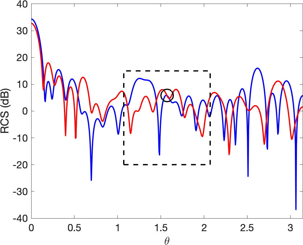
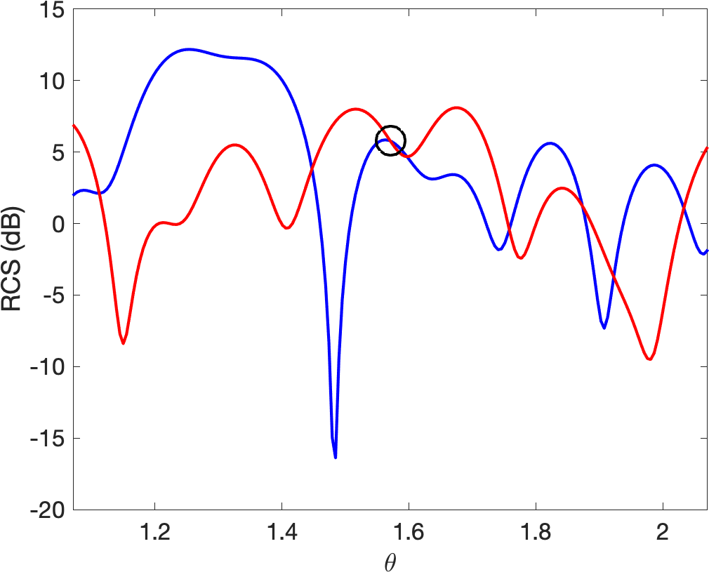
Figure 3: Visualization of the radar cross section (HH-polarization) computed with $n={80}$ of a Chebyshev particle with refractive index $\nu={1.584}$ and electromagnetic size $s={8}$ in original orientation (blue) and $\pi/2$-rotated orientation (red). Coincidence of the curves at $\theta=\pi/2$ is marked by a $\circ$. The right figure shows a close-up of the region indicated by the box in the left figure.

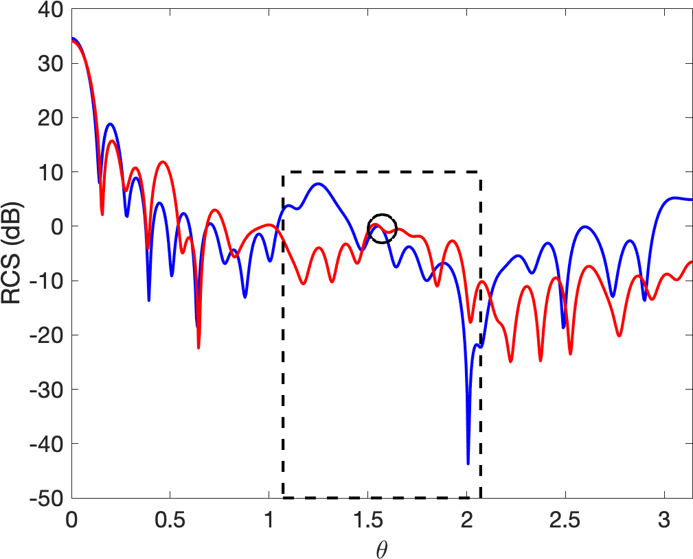
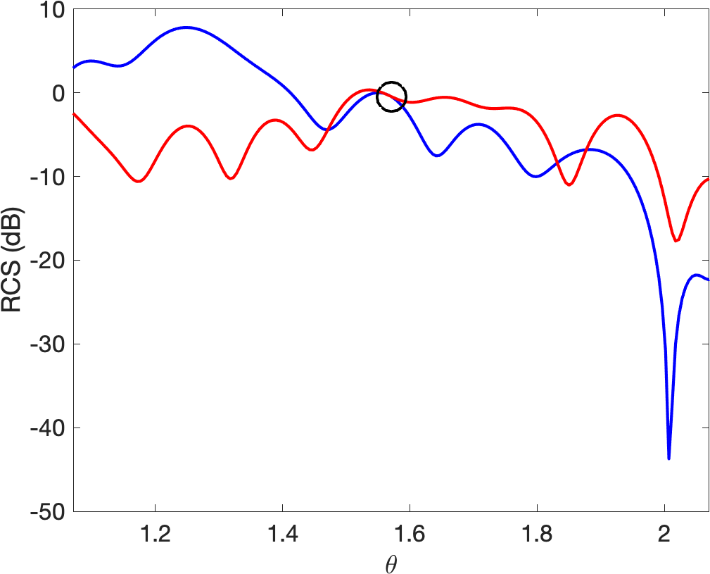
Figure 4: Visualization of the radar cross section (HH-polarization) computed with $n={80}$ of a Chebyshev particle with refractive index $\nu={1.5+0.02i}$ and electromagnetic size $s={8}$ in original orientation (blue) and $\pi/2$-rotated orientation (red). Coincidence of the curves at $\theta=\pi/2$ is marked by a $\circ$. The right figure shows a close-up of the region indicated by the box in the left figure.

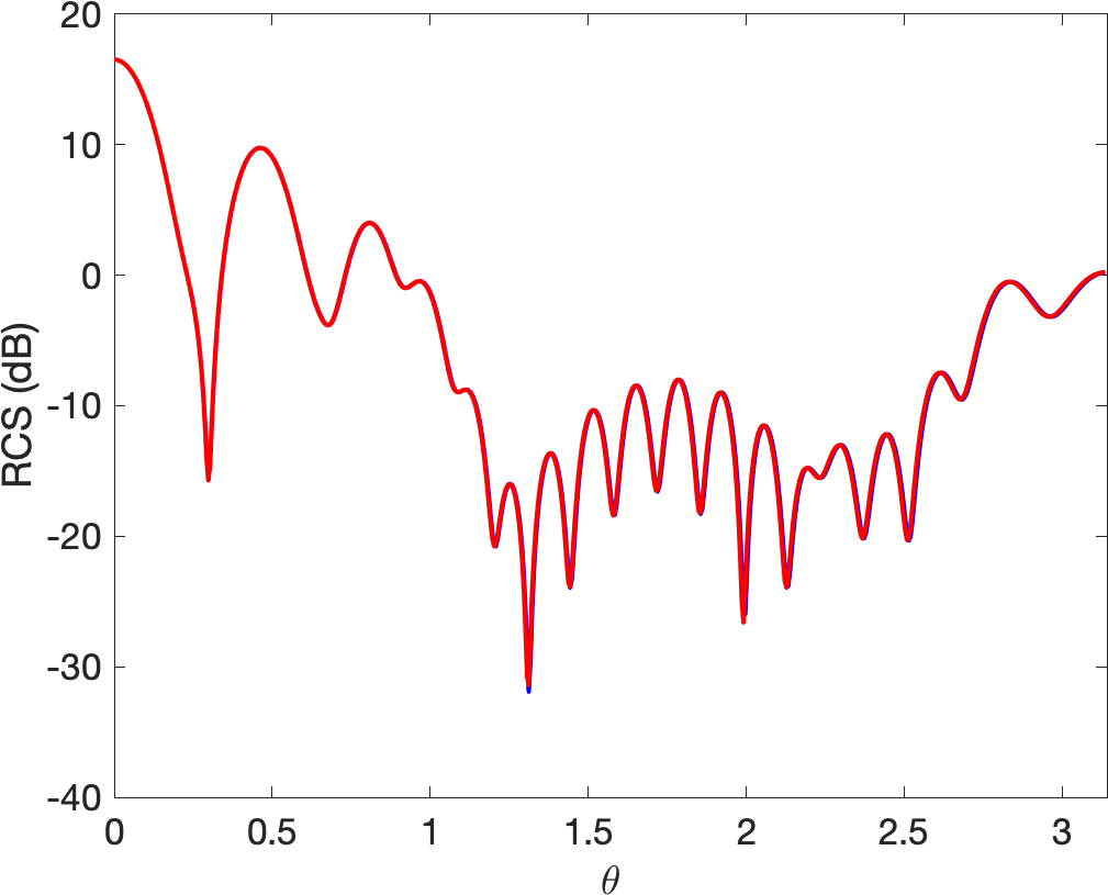
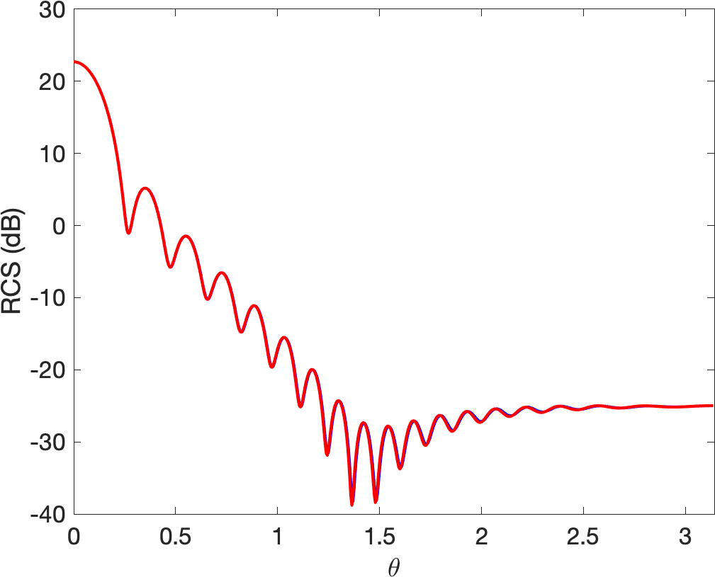
Figure 6: Visualisation of the radar cross section (HH-polarisation) computed with $n={50}$ of a spheroid with aspect ratio 2, refractive index $\nu={1.584}$ (left) and $\nu={1.0925+0.248i}$ (right), and electromagnetic size $s={8}$ computed using this algorithm (blue) and Mishchenko’s code (red).

Appendix A Singularity of standard coupling approach

Proposition A.1.

Let $H$ be a Hilbert space. Assume that either $H$ is finite dimensional with $\dim H\geq 2$ or $H$ is separable. There exist two compact linear operators $\boldsymbol{\mathbb{M}},\boldsymbol{\mathbb{J}}:H\rightarrow H$ such that $N(\boldsymbol{\mathbb{J}})\cap N(\boldsymbol{\mathbb{I}}+\boldsymbol{\mathbb{M}})=\{0\}$ and, for every $\xi\in\mathbb{C}$, $\boldsymbol{\mathbb{I}}+\boldsymbol{\mathbb{M}}+\xi\boldsymbol{\mathbb{J}}$ is singular.

Proof.

In dimension 2 we set

$$\boldsymbol{\mathbb{I}}+\boldsymbol{\mathbb{M}}=\left(\begin{array}[]{cc}1&0\\ 0&0\end{array}\right),\quad\boldsymbol{\mathbb{J}}=\left(\begin{array}[]{cc}0&1\\ 0&0\end{array}\right)$$

It is clear that $\boldsymbol{\mathbb{I}}+\boldsymbol{\mathbb{M}}+\xi\boldsymbol{\mathbb{J}}$ is singular, for any $\xi\in\mathbb{C}$. Generalizing this example to higher dimensions is trivial using block matrices.

Let $H$ be a separable Hilbert space and $\{e_{i}:i\in\mathbb{N},i\geq 1\}$ a Hilbert basis of $H$. Define $\boldsymbol{\mathbb{M}}$ by

$$\boldsymbol{\mathbb{M}}e_{i}=\left\{\begin{array}[]{lll}-e_{i},&&\mbox{for $i=2$},\\ 0,&&\mbox{for $i\neq 2$,}\end{array}\right.$$

and $\boldsymbol{\mathbb{J}}$ by

$$\boldsymbol{\mathbb{J}}e_{i}=\left\{\begin{array}[]{lll}e_{1},&&\mbox{for $i=2$},\\ 0,&&\mbox{for $i\neq 2$.}\end{array}\right.$$

A simple calculation can show that $N(\boldsymbol{\mathbb{J}})\cap N(\boldsymbol{\mathbb{I}}+\boldsymbol{\mathbb{M}})=\{0\}$ and $(\boldsymbol{\mathbb{I}}+\boldsymbol{\mathbb{M}}+\xi\boldsymbol{\mathbb{J}})(\xi e_{1}-e_{2})=0$ for any $\xi\in\mathbb{C}$. ∎

Remark 8.

In dimension three or higher, or in a separable Hilbert space, $\boldsymbol{\mathbb{I}}+\boldsymbol{\mathbb{M}}+\xi\boldsymbol{\mathbb{J}}$ may be singular for all $\xi\in\mathbb{C}$, even if both $\boldsymbol{\mathbb{M}}$ and $\boldsymbol{\mathbb{J}}$ are symmetric, compact, and $N(\boldsymbol{\mathbb{J}})\cap N(\boldsymbol{\mathbb{I}}+\boldsymbol{\mathbb{M}})=\{0\}$. In dimension 3, set

$$\boldsymbol{\mathbb{I}}+\boldsymbol{\mathbb{M}}=\left(\begin{array}[]{ccc}0&0&1\\ 0&0&1\\ 1&1&0\end{array}\right),\quad\boldsymbol{\mathbb{J}}=\left(\begin{array}[]{ccc}1&0&0\\ 0&-1&0\\ 0&0&0\end{array}\right).$$

We note that $N(\boldsymbol{\mathbb{J}})\cap N(\boldsymbol{\mathbb{I}}+\boldsymbol{\mathbb{M}})=\{0\}$ and yet $(\boldsymbol{\mathbb{I}}+\boldsymbol{\mathbb{M}}+\xi\boldsymbol{\mathbb{J}})(1,-1,-\xi)=0$, for all $\xi\in\mathbb{C}$. This counterexample can be easily extended to any separable Hilbert space.

In contrast, with the additional assumption that $\boldsymbol{\mathbb{J}}$ is non-negative, we have the following result.

Theorem 9.

Let $H$ be a Hilbert space and $\boldsymbol{\mathbb{M}},\boldsymbol{\mathbb{J}}:H\rightarrow H$ two self adjoint linear operators such that $N(\boldsymbol{\mathbb{J}})\cap N(\boldsymbol{\mathbb{I}}+\boldsymbol{\mathbb{M}})=\{0\}$. Assume that $\boldsymbol{\mathbb{J}}$ is non-negative, that is, for all $x\in H$, $\langle x,\boldsymbol{\mathbb{J}}x\rangle$ is real and $\langle x,\boldsymbol{\mathbb{J}}x\rangle\geq 0$.
Then

1. If $H$ is finite dimensional dimensional, then $\boldsymbol{\mathbb{I}}+\boldsymbol{\mathbb{M}}+\xi\boldsymbol{\mathbb{J}}$ is singular for at most finitely many values of $\xi$.

2. If $H$ is a separable Hilbert space then, making the additional assumption that $\boldsymbol{\mathbb{M}}$ and $\boldsymbol{\mathbb{J}}$ are compact, $\boldsymbol{\mathbb{I}}+\boldsymbol{\mathbb{M}}+\xi\boldsymbol{\mathbb{J}}$ is invertible for all real $\xi>\xi_{0}$ where $\xi_{0}$ is some constant.

Proof.

We first examine the case where $H$ is finite dimensional and write $n=\dim H$. Let $e_{1},...,e_{p}$ be an orthogonal basis of $R(\boldsymbol{\mathbb{J}})$, and $e_{p+1}^{\prime},...,e_{n}^{\prime}$ an orthogonal basis of $N(\boldsymbol{\mathbb{J}})$. Let $P$ be the orthogonal projection on $N(\boldsymbol{\mathbb{J}})$. We note that $P(\boldsymbol{\mathbb{I}}+\boldsymbol{\mathbb{M}})P$ is a self adjoint linear operator, therefore we can find an orthogonal basis $e_{p+1},...,e_{n}$ of $N(\boldsymbol{\mathbb{J}})$ such that the matrix of $\boldsymbol{\mathbb{I}}+\boldsymbol{\mathbb{M}}+\xi\boldsymbol{\mathbb{J}}$ in the basis $e_{1},...,e_{n}$ has the following block form,

$$\left(\begin{array}[]{ccc}\boldsymbol{\mathbb{I}}_{1}+\xi\boldsymbol{\mathbb{J}}_{1,1}+\boldsymbol{\mathbb{M}}_{1,1}&\boldsymbol{\mathbb{M}}_{1,2}&\boldsymbol{\mathbb{M}}_{1,3}\\ \overline{\boldsymbol{\mathbb{M}}_{1,2}}^{T}&\boldsymbol{\mathbb{I}}_{2}+\boldsymbol{\mathbb{M}}_{2,2}&0\\ \overline{\boldsymbol{\mathbb{M}}_{1,3}}^{T}&0&0\end{array}\right),$$ (91)

where by construction, the block $\boldsymbol{\mathbb{I}}_{2}+\boldsymbol{\mathbb{M}}_{2,2}$ is square and invertible. From the assumption $N(\boldsymbol{\mathbb{J}})\cap N(\boldsymbol{\mathbb{I}}+\boldsymbol{\mathbb{M}})=\{0\}$, the block $\boldsymbol{\mathbb{M}}_{1,3}$ is injective. Now assume that $(\boldsymbol{\mathbb{I}}+\boldsymbol{\mathbb{M}}+\xi\boldsymbol{\mathbb{J}})x=0$, and write $x$ in the block form $(x_{1},x_{2},x_{3})$. We first note that

$$\overline{\boldsymbol{\mathbb{M}}_{1,3}}^{T}x_{1}=0.$$ (92)

Next, using the second row of the block matrix in (91) and the fact that $\boldsymbol{\mathbb{I}}_{2}+\boldsymbol{\mathbb{M}}_{2,2}$ is square and invertible, we write,

$$x_{2}=-(\boldsymbol{\mathbb{I}}_{2}+\boldsymbol{\mathbb{M}}_{2,2})^{-1}\overline{\boldsymbol{\mathbb{M}}_{1,2}}^{T}x_{1}.$$ (93)

Then we have $(\boldsymbol{\mathbb{I}}_{1}+\xi\boldsymbol{\mathbb{J}}_{1,1}+\boldsymbol{\mathbb{M}}_{1,1})x_{1}+\boldsymbol{\mathbb{M}}_{1,2}x_{2}+\boldsymbol{\mathbb{M}}_{1,3}x_{3}=0$, and left multiplying by $\overline{x_{1}}^{T}$, using (92) and (93), we find

$$\overline{x_{1}}^{T}(\boldsymbol{\mathbb{I}}_{1}+\xi\boldsymbol{\mathbb{J}}_{1,1}+\boldsymbol{\mathbb{M}}_{1,1}-\boldsymbol{\mathbb{M}}_{1,2}(\boldsymbol{\mathbb{I}}_{2}+\boldsymbol{\mathbb{M}}_{2,2})^{-1}\overline{\boldsymbol{\mathbb{M}}_{1,2}}^{T})x_{1}=0.$$ (94)

Since the block $\boldsymbol{\mathbb{J}}_{1,1}$ is self adjoint and strictly positive, there is a $\xi_{0}>0$ such that for all $\xi>\xi_{0}$, the block $(\boldsymbol{\mathbb{I}}_{1}+\xi\boldsymbol{\mathbb{J}}_{1,1}+\boldsymbol{\mathbb{M}}_{1,1}-\boldsymbol{\mathbb{M}}_{1,2}(\boldsymbol{\mathbb{I}}_{2}+\boldsymbol{\mathbb{M}}_{2,2})^{-1}\overline{\boldsymbol{\mathbb{M}}_{1,2}}^{T})$ is strictly positive. Thus for $\xi>\xi_{0}$, we have that $x_{1}=0$. From (93), it follows that $x_{2}=0$. Since the block $\boldsymbol{\mathbb{M}}_{1,3}$ is injective, we infer that $x_{3}=0$. We have now proved that $\boldsymbol{\mathbb{I}}+\boldsymbol{\mathbb{M}}+\xi\boldsymbol{\mathbb{J}}$ is regular for all $\xi>\xi_{0}$. We know that $\det(\boldsymbol{\mathbb{I}}+\boldsymbol{\mathbb{M}}+\xi\boldsymbol{\mathbb{J}})$ is a polynomial in $\xi$ with degree less or equal than $n$. We have proved that it is not the zero polynomial: it thus has at most $n$ roots. For any $\xi$ different from those roots, $\boldsymbol{\mathbb{I}}+\boldsymbol{\mathbb{M}}+\xi\boldsymbol{\mathbb{J}}$ is regular. ∎

To generalize this proof to infinite dimensional spaces, we will need the following lemma.

Lemma 10.

Let $H$ be a Hilbert space, $K:H\rightarrow H$ a compact linear operator, and $\{e_{1},...,e_{n},..\}$ an orthonormal set of $H$. Then $\lim_{n\rightarrow\infty}Ke_{n}=0$.

Proof.

Arguing by contradiction, suppose that $Ke_{n}$ does not converge to zero. Then there is a positive $\epsilon$ and a subsequence $(e_{n_{j}})$ such that $\|Ke_{n_{j}}\|\geq\epsilon$ for all $j\in\mathbb{N}$. As $K$ is compact, the sequence $(Ke_{n_{j}})$ has a convergent subsequence: for ease of notation, we still denote it by $Ke_{n_{j}}$. Denote by $v$ the limit of $Ke_{n_{j}}$. Then

$$\lim_{j\rightarrow\infty}\langle v,Ke_{n_{j}}\rangle=\|v\|^{2}\geq\epsilon^{2}.$$

But $\langle v,Ke_{n_{j}}\rangle=\langle K^{*}v,e_{n_{j}}\rangle$ and

$$\|K^{*}v\|^{2}\geq\sum_{n=1}^{\infty}|\langle K^{*}v,e_{n}\rangle|^{2}.$$

This is a contradiction.

Let us now denote by $P_{1}$ the orthogonal projection on $N(\boldsymbol{\mathbb{J}})^{\perp}$. Since $\boldsymbol{\mathbb{M}}$ is compact, the range $R((\boldsymbol{\mathbb{I}}-P_{1})(\boldsymbol{\mathbb{I}}+\boldsymbol{\mathbb{M}})(\boldsymbol{\mathbb{I}}-P_{1}))$ is closed: let $P_{2}$ be the orthogonal projection on that range. We observe that $P_{1}P_{2}=0$, and since $P_{1}$ and $P_{2}$ are both self adjoint, $P_{2}P_{1}=0$. It follows that $P_{1}+P_{2}$ is also an orthogonal projector. Set $P_{3}=\boldsymbol{\mathbb{I}}-P_{1}-P_{2}$. The following properties hold:

$$\forall x\in H,\quad x=P_{1}x+P_{2}x+P_{3}x,$$ (95)

$$\forall x\in H,\quad\|x\|^{2}=\|P_{1}x\|^{2}+\|P_{2}x\|^{2}+\|P_{3}x\|^{2},$$ (96)

$$P_{i}P_{j}=\delta_{ij}P_{i},\quad\forall i,j\in\{1,2,3\}.$$ (97)

Next, we write

$$\boldsymbol{\mathbb{I}}+\boldsymbol{\mathbb{M}}+\xi\boldsymbol{\mathbb{J}}= P_{1}(\boldsymbol{\mathbb{I}}+\boldsymbol{\mathbb{M}}+\xi\boldsymbol{\mathbb{J}})P_{1} + P_{1}(\boldsymbol{\mathbb{I}}+\boldsymbol{\mathbb{M}})P_{2} + P_{1}(\boldsymbol{\mathbb{I}}+\boldsymbol{\mathbb{M}})P_{3}$$

$$\ {}+P_{2}(\boldsymbol{\mathbb{I}}+\boldsymbol{\mathbb{M}})P_{1} + P_{2}(\boldsymbol{\mathbb{I}}+\boldsymbol{\mathbb{M}})P_{2} + P_{2}(\boldsymbol{\mathbb{I}}+\boldsymbol{\mathbb{M}})P_{3}$$

$$\ {}+P_{3}(\boldsymbol{\mathbb{I}}+\boldsymbol{\mathbb{M}})P_{1} + P_{3}(\boldsymbol{\mathbb{I}}+\boldsymbol{\mathbb{M}})P_{2} + P_{3}(\boldsymbol{\mathbb{I}}+\boldsymbol{\mathbb{M}})P_{3}.$$ (98)

Now, $P_{1}+P_{2}$ is the orthogonal projection on the orthogonal direct sum
$N(J)^{\perp}\oplus R((\boldsymbol{\mathbb{I}}-P_{1})(\boldsymbol{\mathbb{I}}+\boldsymbol{\mathbb{M}})(\boldsymbol{\mathbb{I}}-P_{1}))$. Recall the identity $(V_{1}+V_{2})^{\perp}=V_{1}^{\perp}\cap V_{2}^{\perp}$ for any two subspaces $V_{1}$ and $V_{2}$. As $\boldsymbol{\mathbb{M}}$ and $P_{1}$ are self-adjoint, $R((\boldsymbol{\mathbb{I}}-P_{1})(\boldsymbol{\mathbb{I}}+\boldsymbol{\mathbb{M}})(\boldsymbol{\mathbb{I}}-P_{1}))^{\perp}=N((\boldsymbol{\mathbb{I}}-P_{1})(\boldsymbol{\mathbb{I}}+\boldsymbol{\mathbb{M}})(\boldsymbol{\mathbb{I}}-P_{1}))$, and it follows that $P_{3}=\boldsymbol{\mathbb{I}}-P_{1}-P_{2}$ is the orthogonal projection on $N(J)\cap N((\boldsymbol{\mathbb{I}}-P_{1})(\boldsymbol{\mathbb{I}}+\boldsymbol{\mathbb{M}})(\boldsymbol{\mathbb{I}}-P_{1}))$. We then note that

$$P_{2}(\boldsymbol{\mathbb{I}}+\boldsymbol{\mathbb{M}})P_{3}=P_{2}(\boldsymbol{\mathbb{I}}-P_{1})(\boldsymbol{\mathbb{I}}+\boldsymbol{\mathbb{M}})(\boldsymbol{\mathbb{I}}-P_{1})P_{3}=0.$$ (99)

Similarly, $P_{3}(\boldsymbol{\mathbb{I}}+\boldsymbol{\mathbb{M}})P_{3}$ is also zero. $P_{3}(\boldsymbol{\mathbb{I}}+\boldsymbol{\mathbb{M}})P_{2}$ is the adjoint of $P_{2}(\boldsymbol{\mathbb{I}}+\boldsymbol{\mathbb{M}})P_{3}$, so it is also zero. We also use (97) to simplify (98) to

$$\boldsymbol{\mathbb{I}}+\boldsymbol{\mathbb{M}}+\xi\boldsymbol{\mathbb{J}} =P_{1}(\boldsymbol{\mathbb{I}}+\boldsymbol{\mathbb{M}}+\xi\boldsymbol{\mathbb{J}})P_{1} + P_{1}\boldsymbol{\mathbb{M}}P_{2} + P_{1}\boldsymbol{\mathbb{M}}P_{3}$$

$$\quad{}+P_{2}\boldsymbol{\mathbb{M}}P_{1} + P_{2}(\boldsymbol{\mathbb{I}}+\boldsymbol{\mathbb{M}})P_{2} + 0$$

$$\quad{}+P_{3}\boldsymbol{\mathbb{M}}P_{1} + 0 + 0.$$ (100)

Next, we claim that $P_{2}(\boldsymbol{\mathbb{I}}+\boldsymbol{\mathbb{M}}):R(P_{2})\rightarrow R(P_{2})$ is a continuous and invertible operator. Indeed, as $\boldsymbol{\mathbb{M}}$ is compact, it suffices to show that if $P_{2}(\boldsymbol{\mathbb{I}}+\boldsymbol{\mathbb{M}})P_{2}y=0$, then $P_{2}y=0$. But

$$P_{2}(\boldsymbol{\mathbb{I}}+\boldsymbol{\mathbb{M}})P_{2}=(P_{2}+P_{3})(\boldsymbol{\mathbb{I}}+\boldsymbol{\mathbb{M}})(P_{2}+P_{3})=(\boldsymbol{\mathbb{I}}-P_{1})(\boldsymbol{\mathbb{I}}+\boldsymbol{\mathbb{M}})(\boldsymbol{\mathbb{I}}-P_{1}),$$

and

$$N((\boldsymbol{\mathbb{I}}-P_{1})(\boldsymbol{\mathbb{I}}+\boldsymbol{\mathbb{M}})(\boldsymbol{\mathbb{I}}-P_{1})) =\left(N(J)\cap N((\boldsymbol{\mathbb{I}}-P_{1})(\boldsymbol{\mathbb{I}}+\boldsymbol{\mathbb{M}})(\boldsymbol{\mathbb{I}}-P_{1}))\right)$$

$$\qquad{}\oplus\left(N(J)^{\perp}\cap N((\boldsymbol{\mathbb{I}}-P_{1})(\boldsymbol{\mathbb{I}}+\boldsymbol{\mathbb{M}})(\boldsymbol{\mathbb{I}}-P_{1}))\right),$$ (101)

thus

$$N((\boldsymbol{\mathbb{I}}-P_{1})(\boldsymbol{\mathbb{I}}+\boldsymbol{\mathbb{M}})(\boldsymbol{\mathbb{I}}-P_{1}))\cap R(P_{2})=\{0\},$$

so $(\boldsymbol{\mathbb{I}}-P_{1})(\boldsymbol{\mathbb{I}}+\boldsymbol{\mathbb{M}})(\boldsymbol{\mathbb{I}}-P_{1})P_{2}y=0$ implies that $P_{2}y=0$, proving the claim.
Let $Q$ be the inverse of $P_{2}(\boldsymbol{\mathbb{I}}+\boldsymbol{\mathbb{M}}):R(P_{2})\rightarrow R(P_{2})$. Assume now that $x\in H$ is such that $(\boldsymbol{\mathbb{I}}+\boldsymbol{\mathbb{M}}+\xi\boldsymbol{\mathbb{J}})x=0$. Therefore, from (100),

$$P_{2}x=-QP_{2}\boldsymbol{\mathbb{M}}P_{1}x.$$ (102)

Also from (100), since $P_{3}\boldsymbol{\mathbb{M}}P_{1}x=0$ and $\boldsymbol{\mathbb{M}}$, $P_{1}$, $P_{3}$ are self adjoint, we infer that

$$\langle P_{1}x,(\boldsymbol{\mathbb{I}}+\xi P_{1}\boldsymbol{\mathbb{J}}P_{1}+P_{1}\boldsymbol{\mathbb{M}}P_{1}-P_{1}\boldsymbol{\mathbb{M}}QP_{2}\boldsymbol{\mathbb{M}}P_{1})P_{1}x\rangle=0.$$ (103)

Henceforth, for brevity we write $A=P_{1}\boldsymbol{\mathbb{M}}P_{1}-P_{1}\boldsymbol{\mathbb{M}}QP_{2}\boldsymbol{\mathbb{M}}P_{1}$. If $R(P_{1})$ is finite dimensional, according to the argument carried out above, it is clear that for all sufficiently large $\xi$, (103) implies that $P_{1}x=0$, since $\langle y,P_{1}\boldsymbol{\mathbb{J}}P_{1}y>\geq 0$ if $y\neq>0$.

Otherwise, $R(P_{1})$ is infinite dimensional, and a more detailed argument is needed. Let $e_{1},\dots,e_{n},\dots$ be an orthonormal basis of eigenvectors for the strictly positive self adjoint operator $P_{1}\boldsymbol{\mathbb{J}}P_{1}:R(P_{1})\rightarrow R(P_{1})$. Without loss of generality, we assume that the sequence $\langle e_{n},P_{1}\boldsymbol{\mathbb{J}}P_{1}e_{n}\rangle$ is decreasing. Note that $A:R(P_{1})\rightarrow R(P_{1})$ is a compact linear operator, so according to Lemma 10, $\lim_{n\rightarrow\infty}Ae_{n}=0$. Pick $N$ such that for all $n>N$, $\|Ae_{n}\|\leq\frac{1}{4}$. Let $P_{4}$ be the orthogonal projection from $H$ to $\mathop{\mathrm{Span}}\{e_{1},...,e_{N}\}$. There is a positive $\xi_{0}$ such that for all $\xi>\xi_{0}$, and for all $y\in H$,

$$\mathop{\mathrm{Re}}\langle P_{4}y,(\boldsymbol{\mathbb{I}}+\xi P_{1}\boldsymbol{\mathbb{J}}P_{1}+A)P_{4}y\rangle\geq\frac{1}{2}\|P_{4}y\|^{2}.$$ (104)

Next, for any $y\in R(P_{1})$,

$$\mathop{\mathrm{Re}}\langle(I-P_{4})y,(\boldsymbol{\mathbb{I}}+\xi P_{1}\boldsymbol{\mathbb{J}}P_{1}+A)(I-P_{4})y\rangle\geq\frac{3}{4}\|(I-P_{4})y\|^{2},$$ (105)

and

$$\mathop{\mathrm{Re}}\langle P_{4}y,(\boldsymbol{\mathbb{I}}+\xi P_{1}\boldsymbol{\mathbb{J}}P_{1}+A)(I-P_{4})y\rangle=\mathop{\mathrm{Re}}\langle P_{4}y,A(I-P_{4})y\rangle$$

$$\geq-\frac{1}{8}\|P_{4}y\|^{2}-2\|A(I-P_{4})y\|^{2}\geq-\frac{1}{8}\|P_{4}y\|^{2}-\frac{1}{8}\|(I-P_{4})y\|^{2}.$$ (106)

We then combine (104)–(106) to write, for any $y\in R(P_{1})$, and any $\xi>\xi_{0}$,

$$\mathop{\mathrm{Re}}\langle y,(\boldsymbol{\mathbb{I}}+\xi P_{1}\boldsymbol{\mathbb{J}}P_{1}+A)y\rangle$$

$$=\mathop{\mathrm{Re}}\langle P_{4}y,(\boldsymbol{\mathbb{I}}+\xi P_{1}\boldsymbol{\mathbb{J}}P_{1}+A)P_{4}y\rangle$$

$$+\mathop{\mathrm{Re}}\langle(I-P_{4})y,(\boldsymbol{\mathbb{I}}+\xi P_{1}\boldsymbol{\mathbb{J}}P_{1}+A)(I-P_{4})y\rangle$$

$$+2\mathop{\mathrm{Re}}\langle P_{4}y,(\boldsymbol{\mathbb{I}}+\xi P_{1}\boldsymbol{\mathbb{J}}P_{1}+A)(I-P_{4})y\rangle$$

$$\geq\frac{1}{4}\|P_{4}y\|^{2}+\frac{1}{2}\|(I-P_{4})y\|^{2}.$$ (107)

Recalling (103) and the definition of $A$, we infer that for any $\xi>\xi_{0}$, $P_{1}x=0$. We now recall (102) to claim that $P_{2}x=0$. Thus $x=P_{3}x$ and it now follows according to the decomposition (98) that $(\boldsymbol{\mathbb{I}}+\boldsymbol{\mathbb{M}})x=0$, so that $x\in N(\boldsymbol{\mathbb{I}}+\boldsymbol{\mathbb{M}})\cap N(\boldsymbol{\mathbb{J}})$, thus $x$ must be zero. We have thus proved that $\boldsymbol{\mathbb{I}}+\boldsymbol{\mathbb{M}}+\xi\boldsymbol{\mathbb{J}}$ is injective for all $\xi>\xi_{0}$. Since $\boldsymbol{\mathbb{M}}$ and $\boldsymbol{\mathbb{J}}$ are compact operators, $\boldsymbol{\mathbb{I}}+\boldsymbol{\mathbb{M}}+\xi\boldsymbol{\mathbb{J}}$ is invertible for all $\xi>\xi_{0}$. ∎

Appendix B Norm estimates and proof of Theorem 2

Proposition B.1.

Let $H$ be a Hilbert space and $\boldsymbol{\mathbb{M}},\boldsymbol{\mathbb{J}}:H\rightarrow H$ two compact linear operators such that $N(\boldsymbol{\mathbb{J}})\cap N(\boldsymbol{\mathbb{I}}+\boldsymbol{\mathbb{M}})=\{0\}$. Then the linear operator $\boldsymbol{\mathbb{I}}+\boldsymbol{\mathbb{M}}^{*}\boldsymbol{\mathbb{M}}+\boldsymbol{\mathbb{M}}^{*}+\boldsymbol{\mathbb{M}}+\boldsymbol{\mathbb{J}}^{*}\boldsymbol{\mathbb{J}}$ has a bounded inverse.

Proof.

We note that $\boldsymbol{\mathbb{I}}+\boldsymbol{\mathbb{M}}^{*}\boldsymbol{\mathbb{M}}+\boldsymbol{\mathbb{M}}^{*}+\boldsymbol{\mathbb{M}}=(\boldsymbol{\mathbb{I}}+\boldsymbol{\mathbb{M}})^{*}(\boldsymbol{\mathbb{I}}+\boldsymbol{\mathbb{M}})$. If $x\in H$ is such that $(\boldsymbol{\mathbb{I}}+\boldsymbol{\mathbb{M}})^{*}(\boldsymbol{\mathbb{I}}+\boldsymbol{\mathbb{M}})x+\boldsymbol{\mathbb{J}}^{*}\boldsymbol{\mathbb{J}}x=0$, then $\|(\boldsymbol{\mathbb{I}}+\boldsymbol{\mathbb{M}})x\|^{2}+\|\boldsymbol{\mathbb{J}}x\|^{2}=0$, so $x\in N(\boldsymbol{\mathbb{J}})\cap N(\boldsymbol{\mathbb{I}}+\boldsymbol{\mathbb{M}})$. It follows that, due to our assumption, $x$ must be zero. Since $\boldsymbol{\mathbb{M}}^{*}\boldsymbol{\mathbb{M}}+\boldsymbol{\mathbb{M}}^{*}+\boldsymbol{\mathbb{M}}+\boldsymbol{\mathbb{J}}^{*}\boldsymbol{\mathbb{J}}$ is compact, it follows that $\boldsymbol{\mathbb{I}}+\boldsymbol{\mathbb{M}}^{*}\boldsymbol{\mathbb{M}}+\boldsymbol{\mathbb{M}}^{*}+\boldsymbol{\mathbb{M}}+\boldsymbol{\mathbb{J}}^{*}\boldsymbol{\mathbb{J}}$ has a bounded inverse. ∎

Proposition B.2.

Let $H,\boldsymbol{\mathbb{M}},\boldsymbol{\mathbb{J}}$ be defined as in the previous proposition, with $N(\boldsymbol{\mathbb{J}})\cap N(\boldsymbol{\mathbb{I}}+\boldsymbol{\mathbb{M}})=\{0\}$. Assume also that the system of equations

$$\left\{\begin{array}[]{l}(\boldsymbol{\mathbb{I}}+\boldsymbol{\mathbb{M}})x=b\\ \boldsymbol{\mathbb{J}}x=0\end{array}\right.$$ (108)

has a solution $x_{0}\in H$. Then $x_{0}$ is the unique solution to the equation

$$(\boldsymbol{\mathbb{I}}+\boldsymbol{\mathbb{M}}^{*}\boldsymbol{\mathbb{M}}+\boldsymbol{\mathbb{M}}^{*}+\boldsymbol{\mathbb{M}}+\boldsymbol{\mathbb{J}}^{*}\boldsymbol{\mathbb{J}})x=(\boldsymbol{\mathbb{I}}+\boldsymbol{\mathbb{M}}^{*})b.$$ (109)

Proof.

Uniqueness follows from Proposition B.1. Since $x_{0}$ satisfies (108) it is clear that $(\boldsymbol{\mathbb{I}}+\boldsymbol{\mathbb{M}}^{*})(\boldsymbol{\mathbb{I}}+\boldsymbol{\mathbb{M}})x_{0}=(\boldsymbol{\mathbb{I}}+\boldsymbol{\mathbb{M}}^{*})b$ and $\boldsymbol{\mathbb{J}}^{*}\boldsymbol{\mathbb{J}}x_{0}=0$. Thus $x_{0}$ satisfies (109). ∎

B.1 Estimating the norm of $(\boldsymbol{\mathbb{I}}+\boldsymbol{\mathbb{M}}^{*}\boldsymbol{\mathbb{M}}+\boldsymbol{\mathbb{M}}^{*}+\boldsymbol{\mathbb{M}}+\boldsymbol{\mathbb{J}}^{*}\boldsymbol{\mathbb{J}})^{-1}$

We show in this section how the norm of $(\boldsymbol{\mathbb{I}}+\boldsymbol{\mathbb{M}}^{*}\boldsymbol{\mathbb{M}}+\boldsymbol{\mathbb{M}}^{*}+\boldsymbol{\mathbb{M}}+\boldsymbol{\mathbb{J}}^{*}\boldsymbol{\mathbb{J}})^{-1}$ can be estimated using the norms of $\boldsymbol{\mathbb{M}}$ and $\boldsymbol{\mathbb{J}}$, a constant that measures "how well" $(\boldsymbol{\mathbb{I}}+\boldsymbol{\mathbb{M}})$ is invertible on the orthogonal of $N(\boldsymbol{\mathbb{I}}+\boldsymbol{\mathbb{M}})$, and using another constant that measures “how positive” $\boldsymbol{\mathbb{J}}^{*}\boldsymbol{\mathbb{J}}$ is on $N(\boldsymbol{\mathbb{I}}+\boldsymbol{\mathbb{M}})$.

We first note that $\boldsymbol{\mathbb{I}}+\boldsymbol{\mathbb{M}}$ is bijective from $N(\boldsymbol{\mathbb{I}}+\boldsymbol{\mathbb{M}})^{\perp}$ to $R(\boldsymbol{\mathbb{I}}+\boldsymbol{\mathbb{M}})$, and that its inverse is bounded. Denote by $P$ the orthogonal projection on $N(\boldsymbol{\mathbb{I}}+\boldsymbol{\mathbb{M}})$. There is a positive constant $C_{1}$ such that for all $x\in H$,

$$\|(\boldsymbol{\mathbb{I}}-P)x\|\leq C_{1}\|(\boldsymbol{\mathbb{I}}+\boldsymbol{\mathbb{M}})(\boldsymbol{\mathbb{I}}-P)x\|.$$ (110)

Next we note that $N(\boldsymbol{\mathbb{I}}+\boldsymbol{\mathbb{M}})$ is finite dimensional. Using that $N(\boldsymbol{\mathbb{J}})\cap N(\boldsymbol{\mathbb{I}}+\boldsymbol{\mathbb{M}})=\{0\}$, $\|\boldsymbol{\mathbb{J}}\|$ achieves a strictly positive minimum on the compact set $\{x:x\in N(\boldsymbol{\mathbb{I}}+\boldsymbol{\mathbb{M}}),\,\|x\|=1\}$. Therefore, there is a positive constant $C_{2}$ such that for all $x\in H$,

$$\|Px\|\leq C_{2}\|\boldsymbol{\mathbb{J}}Px\|.$$ (111)

Assume now that

$$(\boldsymbol{\mathbb{I}}+\boldsymbol{\mathbb{M}})^{*}(\boldsymbol{\mathbb{I}}+\boldsymbol{\mathbb{M}})x+\boldsymbol{\mathbb{J}}^{*}\boldsymbol{\mathbb{J}}x=d,$$ (112)

for some $d$, and estimate $x$.

There are two cases. Let us first consider the case when $d\in N(\boldsymbol{\mathbb{I}}+\boldsymbol{\mathbb{M}})^{\perp}$, that is, $d=(\boldsymbol{\mathbb{I}}-P)d$. Evaluating the dot product of $x$ with (112), we obtain

$$\|(\boldsymbol{\mathbb{I}}+\boldsymbol{\mathbb{M}})x\|^{2}+\|\boldsymbol{\mathbb{J}}x\|^{2}=\langle x,(\boldsymbol{\mathbb{I}}-P)d\rangle,$$

which we re-write as

$$\|(\boldsymbol{\mathbb{I}}+\boldsymbol{\mathbb{M}})(\boldsymbol{\mathbb{I}}-P)x\|^{2}+\|\boldsymbol{\mathbb{J}}x\|^{2}=\langle(\boldsymbol{\mathbb{I}}-P)x,d\rangle.$$

Using (110),

$$\frac{1}{C_{1}^{2}}\|(\boldsymbol{\mathbb{I}}-P)x\|^{2}+\|\boldsymbol{\mathbb{J}}x\|^{2}\leq\|(\boldsymbol{\mathbb{I}}-P)x\|\|d\|.$$

Thus, we obtain

$$\|(\boldsymbol{\mathbb{I}}-P)x\|\leq C_{1}^{2}\|d\|,\qquad\|\boldsymbol{\mathbb{J}}x\|\leq C_{1}\|d\|.$$ (113)

It now follows that,

$$\|\boldsymbol{\mathbb{J}}Px\|\leq\|\boldsymbol{\mathbb{J}}x\|+\|\boldsymbol{\mathbb{J}}(\boldsymbol{\mathbb{I}}-P)x\|\leq\left(C_{1}+C_{1}^{2}\|\boldsymbol{\mathbb{J}}\|\right)\|d\|,$$

and using (111),

$$\|Px\|\leq C_{2}\left(C_{1}+C_{1}^{2}\|\boldsymbol{\mathbb{J}}\|\right)\|d\|.$$ (114)

Thus, we obtain the bound

$$\|x\|^{2}=\|Px\|^{2}+\|(\boldsymbol{\mathbb{I}}-P)x\|^{2}\leq\left(C_{2}^{2}\left(C_{1}+C_{1}^{2}\|\boldsymbol{\mathbb{J}}\|\right)^{2}+C_{1}^{4}\right)\|d\|^{2}.$$ (115)

Let us now consider the case when $d\in N(\boldsymbol{\mathbb{I}}+\boldsymbol{\mathbb{M}})$ and estimate $\|x\|$ from (112). Using that $Pd=d$ and evaluating the inner product of equation (112) with $x$, we obtain,

$$\|(\boldsymbol{\mathbb{I}}+\boldsymbol{\mathbb{M}})(\boldsymbol{\mathbb{I}}-P)x\|^{2}+\|\boldsymbol{\mathbb{J}}x\|^{2}=\langle Px,d\rangle.$$ (116)

Next, we evaluate the inner product of equation (112) with $Px$ to obtain

$$\langle\boldsymbol{\mathbb{J}}Px,\boldsymbol{\mathbb{J}}x\rangle=\langle Px,d\rangle.$$ (117)

Combining (116) with (117) we arrive at

$$\|(\boldsymbol{\mathbb{I}}+\boldsymbol{\mathbb{M}})(\boldsymbol{\mathbb{I}}-P)x\|^{2}+\frac{1}{2}\|\boldsymbol{\mathbb{J}}x\|^{2}\leq\frac{1}{2}\|\boldsymbol{\mathbb{J}}Px\|^{2}.$$ (118)

From (116) and (110)

$$\|(\boldsymbol{\mathbb{I}}-P)x\|^{2}\leq C_{1}^{2}\langle Px,d\rangle.$$ (119)

Next, we note that, using (117),

$$\|\boldsymbol{\mathbb{J}}Px\|^{2}=\langle Px,d\rangle-\langle\boldsymbol{\mathbb{J}}Px,\boldsymbol{\mathbb{J}}(\boldsymbol{\mathbb{I}}-P)x\rangle\leq\langle Px,d\rangle+\frac{1}{2}\|\boldsymbol{\mathbb{J}}Px\|^{2}+\frac{1}{2}\|\boldsymbol{\mathbb{J}}(\boldsymbol{\mathbb{I}}-P)x\|^{2},$$

so combining (119) and (B.1),

$$\frac{1}{2}\|\boldsymbol{\mathbb{J}}Px\|^{2}\leq\left(1+\frac{1}{2}C_{1}^{2}\|\boldsymbol{\mathbb{J}}\|^{2}\right)\langle Px,d\rangle,$$ (120)

and recalling (111),

$$\|Px\|^{2}\leq C_{2}^{2}\left(2+C_{1}^{2}\|\boldsymbol{\mathbb{J}}\|^{2}\right)\langle Px,d\rangle\leq\frac{1}{2}\|Px\|^{2}+\frac{1}{2}C_{2}^{4}(2+C_{1}^{2}\|\boldsymbol{\mathbb{J}}\|^{2})^{2}\|d\|^{2},$$

thus

$$\|Px\|^{2}\leq C_{2}^{4}(2+C_{1}^{2}\|\boldsymbol{\mathbb{J}}\|^{2})^{2}\|d\|^{2}.$$ (121)

Using (119) one more time, it follows that

$$\|(\boldsymbol{\mathbb{I}}-P)x\|^{2}\leq C_{1}^{2}C_{2}^{2}(2+C_{1}^{2}\|\boldsymbol{\mathbb{J}}\|^{2})\|d\|^{2}.$$ (122)

Combining (121) and (122), it is clear that $\|x\|$ is bounded by a constant depending only on $C_{1},C_{2},$ and $\|\boldsymbol{\mathbb{J}}\|\|d\|$.

We covered two cases: if $d\in N(\boldsymbol{\mathbb{I}}+\boldsymbol{\mathbb{M}})^{\perp}$ then the estimate (115) holds, and if $d\in N(\boldsymbol{\mathbb{I}}+\boldsymbol{\mathbb{M}})$ then the estimate (121-122) holds. Since $H$ is the direct sum of $N(\boldsymbol{\mathbb{I}}+\boldsymbol{\mathbb{M}})^{\perp}$ and $N(\boldsymbol{\mathbb{I}}+\boldsymbol{\mathbb{M}})$ and equation (112) is linear, the estimate for $d\in H$ results from combining the previous two estimates.

B.2 Estimating the norm of $(\boldsymbol{\mathbb{I}}+\boldsymbol{\mathbb{M}}^{*}\boldsymbol{\mathbb{M}}+\boldsymbol{\mathbb{M}}^{*}+\boldsymbol{\mathbb{M}}+\boldsymbol{\mathbb{J}}^{*}\boldsymbol{\mathbb{J}})^{-1}$ in the trivial case where the nullspace of $\boldsymbol{\mathbb{I}}+\boldsymbol{\mathbb{M}}$ is reduced to zero

In this case $(\boldsymbol{\mathbb{I}}-P)=\boldsymbol{\mathbb{I}}$, so estimate (113) simply reduces to $\|x\|\leq C_{1}^{2}\|d\|$, that is, the norm of $(\boldsymbol{\mathbb{I}}+\boldsymbol{\mathbb{M}}^{*}\boldsymbol{\mathbb{M}}+\boldsymbol{\mathbb{M}}^{*}+\boldsymbol{\mathbb{M}}+\boldsymbol{\mathbb{J}}^{*}\boldsymbol{\mathbb{J}})^{-1}$ is bounded by $C_{1}^{2}$.

B.3 Proof of Theorem 2

The main achievement of [9] was to show that $N(\boldsymbol{\mathbb{I}}+\boldsymbol{\mathbb{M}})\cap N(\boldsymbol{\mathbb{J}})=\{0\}$, where $\boldsymbol{\mathbb{M}}$ and $\boldsymbol{\mathbb{J}}$ refer to those operators defined in Section 3. Accordingly, the outcome of the previous section is to claim that if $d\in\boldsymbol{\mathrm{L}}^{2}_{2}(\partial D)$ and $x$ is the unique solution to

$$(\boldsymbol{\mathbb{I}}+\boldsymbol{\mathbb{M}}^{*}\boldsymbol{\mathbb{M}}+\boldsymbol{\mathbb{M}}^{*}+\boldsymbol{\mathbb{M}}+\boldsymbol{\mathbb{J}}^{*}\boldsymbol{\mathbb{J}})x=d,$$ (123)

that there is a constant $C$ such that $\|x\|_{\boldsymbol{\mathrm{L}}^{2}_{2}(\partial D)}\leq C\|d\|_{\boldsymbol{\mathrm{L}}^{2}_{2}(\partial D)}$, where $C$ depends only on $\|\boldsymbol{\mathbb{M}}\|,\|\boldsymbol{\mathbb{J}}\|$ and on $C_{1}$ and $C_{2}$ defined in (110)–(111).

Suppose that $\partial D$ is smooth. If $d\in\boldsymbol{\mathrm{H}}^{1}_{2}(\partial D)$, then the unique solution $x\in\boldsymbol{\mathrm{L}}^{2}_{2}(\partial D)$ to (123) is also in $\boldsymbol{\mathrm{H}}^{1}_{2}(\partial D)$ because $\boldsymbol{\mathbb{M}}^{*}\boldsymbol{\mathbb{M}}+\boldsymbol{\mathbb{M}}^{*}+\boldsymbol{\mathbb{M}}+\boldsymbol{\mathbb{J}}^{*}\boldsymbol{\mathbb{J}}$ continuously maps $\boldsymbol{\mathrm{L}}^{2}(\partial D)$ to $\boldsymbol{\mathrm{H}}^{1}_{2}(\partial D)$. Using (123),

$$\|x\|_{\boldsymbol{\mathrm{H}}^{1}_{2}(\partial D)}\leq K\|x\|_{\boldsymbol{\mathrm{L}}^{2}_{2}(\partial D)}+\|d\|_{\boldsymbol{\mathrm{H}}^{1}_{2}(\partial D)}\leq KC\|d\|_{\boldsymbol{\mathrm{L}}^{2}_{2}(\partial D)}+\|d\|_{\boldsymbol{\mathrm{H}}^{1}_{2}(\partial D)}\leq C^{\prime}\|d\|_{\boldsymbol{\mathrm{H}}^{1}_{2}(\partial D)}.$$

For any function $d\in\boldsymbol{\mathrm{H}}^{r}_{2}(\partial D)$, where $r\geq 1$ is an integer, we can repeat this same argument to find that

$$\|x\|_{\boldsymbol{\mathrm{H}}^{r}_{2}(\partial D)}\leq C\|d\|_{\boldsymbol{\mathrm{H}}^{r}_{2}(\partial D)}.$$ (124)

We note that if $\partial D$ is smooth and $d$ is derived from an incident wave, then $d\in\boldsymbol{\mathrm{H}}^{r}_{2}(\partial D)$ for any positive integer $r$.

B.4 Estimates for continuity norms

$\boldsymbol{\mathbb{M}},\ \boldsymbol{\mathbb{J}}:\boldsymbol{\mathrm{C}}_{2}(\partial D)\rightarrow\boldsymbol{\mathrm{C}}_{2}(\partial D)$ are compact operators. We know that if $d=0$ in (123), then $x=0\in\boldsymbol{\mathrm{L}}^{2}_{2}(\partial D)$. As $\boldsymbol{\mathrm{C}}_{2}(\partial D)\subseteq\boldsymbol{\mathrm{L}}^{2}_{2}(\partial D)$, equation (123) has at most one solution in $\boldsymbol{\mathrm{C}}_{2}(\partial D)$. It follows from the theory of compact operators that $(\boldsymbol{\mathbb{I}}+\boldsymbol{\mathbb{M}}^{*}\boldsymbol{\mathbb{M}}+\boldsymbol{\mathbb{M}}^{*}+\boldsymbol{\mathbb{M}}+\boldsymbol{\mathbb{J}}^{*}\boldsymbol{\mathbb{J}})^{-1}$ exists and is a bounded operator from $\boldsymbol{\mathrm{C}}_{2}(\partial D)$ into itself.

A similar argument can be made in the space $\boldsymbol{\mathrm{C}}_{2}^{r,\alpha}(\partial D)$, where $r$ is a non-negative integer, and $\alpha\in(0,1)$: both $\boldsymbol{\mathbb{I}}+\boldsymbol{\mathbb{M}}^{*}\boldsymbol{\mathbb{M}}+\boldsymbol{\mathbb{M}}^{*}+\boldsymbol{\mathbb{M}}+\boldsymbol{\mathbb{J}}^{*}\boldsymbol{\mathbb{J}}$ and $(\boldsymbol{\mathbb{I}}+\boldsymbol{\mathbb{M}}^{*}\boldsymbol{\mathbb{M}}+\boldsymbol{\mathbb{M}}^{*}+\boldsymbol{\mathbb{M}}+\boldsymbol{\mathbb{J}}^{*}\boldsymbol{\mathbb{J}})^{-1}$ are continuous from $\boldsymbol{\mathrm{C}}_{2}^{r,\alpha}(\partial D)$ into itself.

Acknowledgments The first two authors gratefully acknowledge the support of the Australian Research Council (ARC) Discovery Project Grant (DP220102243). MG was also supported by the Simons Foundation through grant 518882. SCH thanks the Isaac Newton Institute for Mathematical Sciences for hospitality during the programme Mathematical Theory and Applications of Multiple Wave Scattering and acknowledges support of the EPSRC (Grant Number EP/R014604/1) and the Simons Foundation.

Declarations

Conflict of interest: The authors declare no competing interests.

References

- \bibcommenthead
- Cheney and Borden [2009] Cheney, M., Borden, B.: Fundamentals of Radar Imaging. SIAM, (2009)
- van de Hulst [1981] Hulst, H.C.: Light Scattering by Small Particles. Dover Publications Inc., (1981)
- Kristensson [2016] Kristensson, G.: Scattering of Electromagnetic Waves by Obstacles. SciTech, (2016)
- Rother and Kahnert [2013] Rother, T., Kahnert, M.: Electromagnetic Wave Scattering on Nonspherical Particles: Basic Methodology and Simulations, 2nd edn. Springer, (2013)
- Costabel and Louër [2011] Costabel, M., Louër, F.L.: On the Kleinman–Martin integral equation method for electromagnetic scattering by a dielectric body. SIAM J. Appl. Math. 71, 635–656 (2011)
- Colton and Kress [2019] Colton, D., Kress, R.: Inverse Acoustic and Electromagnetic Scattering Theory, 4th edn. Springer, (2019)
- Nédélec [2001] Nédélec, J.-C.: Acoustic and Electromagnetic Equations. Springer, (2001)
- Epstein and Greengard [2009] Epstein, C., Greengard, L.: Debye sources and the numerical solution of the time harmonic Maxwell equations. Comm. Pure Appl. Math. 63, 413–463 (2009)
- Ganesh et al. [2014] Ganesh, M., Hawkins, S., Volkov, D.: An all-frequency weakly-singular surface integral equation for electromagnetism in dielectric media: Reformulation and well-posedness analysis. Journal of Mathematical Analysis and Applications 412(1), 277–300 (2014)
- Ylä-Oijala and Taskinen [2005] Ylä-Oijala, P., Taskinen, M.: Well-conditioned Müller formulation for electromagnetic scattering by dielectric objects. IEEE Antennas and Propagation 53, 3316–3325 (2005)
- Taskinen and Vanska [2007] Taskinen, M., Vanska, S.: Current and charge integral equation formulations and Picard’s extended Maxwell system. IEEE Antennas and Propagation 55, 3495–3503 (2007)
- Ganesh and Hawkins [2006] Ganesh, M., Hawkins, S.C.: A spectrally accurate algorithm for electromagnetic scattering in three dimensions. Numer. Algorithms 43, 25–60 (2006)
- Ganesh et al. [2019] Ganesh, M., Hawkins, S.C., Volkov, D.: An efficient algorithm for a class of stochastic forward and inverse maxwell models in . J. Comput. Phys. 398, 10881 (2019)
- Costabel [1988] Costabel, M.: Boundary integral operators on Lipschitz domains: Elementary results. SIAM J. Math. Anal 19, 613–626 (1988)
- Sauter and Schwab [2011] Sauter, S.A., Schwab, C.: Boundary Element Methods. Springer, (2011)
- Benzi et al. [2005] Benzi, M., Golub, G.H., Liesen, J.: Numerical solution of saddle point problems. Acta numerica 14, 1–137 (2005)
- Nédélec [2001] Nédélec, J.-C.: Acoustic and Electromagnetic Equations: Integral Representations for Harmonic Problems vol. 144. Springer, (2001)
- Mishchenko and Travis [1994] Mishchenko, M.I., Travis, L.D.: T-matrix computations of light scattering by large spheroidal particles. Opt. Commun. 109, 16–21 (1994)
- Kahnert and Rother [2011] Kahnert, M., Rother, T.: Modeling optical properties of particles with small-scale surface roughness: combination of group theory with a perturbation approach. Opt. Express 19, 11138–11151 (2011)
- Rother et al. [2006] Rother, T., Schmidt, K., Wauer, J., Shcherbakov, V., Gayet, J.-F.: Light scattering on Chebyshev particles of higher order. Appl. Opt. 45, 6030–6037 (2006)
- Sloan and Womersley [2000] Sloan, I.H., Womersley, R.S.: Constructive polynomial approximation on the sphere. Jornal of Approximation Theory (2000)
- Wiscombe [1990] Wiscombe, W.J.: Improved Mie scattering algorithms. Applied Optics 19, 1505–1509 (1990)
- [23] Mishchenko, M.I. https://www.giss.nasa.gov/staff/mmishchenko/t_matrix.html. Accessed 8 March 2023.
- Mishchenko [2000] Mishchenko, M.I.: Calculation of the amplitude matrix for a nonspherical particle in a fixed orientation. Appl. Opt. 39, 1026–1031 (2000)