A $p$-version of convolution quadrature in wave propagation

Abstract

We consider a novel way of discretizing wave scattering problems using the general formalism of convolution quadrature, but instead of reducing the timestep size ($h$-method), we achieve accuracy by increasing the order of the method ($p$-method). We base this method on discontinuous Galerkin timestepping and use the Z-transform. We show that for a certain class of incident waves, the resulting schemes observes (root)-exponential convergence rate with respect to the number of boundary integral operators that need to be applied. Numerical experiments confirm the finding.

1 Introduction

Many natural phenomena are modeled by propagating waves. An important subclass of such problems is the scattering of a wave by a bounded obstacle. In such problems, the domain of interest is naturally unbounded and this poses a significant challenge for the discretization scheme. One way of dealing with such unbounded domains is via the use of boundary integral equations. These methods replace the differential equation on the unbounded domain with an integral equation which is posed only on the boundary of the scatterer.

For stationary problems, boundary integral techniques can be considered well-developed ([SS11, McL00]). If one wants to study the time dynamics of the scattering process, the integral equation techniques become more involved. The two most common ways of discretization are the space-time Galerkin BEM (see e.g. [BHD86, BD86, JR17] and references therein) and the convolution quadrature (CQ) introduced by Lubich in [Lub88b, Lub88a]. In order to allow for higher order schemes, CQ was later extended to Runge-Kutta based methods in [LO93]. All of these methods have in common that accuracy is achieved by reducing the timestep size, leading to an algebraic rate of convergence. In the context of finite element methods, a different paradigm has proven successful, the $p$- and $hp$ version of FEM achieves accuracy by increasing the order of the method. Under certain conditions, it can be shown that this procedure leads to exponentially convergent schemes. Similarly, it has been shown that for ODEs and some PDEs, a time discretization based on this idea and the formalism of discontinuous Galerkin methods can also achieve exponential convergence for time dependent problems [Sch99, SS00a, SS00b].

Goal of this work is to transfer the ideas from the $p$-FEM to the convolution quadrature. In order to do so, we first repeat the construction of Runge-Kutta convolution quadrature using the language of discontinuous Galerkin timestepping. We then analyze the resulting scheme using the equivalence principle that CQ-based BEM is the same as timestepping discretization of the underlying semigroup, an approach that has been successfully used in the context of analyzing standard CQ [RSM20, MR17, BR18, RSM22, BLS15]. For spacetime Galerkin BEM, the work [GOSS19] considers a similar $p$-type refinement for discretizing the wave equation, but focuses on obtaining algebraic convergence rates for non-smooth problems.

The paper is structured as follows. In Section 2 we introduce the scattering problem together with the notation used throughout the paper. Most notably, we recall the abstract formalism from [HQSVS17] that allows to treat Galerkin discretizations in a semigroup setting. We also present basics on boundary element methods and Section 2.2 gives the boundary integral formulation for our scattering model problems. Section 3.1 introduces the notation of discontinuous Galerkin timestepping for our model problem, which is then used in Section 3.2 to define a $p$-version of the convolution quadrature operational calculus. Section 4 then proceeds to show rigorous convergence results for our discrete system, culminating in root-exponential error decay in Corollary 4.8. Sections 5 and 6 round out the paper with some insight into the practical implementation of the method as well as expansive numerical tests confirming the theoretical findings.

2 Model problem

We consider the following scattering problem. Let $\Omega\subseteq\mathbb{R}^{d}$ be a bounded Lipschitz domain with boundary $\Gamma:=\partial\Omega$. We write $\Omega^{+}:=\mathbb{R}^{d}\setminus\overline{\Omega}$. Then, the total field is given as the solution

$$\partial_{t}^{2}u^{\mathrm{tot}}-\Delta u^{\mathrm{tot}} =0\qquad\text{in $\mathbb{R}\times\mathbb{R}^{d}\setminus\overline{\Omega}$},$$

$$\mathscr{B}u(t)|_{\Gamma} =0\qquad\;\,\forall t\in\mathbb{R},$$

where the linear operator $\mathscr{B}$ encodes different boundary conditions. Given an incident field $u^{\mathrm{inc}}$, we assume that for negative times, the wave has not reached the scatterer, i.e., $u^{\mathrm{tot}}(t)=u^{\mathrm{inc}}(t)$ for $t\leq 0$. We make the following assumptions on the incident field, namely it solves the homogeneous wave equation and for negative times it does not reach the scatterer:

$$\partial_{t}^{2}u^{\mathrm{inc}}-\Delta u^{\mathrm{inc}} =0\qquad\;\;\qquad\text{in }\mathbb{R}\times\mathbb{R}^{d},$$

$$\operatorname{supp}(u^{\mathrm{inc}}(t)) \subseteq\mathbb{R}^{d}\setminus\overline{\Omega}\qquad\text{ for $t\leq 0$}.$$

Using these assumptions, we write $u^{\mathrm{tot}}=u^{\mathrm{inc}}+u$, where the scattered field $u:[0,T]\to H^{1}(\Omega^{+})$ is given as the solution to

$$\partial_{t}^{2}u-\Delta u =0,\qquad\mathscr{B}u|_{\Gamma}=-\mathscr{B}u^{\mathrm{inc}}|_{\Gamma},\qquad\qquad u(0)=\dot{u}(0)=0.$$ (2.1)

For an open set $\mathcal{O}$, we use the usual Sobolev spaces $H^{s}(\mathcal{O})$ for $s\in\mathbb{N}_{0}$. On the boundary $\Gamma$, we use the fractional order spaces $H^{1/2}(\Gamma)$ and its dual $H^{-1/2}(\Gamma)$. See for example [McL00] for a detailed treatment. The space $H(\operatorname{div},\mathcal{O})$ denotes the space of $L^{2}(\mathcal{O})$-functions with (distributional) divergence in $L^{2}(\mathcal{O})$. We write $\langle\cdot,\cdot\rangle_{\Gamma}$ for the extended $L^{2}$-product to $H^{-1/2}(\Gamma)\times H^{1/2}(\Gamma)$.

In order to be able to apply boundary integral techniques, we need some trace and jump operators. We write $\gamma^{-}$ for the interior Dirichlet trace operator and $\gamma^{+}$ for the exterior. Similarly, we write $\gamma_{\nu}^{\pm}$ for the normal trace and $\partial_{n}^{\pm}$ for the normal derivative, where in all cases we take the normal vector to point out of $\Omega$. The jumps and mean values are defined as

$${\left\llbracket\gamma u\right\rrbracket_{\Gamma}} :=\gamma^{-}u-\gamma^{+}u,\qquad {\left\llbracket\partial_{\nu}u\right\rrbracket}_{\Gamma} :=\partial_{\nu}^{-}u-\partial_{\nu}^{+}u,\qquad {\left\llbracket\gamma_{\nu}\boldsymbol{w}\right\rrbracket_{\Gamma}} :=\gamma_{\nu}^{-}\boldsymbol{u}-\partial_{\nu}^{+}\boldsymbol{u},$$

$$\left\{\!\!\left\{\gamma u\right\}\!\!\right\}_{\Gamma} :=\frac{1}{2}(\gamma^{+}u+\gamma^{-}u),\qquad \left\{\!\!\left\{\partial_{\nu}u\right\}\!\!\right\}_{\Gamma} :=\frac{1}{2}(\partial_{\nu}^{+}u+\partial_{\nu}^{-}u)\qquad \left\{\!\!\left\{\gamma_{\nu}\boldsymbol{w}\right\}\!\!\right\}_{\Gamma} :=\frac{1}{2}(\gamma_{\nu}^{-}\boldsymbol{w}+\gamma_{\nu}^{+}\boldsymbol{w}).$$

For the analysis, we use the abstract formalism from [HQSVS17], which allows us to treat different boundary integral formulations including Galerkin discretizations in an unified way. The Galerkin method is determined by two closed spaces $X_{h}\subseteq H^{-1/2}(\Gamma)$ and $Y_{h}\subseteq H^{1/2}(\Gamma)$. We define the annihilator spaces $X_{h}^{\circ}$ and $Y_{h}^{\circ}$ as

$$X_{h}^{\circ} :=\big{\{}\varphi\in H^{1/2}(\Gamma):\langle\mu^{h},\varphi\rangle_{\Gamma}=0\;\;\,\forall\mu^{h}\in X_{h}\big{\}},$$

$$Y_{h}^{\circ} :=\big{\{}\psi\in H^{-1/2}(\Gamma):\langle\psi,\eta^{h}\rangle_{\Gamma}=0\;\;\,\forall\eta^{h}\in Y_{h}\big{\}}.$$

We further define the spaces

$$\mathbb{H} :=L^{2}(\mathbb{R}^{d}\setminus\Gamma)\times[L^{2}(\mathbb{R}^{d}\setminus\Gamma)]^{d},\qquad\mathbb{V}:=H^{1}(\mathbb{R}^{d}\setminus\Gamma)\times H(\operatorname{div},\mathbb{R}^{d}\setminus\Gamma),$$ (2.2a)

$$\mathbb{M} :=X_{h}^{\prime}\times Y_{h}^{\prime}\times(Y_{h}^{\circ})^{\prime}\times(X_{h}^{\circ})^{\prime}$$ (2.2b)

and operators

$$A_{\star}: \mathbb{V} \to\mathbb{H}: (v,\boldsymbol{w})^{t} \mapsto(\nabla\cdot\boldsymbol{w},\nabla v)^{t},$$ (2.3a)

$$B: \mathbb{V} \to\mathbb{M}:\quad (v,\boldsymbol{w})^{t} \mapsto(\gamma^{+}v|_{X_{h}},{\left\llbracket\gamma v\right\rrbracket_{\Gamma}}|_{Y_{h}^{\circ}},\gamma_{\nu}^{-}\boldsymbol{w}|_{Y_{h}},{\left\llbracket\gamma_{\nu}\boldsymbol{w}\right\rrbracket_{\Gamma}}|_{X_{h}^{\circ}})^{t},$$ (2.3b)

where the restriction of the traces are meant in the sense of functionals, i.e.:

$$\gamma^{+}v|_{X_{h}} \in X_{h}^{\prime}\qquad\text{ is defined by }\quad\mu^{h}\mapsto\langle\mu^{h},\gamma^{+}v\rangle_{\Gamma}\quad\qquad\;\,\forall\mu^{h}\in X_{h}\subseteq H^{-1/2}(\Gamma).$$

Finally, we set $A:=A_{\star}|_{\operatorname{ker}(B)}$. We again refer to [HQSVS17] for a more detailed explanation of this functional setting, and point out that the cases $X_{h}:=H^{-1/2}(\Gamma)$, $Y_{h}:=\{0\}$ or $X_{h}:=\{0\}$ and $Y_{h}:=H^{1/2}(\Gamma)$ will replicate standard first-order wave equations with Dirichlet or Neumann boundary conditions respectively.

Given $\boldsymbol{\xi}:(0,T)\to\mathbb{M}$, we are then interested in finding $\boldsymbol{u}\coloneqq(v,\boldsymbol{w}):[0,T]\to\mathbb{V}$ such that $\boldsymbol{u}(0)=0$ and:

$$\dot{\boldsymbol{u}}(t) =A_{\star}\boldsymbol{u}(t)\quad\text{and}\qquad B\boldsymbol{u}(t)=\boldsymbol{\xi}(t)\quad\qquad\forall t>0.$$ (2.4)

The equivalence to (2.1) will be in the sense that $\boldsymbol{u}=(\dot{u},\nabla u)$ where $u$ solves (2.1) and $\boldsymbol{u}$ solves (2.4), assuming that the boundary conditions are chosen appropriately such that $\boldsymbol{\xi}\equiv\mathscr{B}{u^{\mathrm{inc}}}$; see proposition 2.3.

This problem was analyzed in detail in [HQSVS17]. Most notably, the operator $A$ is the generator of a $C_{0}$-semigroup of isometries. We summarize the properties in the following proposition:

Proposition 2.1 ([HQSVS17]).

The operator $B$ admits a bounded right-inverse $\mathcal{L}:\mathbb{M}\to\mathbb{V}$ such that for all $\boldsymbol{\xi}\in\mathbb{M}$:

$$B\mathcal{L}\boldsymbol{\xi}=\boldsymbol{\xi},\qquad\text{and}\qquad A_{\star}\mathcal{L}\boldsymbol{\xi}=\mathcal{L}\boldsymbol{\xi}.$$

The operator $A$ is dissipative, i.e., the following integration by parts formula holds for all $(v,\boldsymbol{w})\in\operatorname{ker}(B)$:

$$\big{(}A(v,\boldsymbol{w}),(v,\boldsymbol{w})\big{)}_{\mathbb{H}}=0.$$

Furthermore, there exists a constant $M>0$ such that

$$\|(A-z\,I)^{-1}\|_{\mathbb{H}\to\mathbb{H}}\leq\frac{M}{\operatorname{Re}(z)}\qquad\forall z\,\text{ s.t. }\operatorname{Re}(z)>0,$$

in the sense that the inverse exists and is bounded.

Proof.

All of this was proven in [HQSVS17]. See Proposition 4.1 for the integration by parts formula, and Proposition 4.2 for the lifting operator. The statement on the resolvent operator is a standard result on operator semigroups, often connected with the names Lumer and Phillips. See for example [Paz83, Chapter 1, Theorem 4.3]. ∎

2.1 A brief summary of time domain boundary integral equations

In this section we give a brief introduction to boundary integral equation methods. For more details we refer to the monographs [Say16, BS22].

We start in the frequency domain. For $s\in\mathbb{C}_{+}:=\{s\in\mathbb{C}:\;\operatorname{Re}(s)\geq 0\}$, the fundamental solution for the differential operator $\Delta-s^{2}$ is given by

$$\Phi(z;s):=\begin{cases}\frac{i}{4}H_{0}^{(1)}\left(is\left|z\right|\right),&\text{ for $d=2$},\\ \frac{e^{-s\left|z\right|}}{4\pi\left|z\right|},&\text{ for $d=3$},\end{cases}$$

where $H_{0}^{(1)}$ denotes the Hankel function of the first kind and order zero. Using this function, we can define the single- and double layer potential operators

$$\left(\mathrm{S}(s)\lambda\right)(\mathbf{x}) :=\int_{\partial\Omega}{\Phi(\mathbf{x}-\mathbf{y};s)\lambda(\mathbf{y})\;d\sigma(\mathbf{y})},$$

$$\left(\mathrm{D}(s)\phi\right)(\mathbf{x}) :=\int_{\partial{\Omega}}{\partial_{\nu(\mathbf{y})}\Phi(\mathbf{x}-\mathbf{y};s)\phi(\mathbf{y})\;d\sigma(\mathbf{y})},$$

where $d\sigma$ is the arc/area element on $\partial\Omega$. The time domain version of these operators, often called the retarded potentials can be defined using the inverse Laplace transform

$$\mathrm{S}(\partial_{t})\lambda :=\mathscr{L}^{-1}\big{(}\mathrm{S}(\cdot)\mathscr{L}\{\lambda\}\big{)},\quad\text{and}\quad\mathrm{D}(\partial_{t})\phi:=\mathscr{L}^{-1}\big{(}\mathrm{D}(\cdot)\mathscr{L}\{\phi\}\big{)}.$$

Using these potentials, we define:

$$V:=\gamma^{\pm}S, \qquad K:=\left\{\!\!\left\{\gamma D\right\}\!\!\right\}_{\Gamma}, K^{t}:=\left\{\!\!\left\{\partial_{\nu}S\right\}\!\!\right\}_{\Gamma}, \qquad W:=-\partial_{\nu}^{\pm}D.$$

where our omission of parameters $s$ or $\partial_{t}$ is to be understood in the sense that the statement holds for both the frequency- and time-domain version of these operators.

We further generalize the Laplace domain boundary integral operators to the case of matrix valued wave numbers using the following definition:

Definition 2.2.

Let $\mathcal{X},\mathcal{Y}$ be Banach spaces. For a matrix $\boldsymbol{A}\in\mathbb{R}^{m\times m}$ and a holomorphic function $f:\mathcal{O}\to L(\mathcal{X},\mathcal{Y})$ where $\mathcal{O}$ is an open neighborhood of $\sigma(\boldsymbol{A})$. We define the operator $f(A):\mathcal{X}^{m}\to\mathcal{Y}^{m}$ as:

$$f(\boldsymbol{A}):=\frac{1}{2\pi i}\int_{\mathcal{C}}{\big{(}\boldsymbol{A}-\lambda\big{)}^{-1}\otimes f(\lambda)\,d\lambda}$$ (2.5)

with a contour $\mathcal{C}$ encircling the spectrum $\sigma(\boldsymbol{A})$ with winding number $1$. The operator $\otimes$ denotes the Kronecker product, i.e.,

$$A\otimes f:=\begin{pmatrix}a_{11}f&\dots&a_{1m}f\\ \vdots&\dots&\vdots\\ a_{m1}f&\dots&a_{mm}f.\end{pmatrix}$$

We refer to [Yos80, Chapter VIII.7]] or [GVL13, Chapter 11] for more details on this calculus.

2.2 Back to the model problem

Different boundary conditions (encoded by the operator $\mathscr{B}$) and (space) discretization schemes correspond to different choices of the spaces $X_{h}$, $Y_{h}$ as well as of the data $\boldsymbol{\xi}$. In all cases, it will turn out that one of the conditions is void, as the space degenerates to $\{0\}$. As it does not matter what value we prescribe, we will put $\times$ to indicate the absence of this condition.

Proposition 2.3.

We will consider the following model problems:

1. Dirichlet problem $\mathscr{B}(u)=\gamma^{+}u$, and discretization using a direct method, i.e., solving

   $$\partial_{t}V(\partial_{t})\lambda=-\Big{(}-\frac{1}{2}+K(\partial_{t})\Big{)}\gamma^{+}\dot{u}^{\mathrm{inc}}$$

   and $u=-S(\partial_{t})\lambda-\partial_{t}^{-1}D(\partial_{t})\gamma^{+}\dot{u}^{\mathrm{inc}}$. This corresponds to $Y_{h}:=\{0\}$ and $\boldsymbol{\xi}:=(-\gamma^{-}\dot{u}^{\mathrm{inc}},\gamma^{-}\dot{u}^{\mathrm{inc}},\times,0)$.

2. Dirichlet problem $\mathscr{B}(u)=\gamma^{+}u$, but discretization using an indirect method, i.e., solving,

   $$\partial_{t}V(\partial_{t})\lambda=-\gamma^{+}\dot{u}^{\mathrm{inc}}$$

   and $u=S(\partial_{t})\lambda$. This corresponds to $Y_{h}:=\{0\}$ and $\boldsymbol{\xi}:=(-\gamma^{-}\dot{u}^{\mathrm{inc}},0,\times,0)$.

3. Neumann problem $\mathscr{B}(u)=\partial_{\nu}^{+}u$, discretization using a direct method, i.e., solving,

   $$W(\partial_{t})\psi=-\Big{(}\frac{1}{2}+K^{t}(\partial_{t})\Big{)}\partial_{\nu}u^{\mathrm{inc}}$$

   and $u=-S(\partial_{t})\partial_{\nu}u^{\mathrm{inc}}+D(\partial_{t})\psi$. This corresponds to $X_{h}:=\{0\}$ and $\boldsymbol{\xi}:=(\times,0,0,-\partial_{\nu}^{-}u^{\mathrm{inc}})$.

4. Neumann problem $\mathscr{B}(u)=\partial_{\nu}+u$, discretization using an indirect method, i.e., solving,

   $$W(\partial_{t})\psi=-\partial_{\nu}u^{\mathrm{inc}}$$

   and $u=-D(\partial_{t})\psi$. This corresponds to $X_{h}:=\{0\}$ and $\boldsymbol{\xi}:=(\times,0,-\partial_{\nu}^{-}u^{\mathrm{inc}},0)$.

Remark 2.4.

The equivalence of the semigroup formulation in Proposition 2.3 to the original model problems stated in (2.1) worked out in [HQSVS17]. We will not concern us with this equivalence and treat the abstract wave equation from the previous proposition as the target for our approximation schemes.

The general setting can also treat other cases like symmetric Galerkin solvers, [HQSVS17, Sect. 5.3] or more general geometric settings as in [RSM22], but including those would inflate the size of this article at the detriment of readability.

Remark 2.5.

Compared to the more standard formulation for the Dirichlet problem involving $u^{\mathrm{inc}}$, we used $\dot{u}^{\mathrm{inc}}$ as the data instead. This leads to a more natural formulation using the first order wave equation setting and its discretization. This is similar to what was done in [RSM22].

The problem (2.4) is well-posed and we have the following regularity result:

Proposition 2.6 (Well-posedness and regularity).

Assume that $u^{\mathrm{inc}}$ is sufficiently smooth in order to ensure $\boldsymbol{\xi}\in C^{m+2}(\mathbb{R},\mathbb{M})$ for $m\in\mathbb{N}$ and $\operatorname{supp}(u^{\mathrm{inc}}(t))\subseteq\mathbb{R}^{d}\setminus\overline{\Omega}$ for $t\leq 0$. Then $\boldsymbol{u}\in C^{m}(\mathbb{R},\mathbb{H})\cap C^{m-1}(\mathbb{R},\mathbb{V})$ and the following estimate holds for $1\leq r\leq m$:

$$\|\boldsymbol{u}^{(r)}(t)\|_{\mathbb{H}}+\|\boldsymbol{u}^{(r-1)}(t)\|_{\mathbb{V}} \leq C\sum_{\ell=r}^{r+2}{\int_{0}^{t}{\big{\|}\frac{d^{\ell}}{dt^{\ell}}\boldsymbol{\xi}(t)\big{\|}_{\mathbb{M}}\,dt}}.$$ (2.6)

The constant only depends on the geometry $\Gamma$.

Assume that the boundary trace $\mathbf{\mathscr{B}}u^{\mathrm{inc}}$ is in the Gevrey class $\mathcal{G}_{\omega}$, i.e., there exist constants $\omega\geq 1$, $C>0$ and $\rho>0$ such that

$$\|\frac{d^{\ell}}{dt^{\ell}}\mathscr{B}u^{\mathrm{inc}}(t)\|_{H^{\pm 1/2}(\Gamma)}\leq C\rho^{\ell}(\ell!)^{\omega}\qquad\forall\ell\in\mathbb{N}_{0},$$

(the norm depends on whether $\mathscr{B}$ is the Dirichlet or Neumann trace). Then $\boldsymbol{u}$ is in the same type of Gevrey-class, i.e.,

$$\|\boldsymbol{u}^{(\ell)}(t)\|_{\mathbb{V}}\leq C^{\prime}t\rho^{\ell}(\ell!)^{\omega}\qquad\forall\ell\in\mathbb{N}_{0}.$$ (2.7)

Proof.

Estimate (2.6) follows from [HQSVS17, Theorem 4.3]. Higher order derivatives follow by differentiating the equation. See also [Mül17, Corollary 1.3.6] for a similar result in a slightly different formalism. (2.7) is an immediate corollary by inserting the assumptions on the data into (2.6). ∎

3 Discretization

3.1 Discontinuous Galerkin timestepping

Following ideas and notation of [Sch99, SS00a], we will now introduce a time discretization of (2.4). We fix $k>0$ and consider the infinite time grid $t_{j}:=jk$ for $j\in\mathbb{N}_{0}$, and set $\mathcal{T}_{k}:=\{(t_{j},t_{j+1}),\;j\in\mathbb{N}_{0}\}.$

We define one-sided limits and jumps. For $u$ a piecewise continuous function of $\mathcal{T}_{k}$ we set

$$u^{+}(t_{n}):=\lim_{\small\begin{subarray}{c}h\to 0,\\ h>0\end{subarray}}u(t_{n}+h),\qquad u^{-}(t_{n}):=\lim_{\small\begin{subarray}{c}h\to 0,\\ h>0\end{subarray}}u(t_{n}-h),\qquad{\left\llbracket u\right\rrbracket}_{t_{n}}:=u^{+}(t_{n})-u^{-}(t_{n}).$$

Denoting by $\mathcal{P}_{p}$ the space of all polynomials of degree $p$, we then define two spaces of piecewise polynomials

$$\SS^{p,0}(\mathcal{T}_{k}) :=\{u\in L_{\mathrm{loc}}^{2}(\mathbb{R}_{+}):u|_{K}\in\mathcal{P}_{p}\qquad\forall K\in\mathcal{T}_{k}\},$$

$$\widetilde{\SS}^{p,0}(\mathcal{T}_{k}) :=\{u\in\SS^{p,0}(\mathcal{T}_{k}):\operatorname{supp}(u)\subset\mathbb{R}\text{ is bounded}\}.$$

By convention, we will take functions in $\SS^{p,0}(\mathcal{T}_{k})$ and similar piecewise smooth functions to be left- continuous, i.e., we set $u(t_{n}):=u^{-}(t_{n})$. In addition, we will use the standard notations $\dot{u}$ or $u^{\prime}$ also for piecewise differentiable functions. The derivative is to be understood to be taken each element separately. Furthermore, we will write $u\in\SS^{0,0}(\mathcal{T}_{k})\otimes\mathcal{X}$ for piecewise polynomial functions with values in a Banach space $\mathcal{X}$, i.e., $u(t)\in\mathcal{X}$ for all $t\geq 0$.

An important part will be played by the following projection operator:

Proposition 3.1 ([SS00b, Def. 3.1]).

Let $u\in H^{1}_{loc}(\mathbb{R}_{+})$. Define $\mathcal{I}u\in\SS^{p,0}(\mathcal{T}_{k})$ by the conditions

$$[\mathcal{I}u]^{-}(t_{j}) =u(t_{j})\qquad\qquad\qquad\forall j\in\mathbb{N},$$ (3.1a)

$$\int_{0}^{\infty}{\mathcal{I}u(t)\,v(t)} =\int_{0}^{\infty}{u(t)v(t)}\quad\qquad\forall v\in\widetilde{\SS}^{p-1,0}(\mathcal{T}_{k}).$$ (3.1b)

Then the following holds:

1. Fix $T>0$ and $s\in\mathbb{N}_{0}$. If $p\geq s$ and $u\in W^{s+1,\infty}(0,T)$

   $$\|u-\mathcal{I}u\|_{L^{\infty}(0,T)}\lesssim k^{s+1}\sqrt{\frac{\Gamma(p+1-s)}{\Gamma(p+1+s)}}\|u\|_{W^{s+1,\infty}(0,T)}.$$

   The constant is independent of $s$, $p$, $k$ $T$, and $u$.

2. The following stability holds for all $n\in\mathbb{N}$:

   $$\|\mathcal{I}u\|_{L^{\infty}(0,T)}\lesssim\|u\|_{L^{\infty}(0,T)}+k\|u^{\prime}(t)\|_{L^{\infty}(0,T)}$$

   The constant is independent of, $p$, $k$, $u$ and $T$.

All statements naturally extend to Banach space valued functions.

Proof.

The operator is the same as in [SS00b, Def. 3.1], except that we opted for a global definition instead of defining it element by element. The approximation property (i) can be found in [SS00a, Corollary 3.10]. The independence on $T$ can be found by a scaling argument. Statement (ii), follows from (i) by taking $s=0$ and applying the triangle inequality

$$\|\mathcal{I}u\|_{L^{\infty}(0,T)} \leq\|u\|_{L^{\infty}(0,T)}+\|u-\mathcal{I}u\|_{L^{\infty}(0,T)}\lesssim\|u\|_{L^{\infty}(0,T)}+k\|u^{\prime}\|_{L^{\infty}(0,T)}.\qed$$

We define the following bilinear form:

$$A\big{(}(u,\boldsymbol{w}),(v,\boldsymbol{z})\big{)} :=\big{(}A_{\star}(u,\boldsymbol{w}),(v,\boldsymbol{z})\big{)}_{\mathbb{H}}=(\nabla\cdot\boldsymbol{w},v)_{L^{2}(\mathbb{R}^{d}\setminus\Gamma)}+(\nabla u,\boldsymbol{z})_{[L^{2}(\mathbb{R}^{d}\setminus\Gamma)]^{d}}.$$

Given $p\in\mathbb{N}_{0}$, the DG-timestepping discretization of (2.4) reads: Find $\boldsymbol{u}^{h}\in\SS^{p,0}(\mathcal{T}_{k})\otimes\mathbb{V}$ such that for all $\boldsymbol{v}^{h}\in\widetilde{\SS}^{p,0}(\mathcal{T}_{k})\otimes\mathbb{H}$

$$\int_{0}^{\infty}{(\dot{\boldsymbol{u}}^{h}(t),\boldsymbol{v}^{h}(t))_{\mathbb{H}}-A\big{(}\boldsymbol{u}^{h}(t),\boldsymbol{v}^{h}(t)\big{)}\,dt}+\sum_{n=1}^{\infty}{({\left\llbracket\boldsymbol{u}\right\rrbracket}_{t_{n}},(\boldsymbol{v}^{h}(t_{n}))^{+})_{\mathbb{H}}}=0,$$ (3.2a)

$$B\boldsymbol{u}^{h}(t)=\mathcal{I}\boldsymbol{\xi}(t)\qquad\forall t>0.$$ (3.2b)

Remark 3.2.

We note that the projection $\mathcal{I}$ can be computed in an element-by element fashion in a very simple way that is no more expensive than computing an $L^{2}$-projection or a load vector, see Section 5.

Instead of this global space-time perspective, one can rewrite (3.2) as a timestepping method. Set ${\boldsymbol{u}}^{h}_{n}(\tau):=\boldsymbol{u}^{h}(t_{n}+k\tau)\in\mathcal{P}_{p}$ for all $n\in\mathbb{N}_{0}$. Then, this sequence of functions solves for all $\boldsymbol{v}^{h}\in\mathcal{P}_{p}\otimes\mathbb{H}$:

$$\int_{0}^{1}{(\dot{\boldsymbol{u}}^{h}_{n}(\tau),\boldsymbol{v}^{h}(\tau))_{\mathbb{H}}-k(A_{\star}\boldsymbol{u}^{h}_{n}(\tau),\boldsymbol{v}^{h}(\tau))_{\mathbb{H}}\,dt}+(\boldsymbol{u}^{h}_{n}(0),\boldsymbol{v}^{h}_{n}(0))_{\mathbb{H}}=(\boldsymbol{u}^{h}_{n-1}(1),\boldsymbol{v}^{h}_{n}(0))_{\mathbb{H}},$$ (3.3a)

$$B\boldsymbol{u}^{h}_{n}(\tau)=\big{(}\mathcal{I}\boldsymbol{\xi}(t_{n}+k\,\cdot)\big{)}(\tau)\qquad\qquad\forall t\in(0,1)$$ (3.3b)

If we take $(\varphi_{j})_{j=0}^{p}$ as a basis of $\mathcal{P}_{p}$, we can introduce the matrices

$$\mathbf{M}_{ij} :=\int_{0}^{1}{\varphi_{j}(\xi)\varphi_{i}(\xi)\,d\xi}\qquad\text{and}\qquad\mathbf{S}_{ij}:=\int_{0}^{1}{\varphi_{j}^{\prime}(\xi)\varphi_{i}(\xi)\,d\xi}+\varphi_{j}(0)\varphi_{i}(0)$$ (3.4)

and for $\tau\in[0,1]$ the trace operators

$$[\mathbf{T}(\tau)]_{j}:=\varphi_{j}(\tau)\qquad\text{in }\;\mathbb{R}^{1\times p+1}.$$

Then the method (3.3) can be recast as follows. For all $n\in\mathbb{N}$, find $\boldsymbol{U}^{n}\in[\mathbb{V}]^{p+1}$ such that

$$\mathbf{S}\boldsymbol{U}^{n}-k\mathbf{M}\otimes A_{\star}\boldsymbol{U}^{n} =[\mathbf{T}(0)]^{t}\mathbf{T}(1)\boldsymbol{U}^{n-1}\qquad\text{and}\qquad B\boldsymbol{U}^{n}=\boldsymbol{\Xi}^{n},$$ (3.5)

where we make the convention of $\boldsymbol{U}^{-1}:=0$, and $\boldsymbol{\Xi}^{n}\coloneqq\mathcal{I}\boldsymbol{\xi}(t_{n}+k\cdot)$ and the operator $B$ is applied component-wise.

Remark 3.3.

Note that compared to the reference [Sch99], we use the reference interval $(0,1)$ instead of $(-1,1)$ resulting in the absence of the factor $2$ in certain formulas. This choice will simplify some of the calculations later on.

Lemma 3.4.

The formulation (3.3) is well-posed for all $\xi\in C^{1}(\mathbb{R}_{+},\mathbb{M})$.

Proof.

We use the reformulation as a matrix problem. By Proposition 2.1, $B$ admits a right-inverse and $A$ is the generator of a $C_{0}$ semigroup. By using such this right-inverse to lift boundary conditions, we can restrict ourselves to homogeneous boundary data. The well-posedness is then equivalent to the operator

$$\mathbf{S}-k\mathbf{M}\otimes A_{\star}\qquad\text{mapping }\mathbb{V}^{p+1}\to\mathbb{H}^{p+1}$$

being invertible. If $\mathbf{M}^{-1}\mathbf{S}$ is diagonalizable this can be reduced to inverting scalar operators of the form $(\lambda-A_{\star})^{-1}$, which is possible for $\lambda\in\mathbb{C}_{+}$ by Proposition 2.1. The general case can be dealt with Jordan-forms, and is treated rigorously in [RSM20, Lemma 2.4]. The only necessary ingredient is that $\sigma(\mathbf{M}^{-1}\mathbf{S})\subseteq\mathbb{C}_{+}$. This can be shown directly, or follows from Lemma 4.1 by setting $z=0$. ∎

3.2 Derivation of the $p$-CQ method

The sequence of problems (3.5) are reminiscent of the Runge-Kutta approximation of the wave equation. In order to derive a formula for a convolution quadrature method, we aim at an equivalence principle between the DG-approximation of the wave equation and the CQ-approximation. This idea goes back to the early days of CQ, for example [LO93]. The first step towards this formulation is repeating a calculation from [MR17, Lemma 1.7]. Most notably, it will reveal what the convolution symbol $\boldsymbol{\delta}$ of our CQ method is going to be.

Lemma 3.5.

Let $\boldsymbol{U}^{n}$ solve (3.5) with $\boldsymbol{U}^{-1}:=0$. Then, the $Z$-Transform $\widehat{\boldsymbol{U}}(z):=\sum_{n=0}^{\infty}{\boldsymbol{U}^{n}z^{n}}$ solves for $z_{0}>0$ sufficiently small:

$$-A_{\star}\widehat{\boldsymbol{U}}(z)+\frac{\boldsymbol{\delta}(z)}{k}\widehat{\boldsymbol{U}}(z) =0,\qquad B\widehat{\boldsymbol{U}}(z)=\widehat{\boldsymbol{\Xi}}(z)\qquad\qquad\forall|z|<z_{0}$$ (3.6)

with $\widehat{\boldsymbol{\Xi}}(z):=\sum_{n=0}^{\infty}{\boldsymbol{\Xi}^{n}z^{n}}$, and the matrix $\boldsymbol{\delta}(z)\in\mathbb{C}^{p+1\times p+1}$ is given by:

$$\boldsymbol{\delta}(z):=\boldsymbol{M}^{-1}\big{(}\boldsymbol{S}-z\boldsymbol{T}(0)^{t}\boldsymbol{T}(1)\big{)}.$$ (3.7)

Proof.

The proof is verbatim to [MR17, Lemma 1.7]. We start with (3.5), multiply by $z^{n}$ and sum up to a fixed index $N$.

$$\mathbf{S}\sum_{n=0}^{N}{\boldsymbol{U}_{n}z^{n}}-k\mathbf{M}\otimes A_{\star}\sum_{n=0}^{N}{\boldsymbol{U}_{n}z^{n}} =[\mathbf{T}(0)]^{t}\mathbf{T}(1)\sum_{n=0}^{N}{\boldsymbol{U}_{n-1}z^{n}}.$$

Since $\boldsymbol{U}_{-1}=0$, the sum on the right hand side is equal to $z\sum_{n=0}^{N-1}{\boldsymbol{U}_{n}z^{n}}$. If the power series $\hat{\boldsymbol{U}}$ converges, we can see from the equality above that $\boldsymbol{M}\otimes A_{\star}\sum_{n=0}^{N}{\boldsymbol{U}_{n}z^{n}}$ also converges for $N\to\infty$. Since $A_{\star}$ is a closed operator, we can go to the limit and observe:

$$\mathbf{S}\widehat{\boldsymbol{U}}(z)-k\mathbf{M}\otimes A_{\star}\widehat{\boldsymbol{U}}(z) =z[\mathbf{T}(0)]^{t}\mathbf{T}(1)\widehat{\boldsymbol{U}}(z).$$

The statement is then a simple reformulation of this fact. The boundary condition follows directly from the definitions, as $\boldsymbol{B}$ is a bounded linear operator. ∎

Lemma 3.5 shows that if $(\boldsymbol{U}^{n})_{n\in\mathbb{N}}$ is the DG approximation to the wave equation, its $Z$-transform $\widehat{\boldsymbol{U}}$ solves a Helmholtz like problem. We can thus compute it using boundary integral methods and then transform back into the time domain. All of this can be concisely encoded using the operational calculus notation. We define the DG-CQ approximation using the same formula as for the Runge-Kutta convolution quadrature:

Definition 3.6 (Operational calculus).

Let $\mathcal{X}$, $\mathcal{Y}$ be Banach spaces and $L(\mathcal{X},\mathcal{Y})$ denotes all bounded linear operators between these spaces. Assume that there exists $\sigma>0$ such that $K:\mathbb{C}_{\sigma}\to L(\mathcal{X},\mathcal{Y})$ is holomorphic on $\mathbb{C}_{\sigma}:=\{z\in\mathbb{C}:\operatorname{Re}(z)>\sigma\}$, and that there exists $\mu\in\mathbb{R}$ such that $\|K(s)\|_{L(\mathcal{X},\mathcal{Y})}\leq C|s|^{\mu}$ for all $s\in\mathbb{C}_{\sigma}$.

Given $(G_{n})_{n=0}^{\infty}\subseteq\mathcal{X}^{p+1}$, we define

$$\big{[}\boldsymbol{K}(\partial_{t}^{k})G\big{]}_{n}\coloneqq\sum_{j}^{n}{\boldsymbol{W}_{j}G^{n-j}}\qquad\text{with}\qquad\sum_{n=0}^{\infty}{\boldsymbol{W}_{n}z^{n}}=K\Big{(}\frac{\boldsymbol{\delta}(z)}{k}\Big{)}.$$ (3.8)

The approximation at $t=t_{n}+\tau k$, $\tau\in(0,1)$ is then given as

$$\big{(}K(\partial_{t}^{k})G\big{)}(t)\coloneqq\boldsymbol{T}(\tau)\big{[}\boldsymbol{K}(\partial_{t}^{k})G\big{]}_{n}.$$

We also consider the operator $K(\partial_{t}^{k}):\SS^{p,0}(\mathcal{T}_{k})\to\SS^{p,0}(\mathcal{T}_{k})$. Namely, we identify a piecewise polynomial function $g\in\SS^{p,0}(\mathcal{T}_{k})$ with its basis representation, i.e., $g(t_{n}+k\tau)=\sum_{j=0}^{p}{G_{n}\varphi_{j}(\tau)}$, and set

$$\big{(}K(\partial_{t}^{k})g\big{)}(t)\coloneqq\boldsymbol{T}(\tau)\big{[}\boldsymbol{K}(\partial_{t}^{k})G\big{]}_{n}.$$

Remark 3.7.

By the same proof as for the standard CQ (see [BS22, Remark 2.18]) one can show that our discrete method describes an operational calculus in the sense that

$$K_{1}(\partial_{t}^{k})K_{2}(\partial_{t}^{k})=(K_{1}K_{2})(\partial_{t}^{k}).$$

For example, if we write $\partial_{t}^{k}K(\partial_{t}^{k})$, this (in practise) is computed in a single step by using $sK(s)$ as the convolution symbol.

Remark 3.8.

Since we were working with the vector version $\boldsymbol{U}$ and the mass and stiffness matrices $\boldsymbol{M}$, $\boldsymbol{A}$, the definition of the CQ calculus a-priori depends on the choice of basis $(\varphi_{j})$ of the space $\mathcal{P}_{p}$. To see that the definition is matrix-independent, one can also repeat the construction using $\mathcal{P}_{p}$ valued operators. Most notably, we can treat $\boldsymbol{\delta}$ as the map

$$\delta(z):\mathcal{P}_{p}\to\mathcal{P}_{p}:\quad u \mapsto\delta(z)u\qquad\text{ such that }$$

$$\int_{0}^{1}{[\delta(z)u]v} =\int_{0}^{1}{\dot{u}v}+u(0)v(0)-zu(1)v(0)\;\quad\forall v\in\mathcal{P}_{p}.$$

The functional calculus definition (2.5) then coincides for the operator valued version and its matrix representation.

3.3 Full discretization for different boundary conditions

In this section we present how one can use our $p$-convolution quadrature method to discretize the wave equation for various boundary conditions, the continuous formulations of which was already laid out in Proposition 2.3.

We first note the following version of the representation formula, showing that we can construct solutions to (3.2) using the single- and double- layer potentials and convolution quadrature.

Lemma 3.9 (Discrete representation formula).

Let $\lambda^{k}\in\SS^{p,0}(\mathcal{T}_{k})\otimes X_{h}$ and $\psi^{k}\in\SS^{p,0}(\mathcal{T}_{k})\otimes Y_{h}$. Define

$$v^{k} :=S(\partial_{t}^{k})\lambda^{k}-D(\partial_{t}^{k})\psi^{k},\qquad\text{and}\qquad\boldsymbol{w}^{k}:=[\partial_{t}^{k}]^{-1}\nabla v^{k}.$$ (3.9)

Then $\boldsymbol{u}^{k}:=(v^{k},\boldsymbol{w}^{k})$ solves (3.2) with boundary conditions

$$\boldsymbol{\xi}(t):=\Big{(} V(\partial_{t}^{k})\lambda^{k}(t)-\big{(}\frac{1}{2}+K(\partial_{t}^{k})\big{)}\psi^{k}(t)\Big{|}_{X_{h}},\;\,\psi^{h}(t)\Big{|}_{Y_{h}^{\circ}},$$

$$[\partial_{t}^{k}]^{-1}\big{(}\frac{1}{2}+K^{t}(\partial_{t}^{k})\big{)}\lambda^{k}(t)+[\partial_{t}^{k}]^{-1}W(\partial_{t}^{k})(t)\psi^{k}\Big{|}_{Y_{h}},\;\,[\partial_{t}^{k}]^{-1}\lambda^{k}(t)\Big{|}_{X_{h}^{\circ}}\Big{)}.$$ (3.10)

In addition,

$$\lambda^{k}=\partial_{t}^{k}\llbracket{\gamma_{n}\boldsymbol{w}^{k}}\rrbracket,\qquad\text{and}\qquad\psi^{k}=\llbracket{\gamma v^{k}}\rrbracket.$$

Proof.

Identifying the functions $v^{k}$, $\boldsymbol{w}^{k}$ with the sequence of coefficient vectors in time, taking the $Z$-transform of (3.9) gives

$$\widehat{v}^{k}=S\big{(}\frac{\boldsymbol{\delta}(z)}{k}\big{)}\hat{\boldsymbol{\lambda}}^{k},\qquad\text{and}\qquad\frac{\boldsymbol{\delta}(z)}{k}\widehat{\boldsymbol{w}}^{k}=\nabla\widehat{v}^{k}.$$

Since the single layer potential solves the Helmholtz equation, we get:

$$-\Delta\widehat{v}^{k}+\Big{(}\frac{\boldsymbol{\delta}(z)}{k}\Big{)}^{2}\widehat{v}^{k} =0,\qquad\text{or}\qquad-\nabla\cdot{\widehat{\boldsymbol{w}}^{k}}+\frac{\boldsymbol{\delta}(z)}{k}\widehat{v}^{k}=0.$$

Therefore, $\hat{\boldsymbol{U}}:=(\hat{v},\hat{\boldsymbol{w}})$ solves the PDE (3.6). Taking traces, we recall the following jump conditions from Section 2.1

$$\gamma^{\pm}S\big{(}\nicefrac{{\boldsymbol{\delta}(z)}}{{k}}\big{)} =V\big{(}\nicefrac{{\boldsymbol{\delta}(z)}}{{k}}\big{)},\qquad\qquad \partial_{\nu}^{\pm}S\big{(}\nicefrac{{\boldsymbol{\delta}(z)}}{{k}}\big{)} =\mp\frac{1}{2}-K^{t}\big{(}\nicefrac{{\boldsymbol{\delta}(z)}}{{k}}\big{)},$$

$$\gamma^{\pm}D\big{(}\nicefrac{{\boldsymbol{\delta}(z)}}{{k}}\big{)} =\pm\frac{1}{2}+K\big{(}\nicefrac{{\boldsymbol{\delta}(z)}}{{k}}\big{)},\qquad\qquad \partial_{n}^{\pm}D\big{(}\nicefrac{{\boldsymbol{\delta}(z)}}{{k}}\big{)} =-W\big{(}\nicefrac{{\boldsymbol{\delta}(z)}}{{k}}\big{)}.$$

We get:

$$B(\widehat{v}^{k},\widehat{\boldsymbol{w}}^{k})=\Bigg{(} V\big{(}\nicefrac{{\boldsymbol{\delta}(z)}}{{k}}\big{)}\widehat{\lambda}^{k}-\big{(}\nicefrac{{1}}{{2}}+K\big{(}\nicefrac{{\boldsymbol{\delta}(z)}}{{k}}\big{)}\big{)}\widehat{\psi}^{k}|_{X_{h}},\;\,\widehat{\psi}^{k}(t)|_{Y_{h}^{\circ}},$$

$$\big{(}\nicefrac{{\boldsymbol{\delta}(z)}}{{k}}\big{)}^{-1}\Big{(}\big{(}\nicefrac{{1}}{{2}}+K^{t}(\nicefrac{{\boldsymbol{\delta}(z)}}{{k}})\big{)}\widehat{\lambda}^{k}(t)+\big{(}\nicefrac{{\boldsymbol{\delta}(z)}}{{k}}\big{)}^{-1}W\big{(}\nicefrac{{\boldsymbol{\delta}(z)}}{{k}}\big{)}\widehat{\psi}^{k}\Big{)}\Big{|}_{Y_{h}},\;\,\big{(}\nicefrac{{\boldsymbol{\delta}(z)}}{{k}}\big{)}\widehat{\lambda}^{k}(t)|_{X_{h}^{\circ}}\Bigg{)}.$$

By Lemma 3.5 and a simple computation for the boundary conditions, we note that we end up with the same system by starting with a solution to (3.2) and taking $\boldsymbol{\xi}$ as in (3.9). The solution to (3.6) is unique. This follows, similarly to Lemma 3.4, from [RSM20, Lemma 2.4] and the condition on the spectrum in Lemma 4.1. Therefore the statement follows. ∎

Theorem 3.10.

The following equivalences hold for the different model problems and discretization schemes:

1. Dirichlet problem, direct method:
   If $\lambda^{k}\in\SS^{p,0}(\mathcal{T}_{k})\otimes X_{h}$ solves fora all $\mu^{k}\in\SS^{p,0}(\mathcal{T}_{k})\otimes X_{h}$:

   $$\Big{\langle}\partial_{t}^{k}V(\partial_{t}^{k})\lambda^{k},\mu^{k}\Big{\rangle}_{\Gamma} =\Big{\langle}-\big{(}-\frac{1}{2}+K(\partial_{t}^{k})\big{)}\mathcal{I}\dot{u}^{\mathrm{inc}},\mu^{k}\Big{\rangle}_{\Gamma}.$$ (3.11a)

   Then $$\boldsymbol{u}^{k}:=(v^{k},\boldsymbol{w}^{k})$$ with

   $$v^{k} :=-\partial_{t}^{k}S(\partial_{t}^{k})\lambda^{k}-D(\partial_{t}^{k})\mathcal{I}\dot{u}^{\mathrm{inc}}\quad\text{and}\quad\boldsymbol{w}^{k}:=[\partial_{t}^{k}]^{-1}\nabla v^{k}.$$ (3.11b)

   solves (3.2) with $B$ defined as in (2.3) using $Y_{h}:=\{0\}$ and $\boldsymbol{\xi}:=(-\mathcal{I}\gamma^{-}\dot{u}^{\mathrm{inc}},\mathcal{I}\gamma^{-}\dot{u}^{\mathrm{inc}},\times,0)$.

2. Dirichlet problem, indirect method:, If $\lambda_{h}\in\SS^{p,0}(\mathcal{T}_{k})\otimes X_{h}$ solves

   $$\big{\langle}V(\partial_{t}^{k})\lambda^{k},\mu^{k}\big{\rangle}_{\Gamma}=-\big{\langle}\mathcal{I}\dot{u}^{\mathrm{inc}},\mu^{k}\rangle_{\Gamma},\qquad\forall\mu^{k}\in\SS^{p,0}(\mathcal{T}_{k})\otimes X_{h}.$$ (3.12a)

   Then $$\boldsymbol{u}^{k}:=(v^{k},\boldsymbol{w}^{k})$$ with

   $$v^{k} :=S(\partial_{t}^{k})\lambda^{k}\qquad\text{and}\qquad\boldsymbol{w}^{k}:=[\partial_{t}^{k}]^{-1}\nabla v^{k}$$ (3.12b)

   solves (3.2) with $B$ defined as in (2.3) using $Y_{h}:=\{0\}$ and $\boldsymbol{\xi}:=(-\gamma^{-}\dot{u}^{\mathrm{inc}},0,\times,0)$.

3. Neumann problem, direct method, If $\psi^{k}\in\SS^{p,0}(\mathcal{T}_{k})\otimes Y_{h}$ solves

   $$\big{\langle}W(\partial_{t}^{k})\psi^{k},\eta^{k}\big{\rangle}_{\Gamma} =-\big{\langle}\Big{(}\frac{1}{2}+K^{t}(\partial_{t}^{k})\Big{)}\mathcal{I}\partial_{\nu}u^{\mathrm{inc}}\big{\rangle}_{\Gamma}\qquad\forall\eta^{k}\in\SS^{p,0}(\mathcal{T}_{k})\otimes Y_{h}.$$ (3.13a)

   Then $\boldsymbol{u}^{k}:=(v^{k},\boldsymbol{w}^{k})$,

   $$v^{k} :=-\partial_{t}^{k}S(\partial_{t}^{k})\mathcal{I}\partial_{\nu}u^{\mathrm{inc}}+\partial_{t}^{k}D(\partial_{t}^{k})\psi^{k},\qquad\boldsymbol{w}^{k}:=[\partial_{t}^{k}]^{-1}\nabla v^{k}$$ (3.13b)

   solves (3.2) with $B$ defined as in (2.3) using $X_{h}:=\{0\}$ and $\boldsymbol{\xi}:=(\times,0,0,-\partial_{\nu}^{-}u^{\mathrm{inc}})$.

4. Neumann problem, indirect method If $\psi^{k}\in\SS^{p,0}(\mathcal{T}_{k})\otimes Y_{h}$ solves

   $$\big{\langle}W(\partial_{t}^{k})\psi^{k},\eta^{k}\rangle_{\Gamma}=\big{\langle}\mathcal{I}\partial_{\nu}u^{\mathrm{inc}},\eta^{k}\big{\rangle}_{\Gamma}\qquad\forall\eta^{k}\in\SS^{p,0}(\mathcal{T}_{k})\otimes Y_{h}.$$ (3.14a)

   Then $$\boldsymbol{u}^{k}:=(v^{k},\boldsymbol{w}^{k})$$,

   $$v^{k} :=\partial_{t}^{k}D(\partial_{t}^{k})\psi^{k},\qquad\boldsymbol{w}^{k}:=[\partial_{t}^{k}]^{-1}\nabla v^{k}$$ (3.14b)

   solves (3.2) with $B$ defined as in (2.3) using $X_{h}:=\{0\}$ and $\boldsymbol{\xi}:=(\times,0,\partial_{\nu}^{-}u^{\mathrm{inc}},0)$.

Proof.

We only show (i), the others follow completely analogously. The main workhorse is Lemma 3.9. Since (3.2) admits a unique solution, we only have to check the boundary conditions and show that $\boldsymbol{\xi}:=(0,\mathcal{I}\dot{u}^{\mathrm{inc}},\times,0)$ is equal to (3.9). The first condition in (3.9) reads, since $\partial_{t}^{k}$ commutes with $V(\partial_{t}^{k})$ by Remark 3.7:

$$\Big{\langle}V(\partial_{t}^{k})\partial_{t}^{k}\lambda^{k}-(\nicefrac{{1}}{{2}}+K(\partial_{t}^{k}))\psi^{h},\mu^{k}\Big{\rangle} =\Big{\langle}V(\partial_{t}^{k})\partial_{t}^{k}\lambda^{k}-(-\nicefrac{{1}}{{2}}+K(\partial_{t}^{k}))\mathcal{I}\dot{u}^{\mathrm{inc}}+\mathcal{I}\dot{u}^{\mathrm{inc}},\mu^{k}\Big{\rangle}$$

$$=\Big{\langle}\mathcal{I}\dot{u}^{\mathrm{inc}},\mu^{k}\Big{\rangle}\qquad\qquad\forall\mu^{k}\in\SS^{p,0}(\mathcal{T}_{k})\otimes X_{h}.$$

Since all the functions involved are piecewise polynomials, the statement holds pointwise in time. For $Y_{h}=\{0\}$, the second component just represents ${\left\llbracket\gamma v^{k}\right\rrbracket_{\Gamma}}=-\mathcal{I}\gamma\dot{u}^{\mathrm{inc}}$. The third condition is void since $Y_{h}=\{0\}$ by definition. Finally, for the last condition we observe since $\lambda^{k}(t)\in X_{h}$ by construction that $[\partial_{t}^{k}]^{-1}\lambda^{k}(t)\in X_{h}$, or

$$[\partial_{t}^{k}]^{-1}\lambda^{k}(t)|_{X_{h}^{\circ}}=0$$

by the definition of the annihilator. ∎

4 Analysis of the method

Since we have established the equivalence of the CQ-approximation to the discontinuous Galerkin timestepping for the abstract semigroup $\boldsymbol{u}$, we can now proceed to analyze the convergence of the method by appealing to convergence results of such abstract approximations.

In order to be able to concisely write down the asymptotic behavior of the method, we use the definition $p_{\star}:=\max(p,2)$ and also write $t_{\star}:=\max(t,1)$.

We first show that we have detailed control of the spectrum of the CQ symbol $\boldsymbol{\delta}(z)$:

Lemma 4.1.

For $\left|z\right|\leq 1$, the spectrum of $\boldsymbol{\delta}(z)$ satisfies:

$$\operatorname{Re}\big{(}\sigma(\boldsymbol{\delta}(z))\big{)}\geq\frac{1-|z|}{2}.$$

In particular $\boldsymbol{\delta}(z)$ is invertible and $\sigma(\boldsymbol{\delta}(z))\subseteq\mathbb{C}_{+}:=\{z\in\mathbb{C}:\;\operatorname{Re}(z)>0\}$. In addition, there exists a generic constant $C>0$ such that

$$|\lambda|\leq C(p+1)^{2}\qquad\forall\lambda\in\sigma(\boldsymbol{\delta}(z)).$$

Proof.

For $\lambda\in\sigma(\boldsymbol{\delta}(z)$, there exists $u\in\mathcal{P}_{p}$ with $\|u\|_{L^{2}(0,1)}=1$ such that:

$$\int_{0}^{1}{u^{\prime}v}+u(0)v(0)-zu(1)v(0) =\lambda\int_{0}^{1}{uv}\qquad\forall v\in\mathcal{P}_{p}.$$

Taking $v:=\overline{u}$, and noting that $\operatorname{Re}(u^{\prime}\overline{u})=\frac{1}{2}\partial_{t}|u|^{2}$ gives:

$$\operatorname{Re}(\lambda)\|u\|_{L^{2}(-1,1)}^{2} =\frac{1}{2}|u(1)|^{2}-\frac{1}{2}|u(0)|^{2}+|u(0)|^{2}-\operatorname{Re}(zu(1)\overline{u(0)})$$

$$\geq\frac{1-|z|}{2}\big{(}|u(1)|^{2}+|u(0)|^{2}\big{)},$$ (4.1)

where in the last step we used Young’s inequality. Since $|z|\leq 1$ we see that $\operatorname{Re}(\lambda)\geq 0$. What is needed to show the sharper estimate on $\operatorname{Re}(\lambda)$ is a good bound on (one of) the boundary values of $u$. To obtain this, we pick $v(t):=t\overline{u^{\prime}(t)}\in\mathcal{P}_{p}$ as the test-function to get:

$$\int_{0}^{1}{t|u^{\prime}(t)|^{2}} =\lambda\int_{0}^{1}{tu(t)\overline{u^{\prime}(t)}\,dt}.$$

Again using $\operatorname{Re}(u^{\prime}\overline{u})=\frac{1}{2}\partial_{t}|u|^{2}$, this implies:

$$2\operatorname{Re}(\lambda^{-1})\int_{0}^{1}{t|u^{\prime}(t)|^{2}} =\int_{0}^{1}{t\partial_{t}|u(t)|^{2}\,dt}=t|u(t)|^{2}\Big{|}_{0}^{1}-\int_{0}^{1}{|u(t)|^{2}\,dt}=|u(1)|^{2}-1,$$

where in the last step we used the normalization $\|u\|_{L^{2}(0,1)}=1$. Since we already established $\operatorname{Re}(\lambda)\geq 0$, we get that the left-hand side is non-negative. Therefore $|u(1)|\geq 1$. Taking this information and inserting it into (4.1) gives the stated result.

To see the upper bound on the spectrum, we use inverse estimates (see for example [Sch98, Thm. 3.91,Thm. 3.92]):

$$|\lambda| =\Big{|}\int_{0}^{1}{u^{\prime}\overline{u}}+|u(0)|^{2}-zu(1)\overline{u(0)}\Big{|}\leq\|u^{\prime}\|_{L^{2}(0,1)}\|u\|_{L^{2}(0,1)}+(1+|z|)\|u\|^{2}_{L^{\infty}(0,1)}$$

$$\lesssim(1+p)^{2}\|u\|_{L^{2}(0,1)}^{2}.\qed$$

We will need the following inequality.

Lemma 4.2.

Fix $I:=(a,b)$ and let $v\in\mathcal{P}_{p}$. Then the following inequality holds with a generic constant $C>0$:

$$\int_{a}^{b}{|v(t)|^{2}\,dt} \leq C(b-a)\Big{(}|v(b)|^{2}+\int_{a}^{b}{(t-a)|\dot{v}(t)|^{2}\,dt}\Big{)}.$$ (4.2)

Proof.

For simplicity, we first work on the reference interval $I=(0,1)$. In [SS00a, Lemma 2.4], it was shown that

$$\int_{0}^{1}{|v(t)|^{2}\,dt}\lesssim\Big{(}\int_{0}^{1}{v(t)\,dt}\Big{)}^{2}+\int_{0}^{1}{t(1-t)|\dot{v}(t)|^{2}\,dt}.$$

Thus, it is sufficient to control the integral mean. By the fundamental theorem of calculus and Fubini’s theorem, we get

$$\int_{0}^{1}{v(t)\,dt} =\int_{0}^{1}{v(1)\,dt}-\int_{0}^{1}{\int_{t}^{1}\dot{v}(\tau)\,d\tau dt}=v(1)-\int_{0}^{1}{\int_{0}^{\tau}\dot{v}(\tau)\,dtd\tau}$$

$$=v(1)-\int_{0}^{1}{\tau\dot{v}(\tau)\,dtd\tau}\leq|v(1)|+\sqrt{\int_{0}^{1}{\tau}}\sqrt{\int_{0}^{1}{\tau|\dot{v}(t)|^{2}\,d\tau}}.$$

Replacing $v$ by $-v$ gives the analogous bound for $|\int_{0}^{1}{v}|$. From this, we readily get the stated result on $(0,1)$. The general statement follows by a scaling argument. ∎

The interpolation operator from Proposition 3.1 is designed in a way that interacts well with the DG time discretization. We formalize this in the following Lemma:

Lemma 4.3.

Let $u\in H^{1}_{loc}(\mathbb{R}_{+})$. Then the following identity holds for all $v\in\widetilde{\SS}^{p,0}(\mathcal{T}_{k})$:

$$\int_{0}^{\infty}{(\dot{u}(t)-[\mathcal{I}u]^{\prime}(t))v(t)\,dt}+\sum_{n=1}^{\infty}{{\left\llbracket u-\mathcal{I}u\right\rrbracket}_{t_{n}}{v^{+}(t_{n})}} =0.$$

Proof.

We work on a single element $(t_{n},t_{n+1})$. The general result follows by summing up. We write $\eta:=u-\mathcal{I}u$. For $v|_{(t_{n},t_{n+1})}\in\mathcal{P}_{p}$ with $v=0$ otherwise, we get:

$$\int_{0}^{\infty}{\dot{\eta}v(t)\,dt}+\sum_{m=1}^{\infty}{{\left\llbracket\eta\right\rrbracket}_{t_{m}}{v^{+}(t_{m})}}\\ \begin{aligned} &=\int_{t_{n}}^{t_{n+1}}{\dot{\eta}(t)v(t)\,dt}+{{\left\llbracket\eta\right\rrbracket}_{t_{n}}{v^{+}(t_{n})}}\\ &=-\underbrace{\int_{t_{n}}^{t_{n+1}}{\eta(t)\dot{v}(t)\,dt}}_{=0}+\underbrace{\eta^{-}(t_{n+1})v^{-}(t_{n+1})}_{=0}-\eta^{+}(t_{n})v^{+}(t_{n})+\underbrace{{{\left\llbracket\eta\right\rrbracket}_{t_{n}}{v^{+}(t_{n})}}}_{=\eta^{+}_{t_{n}}v^{+}(t_{n})}\\ &=0,\end{aligned}$$

where in the last step we used the properties of $\mathcal{I}$ from Proposition 3.1. Namely that $\mathcal{I}u$ is left-side continuous, i.e. $\eta^{-}(t_{m})=0$, and $\int{\mathcal{I}u\dot{v}}=\int{u\dot{v}}$ since $\dot{v}\in\mathcal{P}_{p-1}$. ∎

We can now state and prove our first convergence result. It controls the post-processed fields $\boldsymbol{u}=(v,\boldsymbol{W})$ but is not strong enough to bound the BEM-unknowns $\psi-\psi^{k}$ or $\lambda-\lambda^{k}$.

Theorem 4.4.

Let $\boldsymbol{u}:=(v,\boldsymbol{w})$ solve (2.4) and $\boldsymbol{u}^{k}$ solve (3.2). Then, the following estimate holds for all times $t>0$

$$\|\boldsymbol{u}(t)-\boldsymbol{u}^{k}(t)\|_{\mathbb{H}}\lesssim\|\boldsymbol{u}(t)-\mathcal{I}\boldsymbol{u}(t)\|_{\mathbb{H}}+\ln(p_{\star})\sqrt{t_{\star}\int_{0}^{\lceil t/k\rceil k}{\|\boldsymbol{u}(\tau)-[\mathcal{I}\boldsymbol{u}](\tau)\|_{\mathbb{V}}^{2}\,d\tau}},$$ (4.3)

where we recall $t_{\star}:=\max(t,1)$, $p_{\star}:=\max(p,2)$. The implied constant is independent of $k,p$, and $t$.

Proof.

We set $\boldsymbol{\theta}(t)=\boldsymbol{u}^{k}(t)-\mathcal{I}\boldsymbol{u}(t)$ and $\boldsymbol{\eta}(t):=\mathcal{I}\boldsymbol{u}(t)-\boldsymbol{u}(t)$.

By Lemma 4.3, $\boldsymbol{\theta}$ solves the following space-time problem: For any test-function $\boldsymbol{v}\in\widetilde{\SS}^{p,0}(\mathcal{T}_{k})\otimes\mathbb{H}$:

$$\int_{0}^{\infty}{\big{(}\dot{\boldsymbol{\theta}}(t),\boldsymbol{v}(t)\big{)}_{\mathbb{H}}-A(\boldsymbol{\theta}(t),\boldsymbol{v}(t))\,dt}+\sum_{n=1}^{\infty}{\big{(}{\left\llbracket\boldsymbol{\theta}\right\rrbracket}_{t_{n}},\boldsymbol{v}^{+}(t_{n})\big{)}_{\mathbb{H}}} =\int_{0}^{\infty}{A(\boldsymbol{\eta}(t),\boldsymbol{v}(t))\,dt}.$$

where we used that $\boldsymbol{u}$ solves the PDE (2.4). (Note that the right-hand side does not vanish because we required $\boldsymbol{v}\in\widetilde{\SS}^{p,0}(\mathcal{T}_{k})$ instead of $\boldsymbol{v}\in\widetilde{\SS}^{p-1,0}(\mathcal{T}_{k})$ in Proposition 3.1.)

Since it is a piecewise polynomial, we can use the test function $\boldsymbol{v}:=\boldsymbol{\theta}$ on a fixed interval $(t_{n},t_{n+1})$ and $\boldsymbol{v}:=0$ otherwise.

$$\int_{t_{n}}^{t_{n+1}}{\big{(}\dot{\boldsymbol{\theta}}(t),\boldsymbol{\theta}(t)\big{)}_{\mathbb{H}}-A(\boldsymbol{\theta}(t),\boldsymbol{\theta}(t))\,dt}+\big{(}{\left\llbracket\boldsymbol{\theta}\right\rrbracket}_{t_{n}},\boldsymbol{\theta}^{+}(t_{n})\big{)}_{\mathbb{H}} =\int_{t_{n}}^{t_{n+1}}{A(\boldsymbol{\eta}(t),\boldsymbol{\theta}(t))\,dt}.$$ (4.4)

For the boundary conditions we get

$$B\boldsymbol{\theta}(t)=B\boldsymbol{u}^{k}(t)-B\mathcal{I}\boldsymbol{u}(t)=\mathcal{I}\boldsymbol{\xi}(t)-\mathcal{I}\boldsymbol{\xi}(t)=0,$$

or $\boldsymbol{\theta}(t)\in\ker(B)$ for all times $t>0$. We can therefore use the dissipativity of $A$ to conclude

$$\int_{0}^{T}{A\big{(}\boldsymbol{\theta}(t),\boldsymbol{\theta}(t)\big{)}\,dt}=0.$$

Integration by parts and reordering some terms, by using the easy to prove relation $2(b-a)b={b^{2}+(b-a)^{2}-a^{2}}$ gives:

$$\int_{t_{n}}^{t_{n+1}}{\big{(}\dot{\boldsymbol{\theta}}(t),\boldsymbol{\theta}(t)\big{)}_{\mathbb{H}}\,dt}+\big{(}{\left\llbracket\boldsymbol{\theta}\right\rrbracket}_{t_{n}},\boldsymbol{\theta}^{+}(t_{n})\big{)}_{\mathbb{H}}$$

$$=\frac{1}{2}\Big{(}\|\boldsymbol{\theta}^{-}(t_{n+1})\|_{\mathbb{H}}^{2}-\|\boldsymbol{\theta}^{+}(t_{n})\|_{\mathbb{H}}^{2}\Big{)}+\frac{1}{2}\Big{(}\|{\left\llbracket\boldsymbol{\theta}\right\rrbracket}_{t_{n}}\|^{2}+\|\boldsymbol{\theta}^{+}(t_{n})\|_{\mathbb{H}}^{2}-\|\boldsymbol{\theta}^{-}(t_{n})\|_{\mathbb{H}}^{2}\Big{)}$$

$$=\frac{1}{2}\Big{(}\|\boldsymbol{\theta}^{-}(t_{n+1})\|_{\mathbb{H}}^{2}-\|\boldsymbol{\theta}^{-}(t_{n})\|_{\mathbb{H}}^{2}+\|{\left\llbracket\boldsymbol{\theta}\right\rrbracket}_{t_{n}}\|_{\mathbb{H}}^{2}\Big{)}.$$

Inserting all of this into (4.4) means that $\boldsymbol{\theta}$ satisfies

$$\frac{1}{2}\big{(}\|\boldsymbol{\theta}^{-}(t_{n+1})\|^{2}_{\mathbb{H}}+\|{\left\llbracket\boldsymbol{\theta}\right\rrbracket}_{t_{n}}\|^{2}_{\mathbb{H}}\big{)}=\frac{1}{2}\|\boldsymbol{\theta}^{-}(t_{n})\|^{2}_{\mathbb{H}}+\int_{t_{n}}^{t_{n+1}}{A(\boldsymbol{\eta}(t),\boldsymbol{\theta}(t))\,dt}\\ \leq\frac{1}{2}\|\boldsymbol{\theta}^{-}(t_{n})\|^{2}_{\mathbb{H}}+\Big{(}C\int_{t_{n}}^{t_{n+1}}{\|\boldsymbol{\eta}(t)\|_{\mathbb{V}}^{2}\,dt}\Big{)}^{1/2}\Big{(}\int_{t_{n}}^{t_{n+1}}{\|{\boldsymbol{\theta}}(t)\|^{2}_{\mathbb{H}}\,dt}\Big{)}^{1/2}.$$ (4.5)

The norms of $\boldsymbol{\theta}$ on the left- and right-hand side do not match up. Therefore we need another estimate. We again follow [SS00a] and test with $(t-t_{n})\dot{\boldsymbol{\theta}}$ on a single element $(t_{n},t_{n+1})$. Analogous computations to before yield:

$$\int_{t_{n}}^{t_{n+1}}{(t-t_{n})\|\dot{\boldsymbol{\theta}}(t)\|^{2}_{\mathbb{H}}\,dt} =\int_{t_{n}}^{t_{n+1}}{(t-t_{n})A(\boldsymbol{\eta}(t),\dot{\boldsymbol{\theta}}(t))\,dt},$$

or by Cauchy-Schwarz and the continuity of $A_{\star}$,

$$\int_{t_{n}}^{t_{n+1}}{(t-t_{n})\|\dot{\boldsymbol{\theta}}(t)\|^{2}_{\mathbb{H}}\,dt}\leq\int_{t_{n}}^{t_{n+1}}{(t-t_{n})\|\boldsymbol{\eta}(t)\|_{\mathbb{V}}^{2}\,dt}.$$ (4.6)

We now fix $t\geq\max(1,t_{n+1})$. Going back to (4.5) and using Lemma 4.2, we get using a weighted form of Young’s inequality:

$$\frac{1}{2}\big{(}\|\boldsymbol{\theta}^{-}(t_{n+1})\|^{2}_{\mathbb{H}}+\|{\left\llbracket\boldsymbol{\theta}\right\rrbracket}_{t_{n}}\|^{2}_{\mathbb{H}}-\|\boldsymbol{\theta}^{-}(t_{n})\|^{2}_{\mathbb{H}}\big{)}\\ \begin{aligned} &\lesssim\Big{(}\int_{t_{n}}^{t_{n+1}}{\|\boldsymbol{\eta}(t)\|_{\mathbb{V}}^{2}\,dt}\Big{)}^{1/2}\Big{(}k\|\boldsymbol{\theta}^{-}(t_{n+1})\|_{\mathbb{H}}^{2}+k\int_{t_{n}}^{t_{n+1}}{(t-t_{n})\|\boldsymbol{\eta}(t)\|_{\mathbb{V}}^{2}\big{)}\,dt}\Big{)}^{1/2}\\ &\leq Ct\int_{t_{n}}^{t_{n+1}}{\|\boldsymbol{\eta}(t)\|_{\mathbb{V}}^{2}\,dt}+\frac{k}{2t}\|\boldsymbol{\theta}^{-}(t_{n+1})\|_{\mathbb{H}}^{2}+\frac{k}{2t}\int_{t_{n}}^{t_{n+1}}{(t-t_{n})\|\boldsymbol{\eta}(t)\|_{\mathbb{V}}^{2}\big{)}\,dt}.\end{aligned}$$

By the discrete Gronwall Lemma (e.g. [Tho06, Lemma 10.5]), this concludes:

$$\|\boldsymbol{\theta}^{-}(t_{n+1})\|^{2}_{\mathbb{H}}+\|{\left\llbracket\boldsymbol{\theta}\right\rrbracket}_{t_{n}}\|^{2}_{\mathbb{H}} \lesssim e^{C\frac{(n+1)k}{t}}\Big{(}t\int_{0}^{t_{n+1}}{\|\boldsymbol{\eta}(t)\|_{\mathbb{V}}^{2}\,dt}+\frac{k}{t}\sum_{n=0}^{n}{\int_{t_{j}}^{t_{j+1}}{(t-t_{j})\|\boldsymbol{\eta}(t)\|_{\mathbb{V}}^{2}\,dt}}\Big{)}$$

$$\lesssim Ct\int_{0}^{t_{n+1}}{\|\boldsymbol{\eta}(t)\|_{\mathbb{V}}^{2}\,dt}$$

where we only kept the dominant term and used $nk=t_{n}\leq t$.

In order to go to the supremum norm over the full interval, we can now invoke the inverse estimate from [SS00a, Lemma 3.1] to bound:

$$\max_{\tau\in[t_{n},t_{n}+1]}\|\boldsymbol{\theta}(\tau)\|_{\mathbb{H}}^{2} \lesssim\ln(p_{\star})\int_{t_{n}}^{t_{n+1}}{(t-t_{n})\|\dot{\boldsymbol{\theta}}(t)\|^{2}_{\mathbb{H}}\,dt}+\|\boldsymbol{\theta}^{-}(t_{n+1})\|_{\mathbb{H}}^{2}$$

$$\lesssim\ln(p_{\star})t\int_{0}^{t_{n+1}}{\|\boldsymbol{\eta}(t)\|_{\mathbb{V}}^{2}\,dt}.$$

This shows (4.3). ∎

In order to estimate the traces of $\boldsymbol{u}$, we need control of the error in stronger norms. This can be done by invoking inverse estimates:

Theorem 4.5.

Let $\boldsymbol{u}:=(v,w)$ solve (2.4). Then, the following estimate holds for all $t>0$

$$\|\dot{\boldsymbol{u}}(t)-\dot{\boldsymbol{u}}^{k}(t)\|_{\mathbb{H}} \lesssim\|\dot{\boldsymbol{u}}(t)-[\mathcal{I}\boldsymbol{u}]^{\prime}(t)\|_{\mathbb{H}}+\frac{p_{\star}^{2}\ln(p_{\star})}{k}\sqrt{t_{\star}\int_{0}^{\lceil t/k\rceil k}{\!\!\|\boldsymbol{u}(t)-[\mathcal{I}\boldsymbol{u}](t)\|_{\mathbb{V}}^{2}\,dt}},$$ (4.7a)

$$\|\boldsymbol{u}(t)-\boldsymbol{u}^{k}(t)\|_{\mathbb{V}} \lesssim\|\boldsymbol{u}(t)-\mathcal{I}\boldsymbol{u}(t)\|_{\mathbb{V}}+\frac{p_{\star}^{2}\ln(p_{\star})}{k}\sqrt{t_{\star}\int_{0}^{\lceil t/k\rceil k}{\|\boldsymbol{u}(t)-[\mathcal{I}\boldsymbol{u}](t)\|_{\mathbb{V}}^{2}\,dt}}.$$ (4.7b)

Proof.

We again split $\boldsymbol{\theta}:=\boldsymbol{u}^{k}-\mathcal{I}\boldsymbol{u}(t)$ and $\boldsymbol{\eta}:=\boldsymbol{u}-\mathcal{I}\boldsymbol{u}$. The estimates

$$\|\dot{\boldsymbol{\theta}}(t)\|_{\mathbb{H}} \lesssim\frac{p_{\star}^{2}}{k}\|\boldsymbol{\theta}(t)\|_{\mathbb{H}},\quad\text{and}\quad\int_{t_{n}}^{t_{n+1}}{\|\dot{\boldsymbol{\theta}}(\tau)\|_{\mathbb{H}}^{2}\,d\tau}\lesssim\frac{p_{\star}^{2}}{k}\int_{t_{n}}^{t_{n+1}}{(t-t_{n})\|\dot{\boldsymbol{\theta}}(\tau)\|_{\mathbb{H}}^{2}\,d\tau}$$ (4.8)

are standard inverse inequalities, see for example [Sch98, Thm. 3.92, Thm. 3.96], from which (4.7a) follows readily. For the estimate (4.7b) in the $\mathbb{V}$-norm we go back to (4.4) and test with $\boldsymbol{v}:=A_{\star}{\boldsymbol{\theta}}$ on a single interval $(t_{n},t_{n+1})$. After reordering, we get:

$$\int_{t_{n}}^{t_{n+1}}{\|A_{\star}\boldsymbol{\theta}(t)\|^{2}_{\mathbb{H}}\,dt} =\int_{t_{n}}^{t_{n+1}}{\big{(}\dot{\boldsymbol{\theta}}(t),A_{\star}\boldsymbol{\theta}(t)\big{)}_{\mathbb{H}}\,dt}+\big{(}{\left\llbracket\boldsymbol{\theta}\right\rrbracket}_{t_{n}},A_{\star}{\boldsymbol{\theta}}^{+}(t_{n})\big{)}_{\mathbb{H}}+\int_{t_{n}}^{t_{n+1}}{A(\boldsymbol{\eta}(t),A_{\star}{\boldsymbol{\theta}}(t))\,dt}$$

$$\lesssim\int_{t_{n}}^{t_{n+1}}{\big{(}\|\dot{\boldsymbol{\theta}}(t)\|_{\mathbb{H}}+\|\boldsymbol{\eta}(t)\|_{\mathbb{V}}\big{)}\|A_{\star}{\boldsymbol{\theta}}(t)\|_{\mathbb{H}}\,dt}+\|{\left\llbracket\boldsymbol{\theta}\right\rrbracket}_{n}\|_{\mathbb{H}}\|A_{\star}{\boldsymbol{\theta}}^{+}(t_{n})\|_{\mathbb{H}}.$$

For the first term we get using the Cauchy-Schwarz and the inverse estimates from (4.8):

$$\int_{t_{n}}^{t_{n+1}}{\|\dot{\boldsymbol{\theta}}(t)\|_{\mathbb{H}}\|A_{\star}\boldsymbol{\theta}(t)\|_{\mathbb{H}}dt} \lesssim\frac{p_{\star}}{\sqrt{k}}\sqrt{\int_{t_{n}}^{t_{n+1}}{(t-t_{n})\|\dot{\boldsymbol{\theta}}(t)\|^{2}_{\mathbb{H}}}}\sqrt{\int_{t_{n}}^{t_{n+1}}{\|A_{\star}\boldsymbol{\theta}(t)\|^{2}_{\mathbb{H}}dt}}.$$

For the trace terms, using an $L^{\infty}-L^{2}$ inverse estimate [Sch98, Thm 3.92], we can control

$$\|{\left\llbracket\boldsymbol{\theta}\right\rrbracket}_{t_{n}}\|_{\mathbb{H}}\|A_{\star}{\boldsymbol{\theta}}^{+}(t_{n})\|_{\mathbb{H}}\lesssim\frac{p_{\star}}{\sqrt{k}}\|{\left\llbracket\boldsymbol{\theta}\right\rrbracket}_{t_{n}}\|_{\mathbb{H}}\sqrt{\int_{t_{n}}^{t_{n+1}}{\|A_{\star}{\boldsymbol{\theta}}(t)\|_{\mathbb{H}}^{2}\,dt}}$$

Collecting all the estimates, most notably using (4.8), we get:

$$\int_{t_{n}}^{t_{n+1}}{\|A_{\star}\boldsymbol{\theta}(t)\|^{2}_{\mathbb{H}}\,dt} \lesssim\frac{p_{\star}}{\sqrt{k}}\Big{(}\sqrt{\int_{t_{n}}^{t_{n+1}}{(t-t_{n})\|\dot{\boldsymbol{\theta}}(t)\|^{2}_{\mathbb{H}}+\frac{\sqrt{k}}{p_{\star}}\|{\boldsymbol{\eta}}(t)\|_{\mathbb{V}}^{2}\,dt}}+\|{\left\llbracket\boldsymbol{\theta}\right\rrbracket}_{t_{n}}\|_{\mathbb{H}}\Big{)}$$

$$\qquad\qquad\times\sqrt{\int_{t_{n}}^{t_{n+1}}{\|A_{\star}\boldsymbol{\theta}(t)\|^{2}_{\mathbb{H}}\,dt}}.$$

Using the bounds on $\boldsymbol{\theta}$ already established in Theorem 4.4, most notably (4.6) and summing up over all time slabs $(t_{n},t_{n+1})$ we get

$$\sqrt{\int_{0}^{t_{n+1}}{\|A_{\star}\boldsymbol{\theta}(t)\|^{2}_{\mathbb{H}}\,dt}} \lesssim\frac{p_{\star}}{\sqrt{k}}\sqrt{\max(1,t_{n+1})\int_{0}^{t_{n+1}}{\|\boldsymbol{u}(t)-[\mathcal{I}\boldsymbol{u}](t)\|_{\mathbb{V}}^{2}\,dt}}.$$

We can then use another inverse inequality to further estimate:

$$\max_{0\leq\tau\leq t}{\|A_{\star}\boldsymbol{\theta}\|_{\mathbb{H}}}\lesssim\frac{p_{\star}}{\sqrt{k}}\sqrt{\int_{t_{n}}^{t_{n+1}}{\|A_{\star}\boldsymbol{\theta}(t)\|^{2}_{\mathbb{H}}\,dt}}.$$

This concludes the proof. ∎

If we insert further knowledge on the regularity of the solution, we get the sought after root-exponential convergence.

Corollary 4.6.

Assume that the exact solution $\boldsymbol{u}$ of (2.4) satisfies

$$\boldsymbol{u}\in C^{\infty}((0,T);\mathbb{V})\quad\text{such that}\quad\sup_{t\in(0,T)}\|\boldsymbol{u}^{(\ell)}(t)\|_{\mathbb{V}}\leq C_{\boldsymbol{u}}\gamma_{\boldsymbol{u}}^{\ell}(\ell!)^{\omega}$$

for some constants $C_{\boldsymbol{u}},\gamma_{\boldsymbol{u}}$, $\omega>0$ then for all $t<T$

$$\|\boldsymbol{u}(t)-\boldsymbol{u}^{k}(t)\|_{\mathbb{V}} \leq CC_{\boldsymbol{u}}t_{\star}\Big{(}\frac{k^{\nicefrac{{1}}{{\omega}}}}{k^{\nicefrac{{1}}{{\omega}}}+\sigma}\Big{)}^{\sqrt[\omega]{p}}.$$

for some constant $C>0$ $\sigma>0$ that only depend on $\omega$ and $\gamma_{\boldsymbol{u}}$.

Proof.

By Theorem 4.5, we only have to work out the approximation error $\boldsymbol{u}-\mathcal{I}\boldsymbol{u}$. This can be controlled via Proposition 3.1. For simpler notation, we assume $\gamma_{\boldsymbol{u}}\geq 1$ and $p>1$. Stirling’s formula gives

$$\frac{\Gamma(p+1-s)}{\Gamma(p+1+s)} \lesssim\sqrt{\frac{p-s}{p+s}}\frac{(p-s)^{p-s}}{(p+s)^{p+s}}e^{2s}=\sqrt{\frac{p-s}{p+s}}\Big{(}\frac{p-s}{p+s}\Big{)}^{p-s}\frac{1}{(p+s)^{2s}}e^{2s}\lesssim\Big{(}\frac{e}{p+s}\Big{)}^{2s}.$$

This estimate turns the approximation property from Proposition 3.1(i) into

$$\|\boldsymbol{u}-\mathcal{I}\boldsymbol{u}\|^{2}_{L^{\infty}(0,T)} \lesssim k^{2s+2}p^{-2s}e^{2s}\sum_{\ell=0}^{s+1}{\max_{t\in[0,T]}\|\boldsymbol{u}^{(\ell)}\|^{2}_{\mathbb{V}}}$$

$$\lesssim k^{2s+2}p^{-2s}e^{2s}sC_{\boldsymbol{u}}\gamma_{\boldsymbol{u}}^{2s}s^{\omega}s^{2\omega s}e^{-2\omega s}.$$

Since this estimate is valid for all $s\geq 0$, we take $s$ such that $p=\beta s^{\omega}$ for $\beta\geq 1$ to be fixed later. This means

$$\|\boldsymbol{u}-\mathcal{I}\boldsymbol{u}\|_{L^{\infty}(0,T)} \lesssim k^{2s+2}\beta^{-2s}s^{-2s\omega}e^{2s}sC_{\boldsymbol{u}}\gamma_{\boldsymbol{u}}^{2s}s^{\omega}s^{2\omega s}e^{-2\omega s}=C_{\boldsymbol{u}}k^{2}s^{1+\omega}\Big{(}\frac{ke\gamma_{\boldsymbol{u}}}{\beta e^{\omega}}\Big{)}^{2s}.$$

Carefully balancing the terms will give the stated result: We distinguish two cases. For $k\leq 1/\gamma_{\boldsymbol{u}}$ we can take $\beta=2$ and the result follows. For $k\geq 1/\gamma_{\boldsymbol{u}}$, we set $\beta:=2k\gamma_{\boldsymbol{u}}$ and further estimate using $e^{-x}\leq\nicefrac{{1}}{{1+x}}$:

$$\Big{(}\frac{ke\gamma_{\boldsymbol{u}}}{\beta e^{\omega}}\Big{)}^{2s} \leq\Big{(}\frac{1}{2}\Big{)}^{\frac{2p^{1/\omega}}{(2k\gamma_{\boldsymbol{u}})^{1/\omega}}}=\Big{(}e^{-\frac{\ln(2)}{(2k\gamma_{\boldsymbol{u}})^{1/\omega}}}\Big{)}^{2p^{1/\omega}}\leq\Big{(}\frac{1}{1+\nicefrac{{\ln(2)}}{{(2k\gamma_{\boldsymbol{u}})^{1/\omega}}}}\Big{)}^{2p^{1/\omega}}$$

$$=\Big{(}\frac{k^{\nicefrac{{1}}{{\omega}}}}{k^{\nicefrac{{1}}{{\omega}}}+\nicefrac{{\ln(2)}}{{(2\gamma_{\boldsymbol{u}})^{1/\omega}}}}\Big{)}^{2p^{1/\omega}}.$$

This concludes the proof after absorbing the algebraic term $k^{2}s^{1+\omega}\sim k^{1-1/\omega}p^{1/\omega}$, as well as the terms $\nicefrac{{p_{\star}^{2}\ln(p_{\star})}}{{k}}$ from Theorem 4.5 into the geometric term by slightly reducing $\sigma$. ∎

Before we can state the final convergence result for the boundary traces we need one more lemma regarding the discrete integral of a function.

Lemma 4.7.

Let $\psi$ be a piecewise continuous function. Then the following holds for the discrete integral:

$$[\partial_{t}^{k}]^{-1}\psi=\mathcal{I}(\partial_{t}^{-1}\psi),\qquad\text{with}\qquad\partial_{t}^{-1}\psi(t):=\int_{0}^{t}{\psi(\tau)\,d\tau}.$$ (4.9)

Proof.

Following the proof of Lemma 3.5, we observe that $(\partial_{t}^{k})^{-1}\psi$ corresponds to applying the DG method to the ode $y^{\prime}(t)=\psi(t)$. We show that $\mathcal{I}y$ solves the defining equation of such an approximation. Using Lemma 4.3, a simple calculation shows that for $v\in\widetilde{\SS}^{p,0}(\mathcal{T}_{k})$:

$$\int_{0}^{\infty}{[\mathcal{I}y]^{\prime}(t)v(t)\,dt}+\sum_{n=0}^{\infty}{{\left\llbracket\mathcal{I}y\right\rrbracket}_{t_{n}}v^{+}(t_{n})} =\int_{0}^{\infty}{y^{\prime}(t)v(t)\,dt}+\sum_{n=0}^{\infty}{{\left\llbracket y\right\rrbracket}_{t_{n}}v^{+}(t_{n})}$$

$$=\int_{0}^{\infty}{\psi(t)v(t)\,dt},$$

since $y=\partial_{t}^{-1}\psi$ is continuous. This concludes the proof. ∎

Corollary 4.8.

Assume that the boundary trace $\mathbf{\mathscr{B}}u^{\mathrm{inc}}$ is in the Gevrey class $\mathcal{G}_{\omega}$, i.e., there exist constants $\omega\geq 1$, $C>0$ and $\rho>0$ such that

$$\|\frac{d^{\ell}}{dt^{\ell}}\mathscr{B}u^{\mathrm{inc}}(t)\|_{H^{\pm 1/2}(\Gamma)}\leq C\rho^{\ell}(\ell!)^{\omega}\qquad\forall\ell\in\mathbb{N}_{0},\forall t\in(0,T),$$

(the norm depends on whether $\mathscr{B}$ is the Dirichlet or Neumann trace).

Let $\lambda(t):=\partial_{\nu}^{+}u$ and $\psi(t):=\gamma^{+}u$. Let $\lambda^{k}$ and $\psi^{k}$ be computed in one of the ways of Theorem 3.10. Then there exists a constant $\sigma>0$, depending on $\rho$ and $\omega$ such that

$$\|\lambda(t)-\lambda^{k}(t)\|_{H^{-1/2}(\Gamma)}+\frac{1}{t_{\star}}\|\psi(t)-\psi^{k}(t)\|_{H^{1/2}(\Gamma)} \lesssim C_{\boldsymbol{u}}t_{\star}\Big{(}\frac{k^{\nicefrac{{1}}{{\omega}}}}{k^{\nicefrac{{1}}{{\omega}}}+\sigma}\Big{)}^{\sqrt[\omega]{p}}.$$

Proof.

By Theorem 3.10, we can compute the error $\lambda-\lambda^{k}$ as well as $\psi-\psi^{k}$ by computing the jump of $\boldsymbol{w}-\boldsymbol{w}^{k}$ and $u-[\partial_{t}^{k}]^{-1}v^{k}$ respectively. The statement for $\lambda$ then follows directly from Corollary 4.6 and the continuity of the trace operator in $H(\operatorname{div})$. For $\psi$, we bound using the trace theorem and $[\partial_{t}^{k}]^{-1}\nabla v^{k}=\boldsymbol{w}^{k}$:

$$\big{\|}{\big{\llbracket}\gamma\big{(}u-[\partial_{t}^{k}]^{-1}v^{k}\big{)}\big{\rrbracket}_{\Gamma}}\big{\|}_{H^{1/2}(\Gamma)}\lesssim\|u-[\partial_{t}^{k}]^{-1}v^{k}\|_{L^{2}(\mathbb{R}^{d})}+\|\nabla u-\boldsymbol{w}^{k}\|_{L^{2}(\mathbb{R}^{d}\setminus\Gamma)}.$$

Thus, what is left to bound is the $L^{2}$-term. Since we are only interested in exponential convergence we can proceed rather crudely. By Lemma 4.7:

$$\|u-[\partial_{t}^{k}]^{-1}v^{k}\|_{L^{\infty}{((0,T);L^{2}(\mathbb{R}^{d}))}} =\|u-[\mathcal{I}\partial_{t}^{-1}v^{k}]\|_{L^{\infty}{((0,T);L^{2}(\mathbb{R}^{d}))}}$$

$$\leq\|u-\mathcal{I}u\|_{L^{\infty}{((0,T);L^{2}(\mathbb{R}^{d}))}}+\|\mathcal{I}(u-\partial_{t}^{-1}v^{k})\|_{L^{\infty}{((0,T);L^{2}(\mathbb{R}^{d}))}}$$

$$\lesssim\|u-\mathcal{I}u\|_{L^{\infty}{((0,T);L^{2}(\mathbb{R}^{d}))}}$$

$$\;\,+\|\partial_{t}^{-1}(v-v^{k})\|_{L^{\infty}{((0,T);L^{2}(\mathbb{R}^{d}))}}+k\|v-v^{k}\|_{L^{\infty}((0,T),L^{2}(\mathbb{R}^{d}))}$$

$$\lesssim\|u-\mathcal{I}u\|_{L^{\infty}{((0,T);L^{2}(\mathbb{R}^{d}))}}+(T+k)\|v-v^{k}\|_{L^{\infty}{((0,T);L^{2}(\mathbb{R}^{d}))}}.$$

By the already established results, all terms are exponentially small, which concludes the proof. ∎

5 Practical aspects

In this section we briefly discuss some of the difficulties encountered when applying the $p$-CQ in practise. An implementation of the method can be found under https://gitlab.tuwien.ac.at/alexander.rieder/pycqlib.

Functional calculus

Structurally, the method is very similar to the Runge-Kutta version of convolution quadrature. Thus, the techniques and fast algorithms carry over to our setting. Most importantly the algorithms for solving systems from [BS09, Ban10] can be taken almost verbatim. One important aspect worth pointing out is that implementing the method from Theorem 3.10 requires the evaluation of operators

$$K\Big{(}\frac{\boldsymbol{\delta}(z)}{k}\Big{)}\qquad\text{with}\qquad\boldsymbol{\delta}(z)\in\mathbb{C}^{p+1\times p+1}.$$

The definition of such matrix-valued arguments using the functional calculus in (2.5) is well suited for theoretical work, but in practice these operators are computed by diagonalizing $\boldsymbol{\delta}(z)$. This was already proposed in [LO93] and for fixed order methods, the size of the matrices is independent of $k$,$n$ and thus it can be argued that the existence of the diagonalization, as well as the error due to numerical approximations is of lesser concern; see [Ban10, Sect. 3.2] for a discussion of this issue for some RadauIIa methods. For the $p$-method it is less obvious that such a diagonalization procedure can be applied in a robust way that does not impact the convergence rate. Nevertheless, in practise the diagonalization works reasonably well, even if not covered by theory. Also, the cost of solving the necessary eigenvalue problem is negligible compared to the assembly of the boundary element operators. Nevertheless, improving on this step by either improving the analysis or choosing a different approach more amenable to theory is an important future step in fully understanding the method.

Assembling the matrices

In order to create a practical method, we need to pick a basis $(\varphi_{j})_{j=0}^{p}$ of the space $\mathcal{P}_{p}$. As suggested in [SS00b], we chose the Legendre polynomials $L_{j}$. They are defined by the orthogonality properties:

$$\int_{-1}^{1}{L_{i}(t)L_{j}(t)\,dt} =\frac{2}{2j+1}\delta_{ij}.$$

We then transplant this basis to $(0,1)$ and normalize by setting

$$\varphi_{j}(t):=\sqrt{2j+1}\,L_{j}(2t-1).$$

The benefit of using this basis is that the mass matrix $\mathbf{M}$ is the identity. The assembly of the stiffness matrix $\boldsymbol{A}$ can also done efficiently by making use of the recurrence relations of the Legendre polynomials, namely [Sch98, Eqn. (C.2.5)]:

$$(2j+1)L_{j}(x)=L_{j+1}^{\prime}(x)-L_{j-1}^{\prime}(x).$$

Testing with the Legendre polynomials and using the orthogonality, we can get:

$$(L_{i}^{\prime},L_{j})_{L^{2}(-1,1)} =0\qquad\forall j\geq i,$$

$$(L_{i}^{\prime},L_{i-1})_{L^{2}(-1,1)} =2,\qquad\text{and}\qquad(L_{i}^{\prime},L_{j})_{L^{2}(-1,1)}=(L_{i-2}^{\prime},L_{j})_{L^{2}(-1,1)}\qquad\forall j=0,\dots i-2.$$

By the usual normalization, $L_{j}(1)=1$ and $L_{j}(-1)=(-1)^{j}$. Thus the term $\boldsymbol{T}(0)^{t}\boldsymbol{T}(1)^{t}$ can also be calculated explicitly. By adding in the scaling of the coefficients one can easily assemble $\boldsymbol{A}$ in $\mathcal{O}(p^{2})$ operations.

In addition, the interpolation operator $\mathcal{I}$ can be computed efficiently. Namely, if $\mathcal{I}g|_{(t_{n},t_{n+1})}=\sum_{j=0}^{p}{\alpha_{j}\varphi_{j}}$, then

$$\alpha_{j}=\int_{0}^{1}{g(t_{n}+k\tau)\varphi_{j}(\tau)\,d\tau}\quad\forall j=0,\dots,p-1\quad\text{and}\quad\alpha_{p}=\frac{g(t_{n}+k)-\sum_{j=0}^{p-1}{\alpha_{j}\sqrt{2j+1}}}{\sqrt{2p+1}}.$$

The first $p-1$ terms ensure the orthogonality (3.1b), whereas the definition of $\alpha_{m}$ ensures that $\mathcal{I}g$ is interpolatory at the end-point (note the normalization $L_{j}(1)=1$ of the Legendre polynomials). If we compute the integrals using an appropriate quadrature rule, the cost (in terms of samples of $g$) of applying $\mathcal{I}$ is the similar to computing the $L^{2}$-projection or some interpolation procedure.

6 Numerical examples

In this section, we show that the method presented in this article does indeed perform well in a variety of situations.

6.1 Scalar examples

In order to get a good feeling for the convergence and stability of the method, we consider a scalar model problem. Following the ideas from [SV14, Vei11], we choose as our domain the unit sphere, and assume that our fields are spatially homogeneous. The constant function is an eigenfunction of all the frequency domain boundary integral operators. Namely:

$$V(s)1 =\frac{1-e^{-2s}}{2s},\qquad 1/2+K(s)1 =\frac{s-1+(s+1)e^{-2s}}{2s}$$

$$W(s)1 =-\frac{s^{2}-1+(s+1)^{2}2e^{-2s}}{2s}\qquad K^{t}(s)1-1/2 =-\frac{\sinh(s)(s+1)e^{-s}}{s}.$$

In order to get a decent approximation to a real world problem, we solve the interior Dirichlet problem

$$\partial_{t}V(\partial_{t})\lambda=\big{(}-\nicefrac{{1}}{{2}}+K(\partial_{t})\big{)}g.$$

While this is not directly covered by the theory, it corresponds to the limiting case of a perfectly trapping sphere. A similar model problem has for example been considered in [BR18] as a benchmark. Compared to the exterior scattering problem, it contains many mode internal reflections, modeling the trapping of waves by a more complicated scatterer. The theory could also be easily adapted to also cover this problem, but we decided against including it in order to preserve readability. We again refer to [HQSVS17] for the functional analytic setting.

As the incident wave, we use the windowing functions

$$w_{1}(t):=c\begin{cases}e^{-\frac{1}{[t(1-t)]^{\gamma}}}&t\in(0,1)\\ 0&\text{otherwise}.\end{cases}\qquad\text{or}\qquad w_{2}(t):=\begin{cases}t^{2}(1-t)^{2}&t\in(0,1)\\ 0&\text{otherwise}.\end{cases}$$

It can be shown (see [Rod93, Combining Ex. 1.4.9 and Prop. 1.4.6]) that $w_{1}$ is in the Gevrey-class $G_{\omega}$ with $\omega=1+\nicefrac{{1}}{{\gamma}}$. For simplicity we used $\gamma=1$ and normalize $c$ such that $w_{1}(\nicefrac{{1}}{{2}})=1$. $w_{2}$ is analytic on $(0,1)$, but is non-smooth at $\pm 1$. Thus $w_{2}$ is not covered by our theory. Instead we use it as an indicator that our method also works for a broader set of problems. The Dirichlet data is then given by $g(t):=w_{\bullet}(t-t_{\mathrm{lag}})\sin(4\pi(t-t_{\mathrm{lag}}))$ with $t_{\mathrm{lag}}:=0.5$.

We applied the fast solution algorithms from [BS09] as well as [Ban10] in order to understand whether these can also be used in the $p$-version of convolution quadrature. While the “all at once” solver [BS09] worked well in all the examples considered, the “marching in time” solver(“MiT”) from [Ban10] encountered some stability issues if $K\big{(}\delta(0)/k\big{)}$ was evaluated directly. This can be alleviated by also approximating this operator via the same trapezoidal rule approximation that is used to compute the higher order convolution weights. For example, if $\varepsilon$ denotes the precision to which $K$ can be evaluated, a single quadrature point, i.e., using $K(\delta(\sqrt{\varepsilon})/k)$, yields good stability results up to accuracy $\sqrt{\varepsilon}$. For higher order accuracy more quadrature points need to be used (see also the discussion in [BS09, Sect. 5.2] on the influence of finite precision arithmetic). In Figure 1(a) we used 4 quadrature points in order to make sure that this additional approximation does not impact the convergence of the method.

(a) Convergence for $w_{1}$ (Gevrey class)

(b) Convergence for $w_{2}$ (non-smooth)

Figure 6.1: Convergence for the scalar model problem using different windowing functions

In Figure 1(a), we observe the expected root-exponential convergence with $\omega=2$. For the non-smooth case, we see that the convergence is algebraic instead. On the other hand, the method is nevertheless more efficient than the $3$-stage RadauIIa method considered for comparison.

6.2 A 3d example

In order to confirm that our method works for more sophisticated problems involving the discretization of boundary integral operators using a Galerkin BEM, we coupled the $p-CQ$ method with the bempp-cl library [BS21] to discretize the following model problem.

As the geometry we used the non-convex domain depicted in Figure 2(a) consisting of a cutoff part of a hollow sphere. Since it is non-convex, we expect some non-trivial interactions and reflections. The mesh is fixed throughout our computations and consists of 24 192 elements.

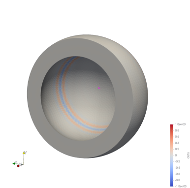
(a) Solution at $t=3$.

(b) Value of $\lambda$ at fixed cell over time.

Figure 6.2: Geometry and solution for the $3d$ example

We solve the sound-soft scattering problem using an indirect ansatz. I.e., we solved the problem of finding $\lambda:[0,T]\to H^{-1/2}(\Gamma)$ such that

$$\partial_{t}V(\partial_{t})\lambda=\dot{g}\qquad\text{in (0,T)},$$

where $\dot{g}$ is a traveling wave, i.e., $\dot{g}(t,x):=\psi(x\cdot d-t)$ with direction $d:=(-1,0.15,0)^{t}$ and profile

$$\psi(\xi):=w_{1}(\xi)\sin(8\pi\xi).$$

We fix the number of timesteps to $15$ and compute up to the end-time $T=8$, giving a timestep size of $0.53$. We then compare the convergence of the method as we increase the polynomial order $p$. Since an exact solution is not available for this problem, we used the finest approximation with $p=36$ as our stand-in. The $H^{-1/2}(\Gamma)$-error was approximated by $\langle V(1)\lambda(t)-\lambda^{k}(t),\lambda(t)-\lambda^{k}(t)\rangle_{\Gamma}$. As $V(1)$ is elliptic this quantity is equivalent to the error. In time, we sampled the solution at a uniform time-grid with $1024$ nodes and took the maximum over all such times. In Figure 6.3, we observe the expected behavior of $\exp(-c\sqrt{p})$ predicted in Corollary 4.8.

Figure 6.3: Convergence for the $3d$ scattering problem

Acknowledgments:

The author gladly acknowledges financial support by the Austrian Science Fund (FWF) through the project P 36150.

References

• [Ban10] L. Banjai. Multistep and multistage convolution quadrature for the wave equation: algorithms and experiments. SIAM J. Sci. Comput., 32(5):2964–2994, 2010.
• [BD86] A. Bamberger and T. H. Duong. Formulation variationnelle pour le calcul de la diffraction d’une onde acoustique par une surface rigide. Math. Methods Appl. Sci., 8(4):598–608, 1986.
• [BHD86] A. Bamberger and T. Ha-Duong. Formulation variationelle espace-temps pour le calcul par potentiel retardé d’une onde acoustique. Math. Meth. Appl. Sci., 8:405–435, 1986.
• [BLS15] L. Banjai, A. R. Laliena, and F.-J. Sayas. Fully discrete Kirchhoff formulas with CQ-BEM. IMA J. Numer. Anal., 35(2):859–884, 2015.
• [BR18] L. Banjai and A. Rieder. Convolution quadrature for the wave equation with a nonlinear impedance boundary condition. Math. Comp., 87(312):1783–1819, 2018.
• [BS09] L. Banjai and S. Sauter. Rapid solution of the wave equation in unbounded domains. SIAM J. Numer. Anal., 47(1):227–249, 2008/09.
• [BS21] T. Betcke and M. W. Scroggs. Bempp-cl: A fast python based just-in-time compiling boundary element library. Journal of Open Source Software, 6(59):2879, 2021.
• [BS22] L. Banjai and F.-J. Sayas. Integral Equation Methods for Evolutionary PDE. Springer International Publishing, 2022. A Convolution Quadrature Approach.
• [GOSS19] H. Gimperlein, C. Özdemir, D. Stark, and E. P. Stephan. $hp$-version time domain boundary elements for the wave equation on quasi-uniform meshes. Comput. Methods Appl. Mech. Engrg., 356:145–174, 2019.
• [GVL13] G. H. Golub and C. F. Van Loan. Matrix computations. Johns Hopkins Studies in the Mathematical Sciences. Johns Hopkins University Press, Baltimore, MD, fourth edition, 2013.
• [HQSVS17] M. E. Hassell, T. Qiu, T. Sánchez-Vizuet, and F.-J. Sayas. A new and improved analysis of the time domain boundary integral operators for the acoustic wave equation. J. Integral Equations Appl., 29(1):107–136, 2017.
• [JR17] P. Joly and J. Rodríguez. Mathematical aspects of variational boundary integral equations for time dependent wave propagation. J. Integral Equations Appl., 29(1):137–187, 2017.
• [LO93] C. Lubich and A. Ostermann. Runge-Kutta methods for parabolic equations and convolution quadrature. Math. Comp., 60(201):105–131, 1993.
• [Lub88a] C. Lubich. Convolution quadrature and discretized operational calculus. I. Numer. Math., 52(2):129–145, 1988.
• [Lub88b] C. Lubich. Convolution quadrature and discretized operational calculus. II. Numer. Math., 52(4):413–425, 1988.
• [McL00] W. McLean. Strongly elliptic systems and boundary integral equations. Cambridge University Press, Cambridge, 2000.
• [MR17] J. M. Melenk and A. Rieder. Runge-Kutta convolution quadrature and FEM-BEM coupling for the time-dependent linear Schrödinger equation. J. Integral Equations Appl., 29(1):189–250, 2017.
• [Mül17] F. Müller. Numerical analysis of finite element methods for second order wave equations in polygons. PhD thesis, ETH Zurich, 2017.
• [Paz83] A. Pazy. Semigroups of linear operators and applications to partial differential equations, volume 44 of Applied Mathematical Sciences. Springer-Verlag, New York, 1983.
• [Rod93] L. Rodino. Linear partial differential operators in Gevrey spaces. World Scientific Publishing Co., Inc., River Edge, NJ, 1993.
• [RSM20] A. Rieder, F.-J. Sayas, and J. M. Melenk. Runge-Kutta approximation for $C_{0}$-semigroups in the graph norm with applications to time domain boundary integral equations. Partial Differ. Equ. Appl., 1(6):Paper No. 49, 47, 2020.
• [RSM22] A. Rieder, F.-J. Sayas, and J. M. Melenk. Time domain boundary integral equations and convolution quadrature for scattering by composite media. Math. Comp., 91(337):2165–2195, 2022.
• [Say16] F.-J. Sayas. Retarded potentials and time domain boundary integral equations, volume 50 of Springer Series in Computational Mathematics. Springer, [Cham], 2016. A road map.
• [Sch98] C. Schwab. $p$- and $hp$-finite element methods. Numerical Mathematics and Scientific Computation. The Clarendon Press, Oxford University Press, New York, 1998. Theory and applications in solid and fluid mechanics.
• [Sch99] D. M. Schotzau. hp-DGFEM for parabolic evolution problems: Applications to diffusion and viscous incompressible fluid flow. ProQuest LLC, Ann Arbor, MI, 1999. Thesis (Dr.Sc.Math)–Eidgenoessische Technische Hochschule Zuerich (Switzerland).
• [SS00a] D. Schötzau and C. Schwab. An $hp$ a priori error analysis of the DG time-stepping method for initial value problems. Calcolo, 37(4):207–232, 2000.
• [SS00b] D. Schötzau and C. Schwab. Time discretization of parabolic problems by the $hp$-version of the discontinuous Galerkin finite element method. SIAM J. Numer. Anal., 38(3):837–875, 2000.
• [SS11] S. A. Sauter and C. Schwab. Boundary element methods, volume 39 of Springer Series in Computational Mathematics. Springer-Verlag, Berlin, 2011. Translated and expanded from the 2004 German original.
• [SV14] S. Sauter and A. Veit. Retarded boundary integral equations on the sphere: exact and numerical solution. IMA J. Numer. Anal., 34(2):675–699, 2014.
• [Tho06] V. Thomée. Galerkin finite element methods for parabolic problems, volume 25 of Springer Series in Computational Mathematics. Springer-Verlag, Berlin, second edition, 2006.
• [Vei11] A. Veit. Numerical methods for time-domain boundary integral equations. PhD thesis, University of Zurich, 2011.
• [Yos80] K. Yosida. Functional analysis, volume 123 of Grundlehren der Mathematischen Wissenschaften. Springer-Verlag, Berlin-New York, sixth edition, 1980.