Learning Topological Representations with Bidirectional Graph Attention Network for Solving Job Shop Scheduling Problem

Abstract

Existing learning-based methods for solving job shop scheduling problem (JSSP) usually use off-the-shelf GNN models tailored to undirected graphs and neglect the rich and meaningful topological structures of disjunctive graphs (DGs). This paper proposes the topology-aware bidirectional graph attention network (TBGAT), a novel GNN architecture based on the attention mechanism, to embed the DG for solving JSSP in a local search framework. Specifically, TBGAT embeds the DG from a forward and a backward view, respectively, where the messages are propagated by following the different topologies of the views and aggregated via graph attention. Then, we propose a novel operator based on the message-passing mechanism to calculate the forward and backward topological sorts of the DG, which are the features for characterizing the topological structures and exploited by our model. In addition, we theoretically and experimentally show that TBGAT has linear computational complexity to the number of jobs and machines, respectively, which strengthens the practical value of our method. Besides, extensive experiments on five synthetic datasets and seven classic benchmarks show that TBGAT achieves new SOTA results by outperforming a wide range of neural methods by a large margin.

1 Introduction

Learning to solve vehicle routing problems (VRP) Golden et al. [2008] has become increasingly popular. In contrast, the job shop scheduling problem (JSSP) Garey et al. [1976], which is more complex, receives relatively less attention.

In most existing research on VRP, fully connected undirected graphs are commonly employed to model the interrelationships between nodes (customers and the depot). This graphical representation enables a range of algorithms to leverage graph neural networks (GNN) for learning problem representations, subsequently facilitating the resolution of VRP Kool et al. [2018], Xin et al. [2021], Joshi et al. [2022]. However, this densely connected topological structure is not applicable to JSSP, as it cannot represent the widespread precedence constraints among operations in a job. As a result, the mainstream research on JSSP utilizes disjunctive graphs (DG) Błażewicz et al. [2000], a sparse and directed graphical model, to depict instances and (partial) solutions. Presently, there are two emerging neural approaches for learning to solve JSSP based on disjunctive graphs. The first neural approach, predominantly featured in existing literature, focuses on learning construction heuristics, which adhere to a dispatching procedure that incrementally develops schedules from partial ones Zhang et al. [2020], Park et al. [2021b, a]. Nonetheless, this method is ill-suited for incorporating diverse work-in-progress (WIP) information (e.g., current machine load and job status) into the disjunctive graph Zhang et al. [2024]. The omission of such crucial information negatively impacts the performance of these construction heuristics. The second neural approach involves learning improvement heuristics for JSSP Zhang et al. [2024], wherein disjunctive graphs represent complete solutions to be refined, effectively transforming the scheduling problem into a graph optimization problem so as to bypass the issues faced by partial schedule representation.

A prevalent approach in the aforementioned research involves utilizing canonical graph neural network (GNN) models, originally designed for undirected graphs, as the foundation for learning disjunctive graph embeddings. We contend that this approach may be inadvisable. Specifically, disjunctive graphs were initially introduced as a class of directed graphs, wherein the arc directions represent the processing order between operations. Notably, when modelling complete solutions, disjunctive graphs transform into directed acyclic graphs (DAGs), with their topological structures (node connectivity) exhibiting a bijective correspondence with the solution (schedule) space Błażewicz et al. [2000]. Learning these structures can substantially assist GNNs in acquiring in-depth knowledge of disjunctive graphs, enabling the differentiation between high-quality and inferior solutions. Nevertheless, conventional GNN models for undirected graphs lack the components necessary to accommodate these topological peculiarities during the learning of representations.

This paper introduces an end-to-end neural local search algorithm for solving JSSP using disjunctive graphs to represent complete solutions. We propose a novel bidirectional graph attention network (TBGAT) tailored for disjunctive graphs, effectively capturing their unique topological features. TBGAT utilizes two independent graph attention modules to learn forward and backward views, incorporating forward and backward topological sorts. The forward view propagates messages from the root to the leaf, considering historical context, while the backward view propagates messages in the opposite direction, incorporating future schedule information. We show that forward topological order in disjunctive graphs corresponds to global processing orderings and present an algorithm for efficient GPU computation. For training, we use the REINFORCE algorithm with entropy regularization. Theoretical analysis and experiments demonstrate TBGAT’s linear computational complexity concerning the number of jobs and machines, a key attribute for practical JSSP solving.

We evaluate our proposed method against a range of neural approaches for JSSP, utilizing five synthetic datasets and seven classic benchmarks. Comprehensive experimental results demonstrate that our TBGAT model attains new state-of-the-art (SOTA) performance across all datasets, significantly surpassing all neural baselines.

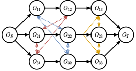
(a) A JSSP instance of size $3\times 3$.

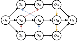
(b) A possible solution.

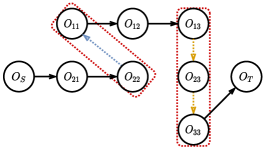
(c) A critical path and the critical blocks on it.

Figure 1: Disjunctive graph representations for JSSP instance and solution.

2 Related Literature

The rapid advancement of artificial intelligence has spurred a growing interest in addressing scheduling-related problems from a machine learning (especially the deep learning) perspective Dogan and Birant [2021]. For JSSP, the neural methods based on deep reinforcement learning (DRL) has emerged as the predominant machine learning paradigm. The majority of existing neural methods for JSSP are construction heuristics that sequentially construct solutions through a decision-making process. L2D Zhang et al. [2020] represents a seminal and exemplary study in this area, wherein a GIN-based Xu et al. [2019] policy learns latent embeddings of partial solutions, represented by disjunctive graphs, and selects operations for dispatch to corresponding machines at each construction step. A similar dispatching procedure is observed in RL-GNN Park et al. [2021b] and ScheduleNet Park et al. [2021a]. To incorporate machine status in decision-making, RL-GNN and ScheduleNet introduce artificial machine nodes with machine-progress information into the disjunctive graph. These augmented disjunctive graphs are treated as undirected, and a type-aware GNN model with two independent modules is proposed for extracting machine and task node embeddings. Despite considerable improvements over L2D, the performance remains suboptimal. DGERD Chen et al. [2022] follows a procedure similar to L2D but with a Transformer-based embedding  networkVaswani et al. [2017]. A recent work, MatNet Kwon et al. [2021], employs an encoding-decoding framework for learning construction heuristics for flexible flow shop problems; however, its assumption of independent machine groups for operations at each stage is overly restrictive for JSSP. JSSenv Tassel et al. [2021] presents a carefully designed and well-optimized simulator for JSSP, extending from the OpenAI gym environment suite Brockman et al. [2016]. Rather than utilizing disjunctive graphs, JSSenv models and represents partial schedule states using Gantt charts Jain and Meeran [1999], and also proposes a DRL agent to solve JSSP instances individually in an online fashion. However, its online nature, requiring training for each instance, results in slower computation than offline-trained methods.

L2S Zhang et al. [2024] significantly narrows the optimality gaps by learning neural improvement heuristics for JSSP, thereby transforming the scheduling problem into a graph structure search problem. Specifically, L2S employs a straightforward local search framework in which a GNN-based agent learns to select pairs of operations for swapping, thus yielding new solutions. The GNN architecture comprises two modules based on GIN Xu et al. [2019] and GAT Veličković et al. [2018], focusing on the disjunctive graph and its subgraphs with different contexts separately. This design introduces two potential issues. Firstly, it is unclear whether GIN can maintain the same discriminative power for directed graphs as for undirected graphs. Secondly, the GAT network cannot allocate distinct attention scores to different neighbours during the representation learning since each node possesses only a single neighbour in either context subgraph, thus rendering the attention mechanism ineffective.

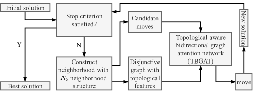
Figure 2: The local search procedure with TBGAT network.

3 Prerequisite

3.1 The job shop scheduling problem.

A JSSP instance of size $|\mathcal{J}|\times|\mathcal{M}|$ comprises a set of jobs $\mathcal{J}$ and a set of machines $\mathcal{M}$. Each job $j\in\mathcal{J}$ must be processed by each machine $m\in\mathcal{M}$ following a predefined order $O_{j1}\rightarrow\cdots\rightarrow O_{ji}\rightarrow\cdots\rightarrow O_{j{|\mathcal{M}|}}$, where $O_{ji}\in\mathcal{O}$ represents the $i$th operation of job $j$. Each operation $O_{ji}$ is allocated to a machine $m_{ji}$ with a processing time $p_{ji}\in\mathbb{N}$. Let $\mathcal{O}_{j}$ and $\mathcal{O}_{m}$ denote the collections of all operations for job $j$ and machine $m$, respectively. The operation $O_{ji}$ can be processed only when all its preceding operations in $\{O_{jk}|k<i\}\subset\mathcal{O}_{j}$ have been completed, which constitutes the precedent constraint. The objective is to identify a schedule $\eta:\mathcal{O}\rightarrow\mathbb{N}$, i.e., the starting time for each operation, that minimizes the makespan $C_{\max}=\max(\eta(O_{ij})+p_{ij})$ without violating the precedent constraints.

3.2 The disjunctive graph representation.

Disjunctive graphs Błażewicz et al. [2000] can comprehensively represent JSSP instances and solutions. As illustrated in Fig. 1(a), a $3\times 3$ JSSP instance is represented by its corresponding disjunctive graph $G=\langle\mathcal{O},\mathcal{C},\mathcal{D}\rangle$. The artificial operations $O_{S}\in\mathcal{O}$ and $O_{T}\in\mathcal{O}$, which possess zero processing time, denote the start and end of the schedule, respectively. The solid arrows represent conjunctions ($\mathcal{C}$), which indicate precedent constraints for each job. The two-headed arrows signify disjunctions ($\mathcal{D}$) that mutually connect all operations belonging to the same machine, forming machine cliques with distinct colors. Discovering a solution is tantamount to assigning directions to disjunctive arcs such that the resulting graph is a directed acyclic graph (DAG) Balas [1969]. For instance, a solution to the JSSP instance in Fig. 1(a) is presented in Fig. 1(b), where the directions of all disjunctive arcs are determined, and the resulting graph is a DAG. Fig. 1(c) emphasizes a critical path of the solution in Fig. 1(b), i.e., the longest path from the source node $O_{S}$ to the sink node $O_{T}$, with critical blocks denoted by red frames. The critical blocks are groups of operations belonging to the same machine on a critical path. The sum of the processing times of operations along the critical path represents the makespan of the solution. Identifying a solution with a smaller makespan is equivalent to finding a disjunctive graph with a shorter critical path.

4 The local search algorithm with proposed TBGAT network

We adopt a neural local search framework akin to L2S Zhang et al. [2024], as depicted in Fig. 2. The process commences with an initial solution produced by a construction heuristic (e.g., the dispatching rule), which is preserved as the current seed and the incumbent (the best-so-far solution). Subsequently, the disjunctive graph representation of the present seed is constructed, and the candidate moves (neighbours) are determined by employing the $N_{5}$ neighbourhood structure Nowicki and Smutnicki [1996]. This structure generates a candidate solution by exchanging the first or last pair of operations in a critical block along a critical path of the disjunctive graph, as demonstrated in Fig. 3. Following Nowicki and Smutnicki [1996], the first pair of operations in the initial critical block and the last pair of operations in the final critical block are excluded. Furthermore, in the presence of multiple critical paths, a random critical path is chosen Zhang et al. [2024], Nowicki and Smutnicki [1996]. The TBGAT network subsequently ingests the disjunctive graph of the current seed as input and produces one of the candidate moves. Ultimately, a new seed solution is acquired by swapping the operations in the disjunctive graph according to the selected operation pair, superseding the incumbent if superior. This search procedure persists until a stopping criterion is met, such as reaching a predetermined horizon, e.g., 5000 steps.

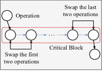
Figure 3: The $N_{5}$ neighborhood structure.

The aforementioned local search procedure can be recast in the framework of the Markov decision process (MDP). Specifically, the state, action, reward, and state transition are delineated as follows.

State. The state $s_{t}$ at time step $t$ represents the disjunctive graph representation of the seed solution at $t$. Action. The action set $A_{t}$ at $t$ comprises the candidate moves of $s_{t}$ calculated by applying the $N_{5}$ neighborhood structure. It is worth noting that $A_{t}$ may be dynamic and contingent on different seed solutions, where $A_{t}=\emptyset$ indicates that the current seed solution is the optimal one Nowicki and Smutnicki [1996]. Reward. The step-wise reward between any two consecutive states $s_{t}$ and $s_{t+1}$ is computed as $r(s_{t},a_{t})=\max\left(C_{\max}(s^{*})-C_{\max}(s_{t+1}),0\right)$, with $s^{*}$ denoting the incumbent. This is well-defined, as maximizing the cumulative reward is tantamount to maximizing the improvement to the initial solution, since $\sum_{t}^{T}r_{t}=C_{\max}(s_{0})-C_{\max}(s_{T})$. State transition. The state $s_{t}$ deterministically transits to the subsequent state $s_{t+1}$ by executing the selected action $a_{t}\in A_{t}$ at $s_{t}$, i.e., exchanging the operation pair in $s_{t}$. The episode terminates if $A_{t}=\emptyset$, beyond which the state transition is ceased.

4.1 The forward and backward views of DGs

Disjunctive graphs (DGs) constitute a specific class of DAGs, exhibiting unique features. Firstly, by adhering to the direction of conjunctive and disjunctive arcs, each node $O_{ji}$ (barring $O_{S}$ and $O_{T}$) has neighbours from two directions. Namely, the predecessors pointing to $O_{ji}$ and successors pointing from $O_{ji}$. Nevertheless, existing GNN-based models either neglect the latter neighbors Zhang et al. [2020, 2024] or fail to differentiate the orientations of neighbors Park et al. [2021b]. In contrast, we recognize that neighbours from both directions are crucial and contain complementary information. Secondly, any $O_{ji}$ in a schedule cannot commence processing earlier than its predecessors, owing to the precedent constraints and the determined machine processing order. The earliest timestamp at which $O_{ji}$ may begin without violating these constraints is defined as the earliest starting time $EST_{ji}$. However, $O_{ji}$ is not mandated to start precisely at $EST_{ji}$ if not delaying the overall makespan. Instead, it has the latest starting time, denoted as $LST_{ji}$. The $EST_{ji}$ and $LST_{ji}$ collectively determine a schedule, which can be calculated recursively from a forward and backward perspective of the disjunctive graph Jungnickel and Jungnickel [2005], respectively, as follows,

$$EST_{ji}=\max_{O_{nl}\in\mathcal{P}_{O_{ji}}}(EST_{nl}+p_{nl}),$$ (1)

$$LST_{ji}=\min_{O_{nl}\in\mathcal{S}_{O_{ji}}}(LST_{nl}-p_{nl}),$$ (2)

where $\mathcal{P}_{O_{ji}}$ and $\mathcal{S}_{O_{ji}}$ represent the sets of predecessors and successors of $O_{ji}$, respectively. In the forward perspective, the computation traverses each $O_{ji}$ by adhering to the directions of conjunctive and disjunctive arcs, which are inverted in the backward perspective. An illustration of the forward and backward perspectives of message flow is demonstrated in Fig. 4.

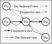
Figure 4: The forward and backward view of the DG.

The processing order of operations intrinsically determines the quality of a schedule, as it defines the message flows of both forward and backward perspectives, represented by the connections of nodes and the orientations of arcs within the graph, i.e., the graph topology. Furthermore, a one-to-one correspondence exists between the space of disjunctive graph topologies and the space of feasible schedules. In other words, each pair of disjunctive graphs possessing distinct topologies corresponds to schedules of differing qualities. Hence, enabling the agent to leverage such topological features to learn discriminative embeddings for various schedules is highly advantageous, as it aids in distinguishing superior schedules from inferior ones. To achieve this, we employ the topological sort Wang et al. [2009], a partial order of nodes in a DAG that depicts their connectivity dependencies, as the topological features. The formal definition of the topological sort of nodes in the disjunctive graph is provided in Definition 1 below.

Definition 1.

(topological sort) Given any disjunctive graph $G=\langle\mathcal{O},\mathcal{C},\mathcal{D}\rangle$, there is a topological sort $\Phi:\mathcal{O}\rightarrow\mathbb{Z}$ such that for any pair of operations $O$ and $O^{\prime}$ if there is an arc (disjunctive or conjunctive) connecting them as $O\rightarrow O^{\prime}$, then $\Phi(O)<\Phi(O^{\prime})$ must hold.

Furthermore, within the context of JSSP, for any two operations $O,O^{\prime}\in\mathcal{O}$, if $O$ is a prerequisite operation of $O^{\prime}$, that is, $O$ must be processed prior to $O^{\prime}$, then $O$ is required to have a higher ranking than $O^{\prime}$ in the topological sort. This demonstrates that the topological sort serves as an alternative representation depicting the processing orders defined by the precedent constraints and the processing sequence of machines. Formally,

Lemma 1.

For any two operations $O_{ji},O_{mk}\in\mathcal{O}$, if $O_{ji}$ is a prerequisite operation of $O_{mk}$, then $\overrightarrow{\Phi}(O_{ji})<\overrightarrow{\Phi}(O_{mk})$ and $EST_{ji}<EST_{mk}$, where $\overrightarrow{\Phi}:\mathcal{O}\rightarrow\mathbb{Z}$ is the topological sort calculated from the forward view of the disjunctive graph.

The proof is in Appendix A. A parallel conclusion can be derived for the backward view of the disjunctive graph, as presented below.

Corollary 1.

For any two operations $O_{ji},O_{mk}\in\mathcal{O}$, if $O_{ji}$ is a prerequisite operation of $O_{mk}$, then $\overleftarrow{\Phi}(O_{ji})>\overleftarrow{\Phi}(O_{mk})$ and $LST_{ji}>LST_{mk}$, where $\overleftarrow{\Phi}:\mathcal{O}\rightarrow\mathbb{Z}$ is the topological sort calculated from the backward view of the disjunctive graph.

The proof is in Appendix B. Our GNN model leverages forward and backward topological sorts to learn latent representations of disjunctive graphs. These sorts capture graph topology and global processing orders (Lemma 1 and Corollary 1). However, traditional algorithms for these sorts pose challenges for DRL agent training due to batch processing complexities, GPU-CPU communication overhead, and DRL data inefficiency. To overcome these issues, we propose MPTS, a novel algorithm based on a message-passing mechanism inspired by GNN computation. MPTS facilitates batch computation of forward and backward topological sorts, ensuring compatibility with GPU processing for more efficient training.

In fact, MPTS is universally applicable to any directed acyclic graph (DAG). Specifically, given a $DAG=\langle\mathcal{O}^{*},\mathcal{E}^{*}\rangle$ with $\mathcal{O}^{*}$ and $\mathcal{E}^{*}$ denoting the sets of nodes and arcs, respectively. Let $\bar{\mathcal{O}}\subset\mathcal{O}^{*}$ be the set of nodes with zero in-degrees, and $\tilde{\mathcal{O}}=\mathcal{O}^{*}\setminus\bar{\mathcal{O}}$ be the set of the remaining nodes, where $\tilde{\mathcal{O}^{\prime}}\subset\tilde{\mathcal{O}}$ is the set of nodes with zero out-degrees. We assign a message $m^{t}_{x}$ to each node $O_{x}\in\mathcal{O}^{*}$, initialized as $m^{0}_{\bar{x}}=0$ for nodes $O_{\bar{x}}\in\bar{\mathcal{O}}$ and $m^{0}_{\tilde{x}}=1$ for nodes $O_{\tilde{x}}\in\tilde{\mathcal{O}}$. Next, we define a message-passing operator $MPO:m^{t}_{x}\rightarrow m^{t+1}_{x}$, which calculates and updates the message for each node $O_{x}$ as $m^{t+1}_{x}=\max_{O_{y}\in\mathcal{N}_{x}}(m^{t}_{y})$, where $\mathcal{N}_{x}$ is a neighborhood of $O_{x}$ containing all nodes $O_{y}$ pointing to $O_{x}$. Finally, let $L$ denote the length of the global longest path in $DAG$, and $L_{x}$ represent the length of any longest path from nodes in the set $O_{\bar{x}}$ to $O_{x}$, we can demonstrate the following.

Theorem 1.

After applying MPO for $L_{x}$ times, $m^{L_{x}}_{x}=1$ for all nodes $O_{x}\in\mathcal{O}$. Moreover, for any pair of nodes $O_{x}$ and $O_{z}$ connected by a path, if $L_{x}<L_{z}\leq L$ then $\Phi(O_{x})<\Phi(O_{z})$.

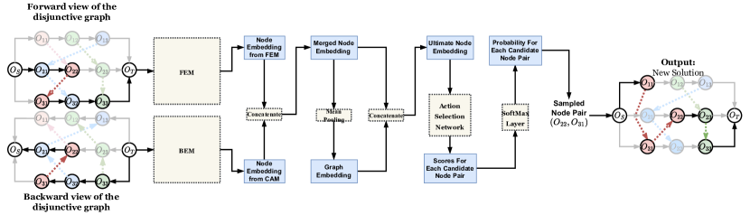
Figure 5: The architecture of the policy network.

The proof is in Appendix C. Theorem 1 suggests an efficient method for computing the topological sort, in which we can iteratively apply the MPO on any $DAG$ and gather the nodes $O_{x}$ with $m^{t}_{x}=1$ at each iteration $0\leq t\leq|\mathcal{O}^{*}|$. Consequently, nodes collected in earlier iterations must hold higher ranks than those in later iterations within the topological sort. Since disjunctive graphs also belong to the class of DAGs, Theorem 1 can be directly applied to compute the forward topological sort $\overrightarrow{\Phi}$, as stated in Lemma 1, and the backward topological sort $\overleftarrow{\Phi}$, as indicated in Corollary 1, respectively. Given that the MPO operator can be readily implemented on a GPU to leverage its powerful parallel computation capabilities, MPO is anticipated to be more efficient than traditional algorithms when handling multiple disjunctive graphs concurrently. To substantiate this assertion, we provide an empirical comparison in the experimental section.

4.2 Graph embedding with TBGAT

In order to effectively learn graph embeddings by leveraging the topological features of disjunctive graphs, we introduce a novel bidirectional graph attention network designed to embed the forward and backward views of the disjunctive graph using two independent modules, respectively. For each view, message propagation adheres to the topology of respective view, and aggregation is accomplished through an attention mechanism, which distinguish our model from previous works. The overarching architecture of the proposed TBGAT is depicted in Fig. 5.

4.2.1 The forward embedding module

In the forward view of the disjunctive graph, each node $O_{x}\in\mathcal{O}$ is associated with a three-dimensional raw feature vector $\overrightarrow{\mathbf{h}}^{0}_{x}=(p_{x},est_{x},\overrightarrow{\Phi}_{x})\in\mathbb{R}^{3}$. Here, $p_{x}$ represents the processing time of node $O_{x}$, $est_{x}$ represents the earliest starting time, and $\overrightarrow{\Phi}_{x}$ represents the forward topological sort of node $O_{x}$. The forward embedding module (FEM) is a graph neural network that consists of $L$ layers. Each layer produces a new message for a node by aggregating the messages of this node and its neighbours from the previous layer. The aggregation operator used for updating the message of node $O_{x}$ is a weighted sum, where the weights are determined by attention scores that indicate the importance of each message. In other words, the aggregation operator for updating the message of node $O_{x}$ is expressed as follows,

$$\overrightarrow{\mathbf{h}}^{l+1}_{x}=\alpha^{l}_{x,x}\mathbf{\theta}^{l}_{ag}\overrightarrow{\mathbf{h}}^{l}_{x}+\sum_{O_{y}\in\mathcal{N}(O_{x})}\alpha^{l}_{x,y}\mathbf{\theta}^{l}_{ag}\overrightarrow{\mathbf{h}}^{l}_{y},0\leq l\leq L-1.$$ (3)

The above attention scores $\alpha^{l}_{x,x}$ and $\alpha^{l}_{x,y}$ are used as weights in the aggregation operator for updating the message of node $O_{x}$ in the forward embedding module (FEM). In specific, $\alpha^{l}_{x,x}$ and $\alpha^{l}_{x,y}$ are the attention scores for the messages of node $O_{x}$ itself and its neighbor $O_{y}$, respectively; $\mathbf{\theta}^{l}_{ag}$ and $\mathcal{N}(x)$ denote the learnable parameters for the aggregation operator and the neighborhood of node $O_{x}$, respectively. Particularly, the two attention scores are computed through a widely-used practice in graph neural networks as follows,

$$\alpha^{l}_{x,*}=\frac{\exp\left(\mathrm{LReLU}\left([\mathbf{a}^{l}]^{\top}[\mathbf{\theta}^{l}_{at}\overrightarrow{\mathbf{h}}^{l}_{x}\,\|\,\mathbf{\theta}^{l}_{at}\overrightarrow{\mathbf{h}}^{l}_{*}]\right)\right)}{\sum_{k\in\mathcal{N}^{\prime}(O_{x})}\exp\left(\mathrm{LReLU}\left([\mathbf{a}^{l}]^{\top}[\mathbf{\theta}^{l}_{at}\overrightarrow{\mathbf{h}}^{l}_{x}\,\|\,\mathbf{\theta}^{l}_{at}\overrightarrow{\mathbf{h}}^{l}_{k}]\right)\right)},$$ (4)

where $||$ denotes the concatenation operator; $*$ refers to $x$ or $y$; $\mathcal{N}^{\prime}(O_{x})=\mathcal{N}(O_{x})\cup\{O_{x}\}$; $\mathrm{LReLU}$ is the LeakyRelU layer Radford et al. [2015]; and $\mathbf{a}^{l}$ and $\mathbf{\theta}^{l}_{at}$ are the learnable parameters.

4.2.2 The backward embedding module

The backward embedding module (BEM) has an architecture that is similar to that of the forward embedding module. However, there is a key difference in the raw feature used for each node. Specifically, the raw feature for each node $O_{x}$ is substituted with the backward hidden state vector $\overleftarrow{\mathbf{h}}^{0}_{x}=(p_{x},lst_{x},\overleftarrow{\Phi}_{x})\in\mathbb{R}^{3}$, where $p_{x}$ represents the processing time of node $O_{x}$, $lst_{x}$ represents the latest starting time of node $O_{x}$, and $\overleftarrow{\Phi}_{x}$ represents the backward topological sort of node $O_{x}$. This allows the backward embedding module to encode the information about the temporal dependencies between nodes in the reverse order of the forward embedding module.

Table 1: Performance on classic benchmarks. “Gap”: the average gap to the best known solutions reported in the previous literature. “Time”: the average time for solving a single instance in seconds (“s”), minutes (“m”), or hours (“h”). For the neural methods, the best results are marked in bold, where the global best results are colored blue.

Method	Taillard																ABZ				FT
	$15\times 15$		$20\times 15$		$20\times 20$		$30\times 15$		$30\times 20$		$50\times 15$		$50\times 20$		$100\times 20$		$10\times 10$		$20\times 15$		$6\times 6$		$10\times 10$		$20\times 5$
	Gap	Time	Gap	Time	Gap	Time	Gap	Time	Gap	Time	Gap	Time	Gap	Time	Gap	Time	Gap	Time	Gap	Time	Gap	Time	Gap	Time	Gap	Time
CP-SAT Perron and Furnon	0.1%	7.7m	0.2%	0.8h	0.7%	1.0h	2.1%	1.0h	2.8%	1.0h	0.0%	0.4h	2.8%	0.9h	3.9%	1.0h	0.0%	0.8s	1.0%	1.0h	0.0%	0.1s	0.0%	4.1s	0.0%	4.8s
L2D Zhang et al. [2020]	24.7%	0.4s	30.0%	0.6s	28.8%	1.1s	30.5%	1.3s	32.9%	1.5s	20.0%	2.2s	23.9%	3.6s	12.9%	28.2s	14.8%	0.1s	24.9%	0.6s	14.5%	0.1s	21.0%	0.2s	36.3%	0.2s
RL-GNN Park et al. [2021b]	20.1%	3.0s	24.9%	7.0s	29.2%	12.0s	24.7%	24.7s	32.0%	38.0s	15.9%	1.9m	21.3%	3.2m	9.2%	28.2m	10.1%	0.5s	29.0%	7.3s	29.1%	0.1s	22.8%	0.5s	14.8%	1.3s
ScheduleNet Park et al. [2021a]	15.3%	3.5s	19.4%	6.6s	17.2%	11.0s	19.1%	17.1s	23.7%	28.3s	13.9%	52.5s	13.5%	1.6m	6.7%	7.4m	6.1%	0.7s	20.5%	6.6s	7.3%	0.2s	19.5%	0.8s	28.6%	1.6s
L2S-500 Zhang et al. [2024]	9.3%	9.3s	11.6%	10.1s	12.4%	10.9s	14.7%	12.7s	17.5%	14.0s	11.0%	16.2s	13.0%	22.8s	7.9%	50.2s	2.8%	7.4s	11.9%	10.2s	0.0%	6.8s	9.9%	7.5s	6.1%	7.4s
TBGAT-500	8.0%	12.6s	9.9%	14.6s	10.0%	17.5s	13.3%	17.2s	16.4%	19.3s	9.6%	23.9s	11.9%	24.4s	6.4%	42.0s	1.1%	9.2s	11.8%	12.8s	0.0%	7.4s	5.2%	10.3s	2.7%	11.7s
Method	LA																SWV						ORB		YN
	$10\times 5$		$15\times 5$		$20\times 5$		$10\times 10$		$15\times 10$		$20\times 10$		$30\times 10$		$15\times 15$		$20\times 10$		$20\times 15$		$50\times 10$		$10\times 10$		$20\times 20$
	Gap	Time	Gap	Time	Gap	Time	Gap	Time	Gap	Time	Gap	Time	Gap	Time	Gap	Time	Gap	Time	Gap	Time	Gap	Time	Gap	Time	Gap	Time
CP-SAT Perron and Furnon	0.0%	0.1s	0.0%	0.2s	0.0%	0.5s	0.0%	0.4s	0.0%	21.0s	0.0%	12.9m	0.0%	13.7s	0.0%	30.1s	0.1%	0.8h	2.5%	1.0h	1.6%	0.5h	0.0%	4.8s	0.5%	1.0h
L2D Zhang et al. [2020]	14.3%	0.1s	5.5%	0.1s	4.2%	0.2s	21.9%	0.1s	24.6%	0.2s	24.7%	0.4s	8.4%	0.7s	27.1%	0.4s	41.4%	0.3s	40.6%	0.6s	30.8%	1.2s	31.8%	0.1s	22.1%	0.9s
RL-GNN Park et al. [2021b]	16.1%	0.2s	1.1%	0.5s	2.1%	1.2s	17.1%	0.5s	22.0%	1.5s	27.3%	3.3s	6.3%	11.3s	21.4%	2.8s	28.4%	3.4s	29.4%	7.2s	16.8%	51.5s	21.8%	0.5s	24.8%	11.0s
ScheduleNet Park et al. [2021a]	12.1%	0.6s	2.7%	1.2s	3.6%	1.9s	11.9%	0.8s	14.6%	2.0s	15.7%	4.1s	3.1%	9.3s	16.1%	3.5s	34.4%	3.9s	30.5%	6.7s	25.3%	25.1s	20.0%	0.8s	18.4%	11.2s
L2S-500 Zhang et al. [2024]	2.1%	6.9s	0.0%	6.8s	0.0%	7.1s	4.4%	7.5s	6.4%	8.0s	7.0%	8.9s	0.2%	10.2s	7.3%	9.0s	29.6%	8.8s	25.5%	9.7s	21.4%	12.5s	8.2%	7.4s	12.4%	11.7s
TBGAT-500	2.1%	2.3s	0.0%	0.9s	0.0%	1.7s	1.8%	9.1s	3.6%	10.8s	5.0%	11.4s	0.0%	4.9s	5.5%	12.1s	23.0%	15.6s	23.7%	17.0s	20.3%	29.8s	7.0%	10.4s	9.6%	14.3s

Table 2: Generalization performance on classic benchmarks. “Gap”: the average gap to the best known solutions reported in the previous literature. “Time”: the average time for solving a single instance in seconds (“s”), minutes (“m”), or hours (“h”). For the neural methods, the best results are marked in bold, where the global best results are colored blue.

Method	Taillard																ABZ				FT
	$15\times 15$		$20\times 15$		$20\times 20$		$30\times 15$		$30\times 20$		$50\times 15$		$50\times 20$		$100\times 20$		$10\times 10$		$20\times 15$		$6\times 6$		$10\times 10$		$20\times 5$
	Gap	Time	Gap	Time	Gap	Time	Gap	Time	Gap	Time	Gap	Time	Gap	Time	Gap	Time	Gap	Time	Gap	Time	Gap	Time	Gap	Time	Gap	Time
CP-SAT Perron and Furnon	0.1%	7.7m	0.2%	0.8h	0.7%	1.0h	2.1%	1.0h	2.8%	1.0h	0.0%	0.4h	2.8%	0.9h	3.9%	1.0h	0.0%	0.8s	1.0%	1.0h	0.0%	0.1s	0.0%	4.1s	0.0%	4.8s
L2S-1000 Zhang et al. [2024]	8.6%	18.7s	10.4%	20.3s	11.4%	22.2s	12.9%	24.7s	15.7%	28.4s	9.0%	32.9s	11.4%	45.4s	6.6%	1.7m	2.8%	15.0s	11.2%	19.9s	0.0%	13.5s	8.0%	15.1s	3.9%	15.0s
L2S-2000 Zhang et al. [2024]	7.1%	37.7s	9.4%	41.5s	10.2%	44.7s	11.0%	49.1s	14.0%	56.8s	6.9%	65.7s	9.3%	90.9s	5.1%	3.4m	2.8%	30.1s	9.5%	39.3s	0.0%	27.2s	5.7%	30.0s	1.5%	29.9s
L2S-5000 Zhang et al. [2024]	6.2%	92.2s	8.3%	1.7m	9.0%	1.9m	9.0%	2.0m	12.6%	2.4m	4.6%	2.8m	6.5%	3.8m	3.0%	8.4m	1.4%	75.2s	8.6%	99.6s	0.0%	67.7s	5.6%	74.8s	1.1%	73.3s
TBGAT-1000	6.1%	24.9s	8.7%	28.7s	9.0%	34.1s	10.9%	33.7s	14.0%	37.3s	7.5%	46.9s	9.4%	47.5s	4.9%	82.3s	1.1%	17.9s	10.1%	25.3s	0.0%	14.2s	4.8%	20.5s	1.1%	23.2s
TBGAT-2000	5.1%	49.7s	7.3%	56.5s	7.9%	67.0s	9.4%	65.9s	12.1%	72.3s	5.6%	92.9s	7.5%	93.7s	3.0%	2.7m	1.1%	35.5s	7.1%	50.0s	0.0%	28.0s	4.7%	41.2s	0.8%	45.8s
TBGAT-5000	4.6%	2.1m	6.3%	2.3m	7.0%	2.7m	6.8%	2.7m	9.7%	2.9m	2.6%	3.9m	5.0%	3.9m	1.2%	6.7m	0.8%	88.2s	6.6%	2.1m	0.0%	69.4s	2.9%	1.7m	0.0%	1.9m
Method	LA																SWV						ORB		YN
	$10\times 5$		$15\times 5$		$20\times 5$		$10\times 10$		$15\times 10$		$20\times 10$		$30\times 10$		$15\times 15$		$20\times 10$		$20\times 15$		$50\times 10$		$10\times 10$		$20\times 20$
	Gap	Time	Gap	Time	Gap	Time	Gap	Time	Gap	Time	Gap	Time	Gap	Time	Gap	Time	Gap	Time	Gap	Time	Gap	Time	Gap	Time	Gap	Time
CP-SAT Perron and Furnon	0.0%	0.1s	0.0%	0.2s	0.0%	0.5s	0.0%	0.4s	0.0%	21.0s	0.0%	12.9m	0.0%	13.7s	0.0%	30.1s	0.1%	0.8h	2.5%	1.0h	1.6%	0.5h	0.0%	4.8s	0.5%	1.0h
L2S-1000 Zhang et al. [2024]	1.8%	14.0s	0.0%	13.9s	0.0%	14.5s	2.3%	15.0s	5.1%	16.0s	5.7%	17.5s	0.0%	20.4s	6.6%	18.2s	24.5%	17.6s	23.5%	19.0s	20.1%	25.4s	6.6%	15.0s	10.5%	23.4s
L2S-2000 Zhang et al. [2024]	1.8%	27.9s	0.0%	28.3s	0.0%	28.7s	1.8%	30.1s	4.0%	32.2s	3.4%	34.2s	0.0%	40.4s	6.3%	35.9s	21.8%	34.7s	21.7%	38.8s	19.0%	49.5s	5.7%	29.9s	9.6%	47.0s
L2S-5000 Zhang et al. [2024]	1.8%	70.0s	0.0%	71.0s	0.0%	73.7s	0.9%	75.1s	3.4%	80.9s	2.6%	85.4s	0.0%	99.3s	5.9%	88.8s	17.8%	86.9s	17.0%	99.8s	17.1%	2.1m	3.8%	75.9s	8.7%	1.9m
TBGAT-1000	1.6%	3.1s	0.0%	1.9s	0.0%	3.3s	1.8%	18.2s	3.5%	21.4s	4.0%	22.8s	0.0%	6.3s	5.3%	24.5s	19.2%	31.2s	20.1%	34.3s	18.5%	59.5s	5.7%	20.8s	8.0%	28.1s
TBGAT-2000	1.5%	4.8s	0.0%	3.7s	0.0%	6.5s	1.6%	36.7s	3.0%	42.4s	2.9%	43.9s	0.0%	8.9s	5.1%	48.9s	14.6%	61.7s	18.1%	67.6s	16.6%	2.0m	5.1%	41.8s	7.0%	55.8s
TBGAT-5000	1.5%	9.8s	0.0%	9.2s	0.0%	16.1s	1.4%	93.1s	2.4%	1.8m	2.1%	52.0s	0.0%	16.9s	4.4%	2.0m	11.1%	2.5m	15.7%	2.7m	14.5%	4.9m	4.5%	1.7m	5.7%	2.3m

4.2.3 Merging the forward and backward embeddings

The merged embedding for a given node $O_{x}$ is derived by concatenating the output vector of the last layer of the forward embedding module (FEM) and the last layer of the backward embedding module (BEM), which results in a single vector that encodes both the forward and backward temporal dependencies of the node as

$$\mathbf{h}^{L}_{x}=\overrightarrow{\mathbf{h}}^{L}_{x}||\overleftarrow{\mathbf{h}}^{L}_{x},\text{for all }O_{x}.$$ (5)

Moreover, we concatenate $\mathbf{h}^{L}_{x}$ with the graph embedding to form the ultimate embedding for each node as

$$\mathbf{h}_{x}=\mathbf{h}^{L}_{x}||\mathbf{h}_{G},\text{for all }O_{x},$$ (6)

where $\mathbf{h}_{G}$ is obtained with the mean pooling of the node embeddings as $\mathbf{h}_{G}=\frac{1}{|\mathcal{O}|}\sum_{O_{x}\in\mathcal{O}}\mathbf{h}_{x}$.

4.3 Action selection

Given the node embeddings $\mathbf{h}_{x}$ and a graph embedding $\mathbf{h}_{G}$, we calculate a “score” for selecting each operation pair in the $N_{5}$ neighborhood structure as follows. For any pair of operations $(O_{x},O_{z})$ obtained from the $N_{5}$ neighborhood structure, we first concatenate the corresponding node embeddings $\mathbf{h}_{x}$ and $\mathbf{h}_{z}$ to obtain the joint representation $\mathbf{h}_{xz}$ for the action $(O_{x},O_{z})$. We then feed $\mathbf{h}_{xz}$ into the action selection network $Net_{A}$, i.e., a multi-layer perceptron (MLP) with $L_{A}$ hidden layers, to obtain a scalar score $sc_{xz}$ for the action $(O_{x},O_{z})$. The score $sc_{xz}$ is then normalized to obtain a probability $p_{xz}$, from which we could sample an action.

4.4 The entropy-regularized REINFORCE algorithm

To train our policy network, we utilize a modified version of the REINFORCE algorithm proposed by Williams Williams [1992]. Our modifications include periodic updates of the policy network parameters, as opposed to updating them only at a fixed step limit $T$. This approach has been shown to improve the generalization of the policy network to larger values of $T$ during testing Zhang et al. [2024]. Additionally, to encourage exploration of the action space, we incorporate a regularization term $\mathcal{H}(\pi_{\theta})=-\mathbb{E}_{a\sim\pi_{\theta}}\log(\pi_{\theta}(a))$ based on the entropy of the policy $\pi_{\theta}$ into the original objective of the REINFORCE algorithm. The complete learning procedure is outlined in Algorithm 1 in Appendix D.

5 Experiment

To comprehensively evaluate the performance of our TBGAT, we conduct a series of experiments on both synthetic and publicly available datasets.

5.1 Experimental setup

The algorithm configurations can be found in Appendix LABEL:algorithm_config.

5.2 Testing datasets and baselines

Datasets. We evaluate the performance of our proposed method on two categories of datasets. The first category comprises synthetic datasets that we generated using the same method as the training dataset. The synthetic dataset includes five different sizes, namely $10\times 10$, $15\times 10$, $15\times 15$, $20\times 10$, and $20\times 15$, each consisting of $100$ instances. The second category includes seven widely used public benchmark datasets, i.e., Taillard Taillard [1993], ABZ Adams et al. [1988], FT Fisher [1963], LA Lawrence [1984], SWV Storer et al. [1992], ORB Applegate and Cook [1991], and YN Yamada and Nakano [1992]. These datasets contain instances with small and large scales, including those not seen during training, such as $100\times 20$, which challenges the generalization ability of our model. It is worth noting that our model is trained with randomly generated synthetic datasets, whereas the seven open benchmark datasets are generated using distributions different from ours. Hence, the results on these classic datasets can be considered the zero-shot generalization performance of our method. We test the model trained on the closest size for each problem size, e.g., the model trained on the size of $10\times 10$ is used for testing on the problem of size $10\times 10$ or others close to it.

Baselines. In order to demonstrate the superior performance of TBGAT, we conduct a comparative analysis against nine different baseline methods of various genres, including eight state-of-the-art neural approaches such as construction heuristics (L2D Zhang et al. [2020], RL-GNN Park et al. [2021b], ScheduleNet Park et al. [2021a], ACL Iklassov et al. [2022], JSSEnv Tassel et al. [2021], and DGERD Chen et al. [2022]), improvement heuristic (L2S Zhang et al. [2024]), and active search (EAS Kwon et al. [2021]). We also include an exact solver, CP-SAT Perron and Furnon , which has been shown to be robust and effective in solving JSSP Da Col and Teppan [2019] when given sufficient computational time ($3600$ seconds). For each problem size, we report the performance of our method in terms of the average relative gap to the best-known solutions, which are available online (for the seven classic benchmark datasets) or computed optimally with CP-SAT (for the synthetic evaluation dataset). For the synthetic datasets, we compare our results against the optimal solution obtained using CP-SAT. The average relative gap is calculated by averaging the gap of each instance, which is defined as follows,

$$\sigma=(C_{max}-C^{*}_{max})/C^{*}_{max}\times 100\%,$$ (7)

where $C^{*}_{max}$ is the best-known solution (for the classic benchmark datasets) or the optimal solution (for the synthetic datasets).

5.3 Performance on public benchmarks

We present the results on public datasets. To present the evaluation results more clearly, we report the results for 500 improvement steps in Table 1 and the generalization results for different numbers of improvement steps in Table 2. In addition to the baselines mentioned earlier, we also include RL-GNN Park et al. [2021b] and ScheduleNet Park et al. [2021a] for comparison. The tables show that TBGAT performs well when generalized to public benchmarks. Specifically, TBGAT achieves the best performance for all problem sizes and datasets, outperforming CP-SAT with a relative gap of 69.2% on Taillard $100\times 20$ instances with a much shorter computational time of 6.7 minutes in Table. 2, compared to 1 hour taken by CP-SAT. Moreover, TBGAT can find optimal solutions for several benchmark datasets with different scales, such as $FT\ 6\times 6$, $LA\ 15\times 5$, $LA\ 20\times 5$, and $LA\ 30\times 10$, while L2S fails to do so. These results confirm that TBGAT achieves state-of-the-art results on the seven classic benchmarks and is relatively robust to different data distributions, as the instances in these datasets are generated using distributions substantially different from our training.

5.4 Comparison with other SOTA baselines

Due to page limit, we leave the comparison against other SOTA baselines in Appendix LABEL:more_results, including ACL Iklassov et al. [2022], JSSEnv Tassel et al. [2021], DGERD Chen et al. [2022]), and active search (EAS Kwon et al. [2021]).

5.5 Ablation study

We conducted an ablation study on the number of attention heads. We also empirically verify the linear computational complexity. Please refer to Appendix LABEL:abstudy for details.

6 Conclusion and future work

We present a novel solution to the job shop scheduling problem (JSSP) using the topological-aware bidirectional graph attention neural network (TBGAT). Our method learns representations of disjunctive graphs by embedding them from both forward and backward views and utilizing topological sorts to enhance topological awareness. We also propose an efficient method to calculate the topological sorts for both views and integrate the TBGAT model into a local search framework for solving JSSP. Our experiments show that TBGAT outperforms a wide range of state-of-the-art neural baselines regarding solution quality and computational overhead. Additionally, we theoretically and empirically show that TBGAT possesses linear time complexity concerning the number of jobs and machines, which is essential for practical solvers.

Learning Topological Representations with Bidirectional Graph Attention Network for Solving Job Shop Scheduling Problem

This Supplementary Material should be submitted together with the main paper.

Appendix A Proof of Lemma 1

$\mathit{Proof.}$ Since $O_{ji}$ is a prerequisite operation of $O_{mk}$, then there exists at least one path from $O_{ji}$ to $O_{mk}$ in the forward view of the disjunctive graph, i.e., $\mathcal{P}_{(O_{ji},O_{mk})}\neq\emptyset$, where $\mathcal{P}_{(O_{ji},O_{mk})}$ denotes the set of all paths from $O_{ji}$ to $O_{mk}$. Then, for any path $P(O_{ji},O_{mk})\in\mathcal{P}_{(O_{ji},O_{mk})}$, by the transitivity of the topological sort, we can get that $\overrightarrow{\Phi}(O_{ji})<\overrightarrow{\Phi}(O_{mk})$. Furthermore, because $\mathcal{P}_{(O_{ji},O_{mk})}\neq\emptyset$, we have $EST_{ji}<EST_{mk}$ due to the precedent constraints and the processing orders given by the disjunctive arcs, i.e., the operations at the head of the arcs always start earlier than that located at the tail of the arcs, which also transits from $O_{ji}$ to $O_{mk}$ by following the path $P(O_{ji},O_{mk})$. $\hfill\square$

Appendix B Proof of Corollary 1

$\mathit{Proof.}$ It is a similar procedure by following the proof of Lemma 1, but with each edge reversed.

Appendix C Proof of Theorem 1

$\mathit{Proof.}$ We show that $m^{L_{x}}_{x}=1$ for all nodes $O_{x}\in\mathcal{O}$. First, it is obvious that $m^{L_{\bar{x}}}_{\bar{x}}=1,\forall O_{\bar{x}}\in\bar{\mathcal{O}}$ since $m^{0}_{\bar{x}}=1$ and $\mathcal{N}_{\bar{x}}=\emptyset$. Second, one can prove that $m^{L_{\tilde{x}}}_{\tilde{x}}=1$ by contradiction. Specifically, if $m^{L_{\tilde{x}}}_{\tilde{x}}\neq 1$, then there must exist a node $O_{\bar{x}^{\prime}}\in\bar{\mathcal{O}}$ connecting to $O_{\tilde{x}}$ via a path, which has message $m_{\bar{x}^{\prime}}\neq 0$, since $L_{x}$ is the maxim length. Hence, it contradicts with $m^{0}_{\bar{x}^{\prime}}=1$. Next, if $L_{x}<L_{z}$ for any pair of nodes $O_{x}$ and $O_{z}$ connected by a path, it is clear that $\Phi(O_{x})<\Phi(O_{z})$ by the definition of the topological sort. $\hfill\square$

Appendix D The Entropy Regularized REINFORCE Algorithm

Algorithm 1 Entropy-regularized REINFORCE

Input: Policy $\pi_{\theta}(a_{t}|s_{t})$, step limit $T$, step size $n$, learning rate $\alpha$, training problem size $|\mathcal{J}|\times|\mathcal{M}|$, batch size $B$, total number of training instances $I$.
Output: Trained policy.

1:  for $i=0$ to $i<I$ do

2:     Randomly generate $B$ instances of size $|\mathcal{J}|\times|\mathcal{M}|$, and compute their initial solutions $\{s_{0}^{1},...,s_{0}^{B}\}$ by using the dispatching rule FDD/MWKR;

3:     for $t=0$ to $T$ do

4:        for $s_{t}^{b}\in\{s_{t}^{1},...,s_{t}^{B}\}$ do

5:           Initialize a training data buffer $D^{b}$ with size 0;

6:           Compute a local move $a^{t}_{b}\sim\pi_{\theta}(a_{t}^{b}|s_{t}^{b})$;

7:           Update $s_{t}^{b}$ w.r.t $a_{t}^{b}$ and receive a reward $r(a_{t}^{b},s_{t}^{b})$;

8:           Store the data $(s_{t}^{b},a_{t}^{b},r(a_{t}^{b},s_{t}^{b}))$ into $D^{b}$;

9:           if $t$ mod $n$ = 0 then

10:              for $j=t,t+1,\cdots,t+n$ do

11:                 $\theta=\theta+lr\nabla_{\theta}\left(\log\pi_{\theta}(a_{j}^{b}|s_{j}^{b})\cdot R_{j}^{b}+{\color[rgb]{0,0,1}\mathcal{H}(\pi_{\theta})}\right)$, where $R_{j}^{b}$ is the return for step $j$, and $\mathcal{H}(\pi_{\theta})$ is the entropy of $\pi_{\theta}$;

12:              end for

13:              Clear buffer $D^{b}$;

14:           end if

15:        end for

16:     end for

17:     $i=i+B$;

18:  end for

19:  return $\theta$;

References

- Adams et al. [1988] Joseph Adams, Egon Balas, and Daniel Zawack. The shifting bottleneck procedure for job shop scheduling. Management Science, 34(3):391–401, 1988.
- Applegate and Cook [1991] David Applegate and William Cook. A computational study of the job-shop scheduling problem. ORSA Journal on Computing, 3(2):149–156, 1991.
- Balas [1969] Egon Balas. Machine sequencing via disjunctive graphs: an implicit enumeration algorithm. Operations research, 17(6):941–957, 1969.
- Błażewicz et al. [2000] Jacek Błażewicz, Erwin Pesch, and Małgorzata Sterna. The disjunctive graph machine representation of the job shop scheduling problem. European Journal of Operational Research, 127(2):317–331, 2000.
- Brockman et al. [2016] Greg Brockman, Vicki Cheung, Ludwig Pettersson, Jonas Schneider, John Schulman, Jie Tang, and Wojciech Zaremba. Openai gym. arXiv preprint arXiv:1606.01540, 2016.
- Chen et al. [2022] Ruiqi Chen, Wenxin Li, and Hongbing Yang. A deep reinforcement learning framework based on an attention mechanism and disjunctive graph embedding for the job shop scheduling problem. IEEE Transactions on Industrial Informatics, 2022.
- Da Col and Teppan [2019] Giacomo Da Col and Erich C Teppan. Industrial size job shop scheduling tackled by present day cp solvers. In International Conference on Principles and Practice of Constraint Programming, pages 144–160. Springer, 2019.
- Dogan and Birant [2021] Alican Dogan and Derya Birant. Machine learning and data mining in manufacturing. Expert Systems with Applications, 166:114060, 2021.
- Fey and Lenssen [2019] Matthias Fey and Jan Eric Lenssen. Fast graph representation learning with pytorch geometric. arXiv preprint arXiv:1903.02428, 2019.
- Fisher [1963] Henry Fisher. Probabilistic learning combinations of local job-shop scheduling rules. Industrial Scheduling, pages 225–251, 1963.
- Garey et al. [1976] Michael R Garey, David S Johnson, and Ravi Sethi. The complexity of flowshop and jobshop scheduling. Mathematics of operations research, 1(2):117–129, 1976.
- Golden et al. [2008] Bruce L Golden, Subramanian Raghavan, Edward A Wasil, et al. The vehicle routing problem: latest advances and new challenges, volume 43. Springer, 2008.
- Hottung et al. [2021] André Hottung, Yeong-Dae Kwon, and Kevin Tierney. Efficient active search for combinatorial optimization problems. In International Conference on Learning Representations, 2021.
- Iklassov et al. [2022] Zangir Iklassov, Dmitrii Medvedev, Ruben Solozabal, and Martin Takac. Learning to generalize dispatching rules on the job shop scheduling. arXiv preprint arXiv:2206.04423, 2022.
- Jain and Meeran [1999] Anant Singh Jain and Sheik Meeran. Deterministic job-shop scheduling: Past, present and future. European journal of operational research, 113(2):390–434, 1999.
- Joshi et al. [2022] Chaitanya K Joshi, Quentin Cappart, Louis-Martin Rousseau, and Thomas Laurent. Learning the travelling salesperson problem requires rethinking generalization. Constraints, pages 1–29, 2022.
- Jungnickel and Jungnickel [2005] Dieter Jungnickel and D Jungnickel. Graphs, networks and algorithms, volume 3. Springer, 2005.
- Kool et al. [2018] Wouter Kool, Herke van Hoof, and Max Welling. Attention, learn to solve routing problems! In International Conference on Learning Representations, 2018.
- Kwon et al. [2021] Yeong-Dae Kwon, Jinho Choo, Iljoo Yoon, Minah Park, Duwon Park, and Youngjune Gwon. Matrix encoding networks for neural combinatorial optimization. In M. Ranzato, A. Beygelzimer, Y. Dauphin, P.S. Liang, and J. Wortman Vaughan, editors, Advances in Neural Information Processing Systems, volume 34, pages 5138–5149. Curran Associates, Inc., 2021. URL https://proceedings.neurips.cc/paper/2021/file/29539ed932d32f1c56324cded92c07c2-Paper.pdf.
- Lawrence [1984] Stephen Lawrence. Resouce constrained project scheduling: An experimental investigation of heuristic scheduling techniques (supplement). Graduate School of Industrial Administration, Carnegie-Mellon University, 1984.
- Nowicki and Smutnicki [1996] Eugeniusz Nowicki and Czeslaw Smutnicki. A fast taboo search algorithm for the job shop problem. Management science, 42(6):797–813, 1996.
- Park et al. [2021a] Junyoung Park, Sanjar Bakhtiyar, and Jinkyoo Park. Schedulenet: Learn to solve multi-agent scheduling problems with reinforcement learning. arXiv preprint arXiv:2106.03051, 2021a.
- Park et al. [2021b] Junyoung Park, Jaehyeong Chun, Sang Hun Kim, Youngkook Kim, Jinkyoo Park, et al. Learning to schedule job-shop problems: representation and policy learning using graph neural network and reinforcement learning. International Journal of Production Research, 59(11):3360–3377, 2021b.
- Paszke et al. [2019] Adam Paszke, Sam Gross, Francisco Massa, Adam Lerer, James Bradbury, Gregory Chanan, Trevor Killeen, Zeming Lin, Natalia Gimelshein, Luca Antiga, et al. Pytorch: An imperative style, high-performance deep learning library. Advances in neural information processing systems, 32, 2019.
- [25] Laurent Perron and Vincent Furnon. Or-tools. URL https://developers.google.com/optimization/.
- Radford et al. [2015] Alec Radford, Luke Metz, and Soumith Chintala. Unsupervised representation learning with deep convolutional generative adversarial networks. arXiv preprint arXiv:1511.06434, 2015.
- Storer et al. [1992] Robert H Storer, S David Wu, and Renzo Vaccari. New search spaces for sequencing problems with application to job shop scheduling. Management Science, 38(10):1495–1509, 1992.
- Taillard [1993] Eric Taillard. Benchmarks for basic scheduling problems. European Journal of Operational Research, 64(2):278–285, 1993.
- Tassel et al. [2021] Pierre Tassel, Martin Gebser, and Konstantin Schekotihin. A reinforcement learning environment for job-shop scheduling. arXiv preprint arXiv:2104.03760, 2021.
- Vaswani et al. [2017] Ashish Vaswani, Noam Shazeer, Niki Parmar, Jakob Uszkoreit, Llion Jones, Aidan N Gomez, Łukasz Kaiser, and Illia Polosukhin. Attention is all you need. Advances in neural information processing systems, 30, 2017.
- Veličković et al. [2018] Petar Veličković, Guillem Cucurull, Arantxa Casanova, Adriana Romero, Pietro Liò, and Yoshua Bengio. Graph attention networks. In International Conference on Learning Representations, 2018.
- Wang et al. [2009] Laung-Terng Wang, Yao-Wen Chang, and Kwang-Ting Tim Cheng. Electronic design automation: synthesis, verification, and test. Morgan Kaufmann, 2009.
- Williams [1992] Ronald J Williams. Simple statistical gradient-following algorithms for connectionist reinforcement learning. Machine learning, 8(3):229–256, 1992.
- Xin et al. [2021] Liang Xin, Wen Song, Zhiguang Cao, and Jie Zhang. Multi-decoder attention model with embedding glimpse for solving vehicle routing problems. In Proceedings of 35th AAAI Conference on Artificial Intelligence, pages 12042–12049, 2021.
- Xu et al. [2019] Keyulu Xu, Weihua Hu, Jure Leskovec, and Stefanie Jegelka. How powerful are graph neural networks? In International Conference on Learning Representations, 2019. URL https://openreview.net/forum?id=ryGs6iA5Km.
- Yamada and Nakano [1992] Takeshi Yamada and Ryohei Nakano. A genetic algorithm applicable to large-scale job-shop problems. In PPSN, volume 2, pages 281–290, 1992.
- Zhang et al. [2020] Cong Zhang, Wen Song, Zhiguang Cao, Jie Zhang, Puay Siew Tan, and Xu Chi. Learning to dispatch for job shop scheduling via deep reinforcement learning. In H. Larochelle, M. Ranzato, R. Hadsell, M. F. Balcan, and H. Lin, editors, Advances in Neural Information Processing Systems, volume 33, pages 1621–1632. Curran Associates, Inc., 2020. URL https://proceedings.neurips.cc/paper/2020/file/11958dfee29b6709f48a9ba0387a2431-Paper.pdf.
- Zhang et al. [2024] Cong Zhang, Zhiguang Cao, Wen Song, Yaoxin Wu, and Jie Zhang. Deep reinforcement learning guided improvement heuristic for job shop scheduling. In The Twelfth International Conference on Learning Representations, 2024. URL https://openreview.net/forum?id=jsWCmrsHHs.