One-loop corrections in Maxwell-metric-affine bumblebee gravity

Abstract

In this paper, we consider the coupling of the metric-affine bumblebee gravity to the Abelian gauge field and obtain the effective model corresponding to the weak gravity limit of this theory. The effective bumblebee theory displays new unconventional couplings between the bumblebee field and its field strength, and the $U(1)$ gauge field along with its respective field strength, as a result of the non-metricity effects. Thus, being a new gauge-bumblebee theory, it represents an example of vector-vector couplings which are very rarely considered, if not entirely overlooked, in the Abelian case. For this theory we calculate the lower perturbative corrections. We close the paper with discussions of other possible vector-vector couplings.

I Introduction

As it is well known, spontaneous symmetry breaking mechanism is one of the most powerful ways to violate Lorentz symmetry within various field theories, especially in gravity (for discussions, see f.e. KosLiGrav and references therein). Indeed, within this approach one does not need to introduce an a priori constant vector (it must be noted that, in general, constant vectors cannot be consistently defined in a curved spacetime KosLiGrav ), but, instead of this, the Lorentz symmetry is broken through arising of some non-trivial vacuum of a bumblebee potential KosGra . We note that namely this mechanism was assumed originally in KosSam to introduce a possibility for the Lorentz symmetry breaking (LSB) itself. It is interesting not only in a curved spacetime but also in a flat one as well. Therefore, the natural task is to consider more generic field theory models involving different fields coupled to a bumblebee field, both at classical and quantum levels.

Earlier, one of the main interests within the LSB context was called by the bumblebee-spinor models in flat spacetime allowing for dynamical LSB, so that the one-loop effective potential arises as a fermionic determinant dyn1 , dyn2 , dyn3 . Another pivotal topic we need to bring to bear is the incorporation of (local) LSB in the context of gravitational theories. Fortunately, a consistent way to implement LSB in curved space-times has already been developed in KosGra . In this work, the authors propose a general framework laying out all possible Lorentz-violating operators in the pure-gravity sector of the Standard Model Extension (SME) which is defined in a Riemann-Cartan manifold. Furthermore, they present the bumblebee gravity model as an example of a modified theory of gravity with spontaneous LSB. Although such a model was originally scrutinized in the Riemann-Cartan background, a flurry of works has addressed it in the standard pseudo-Riemannian background C , D , E , F , G , H , L , M . However, as it is well known, taking a more generic geometrical approach than the usual metric one, we mean considering non-Riemannian geometries, might be a promising way to explore further theoretical and phenomenological consequences of the LSB within modified theories of gravity. To go forward in this subject, the authors of ourbumb2019 proposed a metric-affine extension of the bumblebee gravity model called metric-affine bumblebee gravity. From the theoretical perspective, they have obtained new unusual vector-spinor and vector-scalar couplings to arise within this model ourbumb2019 . These theories, afterwards, have been treated perturbatively ourbumb2 , ourbumb3 , and some studies of perturbative aspects of the bumblebee field coupled to other fields are presented also in Maluf1 , Maluf2 . From the phenomenological perspective, exact solutions describing rotating and non-rotating black holes with LSB have been obtained within this model Filho:2022yrk , Filho:2024hri , and the upper bound limits of the Lorentz-violating (LV) parameter have been estimated by confronting the theoretical results with the astrophysics experimental data at disposal Filho:2022yrk , Filho:2024hri .

Therefore, due to the richness of the metric-affine bumblebee gravity model, the natural continuation of the aforementioned studies consists in coupling the bumblebee field to a gauge field. In this paper, we pursue this aim. Explicitly, we formulate a theory where the metric-affine bumblebee gravity is coupled to a gauge field, consider the weak gravity limit of this theory, obtaining, as a result, the effective bumblebee-gauge theory, and calculate lower quantum corrections in it.

The structure of this paper looks like as follows. In section II, we briefly review the main aspects of the metric-affine bumblebee gravity and formulate our model. In section III, we proceed with the quantum corrections of the effective metric-affine bumblebee model coupled with a gauge field in the weak field approximation and expanded up to the second order in the non-minimal coupling. In section IV, we summarize our results.

II Bumblebee model in Palatini approach

We start our study by writing the bumblebee action in a curved space-time (cf. f.e. Seifert ):

$$S_{B} = \int d^{4}x\,\sqrt{-g}\Big{[}\frac{1}{2\kappa^{2}}\Big{(}R(\Gamma)+\xi B^{\alpha}B^{\beta}R_{\alpha\beta}(\Gamma)\Big{)}-\frac{1}{4}B^{\mu\nu}B_{\mu\nu}-V(B^{\mu}B_{\mu}\pm b^{2})\Big{]}+$$ (1)

$$+ \int d^{4}x\,\sqrt{-g}\mathcal{L}_{M}(g_{\mu\nu},A_{\nu}),$$

where $\sqrt{-g}$ is the determinant of the metric $g_{\mu\nu}$, $\mathcal{L}_{M}(g_{\mu\nu},A_{\nu})$ is the Lagrangian involving all non-gravitational fields, in our case, the electromagnetic field, and $\xi$ is the constant characterizing the non-minimal coupling between the bumblebee field and geometry of space-time. Here we assume that the gravitational sector of (1) is defined in the metric-affine approach in which the connection $\Gamma^{\mu}_{\nu\lambda}$ and metric $g_{\mu\nu}$ are independent dynamical fields a priori.

Another ingredient is the bumblebee field $B_{\mu}$ introduced in order to break the Lorentz symmetry spontaneously KosGra . We remark the presence of the non-minimal coupling between the bumblebee and the Ricci tensor (the second term in the r.h.s. of (1)) which will play an important role in the following. The potential $V(B^{\mu}B_{\mu}\mp b^{2})$ is chosen in such a way that the bumblebee field $B_{\mu}$ acquires the non-zero expectation value (VEV) given by some vector whose presence introduces the privileged direction in the space-time, hence resulting in a spontaneous Lorentz symmetry breaking. Explicitly, we use the most natural form for this potential, that is, $V=\frac{\lambda}{4}(B^{\mu}B_{\mu}\mp b^{2})^{2}$, here and further, the $\mp$ sign reflects the fact that the $B_{\mu}$ can be both space-like and time-like, while $b^{2}>0$. Further, we shall denote the bumblebee field strength associated to $B_{\mu}$ by $B_{\mu\nu}$, and its explicit form is defined below

$$B_{\mu\nu} \equiv \ (dB)_{\mu\nu}=\partial_{\mu}B_{\nu}-\partial_{\nu}B_{\mu}.$$ (2)

Here, for the sake of the simplicity, we assumed the zero torsion case similarly to the previous papers ourbumb2019 , ourbumb2 , hence, the affine connection is symmetric. The electromagnetic field Lagrangian is assumed to be the usual one

$${\cal L}_{A}=-\frac{1}{4}\sqrt{-g}F_{\mu\nu}F^{\mu\nu}.$$ (3)

The equations of motion in our theory, for a generic external fields (their role in our case is played by the electromagnetic field) look like ourbumb2 :

$$0 = R_{(\mu\nu)}(\Gamma)-\frac{1}{2}g_{\mu\nu}\bigg{(}R(\Gamma)+\xi B^{\alpha}B^{\beta}R_{\alpha\beta}(\Gamma)\bigg{)}++2\xi\bigg{(}B_{(\mu}R_{\nu)\beta}(\Gamma)\bigg{)}B^{\beta}=\kappa^{2}T_{\mu\nu},$$

$$0 = \nabla_{\lambda}^{(\Gamma)}\bigg{[}\sqrt{-g}g^{\mu\alpha}\bigg{(}\delta^{\nu}_{\alpha}+\xi B^{\nu}B_{\alpha}\bigg{)}\bigg{]},$$

$$\nabla_{\mu}^{(g)}B^{\mu\nu} = -\frac{\xi}{\kappa^{2}}g^{\nu\alpha}B^{\beta}R_{\alpha\beta}(\Gamma)+2V^{\prime}B^{\nu},$$ (4)

where $T_{\mu\nu}=T_{\mu\nu}^{M}+T_{\mu\nu}^{B}$ described the contributions of the matter sources $T_{\mu\nu}^{M}$ (in our case this is just the energy-momentum tensor of the electromagnetic field) and of the bumblebee field, namely

$$T_{\mu\nu}^{M} = -\frac{2}{\sqrt{-g}}\frac{\delta(\sqrt{-g}\mathcal{L}_{M})}{\delta g^{\mu\nu}},$$ (5)

$$T_{\mu\nu}^{B} = B_{\mu\sigma}B_{\nu}^{\ \sigma}-\frac{1}{4}g_{\mu\nu}B^{\alpha}_{\ \sigma}B^{\sigma}_{\ \alpha}-Vg_{\mu\nu}+2V^{\prime}B_{\mu}B_{\nu}.$$ (6)

The equation of motion for the connection (the second one in (4)) in our case is the purely algebraic one, its solution is given by the Levi-Civita connection of the auxiliary metric $h_{\mu\nu}$ defined by

$$h_{\mu\nu}=\sqrt{1+\xi X}\left(g_{\mu\nu}-\frac{\xi}{1+\xi X}B_{\mu}B_{\nu}\right),$$ (7)

and, its inverse,

$$h^{\mu\nu}=\frac{1}{\sqrt{1+\xi X}}\left(g^{\mu\nu}+\xi B^{\mu}B^{\nu}\right),$$ (8)

where $X\equiv g^{\mu\nu}B_{\mu}B_{\nu}$. Now, in order to proceed with a perturbative description of our theory, we assume particle physics scenarios that correspond to the weak gravitational field regime. In this context, the auxiliary metric $h_{\mu\nu}=\eta_{\mu\nu}$. On the other hand, the physical (spacetime) metric $g_{\mu\nu}$ gets local contributions of the energy density stemming from the bumblebee field whose explicit form in the weak-field limit, up to second-order in $\xi$, is

$$g_{\mu\nu}=\eta_{\mu\nu}+\xi(B_{\mu}B_{\nu}-\frac{1}{2}B^{2}\eta_{\mu\nu})+\xi^{2}B^{2}\left(\frac{5}{8}\eta_{\mu\nu}B^{2}-B_{\mu}B_{\nu}\right),$$ (9)

and its inverse

$$g^{\mu\nu}=\eta^{\mu\nu}+\xi(\frac{1}{2}B^{2}\eta^{\mu\nu}-B^{\mu}B^{\nu})+\xi^{2}B^{2}\left(B^{\mu}B^{\nu}-\frac{3}{8}\eta^{\mu\nu}B^{2}\right),$$ (10)

where $B^{2}\equiv\eta^{\mu\nu}B_{\mu}B_{\nu}$. Substituting this solution in the electromagnetic Lagrangian (3), we find

$${\cal L}_{A} = -\frac{1}{4}F_{\mu\nu}F^{\mu\nu}-\frac{1}{8}\xi B^{2}F_{\mu\nu}F^{\mu\nu}+\frac{\xi}{2}B^{\mu}F_{\mu\nu}B_{\lambda}F^{\lambda\nu}+\frac{3}{32}\xi^{2}B^{4}F^{\mu\nu}F_{\mu\nu}-$$ (11)

$$- \frac{\xi^{2}}{2}B^{2}F^{\mu\beta}F_{\mu\nu}B^{\nu}B_{\beta}+O(\xi^{3}).$$

We note that the third term in this expression is nothing more than the aether term CarTam , ouraether . This action should be summed with the bumblebee action in the weak gravity limit ourbumb2 and expanded up to second order in $\xi$ by using Eqs. (9,10), thus

$${\cal L}_{BEF} = -\frac{1}{4}B_{\mu\nu}B^{\mu\nu}+\frac{M^{2}}{2}B^{2}-\frac{\Lambda}{4}(B^{2})^{2}$$ (12)

$$+ \frac{\xi}{4}\left[\lambda B^{6}-2\lambda(\pm B^{2}-b^{2})(B^{\mu}b_{\mu})^{2}-\frac{1}{2}B^{2}B_{\mu\nu}B^{\mu\nu}+2B^{\mu}_{\phantom{a}\beta}B_{\mu\nu}B^{\nu}B^{\beta}\right]$$

$$+ \frac{\xi^{2}}{8}\bigg{[}\lambda(-B^{8}\pm 4B^{4}(B^{\mu}b_{\mu})^{2}-2(B^{\mu}b_{\mu})^{4}\mp\frac{9}{2}B^{6}b^{2})+\frac{3}{4}B^{4}B_{\mu\nu}B^{\mu\nu}-$$

$$- 4B^{2}B^{\mu\beta}B_{\mu\nu}B^{\nu}B_{\beta}\bigg{]}+\mathcal{O}(\xi^{3}),$$

where we have defined the quantities $M^{2}=\lambda b^{2}(\pm 1-\frac{1}{2}\xi b^{2})$ and $\Lambda=\lambda(1-\frac{7}{4}b^{4}\xi^{2})$. It should be realized that the above Lagrangian is more generic than the one considered in ourbumb2 , where terms proportional to $\xi^{2}$ and $\xi\lambda$ were disregarded. So, we can study various aspects of the theory formed by the sum ${\cal L}_{A}+{\cal L}_{BEF}$, for example exact solutions and quantum corrections.

We consider the simple propagator

$$<B_{\mu}B_{\nu}>=-\frac{i\eta_{\mu\nu}}{k^{2}-M^{2}},$$ (13)

while the LV background will be treated as a perturbation. This scheme is different from the one used in the previous paper ourbumb2 .

III Radiative corrections

We can calculate various perturbative contributions in the effective theory. Initially, we focus on deriving the contribution involving external gauge legs, with the bumblebee field is integrated out, and further, we obtain the bumblebee-dependent corrections. To study the lower quantum contributions in our theory, we restrict our calculation to the order of $\xi^{2}$.

III.1 The photon self-energy

Let us begin the computation of the radiative corrections to the photon self-energy. The diagrams contributing to this process are illustrated in Figure 1. The expression for the diagram 1.1 is given by

$$\Pi^{\mu\nu}_{A1.1}(p) = \int{\frac{d^{D}k}{(2\pi)^{D}}}\frac{\xi g_{\alpha\gamma}}{2\left(k^{2}-M^{2}\right)}\Big{[}p^{\mu}p^{\nu}g^{\alpha\gamma}-p^{2}g^{\alpha\gamma}g^{\mu\nu}-p^{\alpha}p^{\mu}g^{\nu\gamma}-p^{\alpha}p^{\nu}g^{\mu\gamma}$$ (14)

$$-p^{\gamma}p^{\mu}g^{\nu\alpha}-p^{\gamma}p^{\nu}g^{\mu\alpha}+2p^{\alpha}p^{\gamma}g^{\mu\nu}+p^{2}g^{\nu\alpha}g^{\mu\gamma}+p^{2}g^{\mu\alpha}g^{\nu\gamma}\Big{]}$$

$$= \frac{iM^{2}\xi\left(p^{2}g^{\mu\nu}-p^{\mu}p^{\nu}\right)}{16\pi^{2}}.$$

Notice that this contribution is UV finite.

This contribution merely generates a finite correction to the Maxwell effective action, as

$$S_{M}=-\frac{1}{4}\int{d^{4}x}\leavevmode\nobreak\ \left(1-\frac{\xi M^{2}}{16\pi^{2}}\right)F^{\mu\nu}F_{\mu\nu}.$$ (15)

Now, let us proceed to calculate the impacts of the insertion of the LV vertices. The corresponding diagrams are depicted in Figure 1.2-4. The expression for the polarization tensor can be written as

$$\Pi^{\mu\nu}_{A}(p) = \frac{i\xi(2\Lambda-\xi M^{2})}{8\pi^{2}\epsilon}\left[-g^{\mu\nu}(b\cdot p)^{2}-p^{2}b^{\mu}b^{\nu}+b^{\nu}p^{\mu}(b\cdot p)+b^{\mu}p^{\nu}(b\cdot p)\right]$$ (16)

$$+\frac{i\xi b^{2}(\Lambda+\xi M^{2})}{8\pi^{2}\epsilon}\left(p^{2}g^{\mu\nu}-p^{\mu}p^{\nu}\right)+\mathrm{finite},$$

where $\epsilon=(4-D)/2$ with $D$ being the dimension of the spacetime.

The corresponding UV divergent component of the expression to the quadratic part of the effective action can be cast as

$$S_{eff} = \int{d^{4}x}\Big{\{}\frac{\xi b^{2}(\Lambda+\xi M^{2})}{32\pi^{2}\epsilon}F^{\mu\nu}F_{\mu\nu}-\frac{\xi(2\Lambda-\xi M^{2})}{32\pi^{2}\epsilon}b^{\mu}F_{\mu\nu}b_{\rho}F^{\rho\nu}\Big{\}}.$$ (17)

Therefore we have corrections to the Maxwell term and to the aether term.

III.2 The Euler-Heisenberg effective action

Our next objective is to calculate the photon 4-point amplitude, which is associated with the Euler-Heisenberg (EH) effective action. In the symmetric phase, the diagrams contributing to this amplitude are depicted in the Fig. 2. The corresponding one-loop EH effective action in the case of small external momenta is given by

$$S_{EH} = \int{d^{4}x}\frac{\xi^{2}}{16(2\pi)^{2}}\mathrm{\bf B}_{0}(0,M^{2},M^{2})\left[-\frac{1}{4}(F^{\mu\nu}F_{\mu\nu})^{2}+F^{\mu\nu}F_{\nu\rho}F^{\rho\sigma}F_{\sigma\mu}\right]$$ (18)

$$= \int{d^{4}x}\left(\frac{\xi^{2}}{64\pi^{2}\epsilon}+\mathrm{finite}\right)\left[-\frac{1}{4}(F^{\mu\nu}F_{\mu\nu})^{2}+F^{\mu\nu}F_{\nu\rho}F^{\rho\sigma}F_{\sigma\mu}\right],$$

where

$$\mathrm{\bf B}_{0}(0,M^{2},M^{2})=\frac{1}{\pi^{2}}\int\frac{d^{D}k}{(k^{2}-M^{2})^{2}}=\frac{1}{\varepsilon}+\ln\left(\frac{\mu^{2}\mathrm{e}^{-\gamma_{E}}}{\pi M^{2}}\right)$$ (19)

with $\gamma_{E}$ being the Euler-Mascheroni constant.

The UV divergence presented in Eq. (18) highlights the need for incorporating an EH counterterm, as anticipated. This is in line with expectations, given that our model is nonrenormalizable and should be treated as an effective field theory.

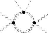
Figure 3: Topology of one-loop corrections to the Lorentz-violating four-photon amplitude up to order $\xi^{2}$.

In the LV broken phase, the corresponding LV EH effective action is derived from the diagrams depicted in the Fig. 3. The expression for small external momenta corresponding to this action can be written as:

$$S_{LVEH} = \int{d^{4}x}\frac{\Lambda\xi^{2}}{32\pi^{2}M^{2}}\Big{\{}b_{\mu}b^{\tau}\left[-\frac{1}{2}F^{\mu\nu}F_{\tau\nu}F^{\rho\sigma}F_{\rho\sigma}+F^{\mu\nu}F_{\nu\rho}F^{\rho\sigma}F_{\sigma\tau}\right]$$ (20)

$$+b^{2}\left[-\frac{1}{4}(F^{\mu\nu}F_{\mu\nu})^{2}+F^{\mu\nu}F_{\nu\rho}F^{\rho\sigma}F_{\sigma\mu}\right]\Big{\}}.$$

It is worth noting that the LV EH effective action is UV finite. The first two terms correspond to an aether-like contribution to the EH action, while the term proportional to $b^{2}$ represents a UV finite Lorentz-invariant correction to the standard EH effective action.

III.3 The bumblebee field self-energy

Now we shall compute the self-energy of the bumblebee field corresponding to the Feynman diagram depicted in Fig. 4. To start, we shall obtain the expressions associated with 4.1 and 4.2. The Lorentz invariant part of the UV divergent contribution is given by

$$\Pi^{\mu\nu}_{B}(p)=-\frac{3i\Lambda M^{2}g^{\mu\nu}}{8\pi^{2}\epsilon}.$$ (21)

Next, we calculate the LV corrections to the self-energy of the bumblebee field, depicted in Fig. 4. These diagrams exhibit the following UV divergent part

$$\Pi^{\mu\nu}_{B}(p) = -\frac{7\Lambda\xi g^{\mu\nu}(b\cdot p)^{2}}{12\pi^{2}\epsilon}+\frac{9\Lambda\xi b^{\nu}p^{\mu}(b\cdot p)}{8\pi^{2}\epsilon}+\frac{9\Lambda\xi b^{\mu}p^{\nu}(b\cdot p)}{8\pi^{2}\epsilon}+\frac{3b^{2}\Lambda^{2}g^{\mu\nu}}{2\pi^{2}\epsilon}$$ (22)

$$+\frac{23b^{2}\lambda M^{2}\xi g^{\mu\nu}}{8\pi^{2}\epsilon}-\frac{3b^{2}\Lambda M^{2}\xi g^{\mu\nu}}{8\pi^{2}\epsilon}+\frac{7b^{2}\Lambda\xi p^{2}g^{\mu\nu}}{24\pi^{2}\epsilon}-\frac{5b^{2}\Lambda\xi p^{\mu}p^{\nu}}{24\pi^{2}\epsilon}$$

$$+\frac{3\Lambda^{2}b^{\mu}b^{\nu}}{\pi^{2}\epsilon}+\frac{5\lambda M^{2}\xi b^{\mu}b^{\nu}}{\pi^{2}\epsilon}-\frac{3\Lambda M^{2}\xi b^{\mu}b^{\nu}}{4\pi^{2}\epsilon}-\frac{3\Lambda\xi p^{2}b^{\mu}b^{\nu}}{2\pi^{2}\epsilon}$$

$$+\mathcal{O}(\xi^{2}).$$

After returning to the coordinate representation, we can write the corresponding divergent contribution to the effective action $\Gamma_{2}=\frac{1}{2}B_{\mu}\Pi^{\mu\nu}B_{\nu}$ as

$$\Gamma_{2} = -\frac{9\Lambda\xi}{8\pi^{2}\epsilon}b_{\mu}B^{\mu\nu}b^{\lambda}B_{\lambda\nu}+$$

$$+ B_{\mu}\Big{[}\frac{13\Lambda\xi}{24\pi^{2}\epsilon}(b\cdot\partial)^{2}\eta^{\mu\nu}-\frac{3\Lambda}{8\pi^{2}\epsilon}b^{\mu}b^{\nu}\Box+\frac{5b^{2}\Lambda}{24\pi^{2}\epsilon}\partial^{\mu}\partial^{\nu}-\frac{7}{24\pi^{2}\epsilon}b^{2}\Lambda\eta^{\mu\nu}\Box\Big{]}B_{\nu}+$$

$$+ B^{\mu}B_{\mu}\frac{b^{2}}{\pi^{2}\epsilon}(\frac{3}{2}\Lambda^{2}+\frac{23}{8}\lambda\xi M^{2}-\frac{3}{8}\Lambda\xi M^{2})+(b\cdot B)^{2}\frac{1}{\pi^{2}\epsilon}(3\Lambda^{2}+5\lambda\xi M^{2}-\frac{3}{4}\Lambda\xi M^{2}).$$

We find that our divergent contribution involves, first, the aether-like term, second, some other derivative-dependent terms, third, Lorentz invariant and Lorentz breaking mass terms similar to those ones present in ourbumb2 . If we require $b^{2}=0$ (light-like LV vector), we arrive at

$$\Gamma_{2} = -\frac{9\Lambda\xi}{8\pi^{2}\epsilon}b_{\mu}B^{\mu\nu}b^{\lambda}B_{\lambda\nu}+B_{\mu}\Big{[}\frac{13\Lambda\xi}{24\pi^{2}\epsilon}(b\cdot\partial)^{2}\eta^{\mu\nu}-\frac{3\Lambda\xi}{8\pi^{2}\epsilon}b^{\mu}b^{\nu}\Box\Big{]}B_{\nu}+$$ (24)

$$+ (b\cdot B)^{2}\frac{1}{\pi^{2}\epsilon}(3\Lambda^{2}+5\lambda\xi M^{2}-\frac{3}{4}\Lambda\xi M^{2}),$$

i.e. while this form is simpler, the non-standard contribution to the kinetic term is still not ruled out. However, this is natural since the bumblebee field does not display gauge symmetry.

IV Summary

We formulated a coupling of the electromagnetic field to the metric-affine bumblebee gravity. Then, we restricted ourselves to the case of the weak field regime where the spacetime metric is expanded up to the second-order in the non-minimal coupling $\xi$ around the flat background. Furthermore, the new effective gauge-bumblebee theory arises when the action is expanded up to the second order in the non-minimal coupling, $\xi$. In this scenario, we considered small fluctuations of the bumblebee field around one of the vacua introducing spontaneous Lorentz symmetry breaking and calculated the lower quantum corrections in the resulting theory. We emphasized that, as a result of LSB, such an effective theory yields some unconventional couplings between the bumblebee and the electromagnetic fields, and self-couplings of the bumblebee field. At the one-loop level, we have generated renormalization of the Maxwell term, a divergent aether-like LV term, and four-photon contributions to the Euler-Heisenberg-like effective action which are finite for the presence of a nontrivial LSB. Also, we obtained the lower (quadratic) quantum contribution to the effective action of the bumblebee field up to the second order in derivatives.

Regarding other possible gauge-vector couplings, we note that certainly, our theory is not unique one allowing for coupling of bumblebee and gauge fields. We can consider also the model like

$${\cal L} = -\frac{1}{4}B^{\mu\nu}B_{\mu\nu}-V(B^{\mu}B_{\mu}\pm b^{2})-$$ (25)

$$- \frac{1}{4}\chi_{1}(B^{\mu}B_{\mu}\pm b^{2})F_{\mu\nu}F^{\mu\nu}-\frac{1}{4}\chi_{2}(B^{\mu}B_{\mu}\pm b^{2})F_{\mu\nu}\tilde{F}^{\mu\nu},$$

where $\tilde{F}^{\mu\nu}=\frac{1}{2}\epsilon^{\mu\nu\lambda\rho}F_{\lambda\rho}$ is the dual tensor, and $\chi_{1}$, $\chi_{2}$ are some functions assumed to be of the form $\chi_{1,2}(z)=1+z+\ldots$. Such a theory can be treated as a reminiscence of effective models for field dependent magnetic permeability perm . However, unlike perm where the permeability was described by a scalar field, here it is presented with a vector one which probably can allow for studies of anisotropic manifestations of magnetisation. We expect to study such theories in forthcoming papers.

Acknowledgments. This work was partially supported by Conselho Nacional de Desenvolvimento Científico e Tecnológico (CNPq). The work by A. Yu. P. has been partially supported by the CNPq project No. 301562/2019-9. The work of A. C. L. has been partially supported by the CNPq project No. 404310/2023-0. P. J. Porfírio would like to acknowledge the Brazilian agency CNPq, grant No. 307628/2022-1.

Figure 1: One-loop photon self-energy. Wavy and curly lines denote photon and Bumblebee propagators, respectively, while dashed lines signify the insertion of the Lorentz-violating field $b^{\mu}$.

Figure 2: One-loop corrections to the four-photon amplitude.

Figure 4: One-loop Bumblebee field self-energy.

References

- [1] V. A. Kostelecký and Z. Li, Phys. Rev. D 103 (2021) no.2, 024059 [arXiv:2008.12206 [gr-qc]].
- [2] V. A. Kostelecky, Phys. Rev. D 69 (2004), 105009 [arXiv:hep-th/0312310 [hep-th]].
- [3] V. A. Kostelecky. S. Samuel, Phys. Rev. D39, 683 (1989).
- [4] M. Gomes, T. Mariz, J. R. Nascimento and A. J. da Silva, Phys. Rev. D 77 (2008), 105002 [arXiv:0709.2904 [hep-th]].
- [5] J. F. Assuncao, T. Mariz, J. R. Nascimento and A. Y. Petrov, Phys. Rev. D 96 (2017) no.6, 065021 [arXiv:1707.07778 [hep-th]].
- [6] J. F. Assunção, T. Mariz, J. R. Nascimento and A. Y. Petrov, Phys. Rev. D 100 (2019) no.8, 085009 [arXiv:1902.10592 [hep-th]].
- [7] R. Casana, A. Cavalcante, F. P. Poulis and E. B. Santos, Phys. Rev. D 97, 104001 (2018) [arXiv:1711.02273 [gr-qc]].
- [8] O. Bertolami and J. Paramos, Phys. Rev. D 72, 044001 (2005) [arXiv:hep-th/0504215].
- [9] A. F. Santos, A. Y. Petrov, W. D. R. Jesus and J. R. Nascimento, Mod. Phys. Lett. A 30, 1550011 (2015) [arXiv:1407.5985 [hep-th]].
- [10] W. D. R. Jesus and A. F. Santos, Int. J. Mod. Phys. A 35, 2050050 (2020) [arXiv:2003.13364 [gr-qc]].
- [11] W. D. R. Jesus and A. F. Santos, Mod. Phys. Lett. A 34, 1950171 (2019) [arXiv:1903.09316 [gr-qc]].
- [12] R. V. Maluf and J. C. S. Neves, JCAP 10, 038 (2021) [arXiv:2105.08659 [gr-qc]].
- [13] R. V. Maluf and J. C. S. Neves, Phys. Rev. D 103, 044002 (2021) [arXiv:2011.12841 [gr-qc]].
- [14] S. Kumar Jha, H. Barman and A. Rahaman, JCAP 04, 036 (2021) [arXiv:2012.02642 [hep-th]].
- [15] A. Delhom, J. R. Nascimento, G. J. Olmo, A. Y. Petrov and P. J. Porfírio, Eur. Phys. J. C 81 (2021) no.4, 287 [arXiv:1911.11605 [hep-th]].
- [16] A. Delhom, J. R. Nascimento, G. J. Olmo, A. Y. Petrov and P. J. Porfírio, Phys. Lett. B 826 (2022), 136932 [arXiv:2010.06391 [hep-th]].
- [17] J. R. Nascimento, G. J. Olmo, A. Y. Petrov and P. J. Porfirio, [arXiv:2303.17313 [hep-th]].
- [18] R. V. Maluf, C. A. S. Almeida, R. Casana and M. M. Ferreira, Jr., Phys. Rev. D 90 (2014) no.2, 025007 [arXiv:1402.3554 [hep-th]].
- [19] F. M. Belchior and R. V. Maluf, Phys. Lett. B 844 (2023), 138107 [arXiv:2307.14252 [hep-th]].
- [20] A. A. A. Filho, J. R. Nascimento, A. Y. Petrov and P. J. Porfírio, Phys. Rev. D 108 (2023), 085010. [arXiv:2211.11821 [gr-qc]].
- [21] A. A. A. Filho, J. R. Nascimento, A. Y. Petrov and P. J. Porfírio, [arXiv:2402.13014 [gr-qc]].
- [22] M. Seifert, Phys. Rev. D81, 065010 (2009), arXiv: 0909.3110.
- [23] S. M. Carroll and H. Tam, Phys. Rev. D 78 (2008), 044047 [arXiv:0802.0521 [hep-ph]].
- [24] M. Gomes, J. R. Nascimento, A. Y. Petrov and A. J. da Silva, Phys. Rev. D 81 (2010), 045018 [arXiv:0911.3548 [hep-th]].
- [25] J. Lee and S. Nam, Phys. Lett. B 261, 437 (1991); D. Bazeia, Phys. Rev. D 46, 1879 (1992); M. Torres, Phys. Rev. D 46 (1992) 2295.