Sparse Variational Contaminated Noise Gaussian Process Regression for Forecasting Geomagnetic Perturbations

Abstract

Gaussian Processes (GP) have become popular machine learning methods for kernel based learning on datasets with complicated covariance structures. In this paper, we present a novel extension to the GP framework using a contaminated normal likelihood function to better account for heteroscedastic variance and outlier noise. We propose a scalable inference algorithm based on the Sparse Variational Gaussian Process (SVGP) method for fitting sparse Gaussian process regression models with contaminated normal noise on large datasets. We examine an application to geomagnetic ground perturbations, where the state-of-art prediction model is based on neural networks. We show that our approach yields shorter predictions intervals for similar coverage and accuracy when compared to an artificial dense neural network baseline.

Keywords Guassian Process  $\cdot$ regression  $\cdot$ contaminated normal  $\cdot$ SuperMAG  $\cdot$ DeltaB

1 Introduction

Gaussian process regression (GPR) is a popular nonparametric regression method due to its ability to quantify uncertainty through the posterior predictive distribution. GPR models can also incorporate prior knowledge through selecting an appropriate kernel function. GPR commonly assumes a homoscedastic Gaussian distribution for observation noise because this yields an analytical form for the posterior predictive prediction. However, Bayesian inference based on Gaussian noise distributions is known to be sensitive to outliers which are defined as observations that strongly deviate from model assumptions.

In regression, outliers can arise from relevant inputs being absent from the model, measurement error, and other unknown sources. These outliers are associated with unconsidered sources of variation that affect the target variable sporadically. In this case, the observation model is unable to distinguish between random noise and systematic effects not captured by the model. In the context of GPR under Gaussian noise, outliers can heavily influence the posterior predictive distribution, resulting in a biased estimate of the mean function and overly confident prediction intervals. Therefore, robust observation models are desired in the presence of potential outliers.

In this context, we consider geomagnetic perturbation measurements from various ground magnetometer stations around the globe from 2010 to 2015 that we obtained from SuperMAG [1]. This data provides a proxy for measuring geomagnetically induced currents, which could potentially drive catastrophic disruptions to critical infrastructure, such as power grids and oil pipelines [2]. Therefore, it is imperative that we are able to obtain accurate predictions and predictive uncertainty estimates for these quantities.

Our goal is to predict the maximum value of the horizontal magnetic perturbation in the north-south direction, denoted by $\delta B_{H}$, over twenty minute intervals across twelve test stations. This data is characterized by occasional large spikes that occur during geomagnetic storms followed by long periods of relatively low variance. In this context, the influence of outliers is especially pronounced. We plot $\delta B_{H}$ in 2013 in fig. 1 as an illustrative example. We use solar wind and interplanetary magnetic field measurements obtained from NASA’s OMNIWeb [3] as drivers.

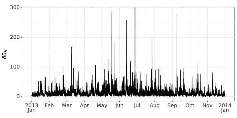
Figure 1: Raw $\delta B_{H}$ values for the Ottawa magnetometer.

To better account for the outliers seen in $\delta B_{H}$ prediction, we consider a GPR model with contaminated normal (CN) noise to account for outliers. This stands in contrast to other ML methods, particularly artificial neural networks (ANNs). Often, the estimates from ANN models result in poorly calibrated coverage intervals that are too wide for a given confidence level, especially during periods of solar storms when outliers become relatively routine. To combat this, we developed a contaminated-normal distribution for Gaussiaan Processes that accounts for changing variance over storm periods.

The CN distribution is a special case of a Gaussian mixture distribution with two components [4]. This distribution models outliers explicitly by assigning them to a mixture component with much larger variance. Therefore, the mixture proportions can be interpreted as the outlier and non-outlier proportion. Robust regression with mixture noise distributions is not a new concept. [5] first introduced a Bayesian linear regression model with mixture noise as a Bayesian approach to handling outliers. [6] follows up with a variational approximation for a similar model. Although the idea of modeling noise with mixture distributions in regression dates back to the 1960s, it is still being actively explored as a means to robustify modern statistical and machine learning methods. [7] proposed DeepGUM, a deep regression model with Gaussian-uniform mixture noise for performing various computer vision tasks in the presence of outliers. [8] developed the Mixture-of-Gaussian Lasso technique which models noise as a Gaussian mixture distribution in a sparse linear regression model. [9] introduced a probabilistic principal component regression model with switching Gaussian mixture noise for industrial process modeling.

GPR with mixture noise was first proposed by [10] who developed an expectation propagation (EP) algorithm and Markov chain Monte-Carlo (MCMC) sampling scheme for inference. [10] also developed inference algorithms for GPR models with Student-t and Laplace noise. Their experiments showed that the robust GPR models outperform the GPR model with Gaussian noise when outliers are present in the training data. However, predictive performance among the robust GPR models were similar for the simulated and real-world datasets they considered. [11] also considered a GPR model with mixture noise but used an EM algorithm for inference. [12] proposed the twinned GP model which also assumes a mixture noise distribution. However, they model the outlier proportion with another GP, effectively making their noise model heteroscedastic which is out of the scope of our proposed work. They showed that the twinned GP model is suitable in cases where outliers can be clustered. A major issue with the inference algorithms developed by [10], [11], and [12] is that they scale poorly with number of observations as they perform inference on exact GPs which require inverting a full kernel matrix.

In addition to GPR models with mixture noise, several other robust GPR methods have also been proposed. [13] provided a robust expectation propagation (EP) algorithm for GPR with student-t noise. [14] proposed iterative trimming for robust GPR. The main idea of their method is to iteratively trim a proportion of the observations with the largest absolute residuals so that they are not as influential to the resulting model fit. However, this may not be appropriate in cases where outliers are due to systematic effects not captured by the model but are still of interest to the analysis. [15] recently proposed using a Huber likelihood for robust GPR. This method employs weights based on projection statistics to scale residuals and bound the influence of outliers on the latent function estimate. Unfortunately, all of these methods also perform exact inference.

Many approximation methods for scaling up GPR to accomodate massive datasets have been proposed [16]. These approximation methods can be categorized as either global or local approximations. Global approximations approximate the kernel matrix, and as a result the latent function posterior, through global distillation. This can be achieved by computing the kernel matrix on only a subset of the training data, sparsifying the kernel matrix, or constructing a sparse approximation of the latent function posterior using a small number of inducing (or pseudo) points. Local approximations take a divide and conquer approach by focusing on local subsets of training data. While global approximations are better at capturing global patterns, they often filter out local patterns due to the use of inducing points. On the other hand, local approximations are better at capturing non-stationary features but risk local over-fitting. [16] provides a comprehensive review of both global and local approximation methods for GPR.

Sparse approximations have perhaps received the most attention in the GP community. Early work in this area involved approximating the GP prior with inducing points and then optimizing the marginal likelihood of the approximate model [17]. This includes the deterministic training conditional (DTC), fully independent training conditional (FITC), and partially independent training conditional (PITC) approximations which only differ in how they specify the dependency between the latent function and inducing points [18, 19, 20]. [21] further extended these approximated GP priors to be more flexible by placing the inducing points in a different domain via integral transforms. However, these approaches effectively alter the original model assumptions and may be prone to overfitting. This motivated the development of approximate inference approaches that make all the necessary approximations at inference time.

[22] first introduced the sparse variational GP (SVGP) method. A subtle but important distinction between this approach and earlier approaches is that the inducing points are now considered variational parameters and are decoupled from the original model. [22] jointly estimates the inducing points and model hyperparameters by maximizing a lower bound to the exact marginal likelihood as opposed to maximizing an approximate marginal likelihood. [23] extended this idea by reformulating the lower bound to enable stochastic optimization. [24] further modified this lower bound to accomodate non-Gaussian likelihoods and applied it to GP classification. Sparse variational methods are discussed in more detail in section 2.2. In this paper, we propose a scalable inference algorithm based on the SVGP method for fitting sparse GPR models with contaminated normal (CN) noise on large datasets.

The rest of the paper is organized as follows. Section 2 provides background on Gaussian process regression and sparse variational GPs. We then discuss our proposed model in section 3.1 followed by a corresponding inference algorithm in section 3.2. In section 4.1, we perform a simulation study to show the efficacy of our proposed inference algorithm. In section 4.2, we compare sparse GPR models with different noise distributions (CN, Gaussian, Student-t, Laplace) trained on simulated datasets. In section 4, we train sparse GPR models with different noise distributions on flight delays and ground magnetic perturbations data and compare their predictive performance. We conclude the paper with a brief summary and discussion on potential extensions in section 6. For all simulation studies and real-world data applications, we use the GPyTorch Python package to train GPR models [25].

2 Background

In this section, we provide a primer on Gaussian process regression and review sparse variational GPs.

2.1 Gaussian process regression

A Gaussian process (GP) is mathematically defined as a collection of random variables $\{f(\textbf{x})|\textbf{x}\in\mathcal{X}\}$, for some index set $\mathcal{X}$, for which any finite subset follows a joint Gaussian distribution. A GP is completely specified by its mean and covariance (or kernel) function defined by

$$m(\textbf{x}) =E[f(\textbf{x})],$$

$$k(\textbf{x},\textbf{x}^{\prime}) =E[(f(\textbf{x})-m(\textbf{x}))(f(\textbf{x}^{\prime})-m(\textbf{x}^{\prime}))].$$

GPs are commonly used as priors over real-valued functions. For the remainder of this paper, we will assume that $\mathcal{X}=\mathbb{R}^{d}$ and $m(\textbf{x})=0$. Suppose we have a training dataset consisting of inputs $\mathbf{X}=\{\textbf{x}_{i}\}_{i=1}^{n}$ and outputs $\mathbf{y}=\{y_{i}\}_{i=1}^{n}$. GP regression assumes that the outputs are noisy realizations of a latent function $f$ evaluated at the inputs, i.e. $y_{i}=f(\textbf{x}_{i})+\epsilon_{i}$, where $\epsilon_{i}$ is a noise term. Furthermore, we assume that $\mathbf{f}=\{f(\mathbf{x}_{i})\}_{i=1}^{n}$ follows a Gaussian process prior, i.e.

$$p(\mathbf{f}|\vartheta)=N(\mathbf{f}|\mathbf{0},\mathbf{K}_{nn}),$$ (1)

where $\mathbf{K}_{nn}=\{k(\textbf{x}_{i},\textbf{x}_{j};\vartheta)\}_{1\leq i,j\leq n}\in\mathbb{R}^{n\times n}$ is a covariance matrix with kernel hyperparameters $\vartheta$. For the rest of this paper, we will denote the Gaussian density with mean $\mu$ and variance $\sigma^{2}$ as $N(\cdot|\mu,\sigma^{2})$. We will drop the dependence on $\vartheta$ in our notation when it does not need to be emphasized. Combined with a likelihood function $p(\textbf{y}|\textbf{f})$, or equivalently a distribution for the noise term, the joint distribution between outputs and latent function values fully specifies the GPR model and takes the form

$$p(\mathbf{y},\mathbf{f})=p(\mathbf{y}|\mathbf{f})p(\mathbf{f}).$$ (2)

Note that this distribution and subsequent distributions will depend on inputs X and potential model/kernel hyperparameters but we will omit them in our notation whenever this dependence does not need to be emphasized. The likelihood is usually assumed to follow a Gaussian distribution with homoskedastic noise centered at f, i.e.

$$p(\textbf{y}|\textbf{f})=N(\mathbf{y}|\textbf{f},\sigma^{2}\mathbf{I}_{n})=\prod_{i=1}^{n}p(y_{i}|f(\mathbf{x}_{i}),\sigma^{2}),$$ (3)

where $\mathbf{I}_{n}$ denotes the $n\times n$ identity matrix. In section 3, we will replace this with a CN distribution to account for outliers or extreme observations. From the joint probability model specified by eq. 2, we can derive several distributions of interest, namely the marginal likelihood and posterior predictive distribution. These distributions can be derived in closed form if we make the Gaussian noise assumption in eq. 3. Marginalizing out f in eq. 2, we get that the marginal likelihood is given by

$$p(\textbf{y})=N(\textbf{y}|\mathbf{0},\mathbf{K}_{nn}+\sigma^{2}\mathbf{I}_{n}).$$ (4)

Maximum likelihood estimates of hyperparameters can be obtained by maximizing the marginal likelihood with respect to the hyperparameters using gradient-based optimization. The posterior process is also a GP with the following posterior mean and covariance functions:

$$m_{\mathbf{y}}(\mathbf{x}) =\mathbf{k}_{\mathbf{x}n}^{\prime}\tilde{\mathbf{K}}_{nn}^{-1}\mathbf{y},$$

$$k_{\mathbf{y}}(\mathbf{x},\mathbf{x}^{\prime}) =k(\mathbf{x},\mathbf{x}^{\prime})-\mathbf{k}_{\mathbf{x}n}^{\prime}\tilde{\mathbf{K}}_{nn}^{-1}\mathbf{k}_{\mathbf{x}^{\prime}n},$$

where $\mathbf{k}_{\mathbf{x}n}=\big{(}k(\mathbf{x},\mathbf{x}_{1}),\dots,k(\mathbf{x},\mathbf{x}_{n})\big{)}^{\prime}$ and $\tilde{\mathbf{K}}_{nn}=\mathbf{K}_{nn}+\sigma^{2}\mathbf{I}_{n}$. In other words, $p\big{(}f(\mathbf{x})|\mathbf{y}\big{)}=N\big{(}f(\mathbf{x})\big{|}m_{\mathbf{y}}(\mathbf{x}),k_{\mathbf{y}}(\mathbf{x},\mathbf{x})\big{)}$ for any $\mathbf{x}\in\mathbb{R}^{d}$. After obtaining hyperparameter estimates, we can make predictions at a test input $\mathbf{x}^{*}$ using the posterior predictive distribution:

$$p(y^{*}|\mathbf{y},\mathbf{x}^{*}) =\int p(y^{*}|f^{*})p(f^{*}|\mathbf{y})df^{*}$$

$$=N(y^{*}|m_{\mathbf{y}}(\mathbf{x}^{*}),\sigma^{2}+k_{\mathbf{y}}(\mathbf{x}^{*},\mathbf{x}^{*})).$$ (5)

A more comprehensive review of Gaussian process regression can be found in [26]. Computing eq. 5 involves inverting the $n\times n$ matrix $\tilde{\mathbf{K}}_{nn}$ which requires $O(n^{3})$ computations. This restricts the use of exact GPR models to datasets with up to a few thousand observations. Sparse approximations can be used to make GPR more scalable. Sparse GP methods approximate the latent function posterior by conditioning on a small number $m<<n$ of inducing points that act as a representative proxy for the observed outputs. These inducing points can either be chosen as a subset of the training data or optimized over. In the remainder of this section, we will discuss popular methods for jointly estimating the inducing points and hyperparameters.

Let $\mathbf{Z}=\{\mathbf{z}_{i}\}_{i=1}^{m}$ denote a set of inducing inputs, which may not be identical to the original inputs, and define the corresponding inducing points as $\mathbf{u}=\{f(\mathbf{z}_{i})\}_{i=1}^{m}$. It follows that $p(\textbf{u})=N(\textbf{u}|\mathbf{0},\mathbf{K}_{mm})$, where $\mathbf{K}_{mm}$ is defined analogously to $\mathbf{K}_{nn}$. The joint distribution between $\mathbf{f}$ and $\mathbf{u}$ is given by $p(\textbf{f},\textbf{u})=p(\textbf{f}|\textbf{u})p(\textbf{u}),$ where

$$p(\textbf{f}|\textbf{u})=N(\textbf{f}|K_{nm}\mathbf{K}_{mm}^{-1}\textbf{u},\mathbf{K}_{nn}-\mathbf{Q}_{nn}),$$ (6)

with $\mathbf{Q}_{nn}=\mathbf{K}_{nm}\mathbf{K}_{mm}^{-1}\mathbf{K}_{nm}^{\prime}$ and $\mathbf{K}_{nm}=\{k(\textbf{x}_{i},\textbf{z}_{j})\}\in\mathbb{R}^{n\times m}$. The original joint probability model in eq. 2 can then be augmented with the inducing points to form the model

$$p(\mathbf{y},\mathbf{f},\mathbf{u})=p(\mathbf{y}|\mathbf{f})p(\mathbf{f}|\mathbf{u})p(\mathbf{u}).$$ (7)

Note that integrating out $\mathbf{u}$ returns us to the original model so they are equivalent in terms of performing inference. However, inference with this augmented model still requires inverting $n\times n$ matrices. Several methods have been proposed to approximate the distribution in eq. 6, thereby modifying the GP prior and likelihood [17]. The fully independent training conditional (FITC) approximation removes the conditional dependencies between different elements in $\mathbf{f}$, i.e.

$$q(\mathbf{f}|\mathbf{u})=N\big{(}\mathbf{f}|\mathbf{K}_{nm}\mathbf{K}_{mm}^{-1}\mathbf{u},\text{diag}(\mathbf{K}_{nn}-\mathbf{Q}_{nn})\big{)},$$ (8)

where $\text{diag}(\mathbf{A})$ denotes a diagonal matrix formed with the diagonal elements of $\mathbf{A}$. This results in the following modified marginal likelihood:

$$\tilde{p}(\mathbf{y}|\mathbf{f})=N(\mathbf{y}|0,\sigma^{2}\mathbf{I}_{n}+\tilde{\mathbf{Q}}_{nn}),$$

where $\tilde{\mathbf{Q}}_{nn}=\mathbf{Q}_{nn}+\text{diag}(\mathbf{K}_{nn}-\mathbf{Q}_{nn})$ is an approximation to the true covariance $\mathbf{K}_{nn}$. Similarly, the deterministic training conditional (DTC) and partially independent training conditional (PITC) methods approximate $\mathbf{K}_{nn}$ with $\mathbf{Q}_{nn}$ and a block diagonalization of $\mathbf{K}_{nn}-\mathbf{Q}_{nn}$, respectively. The inducing points and hyperparameters can then be jointly estimated by maximizing the marginal log likelihood. With these approximations, the cost of inference and prediction is reduced from $O(n^{3})$ to $O(nm^{2})$. However, these methods are philosophically troubling as they entangle assumptions about the data embedded in the original likelihood with the approximations required to perform inference. Furthermore, $m$ new model parameters are added which increases the risk of overfitting. The sparse variational GP (SVGP) method, first introduced by [22], takes a different approach by approximating the exact posterior GP with variational inference. Before discussing this approach, we take a detour to give the reader a primer on variational inference.

2.2 Sparse variational GPs (SVGP)

In contrast to the DTC, FITC, and PITC approximations, the SVGP method performs inference with the exact augmented model in eq. 7 and approximates the posterior distribution $p(\mathbf{f},\mathbf{u}|\mathbf{y})=p(\mathbf{f}|\mathbf{u},\mathbf{y})p(\mathbf{u}|\mathbf{y})$ using variational inference. Appendix A provides a brief introduction to variational inference. In other words, we want to solve the following optimization problem:

$$q^{*}(\mathbf{f},\mathbf{u})=\underset{q}{\text{arg min }}\text{KL}\big{[}q(\mathbf{f},\mathbf{u})||p(\mathbf{f},\mathbf{u}|\mathbf{y})\big{]}.$$

To ensure efficient computation, the approximate posterior is assumed to factorize as

$$q(\mathbf{f},\mathbf{u})=p(\mathbf{f}|\mathbf{u})q(\mathbf{u}),$$ (9)

where $p(\mathbf{f}|\mathbf{u})$ is given in eq. 6; and $q(\mathbf{u})$ is a variational distribution for $\mathbf{u}$. To see why, let’s compute the ELBO from eq. 29:

$$\text{ELBO}=E_{q(\mathbf{f},\mathbf{u})}\Big{[}\log\frac{p(\mathbf{y}|\mathbf{f})p(\mathbf{f}|\mathbf{u})p(\mathbf{u})}{q(\mathbf{f},\mathbf{u})}\Big{]}.$$

If we assume $q(\mathbf{f},\mathbf{u})$ takes the form in eq. 9, then the $p(\mathbf{f}|\mathbf{u})$ terms in the log cancel out and the ELBO can be computed as

ELBO $$=E_{p(\mathbf{f}|\mathbf{u})q(\mathbf{u})}\Big{[}\log\frac{p(\mathbf{y}|\mathbf{f})p(\mathbf{u})}{q(\mathbf{u})}\Big{]}$$ (10)

$$=E_{q(\mathbf{u})}\Big{[}E_{p(\mathbf{f}|\mathbf{u})}[\log p(\mathbf{y}|\mathbf{f})]+\log\frac{p(\mathbf{u})}{q(\mathbf{u})}\Big{]}$$

$$=E_{q(\mathbf{f})}[\log p(\mathbf{y}|\mathbf{f})]-\text{KL}[q(\mathbf{u})||p(\mathbf{u})]$$

$$=\sum_{i=1}^{n}E_{q(f_{i})}[\log p(y_{i}|f_{i})]-\text{KL}[q(\mathbf{u})||p(\mathbf{u})]=\mathcal{L}_{\text{svgp}},$$ (11)

where $f_{i}=f(\textbf{x}_{i})$ and $q(\mathbf{f})=\int p(\mathbf{f}|\mathbf{u})p(\mathbf{u})d\mathbf{u}$. This can be computed with $O(nm^{2})$ computations. [22] showed that under a Gaussian likelihood, this ELBO can be maximized without explicitly computing the optimal $q(\mathbf{u})$ by maximizing the lower bound:

$$\log N(\mathbf{y}|0,\sigma^{2}\mathbf{I}+\mathbf{Q}_{nn})-\frac{1}{2\sigma^{2}}\text{Tr}(\tilde{\mathbf{K}}_{nn}),$$

where $\tilde{\mathbf{K}}_{nn}=\mathbf{K}_{nn}-\mathbf{Q}_{nn}$; and $\text{Tr}(\mathbf{A})$ denotes the trace of matrix $\mathbf{A}$. The derivation for this lower bound is given in appendix B. In order to maximize the ELBO using stochastic variational inference, [23] proposed maintaining an explicit variational distribution given by

$$q(\mathbf{u})=N(\mathbf{u}|\mathbf{m},\mathbf{S}).$$ (12)

This yields the following form for $q(\mathbf{f})$:

$$q(\mathbf{f})=N(\mathbf{f}|\mathbf{A}\mathbf{m},\mathbf{K}_{nn}+\mathbf{A}(\mathbf{S}-\mathbf{K}_{mm})\mathbf{A}^{\prime}),$$ (13)

where $\mathbf{A}=\mathbf{K}_{nm}\mathbf{K}_{mm}^{-1}$. Under a Gaussian likelihood, the ELBO becomes

$$\sum_{i=1}^{n}\Big{[}\log N(y_{i}|\mathbf{k}_{i}^{\prime}\mathbf{K}_{mm}^{-1}\mathbf{m},\sigma^{2})-\frac{1}{2}\sigma^{-2}\tilde{\mathbf{k}}_{ii}-\frac{1}{2}\text{Tr}(\mathbf{S}\mathbf{\Lambda}_{i})\Big{]}-\text{KL}[q(\mathbf{u})||p(\mathbf{u})],$$

where $\mathbf{k}_{i}$ is the $i$th column of $\mathbf{K}_{mn}$; $\tilde{\mathbf{k}}_{ii}$ is the $i$th diagonal element of $\tilde{\mathbf{K}}_{nn}$; and $\mathbf{\Lambda}_{i}=\sigma^{-2}\mathbf{K}_{mm}^{-1}\mathbf{k}_{i}\mathbf{k}_{i}^{\prime}\mathbf{K}_{mm}^{-1}$ (Section 3.1 of [23]). Furthermore, the approximate predictive distribution at a new input $\mathbf{x}^{*}$ is given by

$$q_{\text{pred}}(y^{*}|\mathbf{x}^{*}) =\int p(y^{*}|\mathbf{f}^{*})q(\mathbf{f}^{*})d\mathbf{f}^{*}$$

$$=N(y^{*}|\mu_{f^{*}},\sigma_{f^{*}}^{2}+\sigma^{2}),$$ (14)

where $\mu_{f^{*}}=k_{*}^{\prime}\mathbf{K}_{mm}^{-1}\mathbf{m}$, $\sigma_{f^{*}}^{2}=k(\mathbf{x}^{*},\mathbf{x}^{*})+\mathbf{k}_{*}^{\prime}\mathbf{A}\mathbf{k}_{*}$, and $\mathbf{k}_{*}=\{k(\mathbf{x}^{*},\mathbf{x}_{i})\}_{i=1}^{n}$. $\mathcal{L}_{\text{svgp}}$ can be computed for non-Gaussian likelihoods as long as the expectation in eq. 11 can be computed or approximated. Inference with SVGP involves maximizing $\mathcal{L}_{\text{svgp}}$ with respect to variational, likelihood, and kernel hyperparameters. In section 3.2, we show how this method can be extended to perform inference in GPR with CN noise.

3 Methods

3.1 Model specification

We propose to replace the Gaussian noise assumption made in eq. 3 with the following contaminated normal (CN) noise assumption:

$$p(y_{i}|f_{i})=\pi N(y_{i}|f_{i},\tau\sigma^{2})+(1-\pi)N(y_{i}|f_{i},\sigma^{2}),\ \ i=1,\dots,n,$$ (15)

where $\sigma^{2}>0$ is the noise variance for non-outlier observations; $\tau>1$ is an inflation parameter which represents the increased variance due to outliers; and $0<\pi<1$ gives the proportion of outliers. In contrast to other robust likelihoods such as the Laplace or Student-t likelihood, this likelihood explicitly models the outliers by giving them an outsized variance compared to non-outlier or extreme observations. This is motivated by the needs of modeling occasional extreme phenomena in geomagnetic disturbances as shown in Figure 1 in the Introduction.

3.2 Inference

Let $\theta=(\pi,\tau,\sigma^{2})$ denote our model hyperparameters. A naive approach to estimating $\theta$ is to directly plug eq. 15 into $\mathcal{L}_{\text{svgp}}$ in eq. 11 and maximize it with respect to $\theta$ using gradient-based optimization. However, the expectation term in eq. 11 would not have a closed form and would need to be approximated. In this section, we derive a modified ELBO based on eq. 11 for our proposed model and introduce a stochastic generalized alternating maximization (SGAM) algorithm to maximize it in order to estimate $\theta$ and other hyperparameters. We begin by introducing a set of binary latent variables $\{\alpha_{i}\}_{i=1}^{n}$ that represent the component assignments for each observation, i.e.

$$p(\alpha_{i}=1|\theta)=\pi,\quad p(y_{i}|f_{i},\alpha_{i},\theta)=N(y_{i}|f_{i},\tau^{\alpha_{i}}\sigma^{2}).$$ (16)

Following the same logic in appendix A, the log likelihood function $\log p(y_{i}|f_{i},\theta)$ can be decomposed as

$$\log p(y_{i}|f_{i},\theta)=F(q(\alpha_{i}|f_{i}),\theta)+\text{KL}\big{[}q(\alpha_{i}|f_{i})||p(\alpha_{i}|y_{i},f_{i},\theta)\big{]},$$

for any distribution $q(\alpha_{i}|f_{i})$, where

$$F(q(\alpha_{i}|f_{i}),\theta) =E_{q(\alpha_{i}|f_{i})}\Big{[}\log\Big{(}\frac{p(y_{i},\alpha_{i}|f_{i},\theta)}{q(\alpha_{i}|f_{i})}\Big{)}\Big{]}$$

$$=E_{q(\alpha_{i}|f_{i})}[\log p(y_{i},\alpha_{i}|f_{i},\theta)]+H(q(\alpha_{i}|f_{i}));$$

and $H(p(x))=-\int p(x)\log p(x)dx$ is the entropy function. Since the KL divergence is non-negative, $F(q(\alpha_{i}|f_{i}),\theta)$ provides a lower bound for the log likelihood function. By extension of eq. 11, this gives us the following modified ELBO:

$$\log p(\mathbf{y}|\Theta) \geq\sum_{i=1}^{n}E_{q(f_{i},\alpha_{i}|\varphi,\vartheta)}\big{[}F(q(\alpha_{i}|f_{i}),\theta)\big{]}-\text{KL}[q(\mathbf{u})||p(\mathbf{u});\vartheta]$$

$$=\sum_{i=1}^{n}\Big{\{}E_{q(f_{i},\alpha_{i}|\varphi,\vartheta)}\big{[}\log p(y_{i},\alpha_{i}|f_{i},\theta)\big{]}+$$ (17)

$$E_{q(f_{i}|\varphi,\vartheta)}\big{[}H(q(\alpha_{i}|f_{i}))\big{]}\Big{\}}-\text{KL}[q(\mathbf{u})||p(\mathbf{u});\vartheta]$$

$$=\mathcal{L}(q,\Theta),$$ (18)

where $\Theta=(\theta,\vartheta)$ denotes the model and kernel hyperparameters and $q(f_{i},\alpha_{i}|\varphi,\vartheta)=q(\alpha_{i}|f_{i})q(f_{i}|\varphi,\vartheta)$. We assume $q(f_{i}|\varphi,\vartheta)$ is the Gaussian variational distribution given in eq. 13. Although the true latent function posterior may have multiple modes in this case, [10] showed that a Laplace approximation for the latent function posterior of an exact GP with mixture noise works reasonably well in the presence of a few outliers. Since $q(\textbf{u})$ and $p(\textbf{u})$ are both Gaussian, the KL divergence term can be expressed as a sum of $n$ terms and therefore, $\mathcal{L}(q,\Theta)$ can be written as $\mathcal{L}(q,\Theta)=\sum_{i=1}^{n}\mathcal{L}_{i}(q,\Theta)$. This allows it to be maximized using stochastic optimization methods. For the rest of this section, we describe the SGAM algorithm for maximizing the modified ELBO (or equivalently, minimizing the negative modified ELBO).

Let $\Theta^{(0)}=(\theta^{(0)},\vartheta^{(0)})$ denote the starting hyperparameter values. Furthermore, let $q^{(0)}(f_{i},\alpha_{i})=q(\alpha_{i}|f_{i})q(f_{i}|\varphi^{(0)},\vartheta^{(0)})$ denote the starting variational distribution with hyperparameters $\varphi^{(0)}$. At each iteration $t\geq 1$, the SGAM algorithm alternates between a forward and backward step. Let $I_{t}$ be a random subset uniformly sampled from $\{1,\dots,n\}$. In the forward step, we update $q(f_{i},\alpha_{i})$, with $\Theta=\Theta^{(t-1)}$, by first updating $q(\alpha_{i}|f_{i})$ with

$$q^{(t)}(\alpha_{i}|f_{i})=p(\alpha_{i}|f_{i},y_{i},\Theta^{(t-1)}).$$

This is equivalent to the E-step update in the standard EM algorithm where $f_{i}$ is held fixed. Furthermore, it maximizes $\mathcal{L}(q,\Theta^{(t-1)})$ with respect to $q(\alpha_{i}|f_{i})$. Next, we obtain $\varphi^{(t)}$ by taking a stochastic gradient descent (SGD) step with respect to $\varphi$, i.e.

$$\varphi^{(t)}\leftarrow\varphi^{(t-1)}+\alpha_{1}^{(t)}\nabla_{\varphi}\mathcal{L}_{I_{t}}(\tilde{q}_{\varphi}^{(t)},\Theta^{(t-1)}),$$ (19)

where $\tilde{q}_{\varphi}^{(t)}(f_{i},\alpha_{i})=q^{(t)}(\alpha_{i}|f_{i})q(f_{i}|\varphi,\vartheta^{(t-1)})$; $\alpha^{(t)}_{1}$ denotes the learning rate at iteration $t$; $\mathcal{L}_{I_{t}}=\sum_{i\in I_{t}}\mathcal{L}_{i}$; and $\nabla_{\varphi}$ denotes the gradient operator with respect to $\varphi$. The resulting forward step update is given by

$$q^{(t)}(f_{i},\alpha_{i})=q(f_{i}|\varphi^{(t)},\vartheta^{(t-1)})p(\alpha_{i}|f_{i},y_{i},\Theta^{(t-1)}).$$

In the backward step, we update $\Theta$ by first maximizing

$$\mathcal{L}(q^{(t)},\Theta)=\rm{const.}+\sum_{i=1}^{n} -\frac{1}{2}\Big{[}\log(\sigma^{2})+\hat{\alpha}_{i}^{(t)}\log(\tau)+$$

$$\sigma^{-2}\big{(}1+(\tau^{-1}-1)\hat{\alpha}_{i}^{(t)}\big{)}D_{i}^{(t)}\Big{]}$$

$$+\hat{\alpha}_{i}^{(t)}\log(\pi)+(1-\hat{\alpha}_{i}^{(t)})\log(1-\pi)$$ (20)

with respect to $\theta$, where

$$\hat{\alpha}_{i}^{(t)} =\int p(\alpha_{i}=1|f_{i},y_{i},\Theta^{(t-1)})q(f_{i}|\varphi^{(t)},\vartheta^{(t-1)})df_{i}$$

$$=\frac{\pi^{(t-1)}\Psi_{i}^{(t)}\big{(}\tau^{(t-1)}\sigma^{2(t-1)}\big{)}}{\pi^{(t-1)}\Psi_{i}^{(t)}\big{(}\tau^{(t-1)}\sigma^{2(t-1)}\big{)}+(1-\pi^{(t-1)})\Psi_{i}^{(t)}\big{(}\sigma^{2(t-1)}\big{)}},$$

with $D_{i}^{(t)}=E_{q^{(t)}(f_{i})}\big{[}(y_{i}-f_{i})^{2}\big{]}=(y_{i}-\mu_{f_{i}}^{(t)})^{2}+\sigma_{f_{i}}^{2(t)}$ and $\Psi_{i}^{(t)}(x)=N(y_{i}|\mu_{f_{i}}^{(t)},\sigma_{f_{i}}^{(t)}+x)$. It can be shown that the following closed-form updates maximize eq. 20:

$$\pi^{(t)} =\frac{N_{i}^{(t)}}{n},$$

$$\sigma^{2(t)} =\frac{1}{n}\sum_{i=1}^{n}\Big{(}1+\big{(}(\tau^{(t-1)})^{-1}-1\big{)}\hat{\alpha}_{i}^{(t)}\Big{)}D_{i}^{(t)},$$

$$\tau^{(t)} =\frac{1}{\sigma^{2(t)}N_{i}^{(t)}}\sum_{i=1}^{n}\hat{\alpha}_{i}^{(t)}D_{i}^{(t)},$$ (21)

where $N_{i}^{(t)}=\sum_{i=1}^{n}\hat{\alpha}_{i}^{(t)}$. Similar to the forward step, the second part of the backward step involves taking a SGD step with respect to $\vartheta$, i.e.

$$\vartheta^{(t)}\leftarrow\vartheta^{(t-1)}+\alpha_{2}^{(t)}\nabla_{\vartheta}\mathcal{L}_{I_{t}}(q^{(t)},\tilde{\Theta}^{(t)}),$$

where $\tilde{\Theta}^{(t)}=(\theta^{(t)},\vartheta)$; and $\alpha_{2}^{(t)}$ is the learning rate at iteration $t$. To make this more computationally efficient, we can also take a SGD step with respect to $\theta$ to obtain $\theta^{(t)}$ instead of computing the closed-form updates in the first part of the backward step. Note that the $\tau^{(t)}$ update in eq. 21 is not constrained to be greater than 1. If the final $\tau$ estimate is less than 1, we can replace $\sigma^{2}$ with $\tau\sigma^{2}$, $\tau$ with $\tau^{-1}$, and $\pi$ with $1-\pi$ so that $\tau$ and $\pi$ can still be interpreted as the variance inflation parameter and outlier probability, respectively. The approximate posterior predictive distribution at a new input $\mathbf{x}^{*}$ is given by

$$q_{\text{pred}}(y^{*}|\mathbf{y},\mathbf{x}^{*})=\pi N(y^{*}|\mu_{f^{*}},\sigma_{f^{*}}^{2}+\tau\sigma^{2})+(1-\pi)N(y^{*}|\mu_{f^{*}},\sigma^{2}),$$ (22)

where $\mu_{f^{*}}$ and $\sigma_{f^{*}}^{2}$ are the same as in eq. 14.

4 Simulation Studies

In this section, we perform several simulation studies to evaluate the performance of our proposed method and to compare it to similar methods. In the first simulation study, we show that our proposed algorithm is able to recover ground truth parameter and latent function values. In the second simulation study, we compare sparse variational GPR models with Gaussian (GPR-G), contaminated normal (GPR-CN), Student-t (GPR-t), and Laplace (GPR-L) distributed noise on simulated data with varying degrees of outlierness. We show that GPR-CN outperforms the other considered methods when there is a non-negligible proportion of outliers. We evaluate the four methods using the root mean squared error (RMSE), mean absolute error (MAE), and negative log predictive density (NLPD) metrics. We use the RMSE and MAE to evaluate the predictive mean functions. To evaluate the predictive distribution, we use the NLPD metric. The RMSE between observed values $\mathbf{y}$ and predicted values $\hat{\mathbf{y}}$ is defined as

$$\text{RMSE}(\mathbf{y},\hat{\mathbf{y}})=\sqrt{\frac{1}{n}\sum_{i=1}^{n}(y_{i}-\hat{y}_{i})^{2}}.$$

The MAE between $\mathbf{y}$ and $\hat{\mathbf{y}}$ is defined as

$$\text{MAE}(\mathbf{y},\hat{\mathbf{y}})=\frac{1}{n}\sum_{i=1}^{n}|y_{i}-\hat{y}_{i}|.$$

The NLPD is defined as the average negative log value of the predictive distribution at test inputs $\mathbf{X}^{*}$ with test outputs $\mathbf{y}^{*}$:

$$\text{NLPD}(\mathbf{y}^{*})=-\frac{1}{n}\sum_{i=1}^{n}\log p_{\text{pred}}(y_{i}^{*}|\mathbf{x}_{i}^{*}).$$

This measure is commonly used to compare predictive performance on unseen data among different models [27]. For GPR-G and GPR-CN, $p_{\text{pred}}$ is given in eq. 14 and eq. 22, respectively. For GPR-t and GPR-L, $\log p_{\text{pred}}$ is approximated using Monte-Carlo methods, i.e.

$$\log p_{\text{pred}}(y^{*}|\mathbf{x}^{*})\approx\frac{1}{M}\sum_{m=1}^{M}\log p(y^{*}|f^{(m)},\vartheta),\ \ f^{(m)}\sim q(f^{(m)}|\mathbf{X}^{*},\varphi),$$

where $M$ is the number of Monte-Carlo samples; $q$ is the variational distribution given in eq. 13; and $\log p(y^{*}|f^{(m)},\vartheta)$ is the log-likelihood function for either the Student-t or Laplace distribution centered at $f^{(m)}$ with hyperparameters $\vartheta$. We set $M=1000$ when computing the NLPD for GPR-t and GPR-L. Furthermore, the expectation term in eq. 11 for GPR-t and GPR-L are also intractable and are approximated using the Gauss-Hermite quadrature method [28]. In each of the simulations below, we use the popular squared exponential kernel with automatic relevance determination (ARD) defined as

$$k_{\text{se}}(\mathbf{x},\mathbf{x}^{\prime})=\sigma_{s}^{2}\exp\Bigg{(}-\sum_{j=1}^{p}\frac{||x_{j}-x_{j}^{\prime}||^{2}}{2\ell_{j}^{2}}\Bigg{)},\ \ \mathbf{x},\mathbf{x}^{\prime}\in\mathbb{R}^{p},$$ (23)

where $\sigma_{s}^{2}$ is an output scale parameter; and $\{\ell_{j}\}_{j=1}^{p}$ are individual length scales for each input dimension. We train each SVGPR model with 500 inducing points for 30 iterations using the Adam algorithm implemented in PyTorch with an exponentially decaying step size starting at 0.1 and a batch size of 256 [29, 30]. The inducing inputs were initialized to be a random sample of the training inputs. Since the objective function for GPR-CN and GPR-t may have multiple local optima, we rerun our algorithm five times with different initial parameter values and keep the run that yields the largest value for eq. 18 in each simulation study.

4.1 Parameter estimation

For the first simulation study, we simulate 200 datasets of size $n=5000$ directly from the model in eq. 15 with $\pi=0.1$, $\tau=10$, $\sigma^{2}=1$, and

$$f(x_{i})=0.3+0.4x_{i}+0.5\text{sin}(2.7x_{i})+\frac{1.1}{1+x_{i}^{2}},$$ (24)

where $x_{1},\dots,x_{5000}\sim\text{Uniform}(0,5)$. We plot one of the simulated datasets in fig. 2. This was adapted from an artificial regression problem considered by [31]. We plot the parameter estimates and corresponding ELBO value across iterations for one dataset in fig. 3. In this specific run, the parameter estimates converge to a value close to the true value after roughly 35 iterations. Figure 4 shows boxplots for estimated parameter values across the different simulated datasets. These boxplots show that most of the estimated values are close to the true parameter values. We plot the estimated mean functions and their respective RMSE values in fig. 5. From these plots, we can see that the estimated mean functions are close to the true function most of the time.

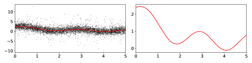
Figure 2: Simulated data for our first simulation study. The true function from eq. (24) is shown in red. Noisy observations are plotted on the left.

Figure 3: Parameter estimates and ELBO value across iterations for a specific run. Red dashed lines show the true parameter value.

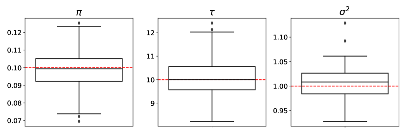
Figure 4: Boxplots for estimated parameter values from our proposed algorithm applied to 200 different simulated datasets. Red dashed lines show the true parameter value.

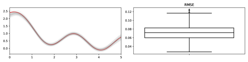
Figure 5: Function estimates from our proposed algorithm applied to 200 different simulated datasets. The true function from eq. (24) is shown in red. Estimated mean functions are shown in gray on the left. RMSEs for the estimated mean functions are given in the boxplot on the right.

4.2 Comparison with other robust likelihoods

For the second simulation study, we consider an artificial regression problem described in [10] which uses the following function first introduced in [32]:

$$f(\mathbf{x})=10\text{sin}(\pi x_{1}x_{2})+20(x_{3}-0.5)^{2}+10x_{4}+5x_{5},$$ (25)

where $\mathbf{x}=(x_{1},\dots,x_{10})$. The last 5 dimensions in $\mathbf{x}$ are ignored in order to incorporate feature selection to the problem. We generate $N_{\text{rep}}=200$ datasets of size $n=5000$ by sampling $\mathbf{x}_{1},\dots,\mathbf{x}_{5000}$ from the uniform distribution on the unit hyper-cube $[0,1]^{10}$. We then compute the corresponding function values in eq. 25 and add standard normal noise to it, i.e.

$$y_{i}=f(\mathbf{x}_{i})+\epsilon_{i},\ \ \epsilon_{i}\sim N(0,1).$$

Lastly, we add outliers by replacing $p_{\text{outlier}}$ proportion of the generated observations with samples drawn from $N(15,\sigma_{\text{outlier}}^{2})$, where $p_{\text{outlier}}\in\{0.1,0.2,0.3\}$ and $\sigma_{\text{outlier}}\in\{3,10\}$. In the $\sigma_{\text{outlier}}=3$ case, the generated outliers are likely to lie in the same range as the function values. Setting $\sigma_{\text{outlier}}=10$ constitutes a more difficult case where the outliers are unrelated to the function and are likely to lie outside of the function value range. We consider four scenarios with increasing outlier proportion and magnitude to study the performance of the considered noise models. These scenarios are summarized in table 1. The first scenario is the same one considered in [10] and serves as a baseline for the remaining scenarios which have an increasing proportion of extreme outliers. We fit the various GPR models to simulated datasets generated under various outlier scenarios and evaluate them on 10,000 noise-free test samples of eq. 25.

	$p_{\text{outlier}}$	$\sigma_{\text{outlier}}$	Description
1	0.1	3	Low proportion, mild outliers
2	0.1	10	Low proportion, extreme outliers
3	0.2	10	Medium proportion, extreme outliers
4	0.3	10	Large proportion, extreme outliers

Table 1: Summary of outlier scenarios considered in second simulation study.

Boxplots of the RMSE, MAE, and NLPD for the different models and outlier scenarios are given in figs. 6, 7, 8 and 9. Note that the boxplots for GPR-CN and GPR-t tend to have a higher spread compared to GPR-G and GPR-L. This is likely because these methods have ELBOs that are not log-concave and are vulnerable to local optima. Furthermore, the NLPDs for GPR-t are approximated with Monte-Carlo samples. In all scenarios, the robust noise models (GPR-CN, GPR-t, GPR-L) outperform GPR-G in terms of all metrics. The RMSEs and MAEs are similar for the robust noise models (GPR-CN, GPR-t, GPR-L) in all scenarios. In the first scenario, the NLPDs are similar for GPR-CN and GPR-t but are slightly higher for GPR-L. This difference in NLPDs is exacerbated in the remaining scenarios, where the outliers are more extreme. This is likely because the Laplace distribution is not as heavy-tailed as the t-distribution and does not model outliers separately as in the CN distribution. As we increase the proportion of outliers, GPR-CN starts to outperform GPR-t in terms of NLPD. This suggests that GPR-CN is more adept at handling larger proportions of outliers than GPR-t. This may be due to the fact that outliers are identified and placed into its own separate component in GPR-CN so they don’t affect model fit for non-outliers. On the other hand, outliers are not explicitly isolated in GPR-t so they may affect the fit for non-outliers. As the proportion of outliers increases, we may expect the true latent function posterior to be multimodal, making the Gaussian variational distribution inadequate for approximating it. However, this does not seem to hinder predictive performance as can be seen from the results in the third and fourth scenario.

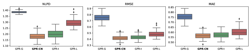
Figure 6: $p_{\text{outlier}}=0.1$, $\sigma_{\text{outlier}}=3$. Boxplots of NLPD, RMSE, and MAE for second simulation study with varying $p_{\text{outlier}}$ and $\sigma_{\text{outlier}}$ across 200 simulated datasets.

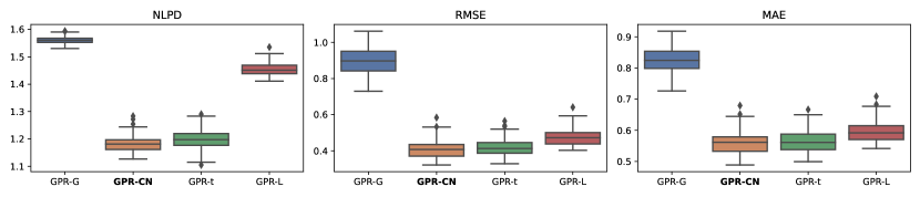
Figure 7: $p_{\text{outlier}}=0.1$, $\sigma_{\text{outlier}}=10$. Boxplots of NLPD, RMSE, and MAE for second simulation study with varying $p_{\text{outlier}}$ and $\sigma_{\text{outlier}}$ across 200 simulated datasets.

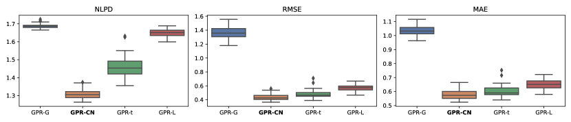
Figure 8: $p_{\text{outlier}}=0.2$, $\sigma_{\text{outlier}}=10$. Boxplots of NLPD, RMSE, and MAE for second simulation study with varying $p_{\text{outlier}}$ and $\sigma_{\text{outlier}}$ across 200 simulated datasets.

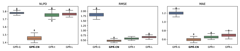
Figure 9: $p_{\text{outlier}}=0.3$, $\sigma_{\text{outlier}}=10$. Boxplots of NLPD, RMSE, and MAE for second simulation study with varying $p_{\text{outlier}}$ and $\sigma_{\text{outlier}}$ across 200 simulated datasets.

5 Applications

In this section, we fit the four SVGPR models identified in section 4.2 on flight delays. For ground magnetic perturbations data ($\delta B_{H}$), we fit a dense artificial neural network and a GPR-CN model and compare their predictive performances with skill scores, RMSE, and focus in depth on invterval coverage.

The model fitting procedure varies slightly between datasets. For the flights data, we train the four GPR models with 1000 inducing points for up to 30 iterations using the Adam algorithm implemented in PyTorch with an exponentially step size starting at 0.1 and a batch size of 256 [29, 30]. The inducing inputs were initialized to be a random sample of the training inputs. We used a validation set to monitor the validation NLPD and terminate training if it hasn’t decreased in 5 iterations. Input features are standardized by subtracting the training sample mean and dividing by the training sample standard deviation.

For $\delta B_{H}$ prediction, we use a more flexible hyperparameter setup, opting to allow the number of inducing points and batch size to vary and choosing optimal hyperparameters using the Bayesian Optimization package [33]. As the data is fully numeric and relatively small station by station, we use a large batch size on a GPU to speed up computation. The details of this can be found in 5.2.2.

For the flight delays data, we use the ARD squared exponential kernel defined in eq. 23. For the ground magnetic perturbations data, we use the ARD Matern kernel with smoothness parameter $\nu$ defined as

$$k_{\text{matern}}(\mathbf{x},\mathbf{x}^{\prime})=\sigma_{s}^{2}\frac{2^{1-\nu}}{\Gamma(\nu)}\big{(}\sqrt{2\nu}d\big{)}^{\nu}K_{\nu}\big{(}\sqrt{2\nu}d\big{)},\ \ \mathbf{x},\mathbf{x}^{\prime}\in\mathbb{R}^{p},$$

where $d=\sum_{j=1}^{p}\ell_{j}^{-2}||x_{j}-x_{j}^{\prime}||^{2}$; $K_{\nu}$ is the modified Bessel function; $\sigma_{s}^{2}$ is an output scale parameter; and $\{\ell_{j}\}_{j=1}^{p}$ are individual length scales for each input dimension. We set $\nu=1.5$ which allows us to rewrite $k_{\text{matern}}$ as

$$k_{\text{matern}}(\mathbf{x},\mathbf{x}^{\prime})=\sigma_{s}^{2}\big{(}1+\sqrt{3}d\big{)}\exp\big{(}-\sqrt{3}d\big{)}.$$

5.1 Flight delays

The flight delays dataset consists of information about commercial flights in the US from January 2008 to April 2008 and was taken from an example in [23]. It has become a standard benchmark dataset in the GPR literature for comparing scalable GPR methods due to its massive size and non-stationary nature. The original dataset curated by [23] contains 800,000 observations that were randomly sampled from a dataset containing around 2 million observations. To speed up computation, we reduced the size by randomly sampling 100,000 observations for training, and 20,000 each for validating and testing. The goal is to predict flight delay times (in minutes) using the eight features considered by [23]: aircraft age, distance to travel, airtime, departure time, arrival time, day of the week, day of the month, and month. A histogram of flight delay times used for training is given in fig. 10. 99% of flights are only delayed for up to 166 minutes. However, there are a handful of flights that are delayed for more than 300 minutes. These delays are likely due to external factors such as weather that are not considered in our models. This motivates the use of robust models for analyzing this data.

Min.	Q25	Median	Mean	Q75	Q99	Max
-81	-9	-1	9.4	13	166	637

Table 2: Summary statistics for flight delay times (in minutes) used for training.

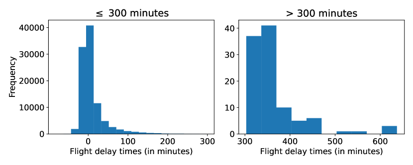
Figure 10: Histograms of flight delay times (in minutes) used for training. Left plot shows histogram for delays less than or equal to 300 minutes. Right plot shows histogram for delays greater than 300 minutes.

We fit the models considered in section 4.2 to this dataset and compare their predictive performances. For this dataset, we also use the ARD squared exponential kernel defined in eq. 23. The NLPD, RMSE, and MAE for the four GPR models fitted to this dataset are reported in table 3. GPR-CN has the lowest NLPD and ties with GPR-L for the lowest MAE. GPR-G has the lowest RMSE but highest MAE. This suggests that the resulting model fit for GPR-G is more heavily influenced by outliers than the ones for the other methods.

	NLPD	RMSE	MAE
GPR-G	4.95	34.38	4.65
GPR-CN	4.51	36.94	4.32
GPR-t	4.62	37.55	4.35
GPR-L	5.38	36.12	4.32

Table 3: Metrics for GPR models trained on flight delays data. The lowest value(s) in each column are shown in bold.

5.2 Ground magnetic perturbations

To determine the effectiveness of the GPR-CN on real world data, we turn our attention back to $\delta B_{H}$ prediction. This data differs from the flights dataset considerably; first, it is messier, and more prone to missingness and measurement error. We examine the results of applying the GPR-CN model to $\delta B_{H}$ prediction below.

5.2.1 Data Setup

For this project, we chose twelve test stations commonly used in the space weather literature.

For the FUR station, we were unable to produce a consistent GPR-CN fit, and so the results are reported for the remaining eleven. Due to missing data, the station PBQ is replaced by the nearby station T31/SNK (Sanikiluaq); the FRN station (Fresno) is replaced by the nearby station T16 (Carson City) for the year 2015.

Table 4: All test data. Summary statistics of GPR-CN and ANN models for the testing period of 2015-2016. Target coverage is 95%. Coverage is comparable in both storm and non-storm periods, but the IQR of interval length is generally either comparable or lower in the GPR-CN model.

	RMSE		Coverage		Interval Length (IQR)
Model	ANN	GPR-CN	ANN	GPR-CN	ANN	GPR-CN
Station
ABK	87.874	86.055	0.934	0.908	322.678	104.563
FRD	11.861	13.044	0.938	0.978	20.813	29.105
FRN	14.012	15.558	0.934	0.963	21.230	30.694
HRN	65.169	65.712	0.941	0.946	164.701	121.076
IQA	81.283	83.912	0.894	0.979	207.880	237.874
MEA	73.432	78.744	0.929	0.909	68.185	40.418
NEW	16.420	18.681	0.923	0.952	24.106	25.724
OTT	15.522	18.473	0.918	0.941	21.987	25.464
PBQ	85.699	92.237	0.934	0.913	171.892	108.511
WNG	13.923	15.007	0.925	0.941	23.780	23.911
YKC	93.764	96.636	0.948	0.951	287.425	208.491

Table 5: Storm periods only. Summary statistics of GPR-CN and ANN models for the testing period of 2015-2016. Target coverage is 95%. Coverage is comparable in both storm and non-storm periods, but the IQR of interval length is generally either comparable or lower in the GPR-CN model.

	RMSE		Coverage		Interval Length (IQR)
Model	ANN	GPR-CN	ANN	GPR-CN	ANN	GPR-CN
Station
ABK	145.126	118.050	0.939	0.905	891.077	167.798
FRD	25.133	31.673	0.883	0.964	41.961	47.423
FRN	33.742	36.837	0.840	0.890	44.144	46.963
HRN	104.870	106.009	0.878	0.901	333.435	204.989
IQA	109.992	128.926	0.966	0.951	320.797	295.607
MEA	114.532	132.416	0.933	0.870	148.557	68.892
NEW	33.443	41.519	0.921	0.931	43.032	45.698
OTT	40.779	55.719	0.846	0.863	36.850	40.187
PBQ	113.425	129.959	0.933	0.901	296.378	189.384
WNG	29.586	35.025	0.885	0.893	38.889	37.622
YKC	144.834	158.726	0.950	0.942	482.269	319.620

For each of these twenty minute intervals, we use lagged OMNI data as our primary input features. The OMNI data is collected every minute, but we use the median value for every five minutes over the previous hour as our input features. After this, we compute seasonal features for both time of day and the day of the year. This gives us a total of ninety-six input features with which to predict $\delta B_{H}$ for each station.

Following the convention made in the space weather community, we do not include prior values of the output as inputs [34, 35, 36]. Therefore, we will ignore the temporal nature of this data and treat it as a conventional regression problem. Space physicists are typically most interested in the predictive performance during geomagnetic storms when $\delta B_{H}$ spikes, and so we report results across the entire prediction range as well as within storm performance.

The SuperMAG data is stored in Parquet files divided by station. The data are loaded from these files and any missing points are dropped; as our approach is to use covariates only and not any lagged SuperMAG data, gaps in the response variable do not significantly affect the model fit. Once we have a SuperMAG series with no missing entries, relevant OMNI features are matched by timestamp to the SuperMAG series.

5.2.2 Models

To fit the models, we divided the data into three time periods. Training consists of the twenty minute maximum $\delta B_{H}$ value from 2010-2013. We held out 2014 and 2015 as validation and testing sets, respectively. Model fits are performed independently by station. In addition to the GPR-CN model, we fit a dense ANN to serve as a performance baseline.

In the context of ANN model, deriving a probabilistic interpretation of uncertainties and contrasting this with GPR methods poses a unique challenge. To facilitate inference within our predictions, we assume that each data point follows a normal distribution, and we employ a 4-layer deep multi-output neural network designed to estimate both location parameters $\hat{\mu}$ and scale parameters $\hat{\sigma}^{2}$. This approach is underpinned by a customized loss function $L_{\mathrm{ANN}}$, that combines RMSE and NLPD with a fixed weight $\lambda$. Consequently, the loss function for our ANN model is defined as

$$L_{\mathrm{ANN}}(\mathbf{y},\hat{\mathbf{\mu}},\hat{\mathbf{\sigma}}^{2})=\operatorname{RMSE}(\mathbf{y},\hat{\mathbf{\mu}})+\lambda\operatorname{NLPD}(\mathbf{y}\mid\hat{\mathbf{\mu}},\hat{\mathbf{\sigma}}^{2}).$$

This framework enables the construction of a $95\%$ prediction interval $[\hat{Z}_{0.025},\hat{Z}_{0.975}]$, where $\hat{Z}$ is distributed normally with parameters $\hat{\mu}$ and $\hat{\sigma}^{2}$. The disadvantage of the ANN model comparing to the GPR-CN model is that the combined loss function is artificial, as it balances two different aspects of model performance. We have to tune an additional hyperparameter $\lambda$ and ensure the convergence of NLPD loss. The detailed procedure of hyperparameter tuning is included in appendix C.

The GPR-CN model is fit using the ARD Matern kernel with smoothness parameter $\nu$ defined as

$$k_{\text{matern}}(\mathbf{x},\mathbf{x}^{\prime})=\sigma_{s}^{2}\frac{2^{1-\nu}}{\Gamma(\nu)}\big{(}\sqrt{2\nu}d\big{)}^{\nu}K_{\nu}\big{(}\sqrt{2\nu}d\big{)},\ \ \mathbf{x},\mathbf{x}^{\prime}\in\mathbb{R}^{p},$$

where $d=\sum_{j=1}^{p}\ell_{j}^{-2}||x_{j}-x_{j}^{\prime}||^{2}$; $K_{\nu}$ is the modified Bessel function; $\sigma_{s}^{2}$ is an output scale parameter; and $\{\ell_{j}\}_{j=1}^{p}$ are individual length scales for each input dimension. We set $\nu=1.5$ which allows us to rewrite $k_{\text{matern}}$ as

$$k_{\text{matern}}(\mathbf{x},\mathbf{x}^{\prime})=\sigma_{s}^{2}\big{(}1+\sqrt{3}d\big{)}\exp\big{(}-\sqrt{3}d\big{)}.$$

We use only the single Matern kernel, as opposed to additive or multiplicative kernel constructions. This is a simple kernel setup, but works sufficiently well in practice.

To fit the GPR-CN models, we use a Linux server with 32GB of RAM, a 16-core processor, and a 4GB NVidia GeForce 2060 GPU. As with the ANN, we use the Bayesian-Optimization library [33] to find optimal hyperparameters. While the GPU is not technically necessary, it should be noted that hyperparameter tuning on the CPU is a lengthy process, and GP models can be susceptible to the starting points of tuning parameters. The GPU enables running many more iterations of both model fitting and hyperparameter tuning, though it comes at a cost of model flexibility, namely by limiting the kernel setup. Due to memory constraints on the GPU, a periodic component could not be added to the existing kernel, and instead, seasonal features were added to the data to remedy this. Next, GPU training adds some complexity to the code primarily around data-type handling, though this is mitigated by the robust support of both the PyTorch and GPyTorch packages.

Though GPU-training is optional, it vastly improved the number of iterations we were able to perform for both hyperparameter training and model testing, and is therefore recommended for any extensions to this research.

5.2.3 Results

In terms of accuracy, the ANN model performs slightly better than the GPR-CN model. Overall RMSE is lower on most stations, though both models are comparable. In addition to RMSE, we calculate Heidke and True Skill scores using station-specific deciles, as in [37].

Differences in both the Heidke skill scores (HSS) and true skill scores (TSS) scores follow the same pattern as RMSE (see fig. 12). In general, the GPR-CN model is more conservative than the ANN, and as a result has a harder time predicting the extremes of the $\delta B_{H}$ distributions. Though skill scores for the GPR-CN and the ANN show the same trend in most stations, the gap in score between the ANN and GPR-CN methods increases with the percentile of $\delta B_{H}$ under consideration.

The primary advantage of the GPR-CN model is the interval length. Though the conservatism of the GPR-CN model causes it to have marginally diminished accuracy compared to the ANN, it also constrains the model from making larger outlier predictions. The ANN often overestimates the standard deviation to the point of creating arbitrarily large confidence intervals that achieve coverage by guessing an impossibly large range. This problem is especially pronounced in storm periods.

Though the GPR-CN model sacrifices accuracy when compared to the ANN, it does so for the benefit of having better constrained prediction intervals. For nine stations of eleven, the median interval length was lower than the ANN, and in all stations, the GPR-CN model had lower maximum interval lengths for similar coverage (table 4, fig. 13). Further, as the RMSE of a particular station increases, the IQR of interval lengths increases as well, but this increase is less severe for the GPR-CN model (see fig. 11). This improvement to confidence intervals is especially pronouned examining the high RMSE (re: high latitude) stations during storm periods.

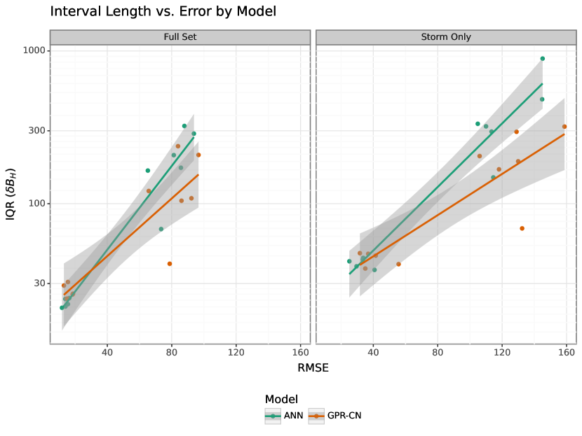
Figure 11: OLS regression on the IQR of prediction interval lengths vs. RMSE by model. Among the high RMSE stations, the IQR of prediction intervals during storms is lower for the GPR-CN model compared to the ANN. Note that the y-axis is visually log-scaled, though the units are preserved on the original scale.

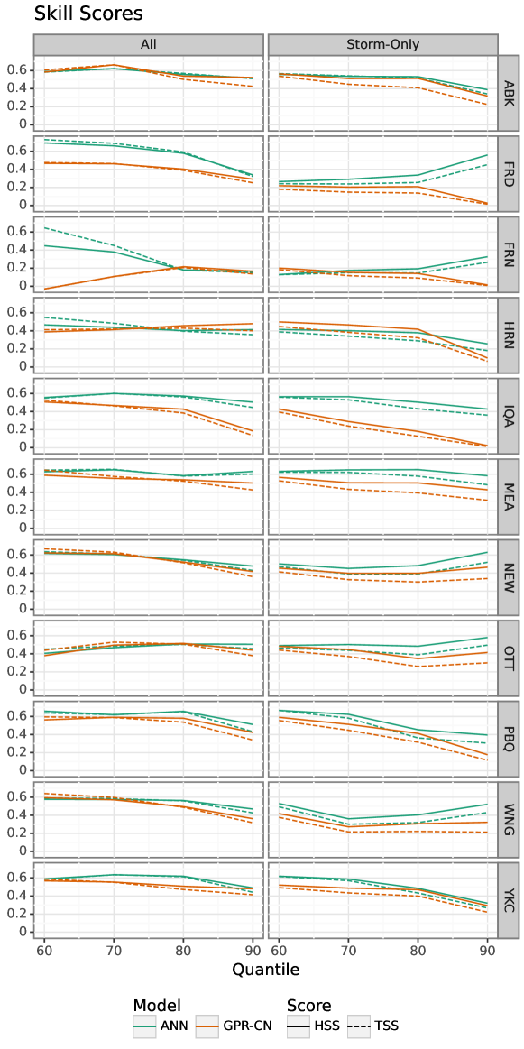
Figure 12: Skill scores for each method by station. The quantiles on the x-axis correspond to the station’s $\delta B_{H}$ quantile over the training period. These scores represent how well a model does at predicting when $\delta B_{H}$ will exceed the stated quantile. Higher is better, and the theoretical max is 1.

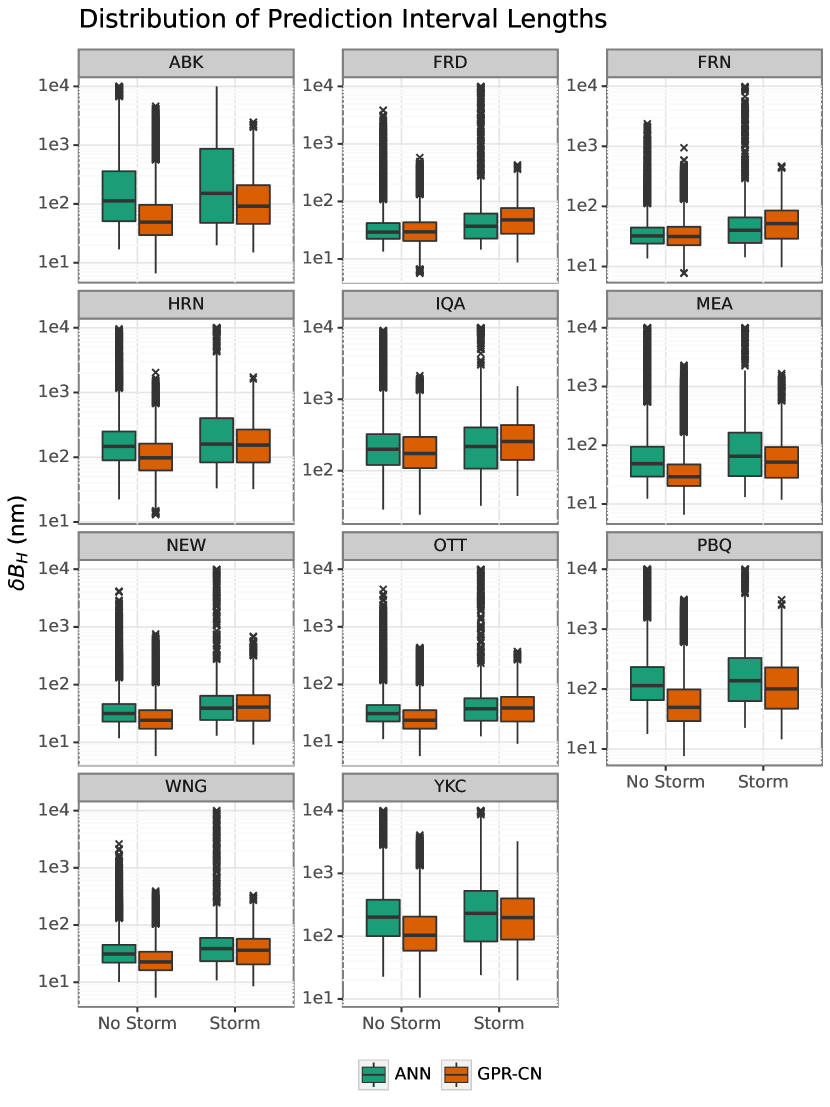
Figure 13: Distribution of interval length for storm and non-storm periods by method.

6 Conclusion

In this paper, we proposed a scalable inference algorithm for fitting sparse GPR models with contaminated normal noise. In section 4.1, we showed that the algorithm is able to correctly estimate the model hyperparameters when used to fit data simulated from the model itself. In section 4.2, we compared GPR models with different likelihoods and showed that our proposed model outperforms the others when there is a large proportion of outliers. In section 5, we applied our proposed algorithm to two real-world datasets and discussed strengths and weaknesses compared to GPR models with other robust likelihoods. In particular, our model was able to provide more informative prediction intervals for the ground magnetic perturbations dataset.

Appendix A Variational inference

Variational inference (VI) is commonly used to approximate posterior distributions in complex Bayesian models where the posterior is not tractable [38]. It provides an alternative to Markov chain Monte-Carlo (MCMC) sampling that tends to be more computationally efficient and scalable. VI approximates the posterior distribution by finding the distribution belonging to a simpler family of distributions that minimizes the Kullback-Leibler (KL) divergence with the exact posterior [38]. More concretely, suppose we have observed data, denoted by $\mathbf{y}\in\mathbb{R}^{n}$, and latent variables, denoted by $\mathbf{f}\in\mathbb{R}^{m}$. For simplicity, we assume that $\mathbf{y}$ and $\mathbf{f}$ are real-valued but that is not a requirement for VI. In the context of GPR, $\mathbf{f}$ are the latent function values. The goal of VI is to solve the following optimization problem:

$$q^{*}(\mathbf{f})=\underset{q(\mathbf{f})\in\mathcal{Q}}{\text{arg min }}\text{KL}\big{[}q(\mathbf{f})||p(\mathbf{f}|\mathbf{y})\big{]},$$ (26)

where $\mathcal{Q}$ is a family of candidate approximate distributions; and $p(\mathbf{f}|\mathbf{y})$ is the exact posterior distribution. The KL divergence between two distributions $q(\mathbf{x})$ and $p(\mathbf{x})$ is defined as

$$\text{KL}\big{[}q(\mathbf{x})||p(\mathbf{x})\big{]}=\int q(\mathbf{x})\log\frac{q(\mathbf{x})}{p(\mathbf{x})}d\mathbf{x}.$$

The resulting distribution $q^{*}(\mathbf{f})$ is then used as an approximation to the exact posterior. The difficulty of this optimization problem is dictated by the variational family $\mathcal{Q}$. Common choices include the mean-field and Gaussian variational family [39, 40]. The mean-field variational family consist of distributions that asssume the latent variables are mutually independent, i.e.

$$q(\mathbf{f})=\prod_{j=1}^{m}q_{j}(f_{m}).$$ (27)

The Gaussian variational family consists of multivariate Gaussian distributions parameterized by a mean and covariance matrix. Under this family, the optimization problem in eq. 26 simplifies to computing the mean and covariance matrix that minimizes the KL divergence. In this paper, we will focus on the Gaussian variational family. The KL divergence in eq. 26 can be decomposed as

$$\text{KL}\big{[}q(\mathbf{f})||p(\mathbf{f}|\mathbf{y})\big{]}=E_{q(\mathbf{f})}[\log q(\mathbf{f})]-E_{q(\mathbf{f})}[\log p(\mathbf{f},\mathbf{y})]+\log p(\mathbf{y}).$$ (28)

The KL divergence depends on the marginal log likelihood $\log p(\mathbf{y})$ which is almost always intractable. We can rearrange eq. 28 to express the marginal log likelihood as

$$\log p(\mathbf{y})=\text{ELBO}(q)+\text{KL}\big{[}q(\mathbf{f})||p(\mathbf{f}|\mathbf{y})\big{]}$$

where

$$\text{ELBO}(q)=E_{q(\mathbf{f})}[\log p(\mathbf{f},\mathbf{y})]-E_{q(\mathbf{f})}[\log q(\mathbf{f})].$$ (29)

This function is known as the evidence lower bound (ELBO) because it lower bounds the marginal log likelihood (or evidence). This follows from the KL divergence term being non-negative. Furthermore, since $\log p(\mathbf{y})$ is a constant with respect to $q$, maximizing the ELBO is equivalent to minimizing the KL divergence between the approximate and exact posterior, thereby solving the original optimization problem in eq. 26.

Appendix B ELBO for SVGP with Gaussian likelihood without an explicit variational distribution

We can rewrite the ELBO derived in eq. 10 as

$$\text{ELBO}=\int q(\textbf{u})\log\frac{G(\textbf{u},\textbf{y})p(\textbf{u})}{q(\textbf{u})}d\textbf{u},$$ (30)

where $\log G(\textbf{u},\textbf{y})=\int p(\textbf{f}|\textbf{u})\log p(\textbf{y}|\textbf{f})d\textbf{f}$. If we assume $p(\textbf{y}|\textbf{f})=N(\textbf{y}|\textbf{f},\sigma^{2}\textbf{I})$ (i.e. Gaussian likelihood with homoskedastic noise), then

$$\log G(\textbf{u},\textbf{y}) =\int N(\textbf{f}|\textbf{K}_{nm}\textbf{K}_{mm}^{-1}\textbf{u},\textbf{K}_{nn}-\textbf{Q}_{nn})\log[N(\textbf{y}|\textbf{f},\sigma^{2}\textbf{I})]d\textbf{f}$$

$$=\log[N(\textbf{y}|\textbf{K}_{nm}\textbf{K}_{mm}^{-1}\textbf{u},\sigma^{2}\textbf{I})]-\frac{1}{2\sigma^{2}}\text{Tr}(\tilde{\textbf{K}}_{nn}),$$

where $\tilde{\textbf{K}}_{nn}=\textbf{K}_{nn}-\textbf{Q}_{nn}$; and $\text{Tr}(\textbf{A})$ denotes the trace of matrix A. Using Jensen’s inequality, we can upper bound the ELBO in eq. 30 with

$$\text{ELBO}\leq\log\int G(\textbf{u},\textbf{y})p(\textbf{u})d\textbf{u}=\log N(\textbf{y}|0,\sigma^{2}\textbf{I}+\textbf{Q}_{nn})-\frac{1}{2\sigma^{2}}\text{Tr}(\tilde{\textbf{K}}_{nn}).$$

Therefore, under a Gaussian likelihood, the ELBO for SVGP can be maximized without explicitly assuming a variational distribuiton $q(\textbf{u})$ for the inducing points.

Appendix C ANN Fitting

Due to computational constraints, hyperparameter tuning for the ANN model is conducted on the OTT station. Hyperparameter tuning station by station for the ANN model would require moving the neural net fitting code to a GPU, a path that was not explored for this paper. Therefore, we estimate that further enhancements to the ANN model’s performance are possible. In particular, the hyperparameter optimization performed for the OTT station may not generalize well to other stations, particularly those at higher latitudes. Nonetheless, the current model serves as an adequate baseline, demonstrating comparable performance with prior works such as [34] and [36] when comparing RMSE and skill scores across all test stations.

We opt for a 4-layer deep neural network architecture. Following common convention, we incorporate the rectified linear unit (ReLU) activation function and a batch size of 32. In multivariate regression problems with time series data, it is common to face the issue of gradient explosion. To mitigate this, we utilize the AdamW optimizer with a weight decay of 0.01 and implement gradient clipping with a maximum norm of 1.0. To further reduce overfitting, early stopping is employed after 5 epochs without improvement. The optimization of additional hyperparameters is facilitated by the Bayesian Optimization library [33], by randomly selecting 20 initial combinations of hyperparameters and conducting 40 further iterations. This procedure is iterated multiple times to identify a stable set of parameters. The learning rate is adjusted using an exponential decay schedule, and dropout layers are introduced following each hidden layer at the same rate. The weight of the loss function is also tuned in this process, so we utilize RMSE as the evaluation metric on our validation set. Hyperparameter tuning results are detailed in table 6.

Layer width	Learning rate	Learning rate decay	Dropout rate	$\lambda$
100-100-80-80-2	0.00008	0.8	0.1	50

Table 6: ANN model hyperparameters tuned by Bayesian-Optimization.

It is noteworthy that our ANN models tend to produce overly broad confidence intervals, particularly for extreme events and during storm periods. To address this issue, we predict a transformed scale parameter $\tilde{\sigma}^{2}$, with the final scale parameter $\hat{\sigma}^{2}$ calculated as

$$\hat{\sigma}^{2}=\frac{C}{1+e^{-A(\tilde{\sigma}^{2}-B)}},$$

where $A$, $B$, and $C$ are tunable hyperparameters ensuring that $\hat{\sigma}^{2}$ falls within the range $[0,C]$. After exploratory adjustments, these parameters are set to $A=0.01$, $B=500$, and $C=1000$. Though this change reduces interval length in extreme cases, it does not eliminate the problem of exploding interval lengths completely.

References

- [1] Jesper W. Gjerloev. The SuperMAG data processing technique. Journal of Geophysical Research, 117, 2012.
- [2] C. J. Schrijver, R. Dobbins, W. Murtagh, and S. M. Petrinec. Assessing the impact of space weather on the electric power grid based on insurance claims for industrial electrical equipment. Space Weather, 12(7):487–498, 2014. _eprint: https://agupubs.onlinelibrary.wiley.com/doi/pdf/10.1002/2014SW001066.
- [3] Natalia E. Papitashvili and Joseph H. King. OMNI 1-min Data. NASA Space Physics Data Facility, 2020. https://doi.org/10.48322/45bb-8792, Accessed on Sept. 1, 2021.
- [4] John R. Gleason. Understanding Elongation: The Scale Contaminated Normal Family. Journal of the American Statistical Association, 88(421):327–337, 1993. Publisher: [American Statistical Association, Taylor & Francis, Ltd.].
- [5] G. E. P. Box and G. C. Tiao. A Bayesian Approach to Some Outlier Problems. Biometrika, 55(1):119–129, 1968. Publisher: [Oxford University Press, Biometrika Trust].
- [6] Anita C. Faul and Michael E. Tipping. A Variational Approach to Robust Regression. In Georg Dorffner, Horst Bischof, and Kurt Hornik, editors, Artificial Neural Networks — ICANN 2001, pages 95–102, Berlin, Heidelberg, 2001. Springer Berlin Heidelberg.
- [7] Stéphane Lathuilière, Pablo Mesejo, Xavier Alameda-Pineda, and Radu Horaud. DeepGUM: Learning Deep Robust Regression with a Gaussian-Uniform Mixture Model. In Vittorio Ferrari, Martial Hebert, Cristian Sminchisescu, and Yair Weiss, editors, Computer Vision – ECCV 2018, volume 11209, pages 205–221. Springer International Publishing, Cham, 2018. Series Title: Lecture Notes in Computer Science.
- [8] Shuang Xu and Chun-Xia Zhang. Robust sparse regression by modeling noise as a mixture of gaussians. Journal of Applied Statistics, 46(10):1738–1755, July 2019.
- [9] Anahita Sadeghian, Nabil Magbool Jan, Ouyang Wu, and Biao Huang. Robust probabilistic principal component regression with switching mixture Gaussian noise for soft sensing. Chemometrics and Intelligent Laboratory Systems, 222:104491, 2022.
- [10] M. Kuss. Gaussian Process Models for Robust Regression, Classification, and Reinforcement Learning. PhD thesis, Technische Universität Darmstadt, 2006.
- [11] Atefeh Daemi, Hariprasad Kodamana, and Biao Huang. Gaussian process modelling with Gaussian mixture likelihood. Journal of Process Control, 81:209–220, September 2019.
- [12] Andrew Naish and S. Holden. Robust Regression with Twinned Gaussian Processes. In NIPS, 2007.
- [13] Pasi Jylänki, Jarno Vanhatalo, and Aki Vehtari. Robust Gaussian Process Regression with a Student- t Likelihood. Journal of Machine Learning Research, 12, June 2011.
- [14] Zhao-Zhou Li, Lu Li, and Zhengyi Shao. Robust Gaussian Process Regression Based on Iterative Trimming. Astronomy and Computing, 36:100483, July 2021. arXiv:2011.11057 [astro-ph, stat].
- [15] Pooja Algikar and Lamine Mili. Robust Gaussian Process Regression with Huber Likelihood, January 2023. Number: arXiv:2301.07858 arXiv:2301.07858 [stat].
- [16] Haitao Liu, Yew-Soon Ong, Xiaobo Shen, and Jianfei Cai. When Gaussian Process Meets Big Data: A Review of Scalable GPs, April 2019. Number: arXiv:1807.01065 arXiv:1807.01065 [cs, stat].
- [17] Joaquin Quiñonero-Candela and Carl Edward Rasmussen. A Unifying View of Sparse Approximate Gaussian Process Regression. Journal of Machine Learning Research, 6(65):1939–1959, 2005.
- [18] Matthias W. Seeger, Christopher K. I. Williams, and Neil D. Lawrence. Fast Forward Selection to Speed Up Sparse Gaussian Process Regression. In Christopher M. Bishop and Brendan J. Frey, editors, Proceedings of the Ninth International Workshop on Artificial Intelligence and Statistics, volume R4 of Proceedings of Machine Learning Research, pages 254–261. PMLR, January 2003.
- [19] Edward Snelson and Zoubin Ghahramani. Sparse Gaussian Processes using Pseudo-inputs. In Y. Weiss, B. Schölkopf, and J. Platt, editors, Advances in Neural Information Processing Systems, volume 18. MIT Press, 2005.
- [20] Edward Snelson and Zoubin Ghahramani. Local and global sparse Gaussian process approximations. Journal of Machine Learning Research - Proceedings Track, 2:524–531, 2007.
- [21] Miguel Lázaro-Gredilla and Aníbal Figueiras-Vidal. Inter-domain Gaussian Processes for Sparse Inference using Inducing Features. In Y. Bengio, D. Schuurmans, J. Lafferty, C. Williams, and A. Culotta, editors, Advances in Neural Information Processing Systems, volume 22. Curran Associates, Inc., 2009.
- [22] Michalis Titsias. Variational Learning of Inducing Variables in Sparse Gaussian Processes. In David van Dyk and Max Welling, editors, Proceedings of the Twelth International Conference on Artificial Intelligence and Statistics, volume 5 of Proceedings of Machine Learning Research, pages 567–574, Hilton Clearwater Beach Resort, Clearwater Beach, Florida USA, April 2009. PMLR.
- [23] James Hensman, Nicolo Fusi, and Neil D. Lawrence. Gaussian Processes for Big Data. Technical Report arXiv:1309.6835, arXiv, September 2013. arXiv:1309.6835 [cs, stat] type: article.
- [24] James Hensman, Alexander Matthews, and Zoubin Ghahramani. Scalable Variational Gaussian Process Classification. In Guy Lebanon and S. V. N. Vishwanathan, editors, Proceedings of the Eighteenth International Conference on Artificial Intelligence and Statistics, volume 38 of Proceedings of Machine Learning Research, pages 351–360. PMLR, May 2015.
- [25] Jacob R. Gardner, Geoff Pleiss, David S. Bindel, Kilian Q. Weinberger, and Andrew Gordon Wilson. GPyTorch: Blackbox Matrix-Matrix Gaussian Process Inference with GPU Acceleration. In Neural Information Processing Systems, 2018.
- [26] Carl Edward Rasmussen and Christopher K. I. Williams. Gaussian Processes for Machine Learning (Adaptive Computation and Machine Learning). The MIT Press, 2005.
- [27] Andrew Gelman, Jessica Hwang, and Aki Vehtari. Understanding predictive information criteria for Bayesian models. Statistics and Computing, 24(6):997–1016, November 2014.
- [28] Qing Liu and Donald A. Pierce. A Note on Gauss-Hermite Quadrature. Biometrika, 81(3):624–629, 1994. Publisher: [Oxford University Press, Biometrika Trust].
- [29] Diederik P. Kingma and Jimmy Ba. Adam: A method for stochastic optimization, 2014.
- [30] Adam Paszke, Sam Gross, Francisco Massa, Adam Lerer, James Bradbury, Gregory Chanan, Trevor Killeen, Zeming Lin, Natalia Gimelshein, Luca Antiga, Alban Desmaison, Andreas Köpf, Edward Yang, Zach DeVito, Martin Raison, Alykhan Tejani, Sasank Chilamkurthy, Benoit Steiner, Lu Fang, Junjie Bai, and Soumith Chintala. PyTorch: An Imperative Style, High-Performance Deep Learning Library. In Proceedings of the 33rd International Conference on Neural Information Processing Systems. Curran Associates Inc., Red Hook, NY, USA, 2019.
- [31] Radford M. Neal. Monte Carlo Implementation of Gaussian Process Models for Bayesian Regression and Classification. arXiv: Data Analysis, Statistics and Probability, 1997.
- [32] Jerome H. Friedman. Multivariate Adaptive Regression Splines. The Annals of Statistics, 19(1), March 1991.
- [33] Fernando Nogueira. Bayesian Optimization: Open source constrained global optimization tool for Python, 2014–.
- [34] Amy M. Keesee, Victor Pinto, Michael Coughlan, Connor Lennox, Md Shaad Mahmud, and Hyunju K. Connor. Comparison of Deep Learning Techniques to Model Connections Between Solar Wind and Ground Magnetic Perturbations. Frontiers in Astronomy and Space Sciences, 7:550874, October 2020.
- [35] Vishal Upendran, Panagiotis Tigas, Banafsheh Ferdousi, Téo Bloch, Mark C. M. Cheung, Siddha Ganju, Asti Bhatt, Ryan M. McGranaghan, and Yarin Gal. Global Geomagnetic Perturbation Forecasting Using Deep Learning. Space Weather, 20(6), June 2022.
- [36] Victor A. Pinto, Amy M. Keesee, Michael Coughlan, Raman Mukundan, Jeremiah W. Johnson, Chigomezyo M. Ngwira, and Hyunju K. Connor. Revisiting the Ground Magnetic Field Perturbations Challenge: A Machine Learning Perspective. Frontiers in Astronomy and Space Sciences, 9:869740, May 2022.
- [37] E. Camporeale, M. D. Cash, H. J. Singer, C. C. Balch, Z. Huang, and G. Toth. A Gray-Box Model for a Probabilistic Estimate of Regional Ground Magnetic Perturbations: Enhancing the NOAA Operational Geospace Model With Machine Learning. J. Geophys. Res. Space Physics, 125(11), 2020.
- [38] David M. Blei, Alp Kucukelbir, and Jon D. McAuliffe. Variational Inference: A Review for Statisticians. Journal of the American Statistical Association, 112(518):859–877, April 2017. Publisher: Taylor & Francis.
- [39] Martin J. Wainwright and Michael I. Jordan. Graphical Models, Exponential Families, and Variational Inference. Foundations and Trends® in Machine Learning, 1(1–2):1–305, 2007.
- [40] Manfred Opper and Cédric Archambeau. The Variational Gaussian Approximation Revisited. Neural Computation, 21(3):786–792, March 2009.