Backpropagation-Based Analytical Derivatives of EKF Covariance for Active Sensing

Abstract

To enhance accuracy of robot state estimation, perception-aware (or active sensing) methods seek trajectories that minimize uncertainty. To this aim, one possibility is to seek trajectories that minimize the final covariance of an extended Kalman filter (EKF), w.r.t. its control inputs over a given horizon. However, this can be computationally demanding. In this article, we derive novel backpropagation analytical formulas for the derivatives of the final covariance of an EKF w.r.t. its inputs. We then leverage the obtained analytical gradients as an enabling technology to derive perception-aware optimal motion plans. Simulations validate the approach, showcasing improvements in both estimation accuracy and execution time. Experimental results on a real large ground vehicle also support the method.

Keywords: perception-aware, extended Kalman filter, trajectory optimization, backpropagation.

1 Introduction

In robotics, perception-aware (PA) approaches, [1, 2, 3, 4], or active sensing approaches, seek trajectories that maximize information gathered from sensors so as to perform robotic tasks safely. Notably, in the context of ground vehicles, when localization is based on ranging or bearing measurements relative to beacons, the efficiency of active sensing has been shown by [5, 6]. In [7], trajectories are generated to perform optimal online calibration between GPS and inertial measurement unit (IMU), see also [8]. In [3], for visual-inertial navigation systems, the authors have optimized the duration in which landmarks remain within the field of view. In the context of simultaneous localization and mapping (SLAM), those methods pertain to active SLAM, see [9].

One way to attack active sensing is through the use of Partially Observable Markov Decision Processes (POMDPs) [10], see [11], which offer a proper mathematical framework, but whose complexity is often prohibitory [12]. Sampling-based planners [13, 14] may be subject to the same issues. A more tractable option, that we presently adopt, is to work with the widespread extended Kalman filter (EKF), which estimates in real time the state $x_{n}$ from various sensor measurements, and (approximately) conveys the associated extent of uncertainty through the state error covariance matrix $P_{n}$, that may be used as an objective to minimize, as advocated in, e.g., [15].

Using the Gramian matrix to elicit observability, or as a surrogate for $P_{n}$, as advocated in [5, 6, 7, 16], is somewhat simpler but may lead to suboptimal motion plans in terms of gathered information [17]. Direct minimization of the final uncertainty encoded in $P_{N}$ is advocated instead in [17, 18, 15]. To find optimal trajectories, one may restrict the problem to the class of differentially flat systems, and use splines, as advocated in [18, 5], or one can try to compute and use directly the gradients of $P_{N}$ with respect to (w.r.t.) the control inputs. To this aim, several approaches are possible. One can use a brute force approach (in the vein of [19]) or numerical differentiation, that may be ill-conditioned and intractable, owing to the complexity of the EKF’s equations. To get around those problems, [15] advocates using backpropagation, through automatic differentiation, and argues that deriving analytical expressions would be difficult.

In this paper, we fill a gap by providing closed-form analytical expressions for the derivatives of any smooth function of the final covariance matrix $P_{N}$ of an EKF, w.r.t. all previous control inputs. Those novel equations, that build upon our recent results for the linear Kalman filter [20], extend them to the nonlinear case, using an EKF. In addition to being analytical, and decreasing some numerical errors, these equations lead to further speedups even over automatic differentiation, as we will show in this paper. Then, we apply the technique to derive a novel method for perception-aware optimal motion planning.

The main contributions of this paper are as follows:

• Deriving novel analytical backpropagation equations for the gradient of the covariance of an EKF with respect to all inputs of the filter, including control variables, thus partly extending [20] to the relevant nonlinear context;

• Hence providing a computationally efficient method whose cost to compute the gradients w.r.t. all control inputs at once, over an $N$-step horizon, is similar to that of running one EKF over this horizon,

• Applying the technique to derive a computationally efficient perception-aware method;

• Validate and compare the technique through simulations, and real experiments on a car-size ground vehicle.

Section 2 introduces the considered problem regarding gradient computation. Section 3 establishes backpropagation equations for computing this gradient. In Section 4, our path planning formulation is introduced. Finally, we demonstrate the benefits of our approach in simulations (Section 5) and real experiments (Section 6).

2 Gradient of the EKF’s covariance

For partially observed linear dynamical systems affected by white Gaussian noise, the Kalman filter (KF) computes the statistics of the state given past observations, namely $p(x_{n}|y_{0},\dots,y_{n})$, in real time. The Kalman filter (KF) relies on many parameters encoded in the noise covariance matrices $Q_{n}$ and $R_{n}$. There exists various approaches to compute the derivatives of the KF’s outputs w.r.t. those parameters. The early sensitivity equations [21], see also [22], allow for computing the derivative of the likelihood $\mathcal{L}:=\log p(y_{0},\dots,y_{n})$ w.r.t. the noise parameters. A much faster approach is to use backpropagation, either using numerical auto-differentiation, as advocated in [15], or closed-form formulas as very recently derived in [20].

In this paper, we target closed-form backpropagation formulas for computing the gradients of an EKF’s final covariance w.r.t. its inputs, including the control inputs. This will provide a nontrivial (partial) extension of the results of [20] to nonlinear systems. We start with a few primers.

2.1 Preliminaries

Let’s consider a nonlinear discrete-time system:

$$\left\{\begin{aligned} &x_{n}=f(x_{n-1},u_{n},w_{n}),\quad x_{0}=x^{0}\\ &y_{n}=h(x_{n})+v_{n}\end{aligned}\right.$$ (1)

where $x_{n}\in\mathbb{R}^{p}$ is the system’s state, $u_{n}\in\mathbb{R}^{q}$ is the control input, $w_{n}\in\mathbb{R}^{r}$ represents the process noise which follows a Gaussian distribution with zero mean and covariance matrix $Q_{n}$. The measured output is denoted by $y_{n}\in\mathbb{R}^{l}$, corrupted by a Gaussian measurement noise $v_{n}$ with zero mean and covariance matrix $R_{n}$. Owing to unknown noises corrupting the equations, and to the state being only partially observed through $y_{n}$, one needs to resort to a state estimator.

The Extended Kalman Filter (EKF) provides a joint estimation of the state, denoted as $\hat{x}_{n}$, and its covariance matrix, denoted as $P_{n}$, consisting of two steps.

At the propagation step, the estimated state is evolved through the noise-free model, that is,

$$\hat{x}_{n|n-1}=f(\hat{x}_{n-1|n-1},u_{n},w_{n}),$$ (2)

and the covariance of the state error is evolved as

$$P_{n|n-1} =F_{n}P_{n-1|n-1}F_{n}^{T}+G_{n}Q_{n}G_{n}^{T}\,.$$ (3)

At the update step, the estimated state and the covariance matrix are updated in the light of observation $y_{n}$ as

$$S_{n} =H_{n}P_{n|n-1}H_{n}^{T}+R_{n}\,,$$ (4)

$$K_{n} =P_{n|n-1}H_{n}^{T}S_{n}^{-1}\,,$$ (5)

$$\hat{x}_{n|n} =\hat{x}_{n|n-1}+K_{n}(y_{n}-h(\hat{x}_{n|n-1}))$$ (6)

$$P_{n|n} =(I-K_{n}H_{n})P_{n|n-1}.$$ (7)

The Riccati update step (7) proves equivalent to the following update in so-called information form:

$$P_{n|n}^{-1}=P_{n|n-1}^{-1}+H_{n}^{T}R_{n}^{-1}H_{n}.$$ (8)

In these equations, matrices $F_{n}$, $G_{n}$ and $H_{n}$ are all jacobians that depend on state estimation $\hat{x}_{n}$ and control inputs $u_{n}$:

$$F_{n} =\frac{\partial f}{\partial x_{n}}(\hat{x}_{n-1|n-1},u_{n},0)\,,\quad G_{n}=\frac{\partial f}{\partial w_{n}}(\hat{x}_{n-1|n-1},u_{n},0)\,,$$ (9)

$$H_{n} =\frac{\partial h}{\partial x_{n}}(\hat{x}_{n|n-1}).$$

Through the Jacobians, the control inputs affect the covariance matrices, which is in contrast with the linear case where all trajectories are equivalent. It thus makes sense to compute the sensitivity of covariance matrices w.r.t. control inputs.

2.2 Backpropagation based gradient computation

The final covariance computed in the EKF $P_{N|N}$ over a fixed window, say $n=0,\dots,N$, is the result of an iterative algorithm (2)-(9), and can thus be viewed as a composition of many functions from $n=0$ up to $N$, as layers in a neural network. As a result, it lends itself to backpropagation, a way of computing the chain rule backwards. Backpropagation (“backprop”) is very efficient when there are numerous inputs and the output is a scalar function (as opposed to the more intuitive method of applying the chain rule forward). In [23], in the context of linear Kalman filtering, it is used to compute the gradient of the negative logarithm of the marginal likelihood (NLL) w.r.t all observations $y_{1},\dots,y_{N}$. In [15], perception-aware trajectory generation is performed using an optimisation-based method where gradients are computed using an automatic differentiation algorithm.

2.3 Scalar loss design

For backpropagation to be numerically efficient, one needs the objective to be a scalar function. The most common choices to reflect the final uncertainty are the trace $\mathcal{L}=Tr(P_{N|N})$, used in [17, 7, 15], or the maximum eigenvalue, which has to be regularized using Schatten’s norm, see [5]. Other possibilities revolve around the Observability Gramian (OG), to elicit observability as in [5], or maximimizing the trace (which is proved in [24] to be interpretable as a deterministically propagated average error). Although the covariance matrix and the OG may be related, see [5], we will focus on the former that more realistically accounts for the noise characteristics [17].

As $Tr(P_{N|N})$ sums the diagonal terms, which are variances expressed in possibly different units and choice of scales, it is reasonable to renormalize the matrix, as suggested in [7]. Herein, we use the initial inverse covariance matrix as a scaling factor, leading to the modified trace objective $\mathcal{L}=Tr\left(P_{0}^{-1}P_{N|N}\right).$ Note that this may also ensure better conditioning of the optimization problem to come.

3 Novel sensitivity equations for the EKF

We consider a fixed window, say, $n=0\dots N$, and we seek to differentiate a function $\mathcal{L}(P_{N|N})$ of the final uncertainty $P_{N|N}$, w.r.t. all the previous EKF inputs, that are, the noise parameters $R_{n},Q_{n}$, the control inputs $u_{n}$, for $n=1\dots N$, and the initial values $\hat{x}_{0},P_{0|0}$. They all affect $\mathcal{L}(P_{N|N})$ in a complicated manner, through the EKF equations (2) to (9). For instance a modification of $u_{1}$, namely $u_{1}+\delta u_{1}$ affects initial Jacobians $R_{0},G_{0},H_{0}$ in (9), that in turn affect all subsequent quantities output by the EKF through eq. (2) to (8), finally affecting $\mathcal{L}(P_{N|N})$ in a non-obvious manner.

To analytically compute the derivatives, there are two routes. The historical one is to forward propagate a perturbation, say $\delta u_{n}$, $n\leq N$, through the equations. It is known as the sensitivity equations, and has been done–at least–for the linear Kalman filter in [21], essentially for adaptive filtering. The other route is to compute derivatives backwards, using the backprop method. It is far less straightforward, and has been proposed only very recently, leading to drastic computation speedups, see [20], in the context of linear systems. In this paper we heavily rely on our prior work [20] to go a step further, by accommodating nonlinear equations, that is, going from the Kalman Filter to the EKF, with the additional difficulty that the Jacobians depend on the estimates. Our end goal being active sensing, though, we restrict ourselves to losses of the form $\mathcal{L}(P_{N|N})$. We show this additional dependency lends itself to the backprop framework too. We also extend the calculations to get the derivatives w.r.t. the control inputs (which would not make sense in the linear case as they are null).

3.1 Matrix derivatives

We now explain the methodology, the main steps, and provide the final equations. As deriving closed-form formulas through backward computation is non trivial and lengthy, a full-blown mathematical proof can be found in the appendix.

Our method heavily relies on two ingredients. First, the notion of derivative of a scalar function w.r.t. a matrix (More detailed can be found in Appendix A), and the associated formulas based on the chain rule. Then, dependency diagrams which encapsulate how the functions are composed.

Consider $\mathcal{L}(M)$, a scalar function of a matrix defined as $M=f(X,Y)$, where $X$ and $Y$ are also matrices. $\frac{\partial\mathcal{L}}{\partial M}$ denotes the matrix defined by $(\frac{\partial\mathcal{L}}{\partial M})_{ij}=\frac{\partial\mathcal{L}}{M_{ij}}$. To alleviate notation, we similarly write $\frac{\partial\mathcal{L}}{\partial X}$ to denote the matrix $\frac{\partial\mathcal{L}\circ f}{\partial X}$.

The chain rule provides rules of calculus for matrix derivatives. We have the following formulas [25]:

$$M =XYX^{T} \Rightarrow\frac{\partial\mathcal{L}}{\partial X}=2\frac{\partial\mathcal{L}}{\partial M}XY^{T}$$ (10)

$$M =YXY^{T} \Rightarrow\frac{\partial\mathcal{L}}{\partial X}=Y^{T}\frac{\partial\mathcal{L}}{\partial M}Y$$

$$M =X^{-1} \Rightarrow\frac{\partial\mathcal{L}}{\partial X}=-M^{T}\frac{\partial\mathcal{L}}{\partial M}M^{T}$$

In the particular case where $X$ and $M$ are vectors, we have:

$$M=f(X)\Rightarrow\frac{\partial\mathcal{L}}{\partial X}=J^{T}\frac{\partial\mathcal{L}}{\partial M},$$ (11)

with $J$ the Jacobian matrix of $f$ w.r.t. $X$.

When the matrix $X$ depends on a scalar variable $s$, we have the following formula:

$$M=X(s)\Rightarrow\frac{d\mathcal{L}}{ds}=Tr\left(\frac{dX^{T}}{ds}\frac{\partial\mathcal{L}}{\partial M}\right).$$ (12)

3.2 Backprop equations for the involved matrices

The graph in Figure 1 shows the relationships involved in the calculation of the state’s error covariance, which is our variable of interest.

Figure 1: Dependencies of EKF’s variables in Riccati equations (3) and (8). Each variable (node) is a function of its predecessors.

The backprop method consists in running an EKF until time $N$, to fix the values of all variables, and then compute gradients backwards to get the derivatives. Let us assume we have computed an expression for $\frac{\partial\mathcal{L}}{\partial P_{N|N}}$ (initialization step) at final covariance $P_{N|N}$. It gives how a small variation in $P_{N|N}$ affects the objective, ignoring all the other variables. Starting with $n=N$, we go backwards as follows. As $P_{n|n}$ is a function of $P_{n|n-1}$ which is a function of $P_{n-1|n-1}$ in turn, through (3) and (8), we can use formulas (10) to assess how a small perturbation in $P_{n|n-1}$ and $P_{n-1|n-1}$ affects the loss in turn (as they affect subsequent quantities, whose variation on $\mathcal{L}$ has been computed). This yields

$$\frac{\partial\mathcal{L}}{\partial P_{n|n-1}}=(I-K_{n}H_{n})^{T}\frac{\partial\mathcal{L}}{\partial P_{n|n}}(I-K_{n}H_{n})$$ (13)

$$\frac{\partial\mathcal{L}}{\partial P_{n-1|n-1}}=F_{n}^{T}\frac{\partial\mathcal{L}}{\partial P_{n|n-1}}F_{n}$$ (14)

In the same way, we apply formula (10) to (3) and (8) to obtain the following relationships:

$$\frac{\partial\mathcal{L}}{\partial F_{n}}=2\frac{\partial\mathcal{L}}{\partial P_{n|n-1}}F_{n}P_{n-1|n-1}$$ (15)

$$\frac{\partial\mathcal{L}}{\partial G_{n}}=2\frac{\partial\mathcal{L}}{\partial P_{n|n-1}}G_{n}Q_{n}$$ (16)

$$\frac{\partial\mathcal{L}}{\partial H^{T}_{n}}=-2P_{n|n}\frac{\partial\mathcal{L}}{\partial P_{n|n}}P_{n|n}H_{n}^{T}R_{n}^{-1}$$ (17)

$$\frac{\partial\mathcal{L}}{\partial R_{n}}=R_{n}^{-1}H_{n}P_{n|n}\frac{\partial\mathcal{L}}{\partial P_{n|n}}P_{n|n}H_{n}^{T}R_{n}^{-1}$$ (18)

Knowing $\frac{\partial\mathcal{L}}{\partial P_{n|n}}$ and $\frac{\partial\mathcal{L}}{\partial P_{n|n-1}}$, these equations allow in passing to calculate the partial derivative of the loss with respect to the intermediate variables $F_{n},~{}G_{n},~{}H_{n}$ and $R_{n}$ at each step.

3.3 Backprop equations for the vector variables

We can now compute the derivatives w.r.t. the state estimates $\hat{x}$ and the control inputs $u$, which are vectors. However, a remark is necessary. Our end goal is to derive optimal controls $u_{1},\dots,u_{N}$ that minimize loss $\mathcal{L}(P_{N|N})$. As this is performed ahead of time, the (noisy) observations $y_{n}$ in (6) are not available. The most reasonable choice is then to plan using the a priori value of the $y_{n}$, i.e., $y_{n}=h(\hat{x}_{n|n-1})$. We may thus alleviate notation writing $\hat{x}_{n|n}=\hat{x}_{n|n-1}:=\hat{x}_{n}$ and $\hat{x}_{n-1|n-1}:=\hat{x}_{n-1}$.

The graph in Figure 1 only focuses on the covariance variables. If we step back, we see the Jacobians depend on the linearization point $\hat{x}_{n-1}$ and the control inputs $u_{n}$, see (9). A bigger picture encapsulating all the dependencies in the EKF is represented in Figure 2.

Figure 2: Dependency diagram of all the variables involved in an EKF.

First we compute $\frac{\partial\mathcal{L}}{\partial u_{n}}$. There is a general rule, derived from the chain rule, which is that $\frac{\partial\mathcal{L}}{\partial u_{n}}$ is the sum of all the derivatives w.r.t. the direct successors of $u_{n}$ in the graph, see e.g., [20], provided they have been already computed in a previous step of the backward calculation. Additionally using (11) and (12), and computing w.r.t. to each scalar component $u_{n}^{k}$ of vector $u_{n}$, this yields

$$\frac{\partial\mathcal{L}}{\partial u_{n}^{k}}=Tr\left(\frac{\partial\mathcal{L}}{\partial F_{n}}^{T}\frac{\partial F_{n}}{\partial u_{n}^{k}}\right)+Tr\left(\frac{\partial\mathcal{L}}{\partial G_{n}}^{T}\frac{\partial G_{n}}{\partial u_{n}^{k}}\right)+(J^{u}_{n}e_{k})^{T}\frac{\partial\mathcal{L}}{\partial\hat{x}_{n}}$$ (19)

where $J_{n}^{u}:=\frac{\partial f}{\partial u}\Bigr{|}_{\begin{subarray}{c}\hat{x}_{n-1},u_{n},0\end{subarray}}$ with $\hat{x}_{n-1},u_{n}$ computed when running the EKF forward, and $e_{k}$ the $k$-th vector of the canonical basis (details are given Appendix B).

Similarly, we compute the derivative w.r.t. the $k$-th scalar component of the system’s state $x_{n-1}^{k}$, by adding terms corresponding to each successor in the graph:

$$\frac{\partial\mathcal{L}}{\partial\hat{x}_{n-1}^{k}}=Tr\left(\frac{\partial\mathcal{L}}{\partial H_{n-1}}^{T}\frac{\partial H_{n-1}}{\partial\hat{x}_{n-1}^{k}}\right)+Tr\left(\frac{\partial\mathcal{L}}{\partial R_{n-1}}^{T}\frac{\partial R_{n-1}}{\partial\hat{x}_{n-1}^{k}}\right)$$ (20)

$$+(J^{x}_{n}e_{k})^{T}\frac{\partial\mathcal{L}}{\partial\hat{x}_{n}}+Tr\left(\frac{\partial\mathcal{L}}{\partial F_{n}}^{T}\frac{\partial F_{n}}{\partial\hat{x}_{n-1}^{k}}\right)+Tr\left(\frac{\partial\mathcal{L}}{\partial G_{n}}^{T}\frac{\partial G_{n}}{\partial\hat{x}_{n-1}^{k}}\right)$$

where $J_{n}^{x}:=\frac{\partial f}{\partial x}\Bigr{|}_{\begin{subarray}{c}\hat{x}_{n-1},u_{n},0\end{subarray}}$, which is equal to $F_{n}$.

3.4 Backprop initialization

To initialize the backward process, one needs to compute $\frac{\partial\mathcal{L}(P_{N|N})}{\partial P_{N|N}}.$ This depends on the retained loss, see Section 2.3. In the case of the normalized trace loss, we have [25]

$$\frac{\partial\mathcal{L}(P_{N|N})}{\partial P_{N|N}}=\frac{\partial Tr\left(P_{0}^{-1}P_{N|N}\right)}{\partial P_{N|N}}=P_{0}^{-1}.$$ (21)

In the case where one targets the maximum eigenvalue of $P_{N|N}$ as a minimization objective, the loss must be chosen consequently. To handle the non differentiability of this cost function, we resort to its regularized version using Schatten’s norm, see [5].

Note also that at $n=N$, (20) needs to be adapted, as $\hat{x}_{N}$ only has two successors in the graph, thus:

$$\frac{\partial\mathcal{L}}{\partial\hat{x}_{N}^{k}}=Tr\left(\frac{\partial\mathcal{L}}{\partial H_{N}}^{T}\frac{\partial H_{N}}{\partial\hat{x}_{N}^{j}}\right)+Tr\left(\frac{\partial\mathcal{L}}{\partial R_{N}}^{T}\frac{\partial R_{N}}{\partial\hat{x}_{N}^{k}}\right)$$ (22)

3.5 Final equations

The gradients may be obtained as follows. We first run the EKF forward, to get all the EKF variables given a sequence of inputs. Then, we may compute the derivative of the loss w.r.t. $P_{N|N}$ at the obtained final covariance matrix. Letting $n=N,$ (17)-(18), provide the derivatives w.r.t. $H_{N}$ and $R_{N}$, and (13) w.r.t. $P_{N|N-1}$. In turn (22) provides the derivative w.r.t. $\hat{x}_{N}$, so that (19) yields the gradient w.r.t. control input $u_{N}$. Continuing the process backward and using the equations above, we get the derivatives w.r.t. to all control inputs. A summary of the equations is given in Appendix D.

The process allows for drastic computation speedups, as the backward equations yield derivatives w.r.t. all control inputs in one pass only. By contrast, forward propagating perturbations would demand running an entire EKF-like process from scratch for $k=n$ to $N$ to derive the derivative w.r.t. $u_{n}$. Akin to dynamic programming, backpropagation allows for reusing previous computations at each step.

4 Application to perception-aware planning

The computation of the gradients w.r.t. all the EKF’s variables is a contribution in itself that may prove useful beyond active sensing. However, our present goal is to leverage it to address the following perception-aware optimal path planning problem:

$$\left\{\begin{aligned} &\underset{x_{1},\dots,x_{N},u_{1},\dots,u_{N}}{\min}\mathcal{L}(P_{N|N})\\ \text{s.t.}~{}&\\ &\forall n\leq N~{}x_{n}=f(x_{n-1},u_{n},w_{n}),\quad x_{0}=x_{I},\\ &\forall n\leq N~{}P_{n|n-1}=F_{n}P_{n-1|n-1}F_{n}^{T}+G_{n}Q_{n}G_{n}^{T},\\ &\forall n\leq N~{}P_{n|n}=(I-K_{n}H_{n})P_{n|n-1},\\ &\forall n\leq N~{}u_{\min}\leq u_{n}\leq u_{\max}\end{aligned}\right.$$ (23)

where $N$ is the time horizon, and $\mathcal{L}$ a scalar loss. This approach is known as partial collocation, as in [15], i.e., we explicitly include states as optimization variables and implicitly compute the covariance. A commonly employed method for solving this problem involves a first-order optimization algorithm, the main steps of which are outlined in Algorithm 1. From a computational perspective, the gradient computation stands out as the most computationally demanding step, hence the interest for the method developed above.

While (23) seeks trajectories that minimize the accumulated uncertainty on the robot state over a given horizon, we note that it is easy to add constraints or another term in the loss to perform a specific task. For example, adding the constraint $x_{N}=x_{F}$ allows for reaching a specific state while being perception-aware. Note it is also easy to make $\mathcal{L}$ depend on previous $P_{n|n}$, $n<N$, as in [7].

4.1 Algorithm

With known gradients, a first order nonlinear optimization algorithm such as Sequential Quadratic Programming (SQP) may be brought to bear. This leads to Algorithm 1.

Algorithm 1 Path planning algorithm

$x_{0},~{}P_{0},~{}N,\mathcal{L}$

$u\leftarrow(u_{0},\dots,u_{N})$

while $\mathcal{L}(P_{N|N})$ not converge do

     $g\leftarrow$ gradient_computation$(u)$

     $\alpha\leftarrow$ line_search$(u,g)$

     $u\leftarrow$ update$(u,g,\alpha)$ $\triangleright$ Using SQP for example

end while

Return: $(u_{0},\dots,u_{N})$

The process involves computing the gradient $g$ of the cost function w.r.t. the control variables using forward and backward passes through the EKF. Additionally, we compute the gradient of the constraints with respect to decision variables. Subsequently, line search is conducted to determine an appropriate step size $\alpha$ for efficient convergence. However, line search requires evaluating the cost function, which corresponds to running a full EKF in our case. The decision variables are then updated using SQP. Further details are given in the experimental sections.

4.2 Discussion

In prior work, it proved difficult to use a loss $\mathcal{L}$ depending on the state’s covariance $P_{N|N}$. Indeed, the gradient computation of the loss w.r.t each control variable is expensive when using forward difference [7, 17], as explained in Section 3.5. This has motivated [15] to use backpropagation, through automatic differentiation (AD). [15] also argues deriving analytical formulas would be difficult.

The interest of our work, that provides analytical formulas, is twofold in this regard. First, it is often preferable to have closed-form formulas when possible, to rule out many numerical errors and keep better control over the calculation process (possibly opening up for some guarantees about the execution). As efficient implementations of the EKF involve Cholesky or SVDs of the covariance matrix, the behaviour of AD seems difficult to anticipate or guarantee. Then, it leads to computation speedups, as it will be shown experimentally in the sequel.

5 Simulation results

We now apply our results to the problem of wheeled robot localization. We consider a car-like robot modelled through the unicycle equations, and equipped with a GPS returning position measurements. There are two difficulties associated with this estimation problem. First, the heading is not directly measured. Then, and more importantly, we assume that the position of the GPS antenna in the robot’s frame (we call lever arm) is unknown, or inaccurately known, or may slightly vary over time. The resulting problem pertains to simultaneous self-calibration and navigation, in the vein of [7] but in a simpler context. In straight lines, for instance, the lever arm is not observable, so perception-aware trajectories should lead to more accurate robot state estimation.

In this section we present the model, and we assess and compare our method through simulations. In the next section, we apply it to a real world off-road vehicle.

5.1 Robot model

The system state consists of the orientation (heading) $\theta_{n}\in\mathbb{R}$ in 2D, the position of the vehicle $p_{n}\in\mathbb{R}^{2}$, and the lever arm $l_{n}\in\mathbb{R}^{2}$. The control inputs are the steering angle $\nu_{n}$ and the forward velocity $\mu_{n}$. The kinematic equations based on a roll-without-slip assumption are as follows:

$$\left\{\begin{aligned} &\theta_{n}=\theta_{n-1}+\frac{dt}{L}(\mu_{n}+w_{n}^{\mu})\tan(\nu_{n}+w_{n}^{\nu}),\\ &p_{n}=p_{n-1}+dt\Omega\left(\theta_{n-1}\right)(\mu_{n}+w_{n}^{\mu})e_{1},\\ &l_{n}=l_{n-1}\end{aligned}\right.$$ (24)

where $\Omega(\theta)=\begin{pmatrix}\cos(\theta)&-\sin(\theta)\\ \sin(\theta)&\cos(\theta)\end{pmatrix}$, $L$ is the distance between the front and the rear wheels, $e_{1}=(1,0)^{T}$ indicates that the velocity is aligned with the robot’s heading, and $dt$ is the sampling time. A Gaussian white noise $w_{n}=(w_{n}^{\mu},w_{n}^{\nu})^{T}$ with covariance matrix $Q$ corrupts the forward velocity $\mu_{n}$ and steering angle $\nu_{n}$ to account for actuators’ imperfections, and the mismatch with idealized kinematic model, i.e., slip.

Letting $l_{n}\in\mathbb{R}^{2}$ be the position of the GPS antenna in the vehicle’s frame w.r.t. to its center (the midpoint of the rear axle), the position measured by the GPS is

$$y_{n}=p_{n}+\Omega(\theta_{n})l_{n}+\epsilon_{n}$$ (25)

where $\epsilon_{n}$ is a 2D white noise with covariance matrix $R_{n}$.

In the simulations, we let $L=4$m, $dt=1s$. In terms of noise parameters, we let $Q=\mathrm{diag}(0.1,\pi/180)$, and $R_{n}$ be the identity matrix, i.e., a standard deviation of 1 m for the GPS position measurements. To account for actuator physical limits, we assume $|\nu_{n}|\leq 30\pi/180$ rad and $0\leq\mu_{n}\leq 5$ m.s^-1. To account for acceleration limits, we add the constraints $|\Delta\nu_{n}|\leq 15\pi/180$ rad.s^-1 and $|\Delta\mu_{n}|\leq 1$ m.s^-2.

5.2 Simulation results

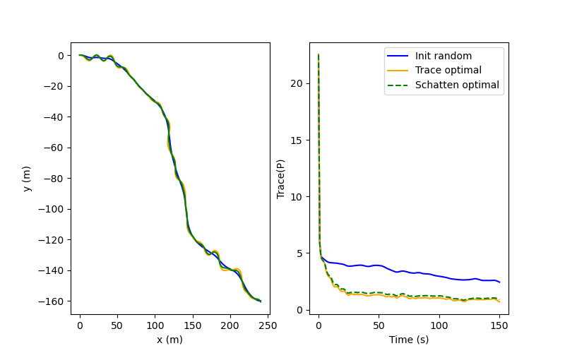
Figure 3: On the left, an example of an initial random guess in blue. The other two trajectories are solutions to the perception-aware problem where the loss is the trace (in orange) and the Schatten norm (in green). The right plot shows the expected trace of the covariance evolution for each trajectory.

We start by sampling admissible control inputs over a horizon $N=150$s. Then, the corresponding trajectory is obtained by integration. We then use the sequential least-squares programming (SLSQP) algorithm from Scipy [26] to optimize the sequence of controls to apply. The calculation of the gradient of the loss with respect to the control inputs is performed using the equations detailed in Section 3. An example of the initial random trajectory and the solution of the perception-aware problem can be found in Figure 3. The optimal trajectory for the Schatten norm and for the trace are quite similar in this case, and both oscillate around the initial random trajectory. These oscillations are manoeuvres that increase the observability of the lever arm. They lead to an actual reduction of the expected theoretical error covariance.

To demonstrate that the final covariance minimization translates into an actual reduction of the average state estimation error, we simulate 200 trials of each optimal trajectory by adding process noise and observation noise. During the simulation, the state is estimated with an EKF based on (24), (25). The evolution of the absolute estimation error of the lever arm is displayed on Figure 4. For PA trajectories, the error decreases and converges more rapidly, illustrating the benefit of perception-aware optimal trajectory generation.

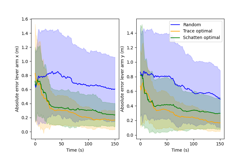
Figure 4: Absolute estimation error of the lever arm during the trajectory. On the left the error for the lever arm in x and on the right in y. One-$\sigma$ envelope illustrates the dispersion of errors over trials.

5.3 Computation time

We compared the computation times for the gradient of the loss w.r.t. control inputs with three different methods. The first method uses (forward) finite differences to compute the gradient, as in [27]. The second method is an automatic differentiation method, which adopts the backpropagation paradigm, but through a numerical tool, akin to [15]. Namely, we used the state-of-the-art PyTorch automatic differentiation (AD) [28]. Finally, the last method uses our backpropagation analytical formulas of Section 3. The code was executed on computer with an Intel Core i5 at 2.60 GHz.

Table 1: Average and standard deviation of gradient calculation time (over 100 calculations) using different methods.

Method	Execution time
Finite differences	26.92 $\pm$ 8.45s
PyTorch Autograd	0.55 $\pm$ 0.19s
Ours	0.19 $\pm$ 0.07s

Table 1 shows that gradient calculation using backpropagation (Autograd and ours) leads to large speedups. Indeed, when using a finite difference based method, optimization is computationally expensive, as mentioned in [7], where optimizing the trace of the sum of all covariances is reported to take 13 hours for a 3D inertial navigation system. Even when compared to state-of-the-art PyTorch Autograd, our closed-form formulas are much faster, and more stable in terms of variability of computation time.

The computation time for the complete resolution of the optimization problem (23) using our gradient calculation method and Algorithm 1 is 351s. Although this perfectly suits off-line trajectory generation, it means the robot should stop for a few minutes to plan in a real-time context.

5.4 Discussion

A few remarks are in order. First, we see that, by replacing state-of-the-art autograd differentiation with our formulas, one may (roughly speaking) double the planning horizon for an identical computation budget. Besides, analytical formulas better suit onboard implementation. It is interesting to note that they are totally akin to the EKF equations, which must be implemented on the robot anyway. Finally, analytical formulas–when available–may be preferable to numerical methods, as one keeps a better control over what is being implemented, possibly opening up for some guarantees (the behavior of autograd may be harder to anticipate, and leads to higher computation time variability). Moreover, we anticipate that coding them in C++ may lead to further speedups.

Note that the overall computation time of the path planning algorithm could be significantly reduced. First, we may obviously optimize over a shorter horizon. Then, the optimizer currently uses a line search algorithm to determine the descent step size. In our case, evaluating the objective function is computationally expensive because it requires running the EKF. Therefore, finding a method that reduces the number of calls to the objective function should prove efficient. Finally, another option to reduce computation time is to decrease the number of decision variables, by for instance parameterizing trajectories using B-splines, as in [5].

We may also comment on the obtained trajectories. As the optimization problem is highly nonlinear, non-convex, and constrained, one should expect an optimization method to fall into a close-by local minimum. In Figure 3, the local nature of the optimum proves visible, as the obtained trajectory oscillates around the initial trajectory. Methods to step out of local minima go beyond the scope of this paper. However, it is worth noting that albeit a (close-by) local minimum, the obtained trajectory succeeds in much reducing state uncertainty. It reduces the final average error on the lever arm, which is the most difficult variable to estimate, by a factor 3, see Figure 4.

In the context of real-time online planning, this suggests a sensible way to use the formulas of the present paper would be to compute a real-time trajectory that optimizes a control objective, and then to refine it in real time, by performing a few gradient descent steps. This shall (much) increase the information gathered by the sensors.

6 Real-world experiments

Real experiments were conducted jointly with the company Safran, a large group that commercializes (among others) navigation systems. With the help from its engineers, we used an experimental off-road car owned by the company, which is approximately 4m long and 2.1m wide.

6.1 Experimental setting

The vehicle is equipped with a standard GPS, odometers, and a RTK (Real Time Kinematic) GPS, which is not used by the EKF, but serves as ground-truth for position owing to its high accuracy. The lever arm between the GPS and the RTK is denoted by $l_{GPS/RTK}$, and has been calibrated (it is only used for comparison to the ground-truth).

To further test our method, we conducted localization experiments on both ordinary and PA trajectories and compared their performance. We used the model described in Section 5.1, and devised an EKF that fuses odometer data (dynamical model) with GPS position measurements. The vehicle state is represented by a 5-dimensional vector: two dimensions for position, one for the orientation, and two for the lever arm between the GPS and the center of the vehicle frame (midpoint of the rear axle).

Initially, we generated ordinary trajectories at two different speeds (5 $km/h$, 10 $km/h$). Subsequently, we employed our PA path planning Algorithm 1 initialized with those trajectories, to address optimization problem (23), using the final covariance trace as the loss. The constraints used were those relative to the actuators. To demonstrate the ability of optimization-based planning methods to handle further constraints, we also constrained the distance between the initial trajectory and the PA trajectory to be less than 1.5m. Then, we used local tangent plane coordinates computed near the experiment locations to convert 2D planning to world frame coordinates. Then, we followed each trajectory and computed the localization error committed by the EKF.

To measure localization accuracy, we utilized the RTK-GPS system as a ground-truth, since its uncertainties are of the order of a few centimeters. The position error of the vehicle was computed as follows:

$$e_{n}=\left\lVert p_{n}^{RTK}-\big{(}\hat{p}_{n}+\Omega(\hat{\theta}_{n})(\hat{l}_{n}+l_{GPS/RTK})\big{)}\right\rVert$$ (26)

6.2 Results

The off-road experiment was performed in a field. It consists of 4 runs: 2 reference runs and 2 perception-aware runs (at 5 $km/h$ and 10 $km/h$). Trajectories returned by RTK-GPS over the first run are displayed in Figure 5. We note the oscillations of the PA trajectory around the reference trajectory, enhancing state observability.

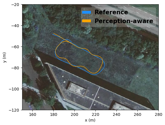
Figure 5: Off-road trajectories of the RTK-GPS in a local tangent plane coordinates oriented East-North-Up of the scenario at 5 km/h.

Figure 6 shows the trajectories for the second run, along with the evolution of the trace of $P_{n|n}$ output by the EKF (on the first run, the latter is wholly similar and was not included owing to space limitations, to improve legibility of Fig. 5). We see the improvement in terms of trace through the optimized trajectories. The visible wiggling of the covariance corresponds to the correction steps of the EKF. Indeed, the dynamical model is run at 100Hz, corresponding to the odometer frequency, while corrections are made when GPS data are available, at approximately 1Hz.

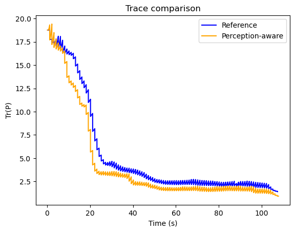
Figure 6: On the left, trajectories of the RTK-GPS in local tangent plane coordinates at 10 km/h. On the right, the evolution of the covariance trace along each trajectory in the scenario at a speed of 10 km/h.

6.3 Analysis

Although the trace of the covariance is smaller along the PA trajectory, it doesn’t necessarily guarantee that the error with respect to ground truth is reduced. The uncertainty calculated by the filter assumes all random variables are Gaussian, and the EKF is based on approximations. For each trial, we calculated the average error obtained for each type of trajectory. The results presented in Table 2 point out that PA trajectories enhance localization accuracy. Indeed, in the scenario at 5 km/h, the error decreases by $13.24\%$ between the reference and the PA trajectory, and by $8.25\%$ in the scenario at 10 km/h. However, when compared with results from simulations, the improvement is smaller. Several factors could explain this difference. Firstly, in simulations, we calculated an average result using the Monte Carlo method, whereas here we have a single trial. Additionally, in simulations, model and noises are perfectly known, whereas in reality, they are not. The roll-without-slip assumption is especially challenged when using an off-road vehicle. This also makes the trajectory tracking far from perfect. Finally, due to the limited area, we explicitly constrained the optimized trajectory to stay within a 1.5 $m$ radius around the reference one, producing a trajectory that optimally “refines” the reference trajectory, limiting the accuracy increase.

Table 2: Estimation error according to (26) for all trajectories

Speed (km/h)	Type	Mean error (m)
5	Ref	3.32
	PA	2.88
10	Ref	4.73
	PA	4.34

7 Conclusion

Our first contribution has been to introduce novel backpropagation analytical equations to compute the gradient of any loss based on the covariance of an EKF, w.r.t all its inputs. Beyond the theoretical contribution, they lead to actual numerical speedups. Our second contribution has been to leverage those formulas to address PA path planning, and to test the method in simulation and on real-world experiments over large off-road trajectories over a span of more than 50 meters. In future work, we would like to apply the method to more challenging problems, such as inertial navigation [7], and to improve its scalability, notably by improving the line search. We also would like to combine the method with other objectives such as reaching a desired goal, collision avoidance, or energy consumption.

Appendix A Matrix derivatives

First, we provide an example of how to derive matrix derivative equations. Then, we will list all the matrix derivative equations we have used in the paper. We consider a scalar function $\mathcal{L}:\mathbb{R}^{n\times n}\rightarrow\mathbb{R}$ and we define $\frac{\partial\mathcal{L}(X)}{\partial X}$ as the matrix of the derivative of $\mathcal{L}$ w.r.t each component of X (i.e. $\left(\frac{\partial\mathcal{L}(X)}{\partial X}\right)_{i,j}=\frac{\partial\mathcal{L}(X)}{\partial x_{i,j}}$). Using only matrix multiplication, we can express first-order Taylor expansion in the following form (which can alternatively be considered as a definition of the gradient):

$$\mathcal{L}(X+\delta X)=\mathcal{L}(X)+Tr\left(\left(\frac{\partial\mathcal{L}}{\partial X}\right)^{T}\delta X\right)+o\left(\delta X\right)$$ (27)

Now, let’s compute $\frac{\partial\mathcal{L}\circ\varphi(X)}{\partial X}$ when $\varphi(X)=XYX^{T}=M$ expressed as a function of $\frac{\partial\mathcal{L}}{\partial M}$.

$$\mathcal{L}\circ\varphi(X+\delta X) =\mathcal{L}((X+\delta X)Y(X+\delta X)^{T})$$ (28)

$$=\mathcal{L}(XYX^{T}+XY\delta X^{T}+\delta XYX^{T}+\delta XY\delta X^{T})$$

$$=\mathcal{L}(M)+Tr\left(\left(\frac{\partial\mathcal{L}}{\partial M}\right)^{T}(XY\delta X^{T}+\delta XYX^{T})\right)+o(\delta X)$$

$$=\mathcal{L}(M)+2Tr\left(YX^{T}\left(\frac{\partial\mathcal{L}}{\partial M}\right)^{T}\delta X\right)+o(\delta X)$$

$$=\mathcal{L}(M)+Tr\left(\left(2\frac{\partial\mathcal{L}}{\partial M}XY^{T}\right)^{T}\delta X\right)+o(\delta X)$$

On the other hand, we express the Taylor expansion of $\mathcal{L}\circ\varphi$:

$$\mathcal{L}\circ\varphi(X+\delta X) =\mathcal{L}\circ\varphi(X)+Tr\left(\left(\frac{\partial\mathcal{L}\circ\varphi}{\partial X}\right)^{T}\delta X\right)+o(\delta X)$$ (29)

$$=\mathcal{L}(M)+Tr\left(\left(\frac{\partial\mathcal{L}\circ\varphi}{\partial X}\right)^{T}\delta X\right)+o(\delta X)$$

By identification we conclude that:

$$\boxed{\frac{\partial\mathcal{L}\circ\varphi}{\partial X}=2\frac{\partial\mathcal{L}}{\partial M}XY^{T}}$$

which we write more economically as $\frac{\partial\mathcal{L}}{\partial X}=2\frac{\partial\mathcal{L}}{\partial M}XY^{T}$, since writing explicitly all the functions composed in an EKF would be impossible or extremely cluttered. Following the same proof structure, we derive:

$$M =XYX^{T} \Rightarrow\frac{\partial\mathcal{L}}{\partial X}=2\frac{\partial\mathcal{L}}{\partial M}XY^{T}$$ (30)

$$M =YXY^{T} \Rightarrow\frac{\partial\mathcal{L}}{\partial X}=Y^{T}\frac{\partial\mathcal{L}}{\partial M}Y$$

$$M =X^{-1} \Rightarrow\frac{\partial\mathcal{L}}{\partial X}=-M^{T}\frac{\partial\mathcal{L}}{\partial M}M^{T}$$

Let $A:\mathbb{R}^{q}\rightarrow\mathbb{M}^{n\times n}$, and we want to compute $\frac{\partial\mathcal{L}(A(x))}{\partial x^{j}}$ ($x^{j}$ is the $j$-th component of vector $x$) as a function of $\frac{\partial\mathcal{L}(A)}{\partial A}$. Employing the Chain rule, we have:

$$\frac{\partial\mathcal{L}\circ A}{\partial x^{j}}=Tr\left(\frac{\partial A}{\partial x^{j}}^{T}\frac{\partial\mathcal{L}}{\partial A}\right)=\sum_{k,l}\left(\frac{\partial A}{\partial x^{j}}\right)_{k,l}\left(\frac{\partial\mathcal{L}}{\partial A}\right)_{k,l}$$ (31)

Computationally, we favour the first expression.

Now, consider a scalar function $\mathcal{L}:\mathbb{R}^{n}\rightarrow\mathbb{R}$ and vector-valued function $f:\mathbb{R}^{n}\rightarrow\mathbb{R}^{n}$ with jacobian $J_{x}$. We want to compute $\frac{\partial\mathcal{L}\circ f(x)}{\partial x}$ as a function of $\frac{\partial\mathcal{L}(m)}{\partial m}$ with $m=f(x)$. Note that $\frac{\partial\mathcal{L}\circ f(x)}{\partial x}$ corresponds then to the usual (column) vector gradient $\nabla_{x}(\mathcal{L}\circ f)$. First, we write the first-order Taylor expansion of $\mathcal{L}\circ f$:

$$\mathcal{L}\circ f(x+\delta x)=\mathcal{L}\circ f(x)+\langle\nabla\mathcal{L}\circ f,\delta x\rangle+o\left(\delta x\right)$$ (32)

$$\mathcal{L}\circ f(x+\delta x) =\mathcal{L}(f(x)+J_{x}\delta x+o(\delta x))$$ (33)

$$=\mathcal{L}(f(x))+\langle\nabla\mathcal{L},J_{x}\delta x\rangle+o(\delta x)$$

$$=\mathcal{L}\circ f(x)+\langle J_{x}^{T}\nabla\mathcal{L},\delta x\rangle+o(\delta x)$$

By identification we conclude that:

$$\nabla_{x}(\mathcal{L}\circ f)=J_{x}^{T}\nabla_{m}\mathcal{L}\Leftrightarrow\frac{\partial\mathcal{L}\circ f(x)}{\partial x}=J_{x}^{T}\frac{\partial\mathcal{L}(m)}{\partial m}$$ (34)

Appendix B Backpropagation equations in an EKF

To compute the gradient w.r.t any variable using backpropagation, it is necessary to sum all contributions over the direct successors of this variable, see, e.g., [23]. The contribution of a direct successor is indicated by an exponent in brackets. Thus, for the direct successors of x denoted by $w_{i}$, the sum over all contributions is computed as follows:

$$\frac{\partial\mathcal{L}}{\partial x}=\sum_{w_{i}\text{ direct successor of }x}\left(\frac{\partial\mathcal{L}}{\partial x}\right)^{(w_{i})}$$ (35)

For the sake of simplicity, we begin by deriving equations w.r.t. the matrices involved in the Riccati equation. Subsequently, we calculate the contributions w.r.t input control variables and state vector variables.

B.1 Gradient backpropagation in Riccati equations

First we consider the propagation step:

$$\mathnormal{P}_{n|n-1} =\mathnormal{F}_{n}\mathnormal{P}_{n-1|n-1}\mathnormal{F}_{n}^{T}+G_{n}\mathnormal{Q}_{n}Gn^{T}\,,$$ (36)

followed by an update step (Riccati equation):

$$\mathnormal{S}_{n} =\mathnormal{H}_{n}\mathnormal{P}_{n|n-1}\mathnormal{H}_{n}^{T}+\mathnormal{R}_{n}\,,$$ (37)

$$\mathnormal{K}_{n} =\mathnormal{P}_{n|n-1}\mathnormal{H}_{n}^{T}\mathnormal{S}_{n}^{-1}\,,$$ (38)

$$\mathnormal{P}_{n|n} =(\mathnormal{I}-\mathnormal{K}_{n}\mathnormal{H}_{n})\mathnormal{P}_{n|n-1}\ ,$$ (39)

$$\Leftrightarrow\quad\mathnormal{P}_{n|n}^{-1} =\mathnormal{P}_{n|n-1}^{-1}+H_{n}^{T}R_{n}^{-1}H_{n}$$ (40)

We start with a graph showing the relationship between variables to get a better understanding of the dependencies between them.

Figure 7: Dependencies of KF’s variables in Riccati’s equations

For the posterior covariance, we apply equation (30) to the Ricatti equation.

$$\frac{\partial\mathcal{L}}{\partial P_{n-1|n-1}} =\left(\frac{\partial\mathcal{L}}{\partial P_{n-1|n-1}}\right)^{(P_{n|n-1})}$$ (41)

$$=\mathnormal{F}_{n}^{T}\frac{\partial\mathcal{L}}{\partial\mathnormal{P}_{n|n-1}}\mathnormal{F}_{n}$$

For the posterior covariance, we depart from the information form of the Riccati equation (40) and we find:

$$\frac{\partial\mathcal{L}}{\partial\mathnormal{P}_{n|n-1}} =-\mathnormal{P}_{n|n-1}^{-1}\left(\frac{\partial\mathcal{L}}{\partial\mathnormal{P}_{n|n-1}^{-1}}\right)^{(\mathnormal{P}_{n|n})}\mathnormal{P}_{n|n-1}^{-1}$$ (42)

$$=\mathnormal{P}_{n|n-1}^{-1}\mathnormal{P}_{n|n}\frac{\partial\mathcal{L}}{\partial\mathnormal{P}_{n|n}}\mathnormal{P}_{n|n}\mathnormal{P}_{n|n-1}^{-1}$$

$$=(\mathnormal{I}-\mathnormal{K}_{n}\mathnormal{H}_{n})^{T}\frac{\partial\mathcal{L}}{\partial\mathnormal{P}_{n|n}}(\mathnormal{I}-\mathnormal{K}_{n}\mathnormal{H}_{n}),$$

where in the last line we have used (39). Then we have:

$$\frac{\partial\mathcal{L}}{\partial\mathnormal{F}_{n}} =\left(\frac{\partial\mathcal{L}}{\partial\mathnormal{F}_{n}}\right)^{(\mathnormal{P}_{n|n-1})}=2\frac{\partial\mathcal{L}}{\partial\mathnormal{P}_{n|n-1}}\mathnormal{F}_{n}\mathnormal{P}_{n-1|n-1}$$ (43)

$$\frac{\partial\mathcal{L}}{\partial G_{n}} =\left(\frac{\partial\mathcal{L}}{\partial G_{n}}\right)^{(\mathnormal{P}_{n|n-1})}=2\frac{\partial\mathcal{L}}{\partial\mathnormal{P}_{n|n-1}}G_{n}Q_{n}$$ (44)

$$\left(\frac{\partial\mathcal{L}}{\partial H_{n}}\right)^{T} =\left(\frac{\partial\mathcal{L}}{\partial H_{n}}\right)^{(\mathnormal{P}_{n|n})}=2\frac{\partial\mathcal{L}}{\partial P_{n|n}^{-1}}H_{n}^{T}R_{n}^{-1}$$ (45)

$$=-2P_{n|n}\frac{\partial\mathcal{L}}{\partial P_{n|n}}P_{n|n}H_{n}^{T}R_{n}^{-1}$$

$$\frac{\partial\mathcal{L}}{\partial R_{n}} =\left(\frac{\partial\mathcal{L}}{\partial R_{n}}\right)^{(\mathnormal{P}_{n|n})}=-R_{n}^{-1}\frac{\partial\mathcal{L}}{\partial R_{n}^{-1}}R_{n}^{-1}$$ (46)

$$=-R_{n}^{-1}H_{n}\frac{\partial\mathcal{L}}{\partial P_{n|n}^{-1}}H_{n}^{T}R_{n}^{-1}=R_{n}^{-1}H_{n}P_{n|n}\frac{\partial\mathcal{L}}{\partial P_{n|n}}P_{n|n}H_{n}^{T}R_{n}^{-1}$$

B.2 Gradient backpropagation with respect to the controls

Assume we have a nonlinear dynamical model:

$$x_{n} =f(x_{n-1},\mathnormal{u}_{n},w_{n}),$$ (47)

$$y_{n} =h(x_{n})+\nu_{n}.$$ (48)

As before we can represent dependencies between variables using a graph:

Figure 8: Graph of dependencies of EKF’s variables involved propagation and linearization step

Returning to the Riccati equation, we are interested in using $\mathcal{L}(P_{N})$ as a cost function and we would like to assess the sensitivity of $\mathcal{L}$ w.r.t. the controls $u_{n}$’s. The influence of the controls on $\mathcal{L}$ is mediated through the parameters $F_{n}$, $G_{n}$ $H_{n}$ and $R_{n}$. Particularly, with non-linear dynamic, the elements of matrices $F_{n}$ and $G_{n}$ may exhibit dependence on both $x_{n-1}$ and $u_{n}$. Furthermore, $H_{n}$ and $R_{n}$ depend on $x_{n}$. Additionally, it is assumed that the remaining parameters in the Riccati equation remain independent of $x_{n}$ and $u_{n}$.

Note that, it proves easier to ignore the relation between function $f$ and matrices $\mathnormal{F}_{n}$. We just see the $\mathnormal{F}_{n}$’s as arbitrary functions of the variables $x_{n-1},u_{n-1}$ for now, allowing for a generic use of the notation of Jacobians that may avoid confusion.

By backpropagating the equations of the above subsection over the horizon, we have computed the sensitivity of $\mathcal{L}$ w.r.t. the various matrices at play. We now view $\mathcal{L}$ as a function of these matrices:

$$\mathcal{L}(F_{1},\dots,F_{N},G_{1},\dots,G_{N},H_{1},\dots,H_{N},R_{1},\dots,R_{N})$$

with previously computed (known) gradients $\frac{\partial\mathcal{L}}{\partial\mathnormal{F}_{n}}$, $\frac{\partial\mathcal{L}}{\partial G_{n}}$, $\frac{\partial\mathcal{L}}{\partial R_{n}}$ and $\frac{\partial\mathcal{L}}{\partial\mathnormal{H}_{n}}$. Let us replace the dynamical model above with a linearized model:

$$\left\{\begin{aligned} &x_{n}=f(x_{n-1},u_{n},w_{n})\\ &\tilde{x}_{n}=f(\tilde{x}_{n-1},u_{n},0)\end{aligned}\right.$$ (49)

$$\Rightarrow e_{n} =x_{n}-\tilde{x}_{n}=f(x_{n-1},u_{n},w_{n})-f(\tilde{x}_{n-1},u_{n},0)$$ (50)

$$\simeq f(x_{n-1}-\tilde{n-1}+\tilde{x}_{n-1},u_{n},0)+G_{n}w_{n}-f(\tilde{x}_{n-1},u_{n},0)$$

$$\simeq J^{x}_{n}(x_{n-1}-\tilde{x}_{n-1})+G_{n}w_{n}$$

$$=J^{x}_{n}e_{n-1}+G_{n}w_{n}$$

which is justified as all calculations are to the first order around a nominal trajectory. We denote by $J_{u}$ the jacobian w.r.t. $u$ and $J_{x}$ the jacobian w.r.t. $x$ (albeit matrix $F$, but it is less confusing to derive the gradients in the more general case where $f$ is generic with generic jacobian $J_{x}$).

Using this linearization, we calculate the sensitivity of $\mathcal{L}$ w.r.t the component $k$ of $x_{n-1}$:

$$\frac{\partial\mathcal{L}}{\partial x_{n-1}^{k}} =\left(\frac{\partial\mathcal{L}}{\partial x_{n-1}^{k}}\right)^{(F_{n})}+\left(\frac{\partial\mathcal{L}}{\partial x_{n-1}^{k}}\right)^{(G_{n})}+\left(\frac{\partial\mathcal{L}}{\partial x_{n-1}^{k}}\right)^{(x_{n})}+\left(\frac{\partial\mathcal{L}}{\partial x_{n-1}^{k}}\right)^{(H_{n-1})}+\left(\frac{\partial\mathcal{L}}{\partial x_{n-1}^{k}}\right)^{(R_{n-1})}$$ (51)

$$=Tr\left(\frac{\partial\mathcal{L}}{\partial F_{n}}^{T}\frac{\partial F_{n}}{\partial x_{n-1}^{k}}\right)+Tr\left(\frac{\partial\mathcal{L}}{\partial G_{n}}^{T}\frac{\partial G_{n}}{\partial x_{n-1}^{k}}\right)+(J^{x}_{n}e_{k})^{T}\frac{\partial\mathcal{L}}{\partial x_{n}}+Tr\left(\frac{\partial\mathcal{L}}{\partial H_{n-1}}^{T}\frac{\partial H_{n-1}}{\partial x_{n-1}^{k}}\right)$$

$$\quad\quad+Tr\left(\frac{\partial\mathcal{L}}{\partial R_{n-1}}^{T}\frac{\partial R_{n-1}}{\partial x_{n-1}^{k}}\right)$$

where $e_{k}$ the $k$-th base vector.

In the same way, we calculate the derivative of $\mathcal{L}$ w.r.t the component $k$ of $u_{n}$:

$$\frac{\partial\mathcal{L}}{\partial u_{n}^{k}} =\left(\frac{\partial\mathcal{L}}{\partial u_{n}^{k}}\right)^{(F_{n})}+\left(\frac{\partial\mathcal{L}}{\partial u_{n}^{k}}\right)^{(G_{n})}+\left(\frac{\partial\mathcal{L}}{\partial x_{n-1}^{k}}\right)^{(x_{n})}$$ (52)

$$=Tr\left(\frac{\partial\mathcal{L}}{\partial F_{n}}^{T}\frac{\partial F_{n}}{\partial u_{n}^{k}}\right)+Tr\left(\frac{\partial\mathcal{L}}{\partial G_{n}}^{T}\frac{\partial G_{n}}{\partial u_{n}^{k}}\right)+(J^{u}_{n}e_{k})^{T}\frac{\partial\mathcal{L}}{\partial x_{n}}$$

Appendix C First backpropagation step

After the forward pass, the backpropagation begins by computing gradients at the last time step N. In this initial backpropagation step, dependencies between variables exhibit some differences, implying distinct equations. To analyze all dependencies, we refer to the graph in Figure 9.

Figure 9: Graph of dependencies of EKF’s variables involved in the last step N

At the last step, $P_{N|N}$ has only $\mathcal{L}$ as a sucessor and $x_{N}$ has $H_{N}$ and $R_{N}$ (at the step n, $x_{n}$ has 5 successors : $H_{n}$, $R_{n}$, $F_{n+1}$, $G_{n+1}$ and $x_{n+1}$). The partial derivative $\frac{\partial\mathcal{L}}{\partial P_{N|N}}$ depends on the $\mathcal{L}$ chosen. For example if we use the trace then $\frac{\partial\mathcal{L}}{\partial P_{N|N}}=I_{d}$.

For the normalized trace we have:

$$\frac{\partial\mathcal{L}(P_{N|N})}{\partial P_{N|N}}=\frac{\partial Tr\left(P_{0}^{-1}P_{N|N}\right)}{\partial P_{N|N}}=P_{0}^{-T}\frac{\partial Tr\left(P_{N|N}\right)}{\partial P_{N|N}}=P_{0}^{-1}.$$ (53)

For the Schatten’s norm defined by:

$$||P_{N|N}||_{\mu}=\left(\sum_{i}\lambda_{i}^{\mu}\right)^{1/\mu}=\left(\sum_{i}(v_{i}^{T}\lambda_{i}v_{i})^{\mu}\right)^{1/\mu}$$ (54)

where $\lambda_{i}(P)$ is the i-th eigenvalue of $P_{N|N}$ associated with the eigenvector $v_{i}$. When the parameter $\mu\gg 1$, then Schatten’s norm approximates the highest eigenvalue of the matrix P. Then the gradient is computed by:

$$\frac{\partial||P_{N|N}||_{\mu}}{\partial P_{N|N}} =\frac{\partial\left(\sum_{i}\lambda_{i}^{\mu}\right)^{1/\mu}}{\partial P_{N|N}}=\frac{1}{\mu}\left(\sum_{i}\lambda_{i}^{\mu}\right)^{\frac{1-\mu}{\mu}}\frac{\partial\sum_{i}\lambda_{i}^{\mu}}{\partial P_{N|N}}$$ (55)

$$=\frac{1}{\mu}\left(\sum_{i}\lambda_{i}^{\mu}\right)^{\frac{1-\mu}{\mu}}\frac{\partial\sum_{i}\lambda_{i}^{\mu}}{\partial P_{N|N}}=\frac{1}{\mu}\left(\sum_{i}\lambda_{i}^{\mu}\right)^{\frac{1-\mu}{\mu}}\mu\sum_{i}\left(\lambda_{i}^{\mu-1}\frac{\partial\lambda_{i}}{\partial P_{N|N}}\right)$$

$$=\left(\sum_{i}\lambda_{i}^{\mu}\right)^{\frac{1-\mu}{\mu}}\sum_{i}\left(\lambda_{i}^{\mu-1}\frac{\partial v_{i}^{T}P_{N|N}v_{i}}{\partial P_{N|N}}\right)=\left(\sum_{i}\lambda_{i}^{\mu}\right)^{\frac{1-\mu}{\mu}}\left(\sum_{i}\lambda^{\mu-1}v_{i}v_{i}^{T}\right)$$

Using $\frac{\partial\mathcal{L}}{\partial P_{N|N}}$ we can compute $\frac{\partial\mathcal{L}}{\partial x_{N}}$ by using the 3 following equations:

$$\left(\frac{\partial\mathcal{L}}{\partial H_{N}}\right)^{T}=-2P_{N|N}\frac{\partial\mathcal{L}}{\partial P_{N|N}}P_{N|N}H_{N}^{T}R_{N}^{-1}$$ (56)

$$\frac{\partial\mathcal{L}}{\partial R_{N}}=R_{N}^{-1}H_{N}P_{N|N}\frac{\partial\mathcal{L}}{\partial P_{N|N}}P_{N|N}H_{N}^{T}R_{N}^{-1}$$ (57)

$$\frac{\partial\mathcal{L}}{\partial x_{N}^{j}}=Tr\left(\frac{\partial\mathcal{L}}{\partial H_{N}}^{T}\frac{\partial H_{N}}{\partial x_{N}^{j}}\right)+Tr\left(\frac{\partial\mathcal{L}}{\partial R_{N}}^{T}\frac{\partial R_{N}}{\partial x_{N}^{j}}\right)$$ (58)

Appendix D Summary

The gradient computation using backpropagation consists of two parts. The first part named forward pass computes all quantities involved in an Extended Kalman Filter, such as $x_{n},~{}P_{n|n},~{}P_{n|n-1},~{}F_{n},~{}G_{n}$ etc. running the filter equations. At each iteration, we set the innovation $z_{n}=0$ corresponding to the measurement having its predicted value. This justifies our notation of $x_{n}$ only, in place of $x_{n|n}$ or $x_{n|n-1}$, or even $\hat{x}_{n|n}$ or $\hat{x}_{n|n-1}$. Additionally, during this forward step, we may compute derivatives of direct functions of the variables at play, such as $\frac{\partial F_{n}}{\partial u_{n}^{k}}$ or $\frac{\partial F_{n}}{\partial x_{n}^{k}}$ etc.

Then, in the backward step, gradients are computing recursively. To initialize the gradients, we first compute $\frac{\partial\mathcal{L}}{\partial P_{N|N}}$ and $\frac{\partial\mathcal{L}}{\partial x_{N}^{j}}=Tr\left(\frac{\partial\mathcal{L}}{\partial H_{N}}^{T}\frac{\partial H_{N}}{\partial x_{N}^{j}}\right)+Tr\left(\frac{\partial\mathcal{L}}{\partial R_{N}}^{T}\frac{\partial R_{N}}{\partial x_{N}^{j}}\right)$ as explained in Section 3.4. Then, we recursively use the equations derived in Section 3.2 to backpropagate gradients.

$$\frac{\partial\mathcal{L}}{\partial P_{n-1|n-1}}=F_{n}^{T}\frac{\partial\mathcal{L}}{\partial P_{n|n-1}}F_{n}$$ (59)

$$\frac{\partial\mathcal{L}}{\partial P_{n|n-1}}=(I-K_{n}H_{n})^{T}\frac{\partial\mathcal{L}}{\partial P_{n|n}}(I-K_{n}H_{n})$$ (60)

$$\frac{\partial\mathcal{L}}{\partial x_{n-1}^{k}}=Tr\left(\frac{\partial\mathcal{L}}{\partial F_{n}}^{T}\frac{\partial F_{n}}{\partial x_{n-1}^{k}}\right)+Tr\left(\frac{\partial\mathcal{L}}{\partial G_{n}}^{T}\frac{\partial G_{n}}{\partial x_{n-1}^{k}}\right)+(J^{x}_{n}e_{k})^{T}\frac{\partial\mathcal{L}}{\partial x_{n}}$$ (61)

$$\quad\quad+Tr\left(\frac{\partial\mathcal{L}}{\partial H_{n-1}}^{T}\frac{\partial H_{n-1}}{\partial x_{n-1}^{k}}\right)+Tr\left(\frac{\partial\mathcal{L}}{\partial R_{n-1}}^{T}\frac{\partial R_{n-1}}{\partial x_{n-1}^{k}}\right)$$ (62)

$$\frac{\partial\mathcal{L}}{\partial F_{n}}=2\frac{\partial\mathcal{L}}{\partial P_{n|n-1}}F_{n}P_{n-1|n-1}$$ (63)

$$\frac{\partial\mathcal{L}}{\partial G_{n}}=2\frac{\partial\mathcal{L}}{\partial P_{n|n-1}}G_{n}Q_{n}$$ (64)

$$\left(\frac{\partial\mathcal{L}}{\partial H_{n}}\right)^{T}=-2P_{n|n}\frac{\partial\mathcal{L}}{\partial P_{n|n}}P_{n|n}H_{n}^{T}R_{n}^{-1}$$ (65)

$$\frac{\partial\mathcal{L}}{\partial R_{n}}=R_{n}^{-1}H_{n}P_{n|n}\frac{\partial\mathcal{L}}{\partial P_{n|n}}P_{n|n}H_{n}^{T}R_{n}^{-1}$$ (66)

Finally :

$$\boxed{\frac{\partial\mathcal{L}}{\partial u_{n}^{k}}=Tr\left(\frac{\partial\mathcal{L}}{\partial F_{n}}^{T}\frac{\partial F_{n}}{\partial u_{n}^{k}}\right)+Tr\left(\frac{\partial\mathcal{L}}{\partial G_{n}}^{T}\frac{\partial G_{n}}{\partial u_{n}^{k}}\right)+(J^{u}_{n}e_{k})^{T}\frac{\partial\mathcal{L}}{\partial x_{n}}}$$

References

• [1] L.Β Bartolomei, L.Β Teixeira, and M.Β Chli, β€œPerception-aware Path Planning for UAVs using Semantic Segmentation,” in 2020 IEEE/RSJ International Conference on Intelligent Robots and Systems (IROS), Oct. 2020, pp. 5808–5815.
• [2] G.Β Costante, C.Β Forster, J.Β Delmerico, P.Β Valigi, and D.Β Scaramuzza, β€œPerception-aware Path Planning,” https://arxiv.org/abs/1605.04151, Feb. 2017.
• [3] V.Β Murali, I.Β Spasojevic, W.Β Guerra, and S.Β Karaman, β€œPerception-aware trajectory generation for aggressive quadrotor flight using differential flatness,” in 2019 American Control Conference (ACC), Jul. 2019, pp. 3936–3943.
• [4] J.Β Xing, G.Β Cioffi, J.Β Hidalgo-CarriΓ³, and D.Β Scaramuzza, β€œAutonomous Power Line Inspection with Drones via Perception-Aware MPC,” in 2023 IEEE/RSJ International Conference on Intelligent Robots and Systems (IROS), Oct. 2023, pp. 1086–1093.
• [5] P.Β Salaris, M.Β Cognetti, R.Β Spica, and P.Β R. Giordano, β€œOnline Optimal Perception-Aware Trajectory Generation,” IEEE Transactions on Robotics, vol.Β 35, no.Β 6, pp. 1307–1322, Dec. 2019.
• [6] O.Β Napolitano, D.Β Fontanelli, L.Β Pallottino, and P.Β Salaris, β€œGramian-based optimal active sensing control under intermittent measurements,” in 2021 IEEE International Conference on Robotics and Automation (ICRA), May 2021, pp. 9680–9686.
• [7] J.Β Preiss, K.Β Hausman, G.Β Sukhatme, and S.Β Weiss, β€œSimultaneous self-calibration and navigation using trajectory optimization,” The International Journal of Robotics Research, vol.Β 37, Aug. 2018.
• [8] S.Β Xu, J.Β S. Willners, Z.Β Hong, K.Β Zhang, Y.Β R. Petillot, and S.Β Wang, β€œObservability-Aware Active Extrinsic Calibration of Multiple Sensors,” in 2023 IEEE International Conference on Robotics and Automation (ICRA), May 2023, pp. 2091–2097.
• [9] J.Β S. Willners, S.Β Katagiri, S.Β Xu, T. ŁuczyΕ„ski, J.Β Roe, and Y.Β Petillot, β€œAdaptive Heading for Perception-Aware Trajectory Following,” in 2023 IEEE International Conference on Robotics and Automation (ICRA), May 2023, pp. 3161–3167.
• [10] L.Β P. Kaelbling, M.Β L. Littman, and A.Β R. Cassandra, β€œPlanning and acting in partially observable stochastic domains,” Artificial Intelligence, 1998.
• [11] S.Β Candido and S.Β Hutchinson, β€œMinimum uncertainty robot path planning using a POMDP approach,” in 2010 IEEE/RSJ International Conference on Intelligent Robots and Systems, Oct. 2010, pp. 1408–1413.
• [12] C.Β H. Papadimitriou and J.Β N. Tsitsiklis, β€œThe Complexity of Markov Decision Processes,” Mathematics of Operations Research, vol.Β 12, no.Β 3, pp. 441–450, 1987.
• [13] R.Β He, S.Β Prentice, and N.Β Roy, β€œPlanning in information space for a quadrotor helicopter in a GPS-denied environment,” in 2008 IEEE International Conference on Robotics and Automation (ICRA), May 2008, pp. 1814–1820.
• [14] S.Β Prentice and N.Β Roy, β€œThe Belief Roadmap: Efficient Planning in Belief Space by Factoring the Covariance,” The International Journal of Robotics Research, vol.Β 28, no. 11-12, pp. 1448–1465, Nov. 2009.
• [15] S.Β Patil, G.Β Kahn, M.Β Laskey, J.Β Schulman, K.Β Goldberg, and P.Β Abbeel, β€œScaling up gaussian belief space planning through covariance-free trajectory optimization and automatic differentiation,” in Algorithmic Foundations of Robotics XI: Selected Contributions of the Eleventh International Workshop on the Algorithmic Foundations of Robotics, H.Β L. Akin, N.Β M. Amato, V.Β Isler, and A.Β F. van der Stappen, Eds.Β Β Β Cham: Springer International Publishing, 2015, pp. 515–533.
• [16] C.Β BΓΆhm, P.Β Brault, Q.Β Delamare, P.Β R. Giordano, and S.Β Weiss, β€œCOP: Control & Observability-aware Planning,” in 2022 International Conference on Robotics and Automation (ICRA), May 2022, pp. 3364–3370.
• [17] M.Β Rafieisakhaei, S.Β Chakravorty, and P.Β R. Kumar, β€œOn the Use of the Observability Gramian for Partially Observed Robotic Path Planning Problems,” in 2017 IEEE 56th Annual Conference on Decision and Control (CDC), Dec. 2017, pp. 1523–1528.
• [18] M.Β Cognetti, P.Β Salaris, and P.Β RobuffoΒ Giordano, β€œOptimal Active Sensing with Process and Measurement Noise,” in 2018 IEEE International Conference on Robotics and Automation (ICRA), May 2018, pp. 2118–2125.
• [19] P.Β Abbeel, A.Β Coates, M.Β Montemerlo, A.Β Ng, and S.Β Thrun, β€œDiscriminative Training of Kalman Filters,” in Robotics: Science and Systems, Jun. 2005, pp. 289–296.
• [20] C.Β Parellier, A.Β Barrau, and S.Β Bonnabel, β€œSpeeding-Up Backpropagation of Gradients Through the Kalman Filter via Closed-Form Expressions,” IEEE Transactions on Automatic Control, vol.Β 68, no.Β 12, pp. 8171–8177, Dec. 2023.
• [21] N.Β Gupta and R.Β Mehra, β€œComputational aspects of maximum likelihood estimation and reduction in sensitivity function calculations,” IEEE Transactions on Automatic Control, vol.Β 19, no.Β 6, pp. 774–783, Dec. 1974.
• [22] J.Β V. Tsyganova and M.Β V. Kulikova, β€œSVD-Based Kalman Filter Derivative Computation,” IEEE Transactions on Automatic Control, vol.Β 62, no.Β 9, 2017.
• [23] C.Β Parellier, A.Β Barrau, and S.Β Bonnabel, β€œA Computationally Efficient Global Indicator to Detect Spurious Measurement Drifts in Kalman Filtering,” in 2023 62nd IEEE Conference on Decision and Control (CDC), Dec. 2023, pp. 8641–8646.
• [24] J.Β Benhamou, S.Β Bonnabel, and C.Β Chapdelaine, β€œOptimal Active Sensing Control for Two-Frame Systems,” in 2023 62nd IEEE Conference on Decision and Control (CDC), Dec. 2023, pp. 5967–5974.
• [25] K.Β B. Petersen and M.Β S. Pedersen, β€œ[ http://matrixcookbook.com ].”
• [26] P.Β Virtanen, R.Β Gommers, T.Β E. Oliphant, M.Β Haberland, T.Β Reddy, D.Β Cournapeau, E.Β Burovski, P.Β Peterson, W.Β Weckesser, J.Β Bright, S.Β J. van der Walt, M.Β Brett, J.Β Wilson, K.Β J. Millman, N.Β Mayorov, A.Β R.Β J. Nelson, E.Β Jones, R.Β Kern, E.Β Larson, C.Β J. Carey, Δ°.Β Polat, Y.Β Feng, E.Β W. Moore, J.Β VanderPlas, D.Β Laxalde, J.Β Perktold, R.Β Cimrman, I.Β Henriksen, E.Β A. Quintero, C.Β R. Harris, A.Β M. Archibald, A.Β H. Ribeiro, F.Β Pedregosa, P.Β van Mulbregt, and SciPy 1.0 Contributors, β€œSciPy 1.0: Fundamental algorithms for scientific computing in Python,” Nature Methods, vol.Β 17, no.Β 3, pp. 261–272, Mar. 2020.
• [27] V.Β Indelman, L.Β Carlone, and F.Β Dellaert, β€œTowards Planning in Generalized Belief Space,” in Robotics Research: The 16th International Symposium ISRR, ser. Springer Tracts in Advanced Robotics, M.Β Inaba and P.Β Corke, Eds.Β Β Β Cham: Springer International Publishing, 2016, pp. 593–609.
• [28] A.Β Paszke, S.Β Gross, F.Β Massa, A.Β Lerer, J.Β Bradbury, G.Β Chanan, T.Β Killeen, Z.Β Lin, N.Β Gimelshein, L.Β Antiga, A.Β Desmaison, A.Β KΓΆpf, E.Β Yang, Z.Β DeVito, M.Β Raison, A.Β Tejani, S.Β Chilamkurthy, B.Β Steiner, L.Β Fang, J.Β Bai, and S.Β Chintala, β€œPyTorch: An Imperative Style, High-Performance Deep Learning Library,” Dec. 2019.