Numerical Schemes for 3-Wave Kinetic Equations: A Complete Treatment of the Collision Operator

Abstract

In our previous work [1], numerical schemes for a simplified version of 3-wave kinetic equations, in which only the simple forward-cascade terms of the collision operators are kept, have been successfully designed, especially to capture the long time dynamics of the equation given the multiple blow-up time phenomenon. In this second work in the series, we propose numerical treatments for the complete 3-wave kinetic equations, in which the complete, much more complicated collision operators are fully considered based on a novel conservative form of the equation. We then derive an implicit finite volume scheme to solve the equation. The new discretization uses an adaptive time-stepping method which allows for the simulations to be carried to very long times. Our computed solutions are compared with previously derived long-time asymptotic estimates for the decay rate of total energy of time-dependent solutions of 3-wave kinetic equations and found to be in excellent agreement.

1 Introduction

The theory of wave turbulence has been studied extensively in the physical literature, based on the kinetic description of weakly interacting waves (see, for instance, [2, 3, 4, 5, 6, 7, 8] and the books [9, 10, 7]).

Our current work is the second paper in our series of works that numerically study the so-called 3-wave kinetic equation (see [1] for the first part of our work)

$$\partial_{t}f(t,p)\ = \ \mathcal{Q}[f](t,p),$$ (1)

$$\ f(0,p)\ = \ f_{0}(p).$$

The non-negative quantity $f(t,p)$ is the wave density at wavenumber $p\in\mathbb{R}^{N}$, $N\geq 2$; $f_{0}(p)$ describes the initial condition. The operator $\mathcal{Q}[f]$ is the integral collision operator, which reads

$${\mathcal{Q}}[f](p)\ =\ \iint_{\mathbb{R}^{2N}}\Big{[}R_{p,p_{1},p_{2}}[f]-R_{p_{1},p,p_{2}}[f]-R_{p_{2},p,p_{1}}[f]\Big{]}d^{N}p_{1}d^{N}p_{2}$$ (2)

with

$$R_{p,p_{1},p_{2}}[f]:=|V_{p,p_{1},p_{2}}|^{2}\delta(p-p_{1}-p_{2})\delta(\omega-\omega_{1}-\omega_{2})(f_{1}f_{2}-ff_{1}-ff_{2})$$

with the short-hand notation $f=f(t,p)$, $\omega=\omega(p)$ and $f_{j}=f(t,p_{j}),$ $\omega_{j}=\omega(p_{j})$, for wavenumbers $p$, $p_{j}$, $j\in\{1,2\}$. The function $\omega(p)$ is the dispersion relation of the waves. The form of the collision kernel $V_{p,p_{1},p_{2}}$ depends on the type of wave system under consideration.

While most of the works in the physical literature focuses on the existence of the so-called Kolmogorov-Zakharov spectra, which is a class of time-independent solutions of equation (1). On the other hand, there are fewer works that study the time-dependent solutions of 3-wave kinetic equations (1). The rigorous study of solutions to time dependent wave kinetic equations is now an important research direction, see, for instance [11, 12, 13, 14, 15, 16, 17] for works concerning 3-wave kinetic equations, and [18, 19, 20, 21, 22, 23] for works concerning 4-wave kinetic equation. Among the important works that numerically study the time-dependent solutions of 3-wave kinetic equations, we would like to mention the series of remarkable works [24, 25, 26]. In these works, the authors study the evolution equation (1) with the following form of the 3-wave collision operator

$$\begin{split}\mathbb{{Q}}[f](t,\omega)\ =&\ \int_{0}^{\infty}\int_{0}^{\infty}\big{[}R(\omega,\omega_{1},\omega_{2})-R(\omega_{1},\omega,\omega_{2})-R(\omega_{2},\omega_{1},\omega)\big{]}{d}\omega_{1}{d}\omega_{2},\\ \ &R(\omega,\omega_{1},\omega_{2}):=\delta(\omega-\omega_{1}-\omega_{2})\left[U(\omega_{1},\omega_{2})f_{1}f_{2}-U(\omega,\omega_{1})ff_{1}-U(\omega,\omega_{2})ff_{2}\right]\,,\end{split}$$ (3)

where $|U(\omega_{1},\omega_{2})|\ =\ (\omega_{1}\omega_{2})^{\gamma/2}$.

In [25, 26], the solutions are imposed to follow the dynamic scaling hypothesis $f(t,\omega)\approx s(t)^{a}F\left(\frac{\omega}{s(t)}\right),$ whose energy is now

$$\int_{0}^{\infty}\omega f(t,\omega)d\omega\ = \ \int_{0}^{\infty}s(t)^{a}F\left(\frac{\omega}{s(t)}\right)\omega d\omega\ =\ s(t)^{a+2}\int_{0}^{\infty}xF\left(x\right)dx,$$ (4)

which has a growth $s(t)^{a+2}$. Using equation (1)-(3), and equation for $F$ can also be computed

$$\dot{s}(t)\ =\ s^{\zeta},\mbox{ with }\zeta=\gamma+a+2,\ \ aF(x)\ +\ x\dot{F}(x)\ =\ \bar{\mathbb{Q}}[F](x).$$ (5)

From (4), the conservation of energy is obtained when is $a=-2$. By assuming the polynomial hypothesis $F(x)\approx x^{-n}$, when $x\approx 0$, the quantity $n$ can be computed $n=\gamma+1$. Hence, the integral $\int_{0}^{\infty}xF(x)dx$ integral becomes singular if $\gamma>1$.

In [26], $\gamma$ is considered in the interval $[0,2]$ and the solutions follow the so-called forced turbulence hypothesis

$$\int_{0}^{\infty}\omega f(t,\omega)d\omega=Jt,$$ (6)

yielding $\dot{s}=\frac{J}{(a+2)\int_{0}^{\infty}xF(x)dx}s^{-1-a}$ and then $a=-\frac{\gamma+3}{2}$. Since $\int_{0}^{\infty}xF(x)dx$ with $F(x)\approx x^{{-\frac{\gamma+3}{2}}}$ for small $x$ diverges when $\gamma>1$, many approximations have to be imposed and the energy has the growth $s(t)^{a+2}$.

It is therefore important that the evolution of time-dependent solutions of (1) is studied numerically, under no further assumptions on the solutions themselves. The work [27] is among one of the works that starts the study of time-dependent solutions, without further hypotheses. In [27], the case $\gamma=2$, which corresponds to capillary waves and acoustic waves, is considered, in which

$$|V_{p,p_{1},p_{2}}|^{2}\ =\ |p||p_{1}||p_{2}|,\ \ \ N=3\mbox{ and }\omega(p)=|p|.$$ (7)

In this work, a class of isotropic solutions $f(t,p)=f(t,|p|)$ to (1)-(7) are studied, in which, the initial condition is radial $f_{0}(p)=f_{0}(|p|)$. It is proved in [27] that

• The energy on the interval $[0,\infty)$ is non-increasing in time and for all time $\tau_{1}>0$, there is a larger time $T_{2}>T_{1}$ such that

  $$\int_{[0,\infty)}f(\tau_{2},|p|)\omega_{|p|}|p|^{2}d\mu(p)\ <\ \int_{[0,\infty)}f(\tau_{1},|p|)\omega_{|p|}|p|^{2}d\mu(|p|),$$

  where $\mu$ denotes the measure of the extended line $[0,\infty]$ (see [27]).

• For all $\epsilon\in(0,1)$, there exists $R_{\epsilon}>0$ such that

  $$\int_{\left[0,R_{\epsilon}\right)}f(t,|p|)\omega_{|p|}|p|^{2}d\mu(|p|)\ =\ \mathcal{O}(\epsilon),\ \ \ t\in[0,\infty).$$

• The energy cascade has an explicit rate

  $$\int_{\{|p|=\infty\}}f(t,|p|)\omega_{|p|}|p|^{2}d\mu(|p|)\ \geq\ {C}_{1}\ -\ \frac{{C}_{2}}{\sqrt{t}},$$

  where ${C}_{1}$ and ${C}_{2}$ are explicit constants. The above inequality yields

  $$\int_{0}^{L}f(t,|p|)\omega_{|p|}|p|^{2}d\mu(|p|)\ \ \leq\ \mathcal{O}(\frac{1}{\sqrt{t}}),\mbox{ for any $L>0.$}$$ (8)

  We also deduce from the above inequalities the multiple blow-up time phenonmenon: There exists a sequence of times

  $$0<t^{*}_{1}<t^{*}_{2}<\cdots<t_{n}^{*}<\cdots,$$ (9)

  such that

  $$0<\int_{\{|p|=\infty\}}f(t^{*}_{1},|p|)\omega_{|p|}|p|^{2}d\mu(|p|)$$

  $$<\int_{\{|p|=\infty\}}f(t^{*}_{2},|p|)\omega_{|p|}|p|^{2}d\mu(|p|)<\cdots.$$

It is the goal of our works to develop numerical schemes that can capture (i)-(ii)-(iii) numerically. In our first work in the series [1], a simplified version of (1), in which only the forward-cascade term of the collision operator is kept (see [24] for the definition of the forward-cascade term of the collision operator). Even though only the forward-cascade term of the collision operator is kept, the phenomenon described in (i)-(ii)-(iii) can also be observed numerically in [1].

The success of the numerical observations of the much simpler case considered in [1] motivates us to carry on the much more complicated treatment of the full collision operator in the current work. Different from the previous work [1], since in the current work, the full form of the collision operator is considered, we need to develop a complete conservative form of 3-wave kinetic equations. To our knowledge, our derived conservative form of 3-wave kinetic equations has not appeared previously in the physical literature. This is one of the main novelties of the current work.

We would like also to highlight the work [28], in which a self-similar profile of the solution for the Alfvèn wave turbulence kinetic equation is studied. The solution is computed before the first blow-up time $t_{1}^{*}$. Another important work [29] studies a numerical method for solving the self-similar profile before the first blow-up time $t_{1}^{*}$ for 4-wave kinetic equation using Chebyshev approximations. In contrast to those works, our main focus is the study of the multiple blow-up phenomenon (9) as well as the bound (8), rather than the self-similar profile before the first blow-up time $t_{1}^{*}$.

We refer to [30, 31, 32, 33, 34, 35, 36, 37] and the references therein for the discussion about the rigorous justifications of wave kinetic equations.

Outline

The remainder of the article is structured as follows. In the next section, section 2, we give a derivation of the conservative form of the 3-wave kinetic equation. This is followed in section 3 by the description of our implicit finite volume method with which we solve this new conservation law. In section 4, the finite volume method is used to solve the evolution equation with various intial energy density distributions. The obtained results are found to be in good agreement with the work [27] already discussed in this introduction. We conclude by summarizing our contributions and positing future directions in the numerical study of the time dynamic solutions of 3-wave kinetic equations.

2 Conservative Form of 3-WKEs

This section presents the main result of the current work in Proposition 1, in which we derive a conservative form of (1). However, rather than the wavenumber density, $f(t,p)$, which is not conserved in the case of 3-wave interactions, we will work with the energy density, $g(t,p)=pf(t,p)$, which is conserved for 3-wave systems. Thus we have the following Cauchy problem for the energy density

$$\partial_{t}g(t,p)=|p|\mathcal{Q}\Big{[}\frac{g}{|p|}\Big{]}(t,p)$$ (10)

$$g(0,p)=g_{0}(p).$$

We may now state the main result of the article.

Proposition 1.

The Cauchy problem for the energy density, equation (10), is equivalent to the conservation law, with $k=|p|$,

$$\partial_{t}g(t,k)-\partial_{k}\mathfrak{Q}[g](t,k)=0$$ (11)

$$g(0,k)=g_{0}(k),$$

where $\mathfrak{Q}$ is a nonlinear, non-local flux, or collision-flux, of the energy density, given by

$$\mathfrak{Q}[g](t,k)=2\Big{[}\int^{\infty}_{0}\int^{k+k_{1}}_{c}g_{1}g_{2}(k_{1}-k_{2})^{2}\mathrm{d}k_{2,1}-\int^{k}_{0}\int^{k_{1}}_{k-k_{1}}g_{1}g_{2}(k_{1}-k_{2})^{2}\mathrm{d}k_{2,1}$$ (12)

$$-4\int^{k}_{0}\int_{k}^{\infty}g_{1}g_{2}k_{1}k_{2}\mathrm{d}k_{2,1}-4\int^{k}_{0}\int^{k_{1}}_{0}g_{1}g_{2}k_{1}k_{2}\mathrm{d}k_{2,1}$$

$$-2\int^{k}_{0}g^{2}_{1}k_{1}^{2}\mathrm{d}k_{1}-2\int_{\frac{k}{2}}^{k}g_{1}^{2}k_{1}^{2}\mathrm{d}k_{1}\Big{]}.$$

Proof.

Following [27], we apply a test function $\varphi(p)$ to equation (10) and integrate to obtain

$$\partial_{t}\int_{\mathbb{R}^{3}}g(t,p)\varphi(p)\mathrm{d}^{3}p=\int_{\mathbb{R}^{3}}|p|\mathcal{Q}\Big{[}\frac{g}{|p|}\Big{]}(t,p)\varphi(p)\mathrm{d}^{3}p.$$ (13)

From [27], we should have $\varphi\in\mathfrak{M}$, where $\mathfrak{M}$ is the function space spanned by

$$\{\varphi(p)\text{ }|\text{ }p\varphi(p)\in C_{c}([0,\infty))\},$$ (14)

and the space $C([0,\infty])$ for which $\lim\limits_{{p\to\infty}}\varphi(p)$ exists. Full details can be found in [27].

Assuming both $g(t,p)$ and $\varphi(p)$ are radial, we set $k=|p|$ and have

$$g(t,k)=g(t,|p|)=g(t,p),$$

and the same for $\varphi(k)$. We then have

$$\partial_{t}\int_{\mathbb{R}^{+}}g(t,k)\varphi(k)k^{2}\mathrm{d}k=\partial_{t}\int_{\mathbb{R}^{+}}\tilde{g}(t,k)\phi(k)\mathrm{d}k,$$ (15)

where we have defined $\tilde{g}(t,k)=kg(t,k)$ and $\phi(k)=k\varphi(k)$. From equation (18) of [27], we have

$$\int_{\mathbb{R}^{3}}|p|\mathcal{Q}\Big{[}\frac{g}{|p|}\Big{]}(t,p)\varphi(p)\mathrm{d}^{3}p=2\int_{|p_{1}|>|p_{2}|\geq 0}|p_{1}||p_{2}|g(|p_{1}|)g(|p_{2}|)$$ (16)

$$\times\Big{[}|p_{1}+p_{2}|^{3}\varphi(|p_{1}|+|p_{2}|)-2(p_{1}^{2}+p_{2}^{2})|p_{1}|\varphi(|p_{1}|)$$

$$-4p_{1}p_{2}^{2}\varphi(|p_{2}|)+(|p_{1}|-|p_{2}|)^{3}\varphi(|p_{1}|-|p_{2}|)\Big{]}\mathrm{d}|p_{1}|\mathrm{d}|p_{2}|$$

$$+\int_{|p_{1}|=|p_{2}|\geq 0}|p_{1}||p_{2}|g(|p_{1}|)g(|p_{2}|)(|p_{1}|+|p_{2}|)^{2}$$

$$\times\Big{[}(|p_{1}|+|p_{2}|)\varphi(|p_{1}|+|p_{2}|)-|p_{1}|\varphi(|p_{1}|)$$

$$-|p_{2}|\varphi(|p_{2}|)\Big{]}\mathrm{d}|p_{1}|\mathrm{d}|p_{2}|,$$

whence, using $\tilde{g}$ and $\phi$,

$$=2\int_{k_{1}>k_{2}\geq 0}\tilde{g}(k_{1})\tilde{g}(k_{2})\Big{[}(k_{1}+k_{2})^{2}\phi(k_{1}+k_{2})-2(k_{1}^{2}+k_{2}^{2})\phi(k_{1})$$ (17)

$$-4k_{1}k_{2}\phi(k_{2})+(k_{1}-k_{2})^{2}\phi(k_{1}-k_{2})\Big{]}\mathrm{d}k_{1}\mathrm{d}k_{2}$$

$$+\int_{k_{1}=k_{2}\geq 0}\tilde{g}(k_{1})\tilde{g}(k_{2})(k_{1}+k_{2})^{2}\Big{[}\phi(k_{1}+k_{2})-\phi(k_{1})-\phi(k_{2})\Big{]}\mathrm{d}k_{1}\mathrm{d}k_{2},$$

which results in the following weak form of the $3$-WKE

$$\partial_{t}\int_{\mathbb{R}^{+}}\tilde{g}(t,k)\phi(k)\mathrm{d}k=$$ (18)

$$2\int_{k_{1}>k_{2}\geq 0}\tilde{g}(k_{1})\tilde{g}(k_{2})\Big{[}(k_{1}+k_{2})^{2}\phi(k_{1}+k_{2})-2(k_{1}^{2}+k_{2}^{2})\phi(k_{1})$$

$$-4k_{1}k_{2}\phi(k_{2})+(k_{1}-k_{2})^{2}\phi(k_{1}-k_{2})\Big{]}\mathrm{d}k_{1}\mathrm{d}k_{2}$$

$$+\int_{k_{1}=k_{2}\geq 0}\tilde{g}(k_{1})\tilde{g}(k_{2})(k_{1}+k_{2})^{2}\Big{[}\phi(k_{1}+k_{2})-\phi(k_{1})-\phi(k_{2})\Big{]}\mathrm{d}k_{1}\mathrm{d}k_{2}.$$

Following [1], we set $\phi(k)=\chi_{[0,c]}(k)$ which implies $\varphi(k)\in\mathfrak{M}$ as desired.

After taking the derivative with respect to $c$ on both sides, results in

$$\partial_{t}\tilde{g}(t,c)=$$ (19)

$$2\partial_{c}\Bigg{[}\int_{k_{1}>k_{2}\geq 0}\tilde{g}(k_{1})\tilde{g}(k_{2})\Big{[}|k_{1}+k_{2}|^{2}\chi_{[0,c]}(k_{1}+k_{2})-2(k_{1}^{2}+k_{2}^{2})\chi_{[0,c]}(k_{1})$$

$$-4k_{1}k_{2}\chi_{[0,c]}(k_{2})+(k_{1}-k_{2})^{2}\chi_{[0,c]}(k_{1}-k_{2})\Big{]}\mathrm{d}k_{1}\mathrm{d}k_{2}\Bigg{]}$$

$$+\partial_{c}\Bigg{[}\int_{k_{1}=k_{2}\geq 0}\tilde{g}(k_{1})\tilde{g}(k_{2})(k_{1}+k_{2})^{2}\Big{[}\chi_{[0,c]}(k_{1}+k_{2})-\chi_{[0,c]}(k_{1})-\chi_{[0,c]}(k_{2})\Big{]}\mathrm{d}k_{1}\mathrm{d}k_{2}\Bigg{]}$$

$$=2\partial_{c}\int_{k_{1}>k_{2}\geq 0}\tilde{g}(k_{1})\tilde{g}(k_{2})\mathcal{K}_{1}\mathrm{d}k_{1}\mathrm{d}k_{2}+\partial_{c}\int_{k_{1}=k_{2}\geq 0}\tilde{g}(k_{1})\tilde{g}(k_{2})\mathcal{K}_{2}\mathrm{d}k_{1}\mathrm{d}k_{2}$$

$$=\mathbb{Q}_{1}[g](t,c)+\mathbb{Q}_{2}[g](t,c),$$

where we have set

$$\mathcal{K}_{1}=|k_{1}+k_{2}|^{2}\chi_{[0,c]}(k_{1}+k_{2})-2(k_{1}^{2}+k_{2}^{2})\chi_{[0,c]}(k_{1})$$ (20)

$$-4k_{1}k_{2}\chi_{[0,c]}(k_{2})+(k_{1}-k_{2})^{2}\chi_{[0,c]}(k_{1}-k_{2}),$$

and

$$\mathcal{K}_{2}=(k_{1}+k_{2})^{2}\Big{(}\chi_{[0,c]}(k_{1}+k_{2})-\chi_{[0,c]}(k_{1})-\chi_{[0,c]}(k_{2})\Big{)}.$$ (21)

As in [1], we can evaluate $\mathcal{K}_{1}$ and $\mathcal{K}_{2}$ by considering sections of the $k_{1}-k_{2}$ domain which conform to the constraints imposed by the definitions of $\mathbb{Q}_{1}$ and $\mathbb{Q}_{2}$. To this end, we start with $\mathcal{K}_{1}$. In each case we are constrained by the inequality $0\leq k_{2}<k_{1}$.

• The case $k_{1}+k_{2}\leq c$ gives $\mathcal{K}_{1}=-4k_{1}k_{2}$

• Next, consider $k_{1}+k_{2}>c$, then we have $5$ possibilities:

  • First consider $k_{1},k_{2},k_{1}-k_{2}\leq c$, then $\mathcal{K}_{1}=-(k_{1}^{2}+k_{2}^{2}+6k_{1}k_{2})$

  • Next, $k_{1}>c$ with $k_{2},k_{1}-k_{2}\leq c$ gives $\mathcal{K}_{1}=k^{2}_{1}+k^{2}_{2}-6k_{1}k_{2}$.

  • If $k_{1},k_{2}>c$ but $k_{1}-k_{2}\leq c$, we have $\mathcal{K}_{1}=(k_{1}-k_{2})^{2}$.

  • The case when $k_{1},k_{2},k_{1}-k_{2}>c$ results in $\mathcal{K}_{1}=0$.

  • Lastly, we can have $k_{1},k_{1}-k_{2}>c$ and $k_{2}\leq c$ which gives $K_{1}=-4k_{1}k_{2}$.

Next, we analyze $\mathcal{K}_{2}$ which is constrained by $k_{1}=k_{2}$.

• First, $k_{1}+k_{2}\leq c$ or $k_{1}\leq\frac{c}{2}$ which gives $\mathcal{K}_{2}=-(k_{1}+k_{2})^{2}$.

• If $k_{1}+k_{2}>c$ we have two cases

  • The case $k_{1}=k_{2}>c$ which results in $\mathcal{K}_{2}=0.$

  • Lastly, we can have $k_{1}=k_{2}\leq c$ giving $\mathcal{K}_{2}=-2(k_{1}+k_{2})^{2}$.

Applying these results to $\mathbb{Q}_{1}$ and $\mathbb{Q}_{2}$ results in

$$\mathbb{Q}_{1}=2\partial_{c}\Bigg{(}\int^{c}_{0}\int_{c}^{c+k_{1}}\tilde{g}_{1}\tilde{g}_{2}(k_{1}^{2}+k_{2}^{2}-6k_{1}k_{2})\mathrm{d}k_{2,1}+\int_{c}^{\infty}\int_{c}^{c+k_{1}}\tilde{g}_{1}\tilde{g}_{2}(k_{1}-k_{2})^{2}\mathrm{d}k_{2,1}$$ (22)

$$-\int^{c}_{0}\int^{k_{1}}_{c-k_{1}}\tilde{g}_{1}\tilde{g}_{2}(k_{1}^{2}+k_{2}^{2}+6k_{1}k_{2})\mathrm{d}k_{2,1}$$

$$-4\int^{c}_{0}\int^{c-k_{1}}_{0}\tilde{g}_{1}\tilde{g}_{2}k_{1}k_{2}\mathrm{d}k_{2,1}-4\int_{0}^{c}\int_{c+k_{1}}^{\infty}\tilde{g}_{1}\tilde{g}_{2}k_{1}k_{2}\mathrm{d}k_{2,1}\Bigg{)},$$

and

$$\mathbb{Q}_{2}=-4\partial_{c}\Bigg{(}\int^{\frac{c}{2}}_{0}\tilde{g}_{1}^{2}k_{1}^{2}\mathrm{d}k_{1}-2\int^{c}_{\frac{c}{2}}\tilde{g}_{1}^{2}k_{1}^{2}\mathrm{d}k_{1}\Bigg{)}.$$ (23)

We used the notation $\tilde{g}_{i}=g(k_{i})$ for $i=1,2$ and $\mathrm{d}k_{2,1}=\mathrm{d}k_{2}\mathrm{d}k_{1}$ above and throughout the rest of the paper. Further simplifying and dropping the tilde notation in what follows throughout, we arrive at

$$\partial_{t}g(t,c)=2\partial_{c}\Big{[}\int^{\infty}_{0}\int^{c+k_{1}}_{c}g_{1}g_{2}(k_{1}-k_{2})^{2}\mathrm{d}k_{2,1}-\int^{c}_{0}\int^{k_{1}}_{c-k_{1}}g_{1}g_{2}(k_{1}-k_{2})^{2}\mathrm{d}k_{2,1}$$ (24)

$$-4\int^{c}_{0}\int_{c}^{\infty}g_{1}g_{2}k_{1}k_{2}\mathrm{d}k_{2,1}-4\int^{c}_{0}\int^{k_{1}}_{0}g_{1}g_{2}k_{1}k_{2}\mathrm{d}k_{2,1}$$

$$-2\int^{c}_{0}g^{2}_{1}k_{1}^{2}\mathrm{d}k_{1}-2\int_{\frac{c}{2}}^{c}g_{1}^{2}k_{1}^{2}\mathrm{d}k_{1}\Big{]}$$

$$=\partial_{c}\mathfrak{Q}[g](t,c),$$

which, after changing variables from $c$ to $k$, is the conservative form we wished to obtain. ∎

This is the identity from which we will derive our numerical method in the next section. We remark that the above form (24) will only require one to truncate two integrals in the numerical implementation, specifically the semi-infinite integrals in the first and third terms on the right-hand side above.

Remark

In our numerical tests, we are interested in measuring the total energy decay, which is easy to obtain from $\tilde{g}(t,k)=g(t,k)k$. However, one can easily modify the computations above to obtain an energy flux in terms of $g(t,k)$ instead of $\tilde{g}(t,k)$. In fact, one can keep our choice to use $\phi=k\varphi(k)$ above and leave $g(t,k)k$ in place of $\tilde{g}(t,k)$. The computations for $\mathcal{K}_{1}$ and $\mathcal{K}_{2}$ are identical, and thus the resulting domains of integration remain as above.

In the next section, we give a full account of the implicit finite volume discretization used to solve (10).

3 Discretized Equations

We now describe our discretization of the 3-wave kinetic equation

$$\partial_{t}g(t,k)-\partial_{k}\mathfrak{Q}[g](t,k)=0 (t,k)\in\mathbb{R}^{+}\times\mathbb{R}^{+},$$ (25)

$$g(0,k)=g_{0}(k) (t,k)\in\{0\}\times\mathbb{R}^{+}.$$

The first step is to truncate the computational domain so that $(t,k)\in I\times\Omega\subset\mathbb{R}^{+}\times\mathbb{R}^{+}$, where $I=(0,T]$, $T>0$ and $\Omega=[0,L]$ with $L>0$ which will be referred to as the truncation parameter. The time domain is partitioned into $N$ intervals, so that $t^{n+1}=t^{n}+\Delta t_{n}$ with $n\in\{0,1,2,\ldots,N\}$ as is standard. The wavenumber domain is partitioned into a collection of cells, $K_{i}$, such that $K_{i}\cap K_{j}=\emptyset$ for $i\neq j$ and $\bigcup\limits_{K_{i}\in\mathcal{K}}K_{i}=\Omega$, with the collection of cell $\mathcal{K}=\{K_{i}\}_{i=0}^{M}$. The $K_{i}$ are defined to be $K_{i}=[k_{i-1/2},k_{i+1/2})$ and $\Delta k_{i}=k_{i+1/2}-k_{i-1/2}$ is the stepsize in the wavenumber domain with midpoints $k_{i}=\frac{k_{i+1/2}+k_{i-{1/2}}}{2}$ as usual.

Let $g^{n}_{i}=g(t^{n},k_{i})$ be the grid function evaluated at the midpoint $k_{i}$ at time $t^{n}$ and $g^{0}_{i}=\frac{1}{\Delta k_{i}}\int_{K_{i}}g(t^{n},k)\mathrm{d}k$ is the finite volume approximation of the initial condition.

The discrete collision operator $\mathfrak{Q}_{i+1/2}$ is defined by

$$\mathfrak{Q}_{i+1/2}g^{n}=2\Bigg{(}\sum_{j=0}^{M}\Delta k_{j}g^{n}_{j}\sum_{\ell=i}^{\beta}\Delta k_{\ell}g^{n}_{\ell}(k_{j}-k_{\ell})^{2}-\sum_{j=0}^{i}\Delta k_{j}g^{n}_{j}\sum_{\ell=\gamma}^{j}\Delta k_{\ell}g^{n}_{\ell}(k_{j}-k_{\ell})^{2}$$ (26)

$$-4\sum_{j=0}^{i}\Delta k_{j}g^{n}_{j}\sum_{\ell=i}^{M}\Delta k_{\ell}g^{n}_{\ell}k_{j}k_{\ell}-4\sum_{j=0}^{i}\Delta k_{j}g^{n}_{j}\sum_{\ell=0}^{j}\Delta k_{\ell}g^{n}_{\ell}k_{j}k_{\ell}$$

$$-2\sum_{j=0}^{i}\Delta k_{j}(g^{n}_{j})^{2}k_{j}^{2}-2\sum_{j=\zeta}^{i}\Delta k_{j}(g^{n}_{j})^{2}k_{j}^{2}\Bigg{)},$$

with $\beta=i+j$, $\gamma=i-j$ and $\zeta=\lfloor\frac{i}{2}\rfloor$ above.

Then, the approximate collision-flux at $t^{n}$ and $c_{i}$ is

$$\partial_{k}\mathfrak{Q}[g](t^{n},k_{i})\approx\frac{1}{\Delta k_{i}}\Big{(}\mathfrak{Q}_{i+1/2}-\mathfrak{Q}_{i-1/2}\Big{)}g^{n}.$$ (27)

It was seen in [1] that the forward-cascade collision-flux is quite stiff and can lead to very restrictive time steps if one uses an explicit time integration method. Unfortunately, it would appear that the collision-flux defined by (27) exhibits even stiffer behavior. For this reason, we will use implicit time integration methods.

However, the collision operator is expensive to evaluate and coupling this cost with a nonlinear solve to evolve in time can negate any advantages one might hope to obtain from the increased time step size with an implicit integration scheme. To mitigate this, we will simplify the evaluation of the flux term. Then, let

$$\delta_{i}\mathfrak{Q}=\mathfrak{Q}_{i+1/2}-\mathfrak{Q}_{i-1/2},$$

and after several simple computations one arrives at

$$\delta_{i}\mathfrak{Q}g^{n}=2\Bigg{(}\sum^{M}_{j=0}\Delta k_{j}g^{n}_{j}\Big{\{}g^{n}_{i+j}\Delta k_{i+j}(k_{j}-k_{i+j})^{2}-g^{n}_{i-1}\Delta k_{i-1}(k_{j}-k_{i-1})^{2}\Big{\}}$$ (28)

$$+\sum^{i-1}_{j=0}g^{n}_{j}\Delta k_{j}g_{i-j-1}^{n}\Delta k_{i-j-1}(k_{j}-k_{i-j-1})^{2}-g^{n}_{i}\Delta k_{i}\sum^{i}_{j=0}g^{n}_{j}\Delta k_{j}(k_{i}-k_{j})^{2}$$

$$-4\Big{\{}g^{n}_{i}\Delta k_{i}\sum_{j=0}^{M}g^{n}_{j}\Delta k_{j}k_{i}k_{j}-g^{n}_{i-1}\Delta k_{i-1}\sum^{i-1}_{j=0}g_{j}^{n}\Delta k_{j}k_{i-1}k_{j}\Big{\}}$$

$$-8(g^{n}_{i})^{2}k_{i}^{2}\Delta k_{i}^{2}+2(g^{n}_{\lfloor\frac{i-1}{2}\rfloor})^{2}k^{2}_{\lfloor\frac{i-1}{2}\rfloor}\Delta k_{\lfloor\frac{i-1}{2}\rfloor}^{2}\Bigg{)}.$$

Thus, using the backward-Euler method would cast the fully discrete equation as

$$g^{n+1}_{i}=g^{n}_{i}+\frac{\Delta t}{\Delta k_{i}}\delta_{i}\mathfrak{Q}g^{n+1}.$$ (29)

The above scheme is unconditionally stable and positivity preserving [38], but first order in time. In practice, we use the TR-BDF2 method (see section 4 below) with an adaptive time-stepping procedure. The adaptive step selection can be further constrained with a condition to guaranteee positivity [39]. In the tests we perform, for the time intervals reported, adding such a constraint was not necessary and the solutions maintained positivity. In an upcoming work we develop high-order implicit schemes tailored to the kinetic wave equation which guarantee positivity of the solutions.

In the next section, various initial distributions for the energy density will be used to test the above scheme. Our main concern is testing the long-time behavior for which an implicit time integration method is essential. The total energy of the computed solutions is compared with the theoretical bound in equation (8) of the introduction. In addition to the total energy, the zeroth moment of the energy density, we will also consider higher moments. The total energy in the interval $[0,L]$ is given by

$$E_{L}(t)=\mathcal{M}^{0}_{L}[g](t)=\int_{0}^{L}g(t,k)k^{2}\mathrm{d}k.$$ (30)

Thus, this quantity, and the higher moments, can be computed from the solution of (29) by

$$\mathcal{M}^{r}_{L}[g](t^{n})=\sum^{M}_{j=0}\Delta k_{j}g^{n}_{j}k_{j}^{r+1},$$ (31)

recalling that the result of equation (29) is $\tilde{g}=kg$, but we dropped the tilde notation in the derivation for convenience.

4 Numerical Results

In the numerical examples provided, the aim is to test the long-time behavior of the solutions with various initial conditions, both smooth and non-smooth. Our choice of time integrator coupled with the midpoint rule in the collision integral make the scheme 2nd order accurate in frequency and time. The code was implemented using the Julia programming language [40] with the DifferentialEquations.jl package [39] to perform time integration. In the tests which follow, we use the Trapezoidal Backward-Differentiation (TR-BDF2) method (see [41, 42] and [43] for example) which is a single-step, second order L-stable method. The TR-BDF2 method can be cast as an embedded Diagonally Implicit Runge-Kutta (DIRK) method [44] with the following Butcher tableaux [41]

$0$	$0$	$0$	$0$
$\gamma$	$d$	$d$	$0$
$1$	$w$	$w$	$d$
	$w$	$w$	$d$
	$\frac{1-w}{3}$	$\frac{1+3w}{3}$	$\frac{d}{3}$

Table 1:

where $\gamma=2-\sqrt{2}$, $d=\frac{\gamma}{2}$ and $w=\frac{\sqrt{2}}{4}$. The embedded formulation provides a built-in means to estimate the error of solutions and adaptively adjust the time step. This is precisely the default implementation in the DifferentialEquations.jl package. The adaptive time step allows us to reach quite large values of $T$ quickly.

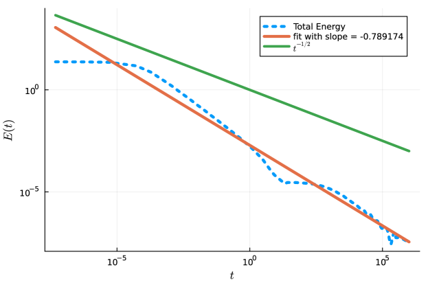
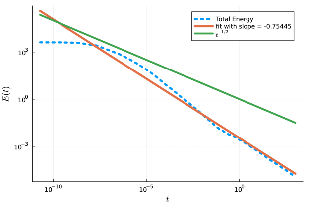
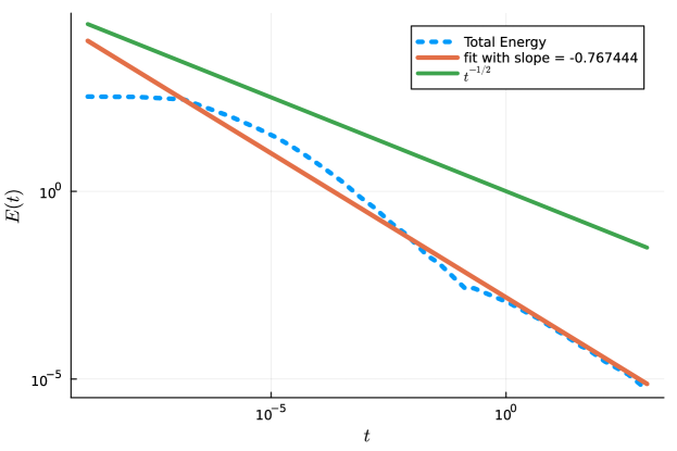
In all tests, we compare the decay rate of the total energy with the theoretical bound $\mathcal{O}(\frac{1}{\sqrt{t}})$ (see equation (8) in the introduction) and provide a best fit line with computed slope given in the legend for each of these decay estimates.

To test the total energy decay, the simulations are run to $T\geq 1e+03$ and the truncation parameter, $L$, may also vary across tests. In every test, $\Delta k_{i}=\Delta k=0.2$ for simplicity. As the theory suggests the decay bound should hold for any finite interval, and as the purpose of the present article is to investigate this, we do not perform an analysis of the truncation parameter’s influence on the solutions, though computational experiments indicate that the influence of $L$ on the current scheme, for the initial distributions considered, is negligible.

Test 1

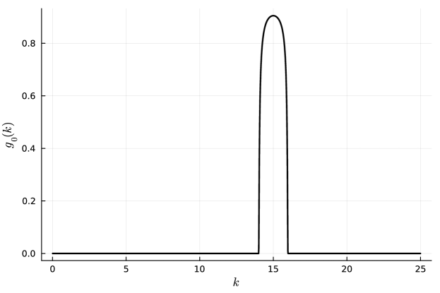
The first example employs an initial distribution which is compactly supported at lower frequencies and given by

$$g(0,k)=\begin{cases}\exp\Big{(}\frac{1}{10(|k-15|^{2}-1)}\Big{)}&\text{if }|k-15|\leq 1\\ 0&\mathrm{otherwise},\end{cases}$$ (32)

as shown in figure 1. Here, as we are interested in the long-time behavior in any finite interval of the wave-number domain, the truncation parameter is set to $L=30$. Larger values of the truncation parameter are used in subsequent tests.

In Figure 2, the total energy is plotted against the theoretical rate. The plot indicates that the total energy in the finite interval considered is conserved for a short time, as shown in [27]. After this time, the total energy in the interval begins to decay rapidly. Interestingly, it would appear that the total energy is again conserved for a short time before decaying again at a slower rate that more closely matches the theoretical bound. Similar behavior is observed for the other initial conditions considered. We provide a best fit line to the total energy data, which shows that the long-time decay rate for the total energy is indeed bounded by the theoretical rate as the reported slope is less than that of the theoretical rate bound.

Figure 1: Initial condition corresponding to equation (32).

Figure 2: Decay rate of total energy corresponding to (32) with theoretical rate, $t^{-\frac{1}{2}}$, shown for reference.

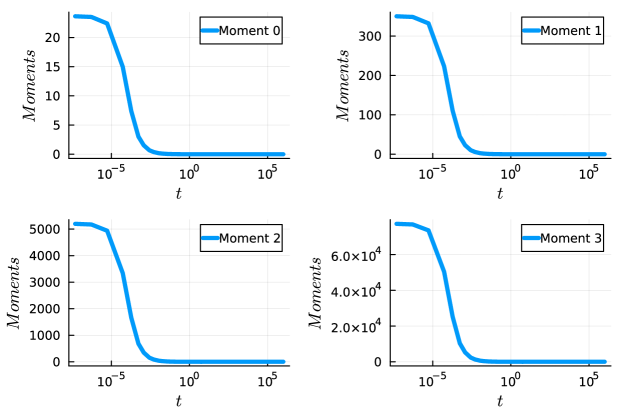
Figure 3: Moments of the energy density for initial condition (32).

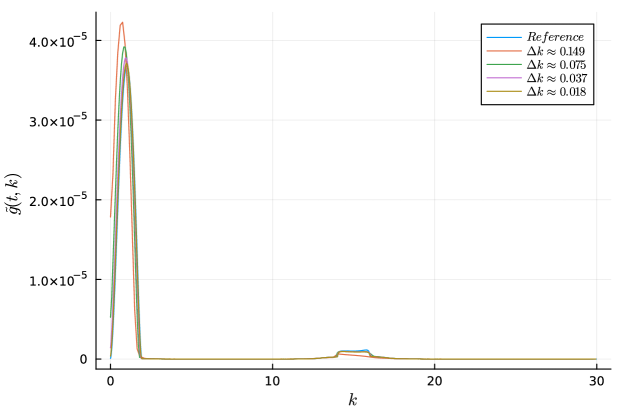
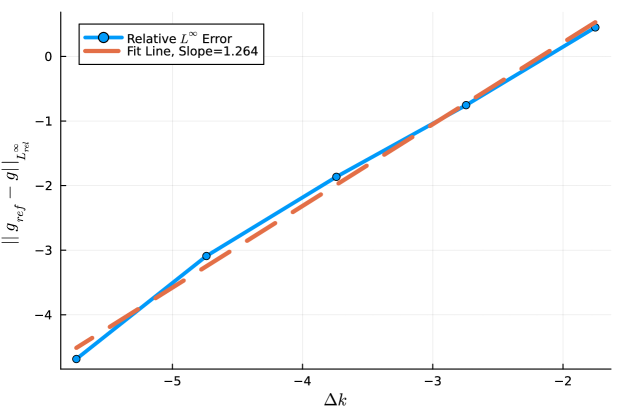
For this initial condition, we present an empirical convergence analysis. Convergence is measured with respect to a fine grid solution with $3200$ cells. For the convergence analysis, we keep $L=30$ and run until $T=10$. See Figure 4 for the results. The plot shows the relative $L^{\infty}([0,L])$ norm of the computed solution with the fine grid solution. A best fit line is shown with computed slope given in the plot legend.

Further, we provide computed convergence rates in table 2 where the convergence rates are computed with the formulas [45]

$$p\approx\log_{2}(E_{\Delta k}/E_{\Delta k/2}-1),$$ (33)

and

$$p\approx\log_{2}(\tilde{E}_{\Delta k}/\tilde{E}_{\Delta k/2}),$$ (34)

with $E_{\Delta k}=\frac{\|g_{\Delta k}-g_{\Delta k/4}\|_{L^{\infty}([0,L])}}{\|g_{\Delta k/4}\|_{L^{\infty}([0,L])}}$ and $\tilde{E}_{\Delta k}=\frac{\|g_{\Delta k}-g_{\Delta k/2}\|_{L^{\infty}([0,L])}}{\|g_{\Delta k/2}\|_{L^{\infty}([0,L])}}$. The results in table 2 show that the approximate rates from both formula (33) and (34) are consistent with each other and the plotted convergence results in figure 4. In figure 5, we see the computed output from method (29) for successively refined grids at time $T=10$ as stated previously. We see the solution has a small jump at the location of the initial distribution (see figure 1) which may explain the first order convergence. Indeed from the coarsest grid, the jump discontinuity is not resolved which explains the higher convergence rates for the coarser grid in table 2. However, the result is positive since we do not preclude discontinuous distributions and we see optimal convergence of the scheme for this discontinuous solution.

Figure 4: Convergence study with initial distribution (32). The cell length is halved in each successive run. Computed solutions use $\Delta k$ values of approximately $0.297$, $0.149$, $0.075$ and $0.037$ above. Shown is a log-log plot of the convergence study results. A best fit line is shown with computed slope given in the legend.

$\Delta k$	$p\approx\log_{2}\left(\frac{E_{\Delta k}}{E_{\Delta k/2}}-1\right)$	$p\approx\log_{2}\left(\frac{\tilde{E}_{\Delta k}}{\tilde{E}_{\Delta k/2}}\right)$
0.2970	1.3334	1.2324
0.1493	1.0138	1.0812
0.0748	1.0002	0.9848
0.0375	1.0138	1.0035

Table 2: Computed convergence rates using formula (33) in the first column and formula (33) in the second column.

Figure 5: Successively refined solutions plotted against a reference solution with 3200 cells at time $T=10$.

Test 2

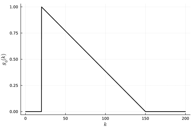
For our second example, we initialize the solver with a discontinuous distribution that has support ranging from low wavenumbers to higher wavenumbers as depicted in Figure 6 and given in equation (35) below,

$$g(0,k)=\begin{cases}1-\frac{1}{130}(k-20)&\text{if }20\leq k\leq 150\\ 0&\mathrm{otherwise}.\end{cases}$$ (35)

For this test, the truncation parameter is set to $L=200$ and the simulation is run until $T=1e+03$. In this and the next test, the initial energy density profile is spread throughout the computational domain, increasing the total energy in the interval we consider.

Figure 6: Initial condition corresponding to equation (35).

Figure 7: Decay rate of total energy corresponding to (35) with theoretical rate and best fit line through the data shown for reference.

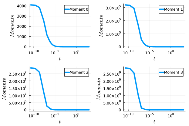
Figure 8: Moments of the energy density for initial condition (35).

Test 3

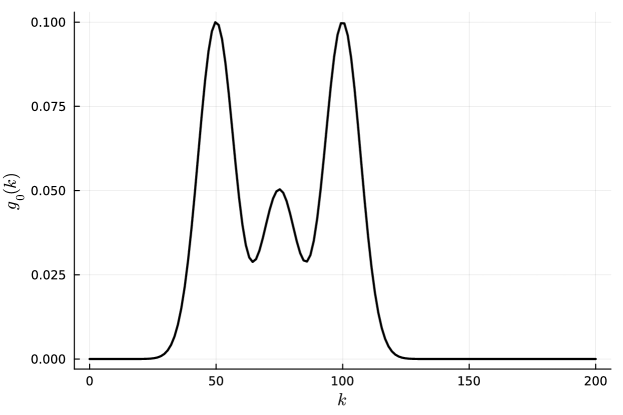
Our last test is depicted in Figure 9 and given by

$$g(0,k)=\frac{1}{10}\Bigg{(}\exp\Big{(}-\frac{(k-50)^{2}}{100}\Big{)}+\frac{1}{2}\exp\Big{(}-\frac{(k-75)^{2}}{100}\Big{)}+\exp\Big{(}-\frac{(k-100)^{2}}{100}\Big{)}\Bigg{)},$$ (36)

for which we employ the same value of the truncation parameter as in the preceding test, $L=200$, and run until $T=1e+03$ once more. The total energy is shown in figure 10. Again, we see that there is good agreement with the theoretical bound and the computed decay rate.

Figure 9: Initial condition corresponding to equation (36).

Figure 10: Decay rate of total energy corresponding to (36) with theoretical rate and best fit line through the data shown for reference.

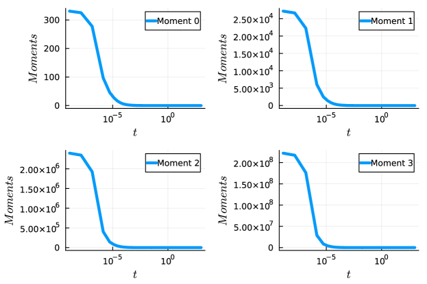
Figure 11: Moments of the energy density for initial condition (36).

5 Conclusions

In this article, we were able to extend the work found in [1] from the simple case when only the forward-cascade part of the collision operator is kept to much more complicated situation when the complete collision operator is treated. A conservative form for the energy density was derived and subsequently an implicit finite volume scheme was given. The implicit finite volume scheme does not suffer from a restrictive stability condition on the time step as is true for the explicit scheme for the forward-cascade equation, which was crucial given the extremely stiff behavior of the complete collision-flux. This was achievable do to a further simplification at the discrete level of the collision-flux. A future work will be dedicated to a 3-WKE tailored time-step control for higher-order time integration to ensure positivity for a given positive initial distribution.

In each numerical test, we verified that the energy was conserved locally in time on the finite intervals we considered and that the theoretical bound (8) was adhered to with similar computed rates across tests. This is in strong agreement with the results found in [27].

References

• [1] S. Walton, T. M.-B., A numerical scheme for wave turbulence: 3-wave kinetic equations, SIAM Journal on Scientific Computing, 45 (4), B467-B492 (2023).
• [2] R. Peierls, Zur kinetischen theorie der warmeleitung in kristallen, Annalen der Physik 395 (8) (1929) 1055–1101.
• [3] R. E. Peierls, Quantum theory of solids, in: Theoretical physics in the twentieth century (Pauli memorial volume), Interscience, New York, 1960, pp. 140–160.
• [4] K. Hasselmann, On the non-linear energy transfer in a gravity-wave spectrum part 1. general theory, Journal of Fluid Mechanics 12 (04) (1962) 481–500.
• [5] K. Hasselmann, On the spectral dissipation of ocean waves due to white capping, Boundary-Layer Meteorology 6 (1-2) (1974) 107–127.
• [6] D. J. Benney, P. G. Saffman, Nonlinear interactions of random waves in a dispersive medium, Proc. R. Soc. Lond. A 289 (1418) (1966) 301–320.
• [7] V. E. Zakharov, V. S. L’vov, G. Falkovich, Kolmogorov spectra of turbulence I: Wave turbulence, Springer Science & Business Media, 2012.
• [8] D. J. Benney, A. C. Newell, Random wave closures, Studies in Applied Mathematics 48 (1) (1969) 29–53.
• [9] S. Nazarenko, Wave turbulence, Vol. 825 of Lecture Notes in Physics, Springer, Heidelberg, 2011. doi:10.1007/978-3-642-15942-8.
URL http://dx.doi.org/10.1007/978-3-642-15942-8
• [10] Y. Pomeau, M.-B. Tran, Statistical physics of non equilibrium quantum phenomena, Lecture Notes in Physics, Springer (2019).
• [11] R. Alonso, I. M. Gamba, M.-B. Tran, The Cauchy problem and BEC stability for the quantum Boltzmann-Gross-Pitaevskii system for bosons at very low temperature, arXiv preprint arXiv:1609.07467 (2016).
• [12] M. Escobedo, M.-B. Tran, Convergence to equilibrium of a linearized quantum Boltzmann equation for bosons at very low temperature, Kinetic and Related Models 8 (3) (2015) 493–531.
• [13] I. M. Gamba, L. M. Smith, M.-B. Tran, On the wave turbulence theory for stratified flows in the ocean, M3AS: Mathematical Models and Methods in Applied Sciences. Vol. 30, No. 1 105-137 (2020).
• [14] T. T. Nguyen, M.-B. Tran, On the Kinetic Equation in Zakharov’s Wave Turbulence Theory for Capillary Waves, SIAM J. Math. Anal. 50 (2) (2018) 2020–2047. doi:10.1137/17M1125042.
URL https://doi.org/10.1137/17M1125042
• [15] T. T. Nguyen, M.-B. Tran, Uniform in time lower bound for solutions to a quantum boltzmann equation of bosons, Archive for Rational Mechanics and Analysis 231 (1) (2019) 63–89.
• [16] B. Rumpf, A. Soffer, M.-B. Tran, On the wave turbulence theory: ergodicity for the elastic beam wave equation, Submitted (2021).
• [17] M.-B. Tran, G. Craciun, L. M. Smith, S. Boldyrev, A reaction network approach to the theory of acoustic wave turbulence, Journal of Differential Equations 269 (5) (2020) 4332–4352.
• [18] C. Collot, H. Dietert, P. Germain, Stability and cascades for the kolmogorov–zakharov spectrum of wave turbulence, Archive for Rational Mechanics and Analysis 248 (1) (2024) 7.
• [19] M. Escobedo, J. J. L. Velázquez, Finite time blow-up and condensation for the bosonic Nordheim equation, Invent. Math. 200 (3) (2015) 761–847. doi:10.1007/s00222-014-0539-7.
URL http://dx.doi.org/10.1007/s00222-014-0539-7
• [20] M. Escobedo, J. J. L. Velázquez, On the theory of weak turbulence for the nonlinear Schrödinger equation, Mem. Amer. Math. Soc. 238 (1124) (2015) v+107. doi:10.1090/memo/1124.
URL http://dx.doi.org/10.1090/memo/1124
• [21] P. Germain, J. La, K. Z. Zhang, Local well-posedness for the kinetic mmt model, arXiv preprint arXiv:2310.11893 (2023).
• [22] P. Germain, A. D. Ionescu, M.-B. Tran, Optimal local well-posedness theory for the kinetic wave equation, Journal of Functional Analysis 279 (4) (2020) 108570.
• [23] A. Soffer, M.-B. Tran, On the dynamics of finite temperature trapped bose gases, Advances in Mathematics 325 (2018) 533–607.
• [24] C. Connaughton, Numerical solutions of the isotropic 3-wave kinetic equation, Physica D: Nonlinear Phenomena 238 (23) (2009) 2282–2297.
• [25] C. Connaughton, P. Krapivsky, Aggregation–fragmentation processes and decaying three-wave turbulence, Physical Review E 81 (3) (2010) 035303.
• [26] C. Connaughton, A. C. Newell, Dynamical scaling and the finite-capacity anomaly in three-wave turbulence, Physical Review E 81 (3) (2010) 036303.
• [27] A. Soffer, M.-B. Tran, On the energy cascade of 3-wave kinetic equations: beyond Kolmogorov–Zakharov solutions, Communications in Mathematical Physics (2019) 1–48.
• [28] N. K. Bell, V. N. Grebenev, S. B. Medvedev, S. V. Nazarenko, Self-similar evolution of alfven wave turbulence, Journal of Physics A: Mathematical and Theoretical 50 (43) (2017) 435501.
• [29] B. V. Semisalov, V. N. Grebenev, S. B. Medvedev, S. V. Nazarenko, Numerical analysis of a self-similar turbulent flow in Bose–Einstein condensates, Communications in Nonlinear Science and Numerical Simulation 102 (2021) 105903.
• [30] T. Buckmaster, P. Germain, Z. Hani, J. Shatah, Effective dynamics of the nonlinear schrödinger equation on large domains, Communications on Pure and Applied Mathematics 71 (7) (2018) 1407–1460.
• [31] T. Buckmaster, P. Germain, Z. Hani, J. Shatah, Onset of the wave turbulence description of the longtime behavior of the nonlinear schrödinger equation, Inventiones Mathematicae 225 (3) (2021) 787–855.
• [32] C. Collot, P. Germain, Derivation of the homogeneous kinetic wave equation: longer time scales, arXiv preprint arXiv:2007.03508 (2020).
• [33] Y. Deng, Z. Hani, Long time justification of wave turbulence theory, arXiv e-prints (2023) arXiv–2311.
• [34] A. Dymov, S. Kuksin, Formal expansions in stochastic model for wave turbulence 1: kinetic limit, arXiv preprint arXiv:1907.04531 (2019).
• [35] Z. Hani, J. Shatah, H. Zhu, Inhomogeneous turbulence for wick nls, arXiv preprint arXiv:2309.12037 (2023).
• [36] H. Spohn, Weakly nonlinear wave equations with random initial data, in: Proceedings of the International Congress of Mathematicians. Volume III, Hindustan Book Agency, New Delhi, 2010, pp. 2128–2143.
• [37] G. Staffilani, M.-B. Tran, On the wave turbulence theory for a stochastic kdv type equation, arXiv preprint arXiv:2106.09819 (2021).
• [38] I. Higueras, Representations of runge–kutta methods and strong stability preserving methods, SIAM Journal on Numerical Analysis 43 (3) (2005) 924–948. doi:10.1137/S0036142903427068.
URL https://doi.org/10.1137/S0036142903427068
• [39] C. Rackauckas, Q. Nie, Differentialequations.jl–a performant and feature-rich ecosystem for solving differential equations in Julia, Journal of Open Research Software 5 (1) (2017) 15.
• [40] J. Bezanson, A. Edelman, S. Karpinski, V. B. Shah, Julia: A fresh approach to numerical computing, SIAM review 59 (1) (2017) 65–98.
URL https://doi.org/10.1137/141000671
• [41] M. Hosea, L. Shampine, Analysis and implementation of tr-bdf2, Applied Numerical Mathematics 20 (1) (1996) 21–37, method of Lines for Time-Dependent Problems. doi:https://doi.org/10.1016/0168-9274(95)00115-8.
URL https://www.sciencedirect.com/science/article/pii/0168927495001158
• [42] S. Dharmaraja, Y. Wang, G. Strang, Optimal stability for trapezoidal–backward difference split-steps, IMA Journal of Numerical Analysis 30 (1) (2010) 141–148. doi:10.1093/imanum/drp022.
• [43] J. D. Edwards, J. E. Morel, D. A. Knoll, Nonlinear variants of the TR/BDF2 method for thermal radiative diffusion, Journal of Computational Physics 230 (4) (2011) 1198–1214. doi:https://doi.org/10.1016/j.jcp.2010.10.035.
URL https://www.sciencedirect.com/science/article/pii/S0021999110005917
• [44] E. Hairer, G. Wanner, S. P. Nørsett, Solving Ordinary Differential Equations I: Nonstiff Problems, 2nd Edition, Springer Series in Computational Mathematics, Springer Berlin, Heidelberg, 1993, hardcover ISBN: 978-3-540-56670-0, Published: 05 August 1993. doi:10.1007/978-3-540-78862-1.
URL https://doi.org/10.1007/978-3-540-78862-1
• [45] R. J. LeVeque, Finite Difference Methods for Ordinary and Partial Differential Equations: Steady-State and Time-Dependent Problems, SIAM, 2007.