Why do Learning Rates Transfer?
Reconciling Optimization and Scaling Limits for Deep Learning

Abstract

Recently, there has been growing evidence that if the width and depth of a neural network are scaled toward the so-called rich feature learning limit ($\mu$P and its depth extension), then some hyperparameters — such as the learning rate — exhibit transfer from small to very large models, thus reducing the cost of hyperparameter tuning. From an optimization perspective, this phenomenon is puzzling, as it implies that the loss landscape is remarkably consistent across very different model sizes. In this work, we find empirical evidence that learning rate transfer can be attributed to the fact that under $\mu$P and its depth extension, the largest eigenvalue of the training loss Hessian (i.e. the sharpness) is largely independent of the width and depth of the network for a sustained period of training time. On the other hand, we show that under the neural tangent kernel (NTK) regime, the sharpness exhibits very different dynamics at different scales, thus preventing learning rate transfer. But what causes these differences in the sharpness dynamics? Through a connection between the spectra of the Hessian and the NTK matrix, we argue that the cause lies in the presence (for $\mu$P) or progressive absence (for the NTK regime) of feature learning, which results in a different evolution of the NTK, and thus of the sharpness. We corroborate our claims with a substantial suite of experiments, covering a wide range of datasets and architectures: from ResNets and Vision Transformers trained on benchmark vision datasets to Transformers-based language models trained on WikiText.

1 Introduction

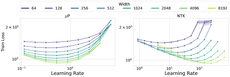
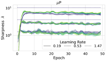
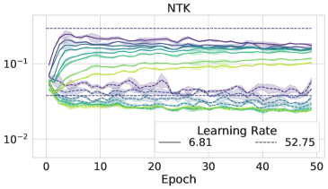
Figure 1: Top row: learning rate transfer for $\mu$P, but not for NTP. Bottom row: sharpness’ dynamics. Notice how the sharpness is width-independent for $\mu$P, but is decreasing in NTP. Also notice how in this case for $\mu$P the optimal learning rate corresponds to a sharpness that is close to EoS (black dashed lines). We argue that a width-independent sharpness is at the hearth of learning rate transfers. The architecture is a two-layer convolutional network trained on CIFAR-10 with data augmentation, where the width corresponds to the number of filters in the convolution. (See App. B). The width in the legend here refers to the size of the final linear readout layer. Other parameters: $B=128$, epochs $=50$.

Recent trends in deep learning research have unmistakably shifted towards an increase in model sizes, with networks comprising of billions of parameters emerging as the standard (Zhao et al., 2023). However, as models enlarge, so does the cost incurred in hyperparameter tuning which has led researchers to look for ways to scale up the architecture — both in terms of width and depth — while preserving the optimal hyperparameters (such as the learning rate).

While there exist several ways to scale up the width and depth of the network, not all of them facilitate learning rate transfer. For standard deep learning practices, such as networks initialized with LeCun/Kaiming techniques (LeCun, 2002, He et al., 2015), a significant shift in the optimal learning rate is usually observed as the width and the depth of the model are increased. Similarly, under the NTK regime Jacot et al. (2018), which provides theoretical insights into the linearized behavior of very wide neural networks during training, the optimal learning rate also varies as the width and depth of the network change. Alternatively, Yang and Hu (2021), Yang et al. (2022) propose the $\mu$P framework, designed to maximize the gradient update of the representations of the intermediate layers (i.e. feature learning) as the width increases. Under $\mu$P scaling, and its depth extension for residual networks $\mu P-\sqrt{\text{depth}}$ (Bordelon et al., 2023, Yang et al., 2023), it has been empirically demonstrated that the learning rate transfers across both width and depth.

From an optimization theory viewpoint, however, the rationale behind the connection between the nature of the scaling limit and learning rate transfer remains unclear. In the theory of smooth convex (Nesterov, 2013), nonconvex (Garrigos and Gower, 2023), and stochastic (Gower et al., 2019) optimization, the sharpness — i.e. the maximum Hessian eigenvalue — plays a crucial role in the selection of the optimal step size, and in the guarantees of convergence of gradient methods. As the Hessian dynamics are in general dependent on the network’s width and depth, it is not obvious why the optimal learning rate of a small model should transfer to a larger one.

In this paper, we bridge the gap between the nature of the scaling limit and the loss landscape by comparing the NTK and $\mu$P regimes. We unveil the surprising fact that for $\mu$P and its depth extension, the sharpness remains largely independent of the width and depth of the network. Instead, it progressively converges to a threshold mostly dependent on the batch size and learning rate, which in some cases corresponds to the Edge of Stability (EoS) value (Cohen et al., 2021). Once the sharpness converges to this threshold, it oscillates around it for a sustained period of training time, maintaining dynamics which are largely width/depth-independent. On the other hand, we show that under the NTK regime, the sharpness dynamics significantly separate during training for different widths. Small-width models are still converging to the limiting threshold, while larger width models progressively slow down their convergence. More concretely:

• We show that under $\mu$P, after a progressive sharpening phase, the dynamics of the largest Hessian eigenvalue $\lambda$ stabilize to a width-independent value (Fig. 1, top left). This correlates with the phenomenon of hyperparameter transfer (Fig. 1, bottom left) as expected by optimization theory. On the other hand, we show in Fig. 1 (right column) that this is not the case for the NTK regime, where the sharpness is decreasing in width. Also, here we do not observe learning rate transfer.

• Thanks to the depth extension $\mu$P $-\sqrt{\text{depth}}$, we show that our observations remain valid when the depth is scaled up, testing networks with up to $200$ layers.

• We show that the results on width/depth-independent sharpness are consistent at realistic scale, including ResNets and Vision Transformers (ViTs) trained on Imagenet and GPT-2 on text data.

• We investigate the threshold that is reached during the progressive sharpening phase (in $\mu$P), connecting our findings to the line of work of Edge of Stability Cohen et al. (2021). In particular, EoS is achieved width/depth-independently for large batch sizes and relatively large learning rates, while for small batches the sharpness stays below EoS (while still being largely independent of the width/depth).

These results on width/depth-independent sharpness provide a clean interpretation for learning rate transfer: under $\mu$P, the key landscape features along the trajectory of gradient descent are remarkably similar across different scales. But why does this hold only for $\mu$P but not for the neural tangent parameterization (NTP) or other initialization/parameterization strategies? We argue that while in $\mu$P feature learning guarantees progressive sharpening to reach a width-independent sharpness at any scale, in NTP the progressive lack of feature learning when the width is increased prevents the Hessian from adapting, and its largest eigenvalue from reaching the convergence threshold. More concretely, in Section 3.1 we show that the progressive sharpening phase is mainly driven by the evolution of the NTK’s largest eigenvalue, which is asymptotically fixed to its initial value for NTP, while it evolves at any width under $\mu$P. This disparity elucidates the distinct behaviors of sharpness under these parameterizations, shedding light on the intricate interplay between scaling limits and optimization dynamics. We hope that our results help reduce conceptual gaps between the lines of research on scaling limits and optimization.

The rest of the paper is organized as follows. In Section 2 we provide the necessary background on scaling limits, optimization of neural networks, and EoS. In Section 3 we present the main empirical results on the connection between sharpness and hyperparameter transfer while in Section 4 we provide further intuition with a theoretical analysis on a two-layer linear network. Finally, in Section 5 we discuss the relevance of our results in the existing literature and conclude with potential future directions. We defer a more extensive discussion on related work to the appendix (Sec. A).

2 Background

2.1 Scaling Limits of Neural Networks

We consider a neural network with residual connections, defined by the following recursive equations over the layer indexes $\ell\in[L]$:

$$h^{\ell+1}(x)=h^{\ell}(x)+\frac{1}{\sqrt{N}L^{\alpha}}W^{\ell}\phi(h^{\ell}(x)),$$ (1)

where $N$ and $L$ are the width and depth of the network, $W^{\ell}\in\mathbb{R}^{N\times N}$ for $\ell=1,\dots,L-1$. We denote the output with $f(x)=\frac{1}{\gamma}W^{L}\phi(h^{L}(x))$, where $W^{L}\in\mathbb{R}^{1\times N}$ and $\gamma$ scales the network output and has a crucial role on transfer. Similarly, $\alpha$ has the role of interpolating between different depth limit regimes. At the first layer, we define $h^{1}(x)=\frac{1}{\sqrt{D}}W^{0}x$, where $W^{0}\in\mathbb{R}^{N\times D}$. All the weights $\theta=\{W^{\ell}\}_{l=0}^{L}$ are initialized independently from $\mathcal{N}(0,1)$ and we denote with $P$ the total number of parameters. We stress that the fully connected layer can be replaced with any type of layer (our experiments include convolutional and attention layers). Given a dataset $\mathcal{D}=\{(x_{\mu},y_{\mu})\}_{\mu=1}^{|\mathcal{D}|}$ of datapoints $x_{\mu}\in\mathbb{R}^{D}$ and labels $y_{\mu}\in\mathbb{R}$, we train the network with stochastic gradient descent (SGD) with batch size $B$ and learning rate $\eta\in\mathbb{R}$:

$$\theta_{t+1}=\theta_{t}-\eta\sum_{\mu=1}^{B}\nabla_{\theta}\mathcal{L}(f_{t}(x_{\mu}))$$ (2)

where $\mathcal{L}$ is a twice differentiable loss function. Defining $f_{t}:=(f_{t}(x_{\mu}))_{\mu\in[|\mathcal{D}|]}\in\mathbb{R}^{|\mathcal{D}|}$ to be the vector of network’s outputs at time $t$, if one considers continuous time, the corresponding gradient descent dynamics in function space $df_{t}/dt$ take the following form Arora et al. (2019):

$$\frac{df_{t}}{dt}=-\Theta(f_{t})\Delta(f_{t}),$$ (3)

where $\Delta(f_{t})_{i}:=\partial{\mathcal{L}(f_{t}(x_{i}))}/\partial f_{t}(x_{i})$, $i\in[|\mathcal{D}|]$ is the vector of residuals, and

$$\Theta(f_{t})_{ij}:=\langle\nabla_{\theta}f_{t}(x_{i}),\nabla_{\theta}f_{t}(x_{j})\rangle$$ (4)

for $i,j\in[|\mathcal{D}|]$ is the neural tangent kernel (NTK).

Infinite Width.

The parameters $\gamma,\alpha,\eta\in\mathbb{R}$ determine the nature of the scaling limit. If $\gamma=\gamma_{0},\eta=\eta_{0}$ are $\mathcal{O}(1)$ constants with respect to $N,L$ (neural tangent parameterization, or NTP), then the network enters the NTK regime Jacot et al. (2018). Here, in the limit of infinite width, the NTK remains constant to its value at initialization throughout training, i.e. $\Theta(f_{t})=\Theta(f_{0})$ for all $t\geq 0$. Thus, the network’s dynamics become equivalent to a linear model trained on the first order term of the Taylor expansion of the model at initialization Lee et al. (2019). The fact that the NTK is fixed to its value at initialization is associated with the lack of feature learning of the model in the large width limit.

If $\gamma=\gamma_{0}\sqrt{N}$, and $\eta=\eta_{0}\gamma^{2}$ ($\mu$P, or mean-field parameterization), the features evolve in the limit (i.e. the NTK $\Theta(f_{t})$ evolves), and the richer model’s dynamics can be described using either Tensor Programs Yang and Hu (2021) or dynamical mean field theory Bordelon and Pehlevan (2022). Under $\mu$P, Yang et al. (2022) show that hyperparameters transfer across width, in contrast to kernel limits, which we reproduce for our residual network in Fig. 1.

Infinite Depth.

If on top of the $\mu$P framework, the residual branches are scaled with $\alpha=1/2$ ($\mu$P-$\sqrt{L}$ parameterization), then Bordelon et al. (2023) and Yang et al. (2023) show that the infinite width dynamics also admit a feature-learning infinite depth limit. Under $\mu$P-$\sqrt{L}$, the learning rate transfers with both width and depth. In this paper, we compare NTP and $\mu$P regimes as the width is increased, and show that our results extend to depth-scaling using the $\mu$P-$\sqrt{L}$ model.

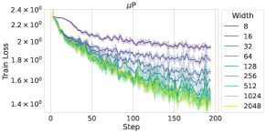
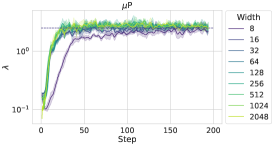
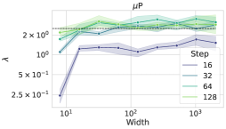
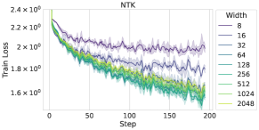
() Loss curves

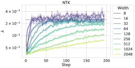
() Sharpness dynamics

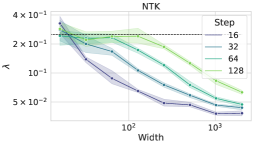
() Sharpness vs width

Figure 2: Early training dynamics in $\mu$P (top row) and NTP parameterization (bottom row). (a) Loss curves. (b): Sharpness dynamics. Notice how for $\mu$P progressive sharpening until EoS (black dashed line) is achieved at any width and with comparable speed, while for NTP the time to EoS progressively increase with width. Also, the loss curves start to depart from each other as training progresses, while $\lambda$ stays at EoS for a more sustained period ot time. (c) Sharpness vs width at selected time steps. For $\mu$P, $\lambda$ converges very fast in width, while in NTP it diminishes. Other parameters: architecture: Three-layer convolutional network. Dataset: CIFAR-10, without data augmentation. $B=128$, epochs $=1$, learning rate $\eta_{0}=0.8$ for $\mu$P and $8$ for NTP. The reported width is the size of the readout layer.

2.2 Conditions for hyperparameter transfer

The empirical success of hyperparameter transfer crucially relies on the following two observations/desiderata.

1. The optimal learning rate is consistent across widths/depths (hyperparameter transfer).

2. The models show consistent improvement in training speed with respect to the scaling quantity (i.e. there is a clear “wider/deeper is better” effect), indicating that the loss dynamics have not yet converged to the limiting behaviour predicted by the theory.

From these observations, we conclude that transfer does not necessarily imply matching loss dynamics. In this paper, we argue that there are instead properties of the loss landscape along the SGD trajectory that effectively transfer in a largely width/depth independent way under the right scaling of the architecture. Thus, the optimal learning rate is preserved across width/depth throughout a sizeable fraction of the training trajectory.

2.3 Optimization: Optimal Learning Rate and Edge of Stability

We analyze the sharpness $\lambda_{t}$, defined as the largest eigenvalue of the Hessian: $\nabla^{2}_{\theta}\mathcal{L}(\theta_{t}):=\sum_{\mu}\nabla^{2}_{\theta}\mathcal{L}(f_{t}(x_{\mu}))\in\mathbb{R}^{P\times P}$, as $\theta_{t}$ evolves with gradient descent. There are an abundance of works in the literature that have studied the structure of the Hessian in deep models (Singh et al., 2021, Martens, 2020, Orvieto et al., 2021). The sharpness has been linked to various aspects of training speed and stability, and often provides a theoretically principled upper bound on the maximum step size allowed. For instance, for a quadratic objective, $\lambda_{t}=\lambda$ is constant and gradient descent would diverge if the learning rate $\eta>2/\lambda$, and training speed is maximized for $\eta=1/\lambda$ (LeCun et al. (2002), page 28). Beyond this classical example, the descent lemma (Nesterov, 2013) states that for a general non-convex loss $\mathcal{L}$,

$$\mathcal{L}(\theta_{t+1})-\mathcal{L}(\theta_{t})\leq-\left(\eta-\frac{\eta^{2}\lambda_{t}}{2}\right)\|\nabla\mathcal{L}(\theta_{t})\|^{2}.$$

The lemma predicts that $\mathcal{L}(\theta_{t+1})-\mathcal{L}(\theta_{t})$ if $\eta\leq\frac{2}{\beta}$ where $\beta:=\sup_{\theta}\|\nabla^{2}L(\theta)\|_{2}$, where $\|\nabla^{2}L(\theta)\|_{2}$ is the sharpness at $\theta$. When it comes to deep neural networks, $\lambda_{t}$ is generally observed to increase during training (progressive sharpening): in the early phase of training it increases Jastrzkebski et al. (2018), Jastrzebski et al. (2020) (depending on the learning rate and the batch size) and then it decreases close to convergence Sagun et al. (2016). Under full batch gradient descent training, the sharpness consistently rises above the Edge of Stability (EoS) threshold of $2/\eta$.

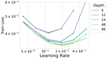
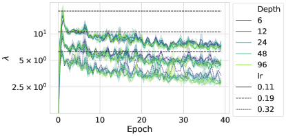
Figure 3: Depth-extension on ResNet (Eq. 1) with convolutional layers and ReLU activation trained on CIFAR-10 for 80 epochs (with data augmentation). The bottom plot shows the sharpness for the first 40 epochs of training. The width is fixed at 128.

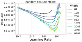
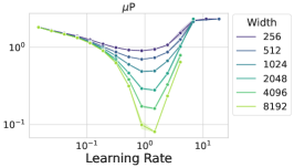
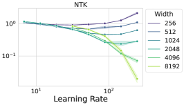
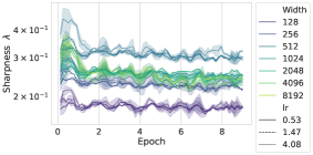
() Random Features

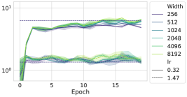
() $\mu$P

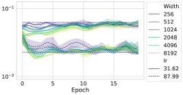
() NTP

Figure 4: Learning rate transfer plot (top row) and sharpness dynamics (bottom row) for a three-layer convolutional network and three different settings. (a) random feature model (only the readout layer is trained), (b) and (c) correspond to $\mu$P and NTP parameterizations, respectively. In random feature learning, the absence of feature learning prevents the sharpness’ evolution at any width, thus learning rate transfer coincides with the convergence of the sharpness $\lambda$ at initialization. Also notice how for NTP, the progressive sharpening converges to $\lambda=2/\eta_{0}$ at a much lower speed as the width increases, in line with the early dynamics reported in Fig. 2. Other parameters: $B=128$, epochs $=20$ for the $\mu$P/NTP models and $10$ for the random feature model, dataset: CIFAR-10, without data augmentation.

3 Why Do Learning Rates Transfer?

Motivated by the intrinsic dependencies between the sharpness $\lambda$ and optimal learning rate, we study the time evolution of $\lambda$ as a function of width and observe the following:

Observation 1: in $\mu$P (and $\mu$P-$\sqrt{L}$), optimization happens along trajectories of $N,L-$independent sharpness $\lambda$, while for NTP the sharpness decreases in width.

We remark that under the observation that the sharpness $\lambda$ controls the maximum step size allowed, having $N,L$-independent trajectories provides supporting evidence for learning rate transfer, as the optimal learning rate will also be $N,L$-independent.

In Fig. 1 we train a two-layer convolutional network under the $\mu$P and NTP scalings with cross entropy loss, while keeping track of the sharpness at fixed gradient step intervals. The top row shows the dynamics of $\lambda$. Notice how the sharpness’ behaviour is qualitatively different in the two parameterizations: in $\mu$P it reaches a width-independent value which is close to the stability threshold of $2/\eta_{0}$. On the other hand, in NTP we observe a progressive diminishing of the sharpness with width, as previously observed for Mean-Square-Error loss by Cohen et al. (2021).

We then study the effect of depth under the $\mu$P-$\sqrt{L}$ model of Eq. 1. In Fig. 3, we show that the sharpness’ dynamics are also extremely consistent across depth, although progressively diminishing from the EoS threshold. This suggests that EoS is not necessary for the learning rate to transfer, but the consistency of the sharpness’ dynamics is.

$\boldsymbol{N,L}$-independence of the sharpness and loss curves.

In order to have meaningful learning rate transfer (as described in the desiderata in Sec. 2.2), it is necessary that the dynamics of the sharpness stay $N,L$-independent along large parts of the training trajectory, while the higher capacity models (larger width) are able to fit data faster. In other words, $\lambda$ must converge faster than the predictor $f(x)$ with respect to the scaling quantity (width or depth) at any time step. Indeed, this is what we observe:

Observation 2: in $\mu$P (and $\mu$P-$\sqrt{L}$), the $N,L$-independent sharpness is sustained for a long period of training time, while the loss curves progressively depart from each other. In NTP, the sharpness shows inconsistent dynamics from early stages of training.

While the observation of a consistent sharpness at a large time scale can already be observed in Fig. 4 (bottom row), we now directly compare loss curves with sharpness dynamics under $\mu$P and NTP. In Fig. 2, we study the early training dynamics (first 200 gradient steps) of a 3-layer convolutional network under $\mu$P and NTP. Notice how for $\mu$P: (1) the training curves progressively depart from each other — with wider being better — while (2) the sharpness stays at its EoS value of $2/\eta_{0}$ for a sustained period of the training trajectory. Also, notice $\lambda$ reaches the EoS value very consistently in width (only the width 8 model shows slower convergence). On the other hand, under the NTP parametrization, the sharpness decreases in width, and its progressive sharpening phase converges to EoS at different speeds, with shallower models converging faster.

The observation that sharpness dynamics exhibit greater consistency compared to loss dynamics suggests that under $\mu$P scaling, although models with larger capacity fit the data faster, the paths taken by various models through the optimization landscape show a surprisingly uniform curvature.

3.1 Feature Learning and Progressive Sharpening

Observations 1 and 2 provide empirical evidence as to why — from an optimization perspective — $\mu$P exhibits learning rate transfer. Along the lines of Yang et al. (2023) and Bordelon et al. (2023), but with the additional insights from our experiment, we conjecture that under NTP the progressive lack of feature learning and the convergence of the model to its linearization prevents the progressive sharpening needed to reach a $N,L$-independent $\lambda$. By increasing the learning rate $\eta_{0}$, however, the convergence speed to the infinite width limit slows down Lee et al. (2019), and thus larger width networks effectively learn features. This causes the incremental shift of optimal learning rate, as we observe in Figures 1 and 4. This brings us to the conjecture that a feature learning limit is necessary for hyperparameter transfer in deep neural networks.

Indeed, the connection between feature learning and progressive sharpening becomes evident when studying the relationship between the sharpness and the largest eigenvalue of the NTK matrix. Following the Gauss-Newton decomposition Martens (2016; 2020), the Hessian can be decomposed as a sum of two matrices $H=\mathcal{G}+\mathcal{R}$, where $\mathcal{G}$ is the Gauss-Newton (GN) matrix and $\mathcal{R}$ depends on the Hessian of the model. For MSE loss,

$$\mathcal{G}=\sum_{i=1}^{|\mathcal{D}|}\nabla_{\theta}f(x_{i})\nabla_{\theta}f(x_{i})^{\top}=K^{\top}K.$$

where $K\in\mathbb{R}^{|\mathcal{D}|\times P}$ is a matrix where each row is $\nabla_{\theta}f(x_{i})$ (i.e. the Jacobian of $f(x_{i})$), and:

$$\mathcal{R}=\sum_{i=1}^{|\mathcal{D}|}\nabla_{\theta}^{2}f(x_{i})(y_{i}-f(x_{i})),$$

where $y_{i}\in\mathbb{R}$ is the label. One can readily see that the NTK matrix in Eq. 4 can be written as $\Theta(f_{\theta})=KK^{\top}$. Thus, we can immediately see that the NTK and $\mathcal{G}$ share the same nonzero eigenvalues, and in particular the same sharpness ($\lambda(\Theta)=\lambda(\mathcal{G})$). In Figure 5, we show that under $\mu$P the sharpness evolution is dominated by the $\mathcal{G}$ consistently across different widths, while for NTP the sharpness evolution slows down when increasing the width. Since in the limit the NTK matrix is fixed for NTP, while it evolves with time for $\mu$P, these results provide further supporting evidence for the role of feature learning in the evolution of the hessian, and thus in hyperparameter transfer. While this argument strictly holds for MSE loss, it can be generalized to any twice differentiable loss function, albeit with some caveats. In Appendix D, we generalize the setting, analyze the cross-entropy loss and perform validating experiments, confirming the conclusions drawn here.

To test this conjecture further, we compare the NTP and $\mu$P parametrizations to a random feature model, i.e. a model where we all the weights of the intermediate layers are frozen to their value at initialization, and only the final readout layer is trained. Crucially, this model does not learn features by construction for any learning rate and any width. The results are shown in Fig. 4. Notice how the transfer in the random feature model is achieved only at very large widths compared to $\mu$P. However, the transfer is better than in NTP. This is in line with our claim, as under a random feature model increasing the learning rate does not induce more feature learning, as is the case in NTP.

In Section 4 we revisit the above claims more precisely in a simplified setting, providing further intuition on the sharpness dynamics and learning rate transfer.

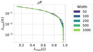
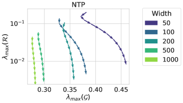
Figure 5: Evolution of the top eigenvalues of the Hessian components $\mathcal{G}$ and $\mathcal{R}$ for a two-layer linear network trained on random data under MSE loss. The vector field characterizes the evolution during training for a fixed learning rate. Left: $\mu$P. Note that all the curves follow the same trajectory and begin with a sharpening phase, after which the residual continues to decrease. Right: NTP. For wider networks the sharpening phase reduces, since the network is approaching the limit where the NTK is fixed to its value at initialization.

3.2 Other experiments

Large scale experiments.

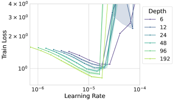
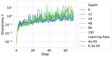
Figure 13: Vision transformers (ViTs) trained on CIFAR10 with Adam. Left figure shows the learning rate transfers across depth in ResNets parameterized with Depth$-\mu$P. Right figure shows that for a fixed learning rate, the sharpness becomes depth independent during training. Parameters: batch size $64$, epochs $10$

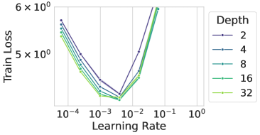
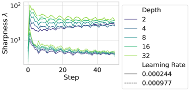
Figure 14: GPT-2 model (encoder only) trained on Wikitext for next-token-prediction using Adam, parameterized with Depth$-\mu$P. Left figure shows the learning rate transfers across depth in text transformers parameterized with Depth$-\mu$P. Right figure shows that for a fixed learning rate, the sharpness becomes depth independent during training. Parameters: batch size $20$, epochs $10$, sequence length $35$, base width $128$.

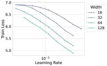
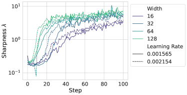
Figure 15: Residual convolutional networks (ResNets) trained on ImageNet with stochastic gradient descent. Left figure shows the learning rate transfers across width in ResNets parameterized with $\mu$P. Right figure shows that for a fixed learning rate, the sharpness becomes width independent during training. Parameters: batch size $128$, epochs $1$.

In App. E.3, (Figures 11, 12, 13, 14, 15) we perform more experiments to validate the connection between the consistency of the sharpness’ dynamics and learning rate transfers across datasets (Tiny-ImageNet, WikiText), architectures (ViT, GPT-2 Radford et al. (2019)), and optimizers (Adam Kingma and Ba (2014)). We find these results to be consistent with those in the main text.

End of training dynamics.

In App. E.1 (Fig. 8), we study the width dependence of the sharpness at the late phase of training. It is well-known that for cross-entropy loss, a phase transition happens where the sharpness starts to decrease Cohen et al. (2021). We found that even for $\mu$P this transition point is width-dependent, with a consequent slight shift in optimal learning rates during this late phase. Again, these results are in line with our results that width-independent sharpness facilitates transfer.

Batch size ablation.

We repeat the experiment in Fig. 1 with increasing batch size, observing that the width-independent threshold is reached across all the tested batch sizes, thus not affecting learning rate transfers. For larger batches, a close-to-EoS threshold is reached across more learning rates. Results are summarized in Fig. 9 and 10 in App. E.2.

4 Case study: Two-Layer Linear Network

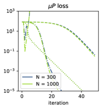
Figure 6: Evolution of loss under $\mu P$ and NTP for the toy example of Section 4: $\frac{1}{2}\|\frac{1}{\sqrt{ND}\gamma}EV-w_{*}\|^{2}$, where $w_{*}=1\in\mathbb{R}^{D}$, $D=100$. This is a minimal example of transfer captured by our theory: $\mu P$ trajectories align. Different linestyles correspond to different values of $\eta_{0}$ (grid is different for $\mu P$ and NTP).

In this section, we revisit and validate our intuition and empirical findings in Sec. 3 through the lens of a two-layer neural network with linear activations and $L2$ loss. Our purpose is to characterize the dynamics of $\mu P$ and NTP at the edge of stability through the lens of a simple example that shares a similar phenomenology with the more complex scenarios observed in the last section (see Fig. 6, App. C). Our setting is similar to the one leading to the insightful analysis of Edge of Stability in Kalra et al. (2023), Song and Yun (2023). Compared to these works, we do not limit the analysis to a single datapoint or to vanishing targets .

Notation and assumptions.

Consider a dataset of $|\mathcal{D}|$ datapoints in $D$ dimensions $X\in\mathbb{R}^{|\mathcal{D}|\times D}$ ($|\mathcal{D}|\geq D$), and labels generated through a latent ground-truth vector $w_{*}\in\mathbb{R}^{D}$, that is $Y=Xw_{*}$. The neural network we use here is parametrized by weights $W^{0}\in\mathbb{R}^{D\times N}$, $W^{1}\in\mathbb{R}^{N\times 1}$, where $N$ is the width. To simplify the notation in our setting, we name $E:=W^{0}$ and $V:=W^{1}$: $f(X)=\frac{1}{\gamma\sqrt{ND}}XEV$, $\mathcal{L}(E,V)=\frac{1}{2}\|f(X)-Y\|^{2}$. We initialize each entry of $E,V$ i.i.d. Gaussian with mean zero and variance $1$. Recall that $\gamma_{\text{\tiny NTP}}=1$, $\gamma_{\text{\tiny$\mu P$ }}=\sqrt{N}$. We train with gradient descent (GD) with a learning rate $\eta=\eta_{0}\gamma^{2}$. Empirically, we observed (Fig. 6, App. C) that picking $|\mathcal{D}|=D$ and data $X=I_{D}$ ($I_{D}$ is the $D\times D$ identity matrix) is sufficient to track most of the crucial features of $\mu P$/ NTP explored in this paper, except the “wider is better” effect which here is less apparent due to the simple hypothesis class. Note that in this setting $|\mathcal{D}|$ cancels and $XE=E$. Thus, $E$ can be interpreted as the matrix of features after the first layer. The loss function reduces to

$$\mathcal{L}(E,V)=\frac{1}{2}\left\|w-w_{*}\right\|^{2},\quad\text{with}\quad w:=\frac{1}{\gamma\sqrt{ND}}EV.$$ (5)

Hessian top eigenvalue, GN and NTK.

Note that using a learning rate $\eta_{0}\gamma^{2}$ when optimizing $\mathcal{L}$ is equivalent to using a learning rate $\eta_{0}$ when optimizing $\gamma^{2}\mathcal{L}$. We now derive closed-form expressions for metrics on $\nabla^{2}\mathcal{L}$. Define

$$e:=\frac{1}{ND}EE^{\top}\in\mathbb{R}^{D\times D},\ \ v:=\frac{1}{ND}V^{\top}V\in\mathbb{R}_{\geq 0}.$$ (6)

The following bound leverages a Gauss-Newton decomposition and leads analytical insights supporting Sec. 3.1.

Lemma 4.1 (GN bound).

Let $\gamma^{2}\nabla^{2}\mathcal{L}=\mathcal{G}+\mathcal{R}$ be Gauss-Newton decomposition (see Sec. 3.1) of the Hessian for the loss in Eq. 5, with $\mathcal{G}=K^{\top}K$, where $K\in\mathbb{R}^{D\times(ND+N)}$.
Let us denote the NTK matrix $\Theta=KK^{\top}\in\mathbb{R}^{D\times D}$. Then

$$\Theta(E,V)=e+v\cdot I_{D}$$

and

$$|\lambda_{\max}[\gamma^{2}\nabla^{2}\mathcal{L}(E,V)]-\lambda_{\max}[\Theta(E,V)]|\leq\sqrt{\frac{\gamma}{ND}}\|w-w_{*}\|_{2}.$$

The result above is actually more general: it indicates that the eigenvalues of the positive semidefinite portion of the Hessian $\mathcal{G}=K^{\top}K$ are fully characterized by the eigenvalues a smaller matrix $\Theta=KK^{\top}$. Furthermore, in our model $\Theta$ has a closed form that depends only on the variables $e,v$. In the next subsection, we characterize how $e,v$ evolve through time, and give conclusions for $\mu$P in Sec. 4.3.

4.1 Dynamics and Edge of Stability in Latent Space

In Sec. 4.3, we show at any value of the width $N$, under GD on the original network parameters $(E,V)$, the dynamics of $w,e,v$, can be described completely through a self-contained dynamical system in $(1+D+D^{2})$ dimensions. This property is surprising because the original dynamical system described by GD on the variables $E,V$ lives in $N(D+1)$ dimensions. Concretely, this means we can study the Hessian dynamics at different network widths in the same space. This result differs significantly in nature from the DMFT equations in (Bordelon and Pehlevan, 2022), where objects evolving are width dependent (evolving objects are features at different layers).

Theorem 4.2 (Evolution Laws).

Let $(E,V)$ evolve with GD at stepsize $\eta=\eta_{0}\gamma^{2}$ on the loss of Eq. 5. The evolution of $(w,e,v)$ is completely described by the following self-contained equation: let the ⁺ denote updated quantities,

$$w^{+} =w-\eta_{0}(v\cdot I_{D}+e)(w-w_{*})+\frac{\eta_{0}^{2}\gamma^{2}}{ND}(ww^{\top}-w_{*}w^{\top})(w-w_{*}).$$

$$e^{+} =e+\frac{\eta_{0}\gamma^{2}}{ND}\left[-2ww^{\top}+w_{*}w^{\top}+ww_{*}^{\top}\right]+\frac{\eta_{0}^{2}\gamma^{2}}{ND}\left[vww^{\top}-vw_{*}w^{\top}-vww_{*}^{\top}+vw_{*}w_{*}^{\top}\right].$$

$$v^{+} =v+\frac{\eta_{0}\gamma^{2}}{ND}\left[-2w^{\top}w+2w_{*}^{\top}w\right]+\frac{\eta^{2}_{0}\gamma^{2}}{ND}\left[w^{\top}ew-2w_{*}^{\top}ew+w_{*}^{\top}ew_{*}\right].$$

While the system above describes the evolution laws $(w_{k},e_{k},v_{k})\to(w_{k+1},e_{k+1},v_{k+1})$, the dynamics are influenced also by initialization.

Proposition 4.3.

At initialization, as $N\to\infty$, $e\overset{\mathbb{P}}{\to}e^{\infty}:=\frac{1}{D}I_{D}$ and $v\overset{\mathbb{P}}{\to}v^{\infty}:=\frac{1}{D}$. Moreover, errors from $\infty-$ initialization scale as $\frac{1}{\sqrt{N}}$ in expectation: $\mathbb{E}|v-v^{\infty}|^{2},\mathbb{E}|e_{ij}-e^{\infty}_{i,j}|^{2}\leq\frac{2}{ND},\ \forall i,j\in[D]$. While for $\gamma=1$ (NTP) $w$ at initialization is in the limit Gaussian with elementwise variance $1/D$, for $\gamma=\sqrt{N}$ ($\mu P$) we have $w\overset{\mathbb{P}}{\to}w^{\infty}:=0$, with elementwise variations scaling as $\frac{1}{\sqrt{N}}$: $\mathbb{E}|w_{i}-w^{\infty}_{i}|^{2}=\frac{1}{ND},\ \forall i\in[D]$.

Last, by analyzing the stability of the dynamical system in Theorem 4.2, we can characterize the edge of stability using tools from dynamical systems (Ott, 2002) and Lemma 4.1.

Proposition 4.4 (EoS).

Let $(E,V)$ evolve with GD with stepsize $\eta=\eta_{0}\gamma^{2}$ on the loss of Eq. 5 towards a minimizer ($E_{*},V_{*}$). Assume the corresponding solution in latent space $(w_{*},e_{*},v_{*})$ is marginally stable . Then,

$$\lambda_{\max}[\gamma^{2}\nabla^{2}\mathcal{L}(E_{*},V_{*})]=\frac{2}{\eta_{0}}\pm\frac{\eta_{0}\gamma^{2}\|w_{*}\|^{2}}{ND}.$$

4.2 Implications for NTP

Consider $\gamma=1$ in Thm. 4.2. The dynamics of $(w,e,v)$ are width-dependent. Let us take $N\to\infty$ in the equation above to amplify this effect: the system becomes linear

$$w^{+}=w-\eta_{0}(v\cdot I_{D}+e)(w-w_{*}),\ \ e^{+}=e,\ \ v^{+}=v.$$

While $w$ evolves from $w_{0}$ as expected from standard NTK theory (Jacot et al., 2018), $e,v$ stay clamped at initialization. Together with Lemma 4.1, this proves sharpness has no dependency on the learning rate in the width limit (we observe this e.g. in Fig. 1 and throughout all our experiments). This derivation is also in line with our discussion in Sec. 3.1: we only have sharpening under feature learning, and for the same reason we cannot observe NTP at the edge of stability as $N\to\infty$ (see stepsize dependency in Thm. 4.4), as also noted empirically by (Cohen et al., 2021).

4.3 Implications for $\boldsymbol{\mu}$P

The following result immediately follows by inspection of the equations in Thm 4.2, combined with Prop. 4.3.

Corollary 4.5.

Consider $\mu P$ ($\gamma=\sqrt{N}$) and let $(E,V)$ evolve with GD with stepsize $\eta=\eta_{0}\gamma^{2}$ on the loss of Eq. 5. Then, the equations governing the evolution of $(w,e,v)$ (defined in Thm. 4.2) in latent space have no width dependency – this holds at any finite width and not just at the limit. Initialization of $(w,e,v)$ is instead width-dependent, yet the error from $N\to\infty$ case scales in expectation like $1/\sqrt{N}$.

The corollary shows that $\mu$P trajectories at different widths align in the latent space $(w,e,v)$, albeit a vanishing perturbation in the initial condition. This feature of $\mu$P, especially when compared to the NTP setting in Sec. 4.2: while NTP’s dynamics for $e$ and $v$ become slower as the width increases, for $\mu$P their evolution laws are width independent (Cor. 4.5). This becomes especially important at the edge of stability: Lemma 4.1 shows that, as we approach a solution at the edge of stability, the sharpness for the original loss is largely determined by the value of $e$ and $v$ since (1) by Lemma 4.4 being at the edge of stability requires a sizeable sharpness value on the order $O(2/\eta_{0})+O(\eta_{0})$ and (2) the residual $\|w-w^{*}\|$, bounding the approximation error between $\lambda_{\max}[e+v\cdot I_{D}]$ and the true sharpness, becomes small (Fig. 5). These findings are in line with the general picture presented in Sec. 3.1.

5 Discussion & Conclusions

In this paper, we have provided insights into the sharpness evolution in optimization for neural networks by comparing the sharpness dynamics under different scaling limits. We have also argued how our results can explain the phenomenon of hyperparameter transfer under particular scaling limits, in that the sharpness is largely independent of the width under the scaling that achieves successful transfer. Finally, we have attributed the cause of the different sharpness evolution under different parametrizations to feature learning through the dynamics of the NTK matrix, thus drawing a connection between optimization and feature learning in deep neural networks.

Our results on the early training dynamics complement the analysis of Vyas et al. (2023) and Kalra et al. (2023) on the consistency of the loss and the sharpness in the first few steps of training. However, we further extend it, showing how while the loss curves depart later in training (with “wider/deeper being better"), the consistency of the sharpness’ dynamics is maintained longer in time. Furthermore, our work explains some of the experimental results on the lack of progressive sharpening under the NTP parameterization Cohen et al. (2021) (Appendix H), by relating it to the lack of feature learning and the consequent absence of hyperparameter transfer. Our results are also in line with the recent experiments on the evolution of the sharpness for ReLU MLPs trained with gradient descent under $\mu$P Kalra et al. (2023) (e.g. Figure 1). We extend these results to include the width (in)-dependence behaviour of the convergent stability point, a crucial aspect for successful hyperparameter transfer.

Finally, it is worth mentioning that there exist a family of infinite depth limits that admit feature learning ($\alpha\in[1/2,1]$ in Eq. 1, with an appropriate depth correction to the learning rate). Most of our experiments focus on models with a single layer per residual block, which exhibit transfer more consistently under the $\sqrt{L}-\mu$P setting (i.e. $\alpha=1/2$) and it is considered optimal in terms of feature diversity across blocks Yang et al. (2023). We adopt the same depth scaling with our experiments with Transformers — which have multiple layers per block. Under this setting, both Bordelon et al. (2023) (e.g. Fig. 3) and Yang et al. (2023) (Fig. 16) show good transfer across depth with Adam. More broadly, we expect that a scaling limit that admits learning rate transfer would find a corresponding width/depth-independent behaviour in the sharpness dynamics.

Future directions. Our results show that a width-independent sharpness holds consistently for large part of training. A theoretical study of the convergence rate of the dynamics of Hessian-related quantities such as its trace or sharpness would shed more light on this phenomenon. We also leave it as future work to investigate the comparison between different feature learning limits Yang et al. (2023), to give a closer look into the necessity/sufficiency of feature learning for hyperparameter transfer. More generally, we foresee that our paper could sparkle further research interest at the intersection between the scaling limits of neural networks and optimization theory.

6 Acknowledgments

The authors would like to thank Bobby He, Imanol Schlag and Dayal Kalra for providing insightful feedback on early versions of this manuscript. LN would also like to thank Blake Bordelon, Boris Hanin and Mufan Li for the stimulating discussions on the topic of scaling limits that helped inspiring this work. AO acknowledges the financial support of the Hector Foundation.

Appendix A Related works

Hyperparameter search.

Hyperparameter tuning (Claesen and Moor, 2015) has been paramount in order to obtain good performance when training deep learning models. With the emergence of large language models, finding the optimal hyperparameters has become unfeasible in terms of computational resources. Classical approaches based on grid searching (Bergstra and Bengio, 2012) over a range of learning rates, even with improvements such as successive halving (Jamieson and Talwalkar, 2016, Li et al., 2018) require training times on the order of weeks on large datasets, making them largely impractical. Bayesian optimization (Snoek et al., 2012; 2015) methods aim to reduce the search space for the optimal HPs by choosing what parameters to tune over in the next iteration, based on the previous iterations. A different approach for HP search involves formulating the problem as an optimization over the HP space and solving it through gradient descent (Shaban et al., 2019, Franceschi et al., 2017, Maclaurin et al., 2015).

Learning rate transfer.

While meta-learning and neural architecture search (NAS) literature provide methods for finding the optimal learning rate in neural networks, these are still dependent on the model size and can become costly for larger architectures. Parameter transfer methods have been studied in the literature, for learning rate transfer across datasets (Yogatama and Mann, 2014), and in the context of reusing previous hyperparameter optimizations for new tasks Stoll et al. (2020). Perrone et al. (2018), Horváth et al. (2021) proposed methods based on Bayesian optimization for hyperparameter transfer in various regimes.  Yang and Hu (2021), Yang et al. (2022; 2023), Yang and Littwin (2023) used the tensor programs framework to derive a model parameterization technique which leads to feature learning and learning rate transfer through width and depth, termed $\mu$P. Bordelon et al. (2023) used the DMFT framework (Bordelon and Pehlevan, 2022; 2023) to derive the Depth-$\mu$P limit, leading to optimal learning rate transfer across depth is models with residual connections. For MLPs, Jelassi et al. (2023) the depth dependence of the $\mu$P learning rates. Finally, conditions on the networks and its dynamics to achieve hyperparameter transfer have been analyzed in Yaida (2022).

Training on the Edge of Stability.

The choice of learning rate has been coined as one of the important aspects of training deep neural networks (Goodfellow et al., 2016). One phenomenon studied in the optimization literature is the fact that under gradient descent (GD), neural networks have sharpness close to $2/\text{step size}$, termed the Edge of Stability (EoS) (Cohen et al., 2021, Damian et al., 2022, Zhu et al., 2022, Arora et al., 2022, Ahn et al., 2022), with the extension to Adam being introduced by Cohen et al. (2022). Iyer et al. (2023) study the maximal learning rate for ReLU networks and establish a relationship between this learning rate and the width and depth of the model.  Smith and Topin (2019), Li et al. (2019) study the effect of large initial learning rates on neural network training.  Lewkowycz et al. (2020), Kalra and Barkeshli (2023), Kalra et al. (2023) show empirically that the learning rate at initialization can lead the “catapult” phenomenas.  Song and Yun (2023) analyze the trajectory of gradient descent in a two-layer fully connected network, showing that the initialization has a crucial role in controlling the evolution of the optimization.

Scaling limits

The study of scaling limits for neural network was pioneered by the seminal work of Neal (1995) on the equivalence between infinite width networks and Gaussian Processes, and more recently extended in different settings and architectures Lee et al. (2017), Garriga-Alonso et al. (2018), Hron et al. (2020) and under gradient descent training, leading to the neural tangent kernel (NTK) Jacot et al. (2018), Lee et al. (2019), Arora et al. (2019), Yang (2020) or "lazy" limit Chizat et al. (2019). The rich feature learning infinite width limit has been studied using different frameworks, either Tensor programs Yang and Hu (2021) or DMFT Bordelon and Pehlevan (2022; 2023). The main motivation behind these works is to maximize feature learning as the width is scaled up. In the two-layer case, the network’s infinite-width dynamics have also been studied using other tools, such as optimal transport Chizat and Bach (2018; 2020) or mean-field theory Mei et al. (2019). The infinite depth analysis of $1/\sqrt{\text{depth}}$-scaled residual networks was introduced in Hayou et al. (2021), and later applied to the Transformers (used here) in Noci et al. (2022). The infinite width-and-depth limit of this class of residual networks have been studied in Hayou and Yang (2023), Hayou (2022) at initialization and in Bordelon et al. (2023), Yang et al. (2023) for the training dynamics. Without the $1/\sqrt{\text{depth}}$-scaling, the joint limit has mainly been studied at initialization Hanin and Nica (2020), Noci et al. (2021), Li et al. (2021; 2022), Noci et al. (2023), Li and Nica (2023). Deviations from the infinite dynamics can also be studied using perturbative approaches Hanin and Nica (2019), Yaida (2020), Zavatone-Veth et al. (2021). Finally, it is worth mentioning that a method to control and measure feature learning have been recently proposed in Chizat and Netrapalli (2023).

Scaling limits and Hyperparameter transfer

It is worth mentioning that while for width limits feature learning is a clear discriminant between NTK and mean-field limits, the issue becomes more subtle with depth limits. In fact, there exist a family of infinite depth limits that admit feature learning ($\alpha\in[1/2,1]$ in Eq. 1, with an appropriate depth correction to the learning rate). Yang et al. (2023) classifies the depth limits in terms of the feature diversity exponent, a measure that quantifies the diversity between the features of different layers. With respect to this measure, $\alpha=1/2$ is the one that maximizes it. Bordelon et al. (2023) try to quantify the finite size approximation to the infinite (continuous) model, arguing that hyperparameter transfer is achieved faster for models that have lower discretization error to the infinite model’s dynamics.

Appendix B Experimental details

The implementations of our models are done in PyTorch. For the sharpness measurements, we use PyHessian Yao et al. (2020). We measure the sharpness on the same fixed batch throughout training. We perform selected experiments with data augmentations, where the random transformations are compositions of crops, horizontal flips, and $10$-degree rotations. Additionally, we provide further details on the models used in our experiments and the modifications we have introduced.

B.1 GPT-2

The backbone architecture in the experiments presented on Wikitext is the standard GPT-2 transformer introduced by Radford et al. (2019), with the Depth-$\mu$P parameterization changes presented in (Yang et al., 2022; 2023, Yang and Littwin, 2023). Crucially, the following modifications are introduced by the $\mu$P parameterization:

• The attention map is rescaled by $\frac{1}{d_{Q}}$, as opposed to $\frac{1}{\sqrt{d_{Q}}}$

• The residual branch is downscaled by $\frac{1}{\sqrt{L}}$, where $L$ is the number of layers in the model

Our implementation is based on the implementation provided by Yang et al. (2022), with the addition of the residual scaling. Similar to the experiments performed on ViTs, the GPT-2 models are trained using Adam, where the base width is fixed and the depth is varied. In addition, we place the layer normalization layer in front of the residual, following the Pre-LN architecture.

B.2 Vision Transformers (ViTs)

The ViT implementation is based on the work of (Dosovitskiy et al., 2020) and follows the same tokenization and training protocol. In order to follow the Depth-$\mu$P parameterization, we make the same modifications as in B.1. The models are trained with Adam.

B.3 ResNet

We use convolutional neural networks with skip connections, with $3\times 3$ kernels and stride $1$. We apply pooling after every $3$rd layer, followed by a subsequent convolutional layer. Following Bordelon et al. (2023), Yang et al. (2023), we downscale the residual branches by $1/\sqrt{L}$.

Appendix C Analysis of a Two-Layer Linear Network

Recall the definition of our model:

$$L(E,V)=\frac{1}{2p}\left\|\frac{1}{\gamma\sqrt{ND}}XEV-Y\right\|^{2}$$ (7)

Under the previous assumptions regarding the data, we have that:

$$\partial_{E}=\frac{1}{\gamma^{2}ND}EVV^{\top}-\frac{1}{\gamma\sqrt{ND}}w_{*}V^{\top}.$$

$$\partial_{V}=\frac{1}{\gamma^{2}ND}E^{\top}EV-\frac{1}{\gamma\sqrt{ND}}E^{\top}w_{*}.$$

C.1 Relationship between sharpness and residual, and proof of Lemma 4.1

Thus the Hessian blocks become:

$$\partial_{EE} =\frac{1}{\gamma^{2}ND}I_{D}\otimes VV^{\top}\in\mathbb{R}^{ND\times ND}$$ (8)

$$\partial_{EV} =\frac{1}{\gamma^{2}ND}E\otimes V+\frac{1}{\gamma\sqrt{ND}}\left(\frac{1}{\gamma\sqrt{ND}}EV-w_{*}\right)\otimes I_{N}\in\mathbb{R}^{ND\times N}$$ (9)

$$\partial_{VE} =\frac{1}{\gamma^{2}ND}E^{\top}\otimes V^{\top}+\frac{1}{\gamma\sqrt{ND}}\left(\frac{1}{\gamma\sqrt{ND}}V^{\top}E^{\top}-w_{*}^{\top}\right)\otimes I_{N}\in\mathbb{R}^{N\times ND}$$ (10)

$$\partial_{EE} =\frac{1}{\gamma^{2}ND}E^{\top}E\in\mathbb{R}^{N\times N}$$ (11)

Using these definitions, we can separate the Hessian $H$ into a sum of $2$ matrices, where one depends on the residual and one does not.

$$\nabla^{2}\mathcal{L}(E,V) =\underbrace{\frac{1}{\gamma^{2}ND}\begin{pmatrix}I_{D}\otimes VV^{\top}&E\otimes V\\ E^{\top}\otimes V^{\top}&E^{\top}E\end{pmatrix}}_{\mathcal{G}(E,V)}+\underbrace{\frac{1}{\gamma\sqrt{ND}}\begin{pmatrix}0&I_{N}\otimes(w-w_{*})\\ I_{N}\otimes(w-w_{*})^{\top}&0\end{pmatrix}}_{\mathcal{R}(E,V)}$$ (12)

hence our quantity of interest:

$$\gamma^{2}\nabla^{2}\mathcal{L}(E,V) =\underbrace{\frac{1}{ND}\begin{pmatrix}I_{D}\otimes VV^{\top}&E\otimes V\\ E^{\top}\otimes V^{\top}&E^{\top}E\end{pmatrix}}_{\mathcal{G}(E,V)}+\underbrace{\sqrt{\frac{\gamma}{ND}}\begin{pmatrix}0&I_{N}\otimes(w-w_{*})\\ I_{N}\otimes(w-w_{*})^{\top}&0\end{pmatrix}}_{\mathcal{R}(E,V)},$$ (13)

where $w=\frac{1}{\gamma\sqrt{ND}}EV$.

Study of $\boldsymbol{\mathcal{G}}$.

Note that

$$\mathcal{G}(E,V)=K^{\top}K,\qquad K^{\top}=\frac{1}{\sqrt{ND}}\begin{pmatrix}I_{D}\otimes V\\ E^{\top}\end{pmatrix}.$$ (14)

By an SVD decomposition, it is easy to see that, the nonzero eigenvalues of $\mathcal{G}=K^{\top}K$ are the same as the nonzero eigenvalues of $\Theta=KK^{\top}$:

$$\Theta(E,V)=\frac{1}{ND}\begin{pmatrix}I_{D}\otimes V^{\top}&E\end{pmatrix}\begin{pmatrix}I_{D}\otimes V\\ E^{\top}\end{pmatrix}=\frac{1}{ND}EE^{\top}+\frac{1}{ND}V^{\top}VI_{D}=e+v\cdot I_{D}\in\mathbb{R}^{D\times D}.$$ (15)

where $e,v$ are the quantities found in the main paper, and we therefore have

$$\lambda_{\max}[\mathcal{G}(E,V)]=\lambda_{\max}[\Theta(E,V)]=\lambda_{\max}\left[\frac{1}{ND}EE^{\top}\right]+\frac{1}{ND}V^{\top}V.$$ (16)

Study of $\mathcal{R}$ and of the residual.

Note that $\mathcal{R}(E,V)$ has both positive and negative eigenvalues, with spectrum symmetric along the real line. It is easy to show that

$$\lambda_{\max}[\mathcal{R}(E,V)]=-\lambda_{\min}[\mathcal{R}(E,V)]=\sqrt{\frac{\gamma}{ND}}\|w-w^{*}\|.$$

Using the fact that $\mathcal{G}$ is Hermitian, we can apply Weyl’s inequality to obtain a bound on the deviation of the sharpness from the maximum eigenvalue of $\mathcal{G}$ in terms of the residual:

$$\lambda_{\max}[\Theta(E,V)]-\sqrt{\frac{\gamma}{ND}}\|w-w_{*}\|_{2}\leq\lambda_{\max}[\gamma^{2}\nabla^{2}\mathcal{L}(E,V)]\leq\lambda_{\max}[\Theta(E,V)]+\sqrt{\frac{\gamma}{ND}}\|w-w_{*}\|_{2}.$$ (17)

Which finally yields:

$$|\lambda_{\max}[\gamma^{2}\nabla^{2}\mathcal{L}(E,V)]-\lambda_{\max}[\Theta(E,V)]|\leq\sqrt{\frac{\gamma}{ND}}\|w-w_{*}\|_{2}.$$ (18)

C.2 Proof of Thm.4.2

We divide the proof into two parts. In the first part, we study the evolution of the unnormalized quantities $EE^{\top},V^{\top}V$ and $EV$. Then, we study how normalization affects the dynamics.

Part one: dynamics in a smaller space.

We go step by step recalling the gradient descent equations at the beginning of this section.

Dynamics of $EV$. We have :

$$E_{+}V_{+} =(E-\eta\partial_{E})(V-\eta\partial_{V})$$

$$=EV-\eta\partial_{E}V-\eta E\partial_{V}+\eta^{2}\partial_{E}\partial_{V}$$

$$=EV-\frac{\eta_{0}}{ND}EVV^{\top}V+\frac{\gamma\eta_{0}}{\sqrt{ND}}w_{*}V^{\top}V-\frac{\eta_{0}}{ND}EE^{\top}EV+\frac{\gamma\eta_{0}}{\sqrt{ND}}EE^{\top}w_{*}$$

$$\qquad+\left(\frac{\eta_{0}}{ND}EVV^{\top}-\frac{\gamma\eta_{0}}{\sqrt{ND}}w_{*}V^{\top}\right)\left(\frac{\eta_{0}}{ND}E^{\top}EV-\frac{\gamma\eta_{0}}{\sqrt{ND}}E^{\top}w_{*}\right)$$

$$=EV-\frac{\eta_{0}}{ND}EVV^{\top}V+\frac{\gamma\eta_{0}}{\sqrt{ND}}w_{*}V^{\top}V-\frac{\eta_{0}}{ND}EE^{\top}EV+\frac{\gamma\eta_{0}}{\sqrt{ND}}EE^{\top}w_{*}$$

$$\qquad+\frac{\eta_{0}^{2}}{N^{2}D^{2}}EVV^{\top}E^{\top}EV-\frac{\eta_{0}^{2}\gamma}{N^{\frac{3}{2}}D^{\frac{3}{2}}}EVV^{\top}E^{\top}w_{*}-\frac{\eta_{0}^{2}\gamma}{N^{\frac{3}{2}}D^{\frac{3}{2}}}w_{*}V^{\top}E^{\top}EV+\frac{\gamma^{2}\eta_{0}^{2}}{ND}w_{*}V^{\top}E^{\top}w_{*}$$

Let us rename

$$\tilde{w}=EV,\qquad\tilde{v}=V^{\top}V,\qquad\tilde{e}=E^{\top}E$$

then the equation becomes more compact:

$$\tilde{w}^{+} =\tilde{w}-\frac{\eta_{0}}{ND}\tilde{v}\tilde{w}+\frac{\gamma\eta_{0}}{\sqrt{ND}}\tilde{v}w_{*}-\frac{\eta_{0}}{ND}\tilde{e}\tilde{w}+\frac{\gamma\eta_{0}}{\sqrt{ND}}\tilde{e}w_{*}$$ (19)

$$\qquad+\frac{\eta_{0}^{2}}{N^{2}D^{2}}(\tilde{w}\tilde{w}^{\top})\tilde{w}-\frac{\eta_{0}^{2}\gamma}{N^{\frac{3}{2}}D^{\frac{3}{2}}}(\tilde{w}\tilde{w}^{\top})w_{*}-\frac{\eta_{0}^{2}\gamma}{N^{\frac{3}{2}}D^{\frac{3}{2}}}(w_{*}\tilde{w}^{\top})\tilde{w}+\frac{\gamma^{2}\eta_{0}^{2}}{ND}(w_{*}\tilde{w}^{\top})w_{*}$$

Note that no quantities appear in the equation for $\tilde{w}^{+}$ besides $\tilde{w},\tilde{v},\tilde{e}$. We will see that these do not appear also in the equations for $\tilde{v},\tilde{e}$.

Dynamics of $V^{\top}V$. Let us write down here the equations for $-\eta\partial_{V}$ and $-\eta\partial_{V}^{\top}$ for ease of reference:

$$-\eta\partial_{V}^{\top}=-\frac{\eta_{0}}{ND}V^{\top}E^{\top}E+\frac{\gamma\eta_{0}}{\sqrt{ND}}w_{*}^{\top}E$$

$$-\eta\partial_{V}=-\frac{\eta_{0}}{ND}E^{\top}EV+\frac{\gamma\eta_{0}}{\sqrt{ND}}E^{\top}w_{*}$$

we have

$$V_{+}^{\top}V_{+} =(V-\eta\partial_{V})^{\top}(V-\eta\partial_{V})$$

$$=V^{\top}V-\eta\partial_{V}^{\top}V-\eta V^{\top}\partial_{V}+\eta^{2}\partial_{V}^{\top}\partial_{V}$$

$$=V^{\top}V-\frac{\eta_{0}}{ND}V^{\top}E^{\top}EV+\frac{\gamma\eta_{0}}{\sqrt{ND}}w_{*}^{\top}EV-\frac{\eta_{0}}{ND}V^{\top}E^{\top}EV+\frac{\gamma\eta_{0}}{\sqrt{ND}}V^{\top}E^{\top}w_{*}$$

$$\qquad+\left(-\frac{\eta_{0}}{ND}V^{\top}E^{\top}E+\frac{\gamma\eta_{0}}{\sqrt{ND}}w_{*}^{\top}E\right)\left(-\frac{\eta_{0}}{ND}E^{\top}EV+\frac{\gamma\eta_{0}}{\sqrt{ND}}E^{\top}w_{*}\right)$$

$$=V^{\top}V-\frac{\eta_{0}}{ND}V^{\top}E^{\top}EV+\frac{\gamma\eta_{0}}{\sqrt{ND}}w_{*}^{\top}EV-\frac{\eta_{0}}{ND}V^{\top}E^{\top}EV+\frac{\gamma\eta_{0}}{\sqrt{ND}}V^{\top}E^{\top}w_{*}$$

$$\qquad+\frac{\eta_{0}^{2}}{N^{2}D^{2}}V^{\top}E^{\top}EE^{\top}EV-\frac{\eta_{0}^{2}\gamma}{N^{\frac{3}{2}}D^{\frac{3}{2}}}w_{*}^{\top}EE^{\top}EV-\frac{\eta_{0}^{2}\gamma}{N^{\frac{3}{2}}D^{\frac{3}{2}}}V^{\top}E^{\top}EE^{\top}w_{*}+\frac{\gamma^{2}\eta_{0}^{2}}{ND}w_{*}^{\top}EE^{\top}w_{*}.$$

Using our notation, equations get yet again simpler:

$$\tilde{v}^{+} =\tilde{v}-2\frac{\eta_{0}}{ND}\tilde{w}^{\top}\tilde{w}+2\frac{\gamma\eta_{0}}{\sqrt{ND}}w_{*}^{\top}\tilde{w}+\frac{\eta_{0}^{2}}{N^{2}D^{2}}\tilde{w}^{\top}\tilde{e}\tilde{w}-2\frac{\eta_{0}^{2}\gamma}{N^{\frac{3}{2}}D^{\frac{3}{2}}}w_{*}^{\top}\tilde{e}\tilde{w}+\frac{\gamma^{2}\eta_{0}^{2}}{ND}w_{*}^{\top}\tilde{e}w_{*}.$$ (20)

Note that again no quantities appear in the equation for $\tilde{v}^{+}$ besides $\tilde{w},\tilde{v},\tilde{e}$.

Dynamics of $E^{\top}E$. For convenience, recall:

$$-\eta\partial_{E} =-\frac{\eta_{0}}{ND}EVV^{\top}+\frac{\gamma\eta_{0}}{\sqrt{ND}}w_{*}V^{\top}$$

$$-\eta\partial_{E}^{\top} =-\frac{\eta_{0}}{ND}VV^{\top}E^{\top}+\frac{\gamma\eta_{0}}{\sqrt{ND}}Vw_{*}^{\top}.$$

we have

$$E_{+}E_{+}^{\top} =(E-\eta\partial_{E})(E-\eta\partial_{E})^{\top}$$

$$=EE^{\top}-\eta\partial_{E}E^{\top}-\eta E\partial_{E}^{\top}+\eta^{2}\partial_{E}\partial_{E}^{\top}$$

$$=EE^{\top}-\frac{\eta_{0}}{ND}EVV^{\top}E^{\top}+\frac{\gamma\eta_{0}}{\sqrt{ND}}w_{*}V^{\top}E^{\top}-\frac{\eta_{0}}{ND}EVV^{\top}E^{\top}+\frac{\gamma\eta_{0}}{\sqrt{ND}}EVw_{*}^{\top}$$

$$\qquad+\left(-\frac{\eta_{0}}{ND}EVV^{\top}+\frac{\gamma\eta_{0}}{\sqrt{ND}}w_{*}V^{\top}\right)\left(-\frac{\eta_{0}}{ND}VV^{\top}E^{\top}+\frac{\gamma\eta_{0}}{\sqrt{ND}}Vw_{*}^{\top}\right)$$

$$=EE^{\top}-\frac{\eta_{0}}{ND}EVV^{\top}E^{\top}+\frac{\gamma\eta_{0}}{\sqrt{ND}}w_{*}V^{\top}E^{\top}-\frac{\eta_{0}}{ND}EVV^{\top}E^{\top}+\frac{\gamma\eta_{0}}{\sqrt{ND}}EVw_{*}^{\top}$$

$$\qquad+\frac{\eta_{0}^{2}}{N^{2}D^{2}}EVV^{\top}VV^{\top}E^{\top}-\frac{\gamma\eta_{0}^{2}}{N^{\frac{3}{2}}D^{\frac{3}{2}}}w_{*}V^{\top}VV^{\top}E^{\top}-\frac{\gamma\eta_{0}^{2}}{N^{\frac{3}{2}}D^{\frac{3}{2}}}EVV^{\top}Vw_{*}^{\top}+\frac{\gamma^{2}\eta_{0}^{2}}{N^{2}D^{2}}w_{*}V^{\top}Vw_{*}^{\top}.$$

Using our notation, equations get yet again simpler:

$$\tilde{e}^{+} =\tilde{e}-2\frac{\eta_{0}}{ND}\tilde{w}\tilde{w}^{\top}+\frac{\gamma\eta_{0}}{\sqrt{ND}}w_{*}\tilde{w}^{\top}+\frac{\gamma\eta_{0}}{\sqrt{ND}}\tilde{w}w_{*}^{\top}$$ (21)

$$\qquad+\frac{\eta_{0}^{2}}{N^{2}D^{2}}\tilde{v}\tilde{w}\tilde{w}^{\top}-\frac{\gamma\eta_{0}^{2}}{N^{\frac{3}{2}}D^{\frac{3}{2}}}\tilde{v}w_{*}\tilde{w}^{\top}-\frac{\gamma\eta_{0}^{2}}{N^{\frac{3}{2}}D^{\frac{3}{2}}}f\tilde{w}w_{*}^{\top}+\frac{\eta_{0}^{2}\gamma^{2}}{ND}\tilde{v}w_{*}w_{*}^{\top}.$$

Part two: Normalization.

Consider scalar reparametrizations.

$$w=\alpha_{w}\tilde{w},\qquad e=\alpha_{e}\tilde{e},\qquad v=\alpha_{v}\tilde{v}$$

While we gave the form of these normalizers already in the paper, we keep it more general here to real numbers and show that the right normalizers arise directly.

Reparametrization of $EV$. We have

$$w^{+} =\alpha_{w}\tilde{w}^{+}$$

$$=(\alpha_{w}\tilde{w})-\frac{\eta_{0}}{ND}\tilde{v}(\alpha_{w}\tilde{w})+\frac{\gamma\eta_{0}\alpha_{w}}{\sqrt{ND}}\tilde{v}w_{*}-\frac{\eta_{0}}{ND}\tilde{e}(\alpha_{w}\tilde{w})+\frac{\gamma\eta_{0}\alpha_{w}}{\sqrt{ND}}\tilde{e}w_{*}$$

$$\qquad+\frac{\eta_{0}^{2}}{N^{2}D^{2}}(\tilde{w}\tilde{w}^{\top})(\alpha_{w}\tilde{w})-\frac{\eta_{0}^{2}\gamma}{N^{\frac{3}{2}}D^{\frac{3}{2}}}(\alpha_{w}\tilde{w}\tilde{w}^{\top})w_{*}-\frac{\eta_{0}^{2}\gamma}{N^{\frac{3}{2}}D^{\frac{3}{2}}}(w_{*}\tilde{w}^{\top})(\alpha_{w}\tilde{w})+\frac{\gamma^{2}\eta_{0}^{2}}{ND}(w_{*}(\alpha_{w}\tilde{w})^{\top})w_{*}$$

$$=(\alpha_{w}\tilde{w})-\frac{\eta_{0}}{ND\alpha_{v}}(\alpha_{v}\tilde{v})(\alpha_{w}\tilde{w})+\frac{\gamma\eta_{0}\alpha_{w}}{\sqrt{ND}\alpha_{v}}(\alpha_{v}\tilde{v})w_{*}-\frac{\eta_{0}}{ND\alpha_{e}}(\alpha_{e}\tilde{e})(\alpha_{w}\tilde{w})+\frac{\gamma\eta_{0}\alpha_{w}}{\sqrt{ND}\alpha_{e}}(\alpha_{e}\tilde{e})w_{*}$$

$$\qquad+\frac{\eta_{0}^{2}}{N^{2}D^{2}\alpha_{w}^{2}}(\alpha^{2}_{w}\tilde{w}\tilde{w}^{\top})(\alpha_{w}\tilde{w})-\frac{\eta_{0}^{2}\gamma}{N^{\frac{3}{2}}D^{\frac{3}{2}}\alpha_{w}}(\alpha_{w}^{2}\tilde{w}\tilde{w}^{\top})w_{*}-\frac{\eta_{0}^{2}\gamma}{N^{\frac{3}{2}}D^{\frac{3}{2}}\alpha_{w}}(\alpha_{w}w_{*}\tilde{w}^{\top})(\alpha_{w}\tilde{w})+\frac{\gamma^{2}\eta_{0}^{2}}{ND}(\alpha_{w}w_{*}\tilde{w}^{\top})w_{*}$$

$$=w-\frac{\eta_{0}}{ND\alpha_{v}}vw+\frac{\gamma\eta_{0}\alpha_{w}}{\sqrt{ND}\alpha_{v}}vw_{*}-\frac{\eta_{0}}{ND\alpha_{e}}ew+\frac{\gamma\eta_{0}\alpha_{w}}{\sqrt{ND}\alpha_{e}}ew_{*}$$

$$\qquad+\frac{\eta_{0}^{2}}{N^{2}D^{2}\alpha_{w}^{2}}ww^{\top}w-\frac{\eta_{0}^{2}\gamma}{N^{\frac{3}{2}}D^{\frac{3}{2}}\alpha_{w}}(ww^{\top})w_{*}-\frac{\eta_{0}^{2}\gamma}{N^{\frac{3}{2}}D^{\frac{3}{2}}\alpha_{w}}(w_{*}w^{\top})w+\frac{\gamma^{2}\eta_{0}^{2}}{ND}(w_{*}w^{\top})w_{*}.$$

We would like $\alpha_{w},\alpha_{e},\alpha_{v}$ to be such that on the right-hand side we have no width dependency. To do that we need (first and second line refer to first and second lines in the equation)

$$\alpha_{v}\propto\frac{1}{N},\qquad\alpha_{w}\propto\alpha_{v}\frac{\sqrt{N}}{\gamma},\qquad\alpha_{e}\propto\frac{1}{N},\qquad\alpha_{w}\propto\alpha_{e}\frac{\sqrt{N}}{\gamma}$$

$$\alpha_{w}\propto\frac{1}{N},\qquad\alpha_{w}\propto\frac{\gamma}{N^{\frac{3}{2}}D^{\frac{3}{2}}},\qquad\gamma^{2}\propto N$$

where proportionality can depend on any factor (e.g. $d$) except of course $N$. Crucially note that the equations require $\gamma\propto\sqrt{N}$. So this can be done for $\boldsymbol{\mu P}$ but not for NTP (except if $\boldsymbol{d\simeq N}$). Further, we need

$$\alpha_{w},\alpha_{e},\alpha_{v}\propto\frac{1}{N}.$$

To get that $w\to w_{*}$, we choose (as in the main paper)

$$\alpha_{w}=\frac{1}{\gamma\sqrt{ND}}=\frac{1}{N\sqrt{D}}\ \text{(for $\mu P$)},\qquad\alpha_{e}=\frac{1}{ND},\qquad\alpha_{v}=\frac{1}{ND}.$$

So, we get

$$w^{+} =w-\frac{\eta_{0}}{ND\alpha_{v}}vw+\frac{\gamma\eta_{0}\alpha_{w}}{\sqrt{ND}\alpha_{v}}vw_{*}-\frac{\eta_{0}}{ND\alpha_{e}}ew+\frac{\gamma\eta_{0}\alpha_{w}}{\sqrt{ND}\alpha_{e}}ew_{*}$$

$$\qquad+\frac{\eta_{0}^{2}}{N^{2}D^{2}\alpha_{w}^{2}}ww^{\top}w-\frac{\eta_{0}^{2}\gamma}{N^{\frac{3}{2}}D^{\frac{3}{2}}\alpha_{w}}(ww^{\top})w_{*}-\frac{\eta_{0}^{2}\gamma}{N^{\frac{3}{2}}D^{\frac{3}{2}}\alpha_{w}}(w_{*}w^{\top})w+\frac{\gamma^{2}\eta_{0}^{2}}{ND}(w_{*}w^{\top})w_{*}$$

$$=w-\eta_{0}vw+\eta_{0}vw_{*}-\eta_{0}ew+\eta_{0}ew_{*}$$

$$\qquad+\frac{\eta_{0}^{2}\gamma^{2}}{ND}ww^{\top}w-\frac{\eta_{0}^{2}\gamma^{2}}{ND}(ww^{\top})w_{*}-\frac{\eta_{0}^{2}\gamma^{2}}{Nd}(w_{*}w^{\top})w+\frac{\gamma^{2}\eta_{0}^{2}}{ND}(w_{*}w^{\top})w_{*}$$

Reparametrization of $V^{\top}V$. Recall that

$$\tilde{v}^{+} =\tilde{v}-2\frac{\eta_{0}}{ND}\tilde{w}^{\top}\tilde{w}+2\frac{\gamma\eta_{0}}{\sqrt{ND}}w_{*}^{\top}\tilde{w}+\frac{\eta_{0}^{2}}{N^{2}D^{2}}\tilde{w}^{\top}\tilde{e}\tilde{w}-2\frac{\eta_{0}^{2}\gamma}{N^{\frac{3}{2}}D^{\frac{3}{2}}}w_{*}^{\top}\tilde{e}\tilde{w}+\frac{\gamma^{2}\eta_{0}^{2}}{ND}w_{*}^{\top}\tilde{e}w_{*}$$

This implies, after scaling

$$v^{+} =\alpha_{v}\tilde{v}^{+}$$

$$=(\alpha_{v}\tilde{v})-2\frac{\eta_{0}\alpha_{v}}{ND}\tilde{w}^{\top}\tilde{w}+2\frac{\gamma\eta_{0}\alpha_{v}}{\sqrt{ND}}w_{*}^{\top}\tilde{w}$$

$$\qquad+\frac{\eta_{0}^{2}\alpha_{v}}{N^{2}D^{2}}\tilde{w}^{\top}\tilde{e}\tilde{w}-2\frac{\eta_{0}^{2}\gamma\alpha_{v}}{N^{\frac{3}{2}}D^{\frac{3}{2}}}w_{*}^{\top}\tilde{e}\tilde{w}+\frac{\gamma^{2}\eta_{0}^{2}\alpha_{v}}{ND}w_{*}^{\top}\tilde{e}w_{*}$$

$$=v-2\frac{\eta_{0}\alpha_{v}}{ND\alpha_{w}^{2}}w^{\top}w+2\frac{\gamma\eta_{0}\alpha_{v}}{\sqrt{ND}\alpha_{w}}w_{*}^{\top}w$$

$$\qquad+\frac{\eta_{0}^{2}\alpha_{v}}{N^{2}D^{2}\alpha_{w}^{2}\alpha_{e}}w^{\top}ew-2\frac{\eta_{0}^{2}\gamma\alpha_{v}}{N^{\frac{3}{2}}D^{\frac{3}{2}}\alpha_{w}\alpha_{e}}w_{*}^{\top}ew+\frac{\gamma^{2}\eta_{0}^{2}\alpha_{v}}{ND\alpha_{e}}w_{*}^{\top}ew_{*}$$

It is easy to see that the choice $\alpha_{w},\alpha_{e},\alpha_{v}\propto\frac{1}{N}$ in addition with $\gamma=\sqrt{N}$ gives independence of the RHS to width.

Under our choices

$$\alpha_{w}=\frac{1}{\gamma\sqrt{ND}}=\frac{1}{N\sqrt{D}}\ \text{(for $\mu P$)},\qquad\alpha_{e}=\frac{1}{ND},\qquad\alpha_{v}=\frac{1}{ND},$$

we get

$$v^{+} =v+\frac{\eta_{0}\gamma^{2}}{ND}\left[-2w^{\top}w+2w_{*}^{\top}w\right]+\frac{\eta^{2}_{0}\gamma^{2}}{ND}\left[w^{\top}ew-2w_{*}^{\top}ew+w_{*}^{\top}ew_{*}\right]$$

Reparametrization of $EE^{\top}$. Let’s substitute the scaled version in the equations

$$e^{+} =\alpha_{e}\tilde{e}^{+}$$

$$=e-2\frac{\eta_{0}\alpha_{e}}{ND\alpha_{w}^{2}}ww^{\top}+\frac{\gamma\eta_{0}\alpha_{e}}{\sqrt{ND}\alpha_{w}}w_{*}w^{\top}+\frac{\gamma\eta_{0}\alpha_{e}}{\sqrt{ND}\alpha_{w}}ww_{*}^{\top}$$

$$\qquad+\frac{\eta_{0}^{2}\alpha_{e}}{N^{2}D^{2}\alpha_{w}^{2}\alpha_{v}}vww^{\top}-\frac{\gamma\eta_{0}^{2}\alpha_{e}}{N^{\frac{3}{2}}D^{\frac{3}{2}}\alpha_{v}\alpha_{w}}vw_{*}w^{\top}-\frac{\gamma\eta_{0}^{2}\alpha_{e}}{N^{\frac{3}{2}}D^{\frac{3}{2}}\alpha_{v}\alpha_{w}}vww_{*}^{\top}+\frac{\eta_{0}^{2}\gamma^{2}\alpha_{e}}{ND\alpha_{v}}vw_{*}w_{*}^{\top}.$$

With our choices

$$\alpha_{w}=\frac{1}{\gamma\sqrt{ND}}=\frac{1}{N\sqrt{D}}\ \text{(for $\mu P$)},\qquad\alpha_{e}=\frac{1}{ND},\qquad\alpha_{v}=\frac{1}{ND}.$$

we get

$$e^{+}=e+\frac{\eta_{0}\gamma^{2}}{ND}\left[-2ww^{\top}+w_{*}w^{\top}+ww_{*}^{\top}\right]+\frac{\eta_{0}^{2}\gamma^{2}}{ND}\left[vww^{\top}-vw_{*}w^{\top}-vww_{*}^{\top}+vw_{*}w_{*}^{\top}\right]$$

C.2.1 Proof of Prop. 4.3

First, note that trivially

$$\mathbb{E}[w_{i}]=0,$$

and

$$\mathbb{E}[w_{i}]^{2}=\frac{1}{\gamma^{2}ND}\sum_{j,j^{\prime}=1}^{N}\mathbb{E}[E_{ij}E_{ij^{\prime}}V_{j}V_{j^{\prime}}]=\frac{1}{D\gamma^{2}}.$$

Next:

$$\mathbb{E}[e_{ij}]=\frac{1}{ND}\sum_{k=1}^{N}\mathbb{E}[E_{ik}E_{jk}]=\frac{1}{D}\delta_{ij},$$

and

$$\mathbb{E}[e_{ij}^{2}]=\frac{1}{N^{2}D^{2}}\sum_{k,k^{\prime}=1}^{N}\mathbb{E}[E_{ik}E_{jk}E_{ik^{\prime}}E_{jk^{\prime}}].$$

For $i\neq j$

$$\mathbb{E}[e_{ij}^{2}]=\frac{1}{N^{2}D^{2}}\sum_{k,k^{\prime}=1}^{N}\mathbb{E}[E_{ik}E_{ik^{\prime}}]\mathbb{E}[E_{jk}E_{jk^{\prime}}]=\frac{1}{ND^{2}}\qquad(i\neq j)$$

For $i=j$

$$\mathbb{E}[e_{ij}^{2}] =\frac{1}{N^{2}D^{2}}\sum_{k,k^{\prime}=1}^{N}\mathbb{E}[E_{ik}^{2}E_{ik^{\prime}}^{2}]$$

$$=\frac{1}{N^{2}D^{2}}\sum_{k\neq k^{\prime}}\mathbb{E}[E_{ik}^{2}]\mathbb{E}[E_{ik^{\prime}}^{2}]+\frac{1}{N^{2}D^{2}}\sum_{k=1}^{N}\mathbb{E}[E_{ik}^{4}]$$

$$=\frac{N(N-1)}{N^{2}D^{2}}+\frac{3}{ND^{2}}$$

$$=\frac{N+2}{ND^{2}}\qquad(i=j).$$

So

$$\text{Var}[e_{ij}]=\frac{N+2}{ND^{2}}-\frac{1}{D^{2}}=\frac{2}{ND^{2}}.$$

Finally:

$$\mathbb{E}[v]=\frac{1}{ND}\sum_{i=1}^{N}\mathbb{E}[V_{i}V_{i}]=\frac{1}{D},$$

and

$$\mathbb{E}[v^{2}]=\frac{1}{N^{2}D^{2}}\sum_{i,i^{\prime}=1}^{N}\mathbb{E}[V_{i}V_{i}V_{i^{\prime}}V_{i^{\prime}}]=\frac{1}{N^{2}D^{2}}\sum_{i\neq i^{\prime}}^{N}\mathbb{E}[V_{i}^{2}]\mathbb{E}[V^{2}_{i^{\prime}}]+\frac{1}{N^{2}D^{2}}\sum_{i=1}^{N}\mathbb{E}[V_{i}^{4}]=\frac{N-1}{ND^{2}}+\frac{3}{ND^{2}}=\frac{N+2}{ND^{2}}.$$

So

$$\text{Var}[v]=\frac{2}{ND^{2}}.$$

C.2.2 Proof of Thm. 4.4

We simply need to compute the Jacobian for the dynamical system $G:(w^{+},e^{+},v^{+})\to(w,e,v)$. Note that – specifically at $w=w^{*}$,

$$\frac{\partial w^{+}}{\partial w}\big{\lvert}_{w=w^{*}}=I_{D}-\eta_{0}(e+fI)+\frac{\eta^{2}_{0}\gamma^{2}}{ND}w_{*}\otimes w_{*}^{\top},\quad \frac{\partial w^{+}}{\partial e}\big{\lvert}_{w=w^{*}}=0,\quad\frac{\partial w^{+}}{\partial v}\big{\lvert}_{w=w^{*}}=0$$ (22)

$$\frac{\partial e^{+}}{\partial w}\big{\lvert}_{w=w^{*}}=\star,\quad \frac{\partial e^{+}}{\partial e}\big{\lvert}_{w=w^{*}}=I_{D^{2}},\quad\frac{\partial e^{+}}{\partial v}\big{\lvert}_{w=w^{*}}=0$$ (23)

$$\frac{\partial v^{+}}{\partial w}\big{\lvert}_{w=w^{*}}=\star,\quad \frac{\partial v^{+}}{\partial e}\big{\lvert}_{w=w^{*}}=\star,\quad\frac{\partial v^{+}}{\partial v}\big{\lvert}_{w=w^{*}}=1$$ (24)

where we do not care about the values with a $\star$ because anyway the resulting matrix is lower-triangular:

$$J_{G}(w_{*},e_{*},v_{*}) =\begin{pmatrix}I-\eta_{0}(v_{*}I+e_{*})+\frac{\eta^{2}_{0}\gamma^{2}}{ND}w_{*}\otimes w_{*}^{\top}&0&0\\ \star&I&0\\ \star&\star&I\end{pmatrix}$$

$$=I+\begin{pmatrix}-\eta_{0}(v_{*}I+e_{*})+\frac{\eta^{2}_{0}\gamma^{2}}{ND}w_{*}\otimes w_{*}^{\top}&0&0\\ \star&0&0\\ \star&\star&0\end{pmatrix}$$

To be at the edge of stability, we need all eigenvalues of $J_{G}(w_{*},e_{*},v_{*})$ to have absolute value $1$. Since $\eta_{0}>0$, this implies

$$\lambda_{\max}\left[-\eta_{0}(v_{*}I+e_{*})+\frac{\eta_{0}\gamma^{2}}{ND}w_{*}\otimes w_{*}^{\top}\right]=-2\implies\lambda_{\max}\left[(v_{*}I+e_{*})+\frac{\eta^{2}_{0}\gamma^{2}}{ND}w_{*}\otimes w_{*}^{\top}\right]=\frac{2}{\eta_{0}}.$$

Next, note that $w_{*}\otimes w_{*}^{\top}$ is rank 1, hance its maximum eigenvalue is equal to the trace, that is equal to $\|w^{*}\|^{2}$. Finally, note that by Lemma 4.1 the eigenvalues of $(v_{*}I+e_{*})$ coincide with the eigenvalues of the Hessian for the original simplified loss $\nabla\mathcal{L}$. This implies the result.

Appendix D Connection between Hessian and NTK

Recall that for MSE loss and one-dimensional output $f(x)$, the Gauss-Newton decomposition of the Hessian H reads:

$$H=\mathcal{G}+\mathcal{R}=\sum_{i=1}^{|\mathcal{D}|}\nabla_{\theta}f(x_{i})\nabla_{\theta}f(x_{i})^{\top}+\sum_{i=1}^{|\mathcal{D}|}\nabla_{\theta}^{2}f(x_{i})(y_{i}-f(x_{i})),$$ (25)

where $\mathcal{G}$ is the Gaussian-Newton matrix. This can be generalized to (1) different loss functions and (2) multidimensional output $f(x)\in\mathbb{R}^{k}$, where $k$ is the dimension of the logits (i.e. the number of classes in classification problems). Here we notice that in (2) we exactly preserve the connection between GGN and NTK’s spectra, while in (1) we have an extra term in $\mathcal{G}$ that causes a deviation from the exact correspondence. However, we show that this deviation is largely negligible in practice, in the sense that $\mathcal{G}$ will have the same spectrum as the NTK as training progresses, and $\mathcal{G}$ still dominates $\mathcal{R}$, as one would expect from the experiments in the main text (e.g Fig. 1). We begin by defining the Gauss-Newton matrix (GN) in the case of cross-entropy loss, following (Martens, 2020):

$$\mathcal{G}=\sum_{i=1}^{|\mathcal{D}|}\nabla_{\theta}f(x_{i})\bar{H}_{\mathcal{L}}\nabla_{\theta}f(x_{i})^{\top}$$

where now $\nabla_{\theta}f(x_{i})\in\mathbb{R}^{kP}$, and $\bar{H}_{\mathcal{L}}\in\mathbb{R}^{kP\times kP}$ is a block-diagonal matrix where the $k\times k$ Hessian of the loss ($H_{\mathcal{L}}$) with respect to model output is repeated $P$ times. Again, we can stack the Jacobian vectors $\nabla_{\theta}f(x_{i})$ for all the datapoints into $K\in\mathbb{R}^{|\mathcal{D}|\times kP}$, thus:

$$\mathcal{G}=K^{\top}\bar{H}_{\mathcal{L}}K$$ (26)

For MSE loss, $\bar{H}_{\mathcal{L}}$ is the identity, hence the correspondence to the NTK matrix is maintained (same sharpness). However, for the cross-entropy loss, the first derivative of the loss with respect to the model output $\Delta:=\nabla_{f(x)}{\mathcal{L}}$ can be shown to be $\Delta=\sigma(f(x))-y$, where $y$ is the one hot vector encoding the true classes, and $\sigma(\cdot)$ denotes the softmax activation. Hence, for the Hessian, we have:

$$[H_{\mathcal{L}}]_{ij}=\delta_{ij}\sigma(f(x))_{i}-\sigma(f(x))_{i}\sigma(f(x))_{j},$$ (27)

which in general deviates from the identity. However, during training the model increase the probability of correct predictions, and thus $H_{\mathcal{L}}$ gets closer to the identity, thus having an asymptotically negligible effect on the Gauss-Newton matrix $\mathcal{G}$ and its correspondence to the NTK.

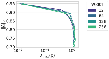
Figure 7: Norm of the residual and top eigenvalue of the GN matrix, where the vector field shows the evolution of these quantities during training for a fixed learning rate. Left: $\mu$P- note that all curves have a sharpening phase, after which the residual continues to decrease. Right: NTP - Increasing the width reduces the sharpening, since it approaches the infinite width limit where the NTK matrix becomes asymptotically constant.

We now perform experiments to test whether $\mathcal{G}$ dominates the residual for cross-entropy loss, in order to support our claim on the connection between feature learning and optimization. We plot the evolution of the largest eigenvalue of the GN matrix and the residual norm through time in Figure 7 for $\mu$P and NTP. The largest eigenvalue of this matrix is computed using a power iteration algorithm based on the implementation provided in Osawa et al. (2023). Note that while for $\mu$P we observe a large amount of progressive sharpening during training, for NTP the sharpness becomes asymptotically constant. The architecture used for the plot is a convolutional neural network as described in B, trained on CIFAR-10 for $10$ epochs using cross-entropy loss. These experiments confirm the results obtained for MSE loss in the main text (Fig. 5).

Appendix E Other Results

E.1 Late-time dynamics

It was noted in Cohen et al. (2021) (Appendix C) that with cross-entropy loss (adopted here), the sharpness decreases towards the end of training. Here in Fig. 8, we show that while the dynamics are remarkably consistent during the first part of training, they diverge during the phase transition in which the sharpness begins to drop, with wider models starting to exhibit the sharpness drop earlier. Hence, this transition point is highly width-dependent, and it coincides with a slight shift in the optimal learning rate. This late phase happens when the classifier maximizes the margin between classes Cohen et al. (2021), and can be largely prevented by using data augmentation techniques, as we exemplify in Sec. E.2.

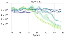
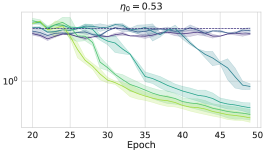
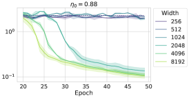
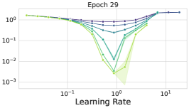
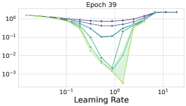
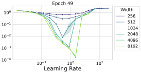
Figure 8: Late-time dynamics. We study the same setting as in Fig. 4 (for $\mu$P), under longer training time. Notice how when training longer, the sharpness decreases once the model gets closer to convergence. In this phase, there is a shift of the optimal learning rate, as the bottom row shows.

E.2 The effect of Batch Size and Data Augmentation

Batch Size

We test what happens to the sharpness and optimal learning rate when the batch size is increased. The sharpness is well-known to increase with the batch size, as it is shown also in Cohen et al. (2021) and Jastrzkebski et al. (2018). Here we add that under $\mu$P, the batch size we tested ($128$, $256$, $512$) do not influence significantly the width-independence phenomenon of the sharpness, as we summarize in Fig. 9. We observe good learning rate transfer across all the tested batch sizes. We also observe that the optimal learning rate increases with the batch sizes by roughly a factor of $2$.

Data Augmentation

We repeating the same experiment, varying the batch size, but this data we turn on data augmentation using standard transformations (random crops, horizontal flips, $10$-degrees rotations). The results are in Fig. 10 (to compare with Fig. 9). Notice how data augmentation has a stabilizing effect on the sharpness, delaying the late phase of training where the sharpness drops, as analyzed in Sec. E.1 Cohen et al. (2021), Kalra et al. (2023). Thus, under regularization techniques such as data augmentation, we should expect better hyperparameter transfer.

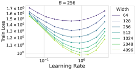
Figure 9: Batch size ablation. The red dashed line indicates the sharpness of $4/\eta_{0}$, only shown for the largest learning rate where the sharpness rises above the EoS threshold. Parameters: dataset: CIFAR-10, with data augmentation, epochs $=50$. The learning rate shown above are: (0.11, 0.32, 0.88, 2.45)

E.3 Large-Scale experiments

We provide empirical validation of our findings and show that in realistic architectures, such as Transformers (ViTs, GPT-2) and ResNets, we achieve width (or depth, respectively) independent sharpness. More concretely, we obtain learning rate transfer and width independent sharpness in Figures 11, 15 when training ResNets on TinyImagenet and Imagenet, as well as depth independent sharpness in Figures 12,  13,  14 for ResNets, ViTs and GPT-2. These results empirically demonstrate that our findings extend to different modalities and architectures.

Additionally, we perform ablations on the batch size in Figure 10 and show that smaller batch sizes lead to less sharpening than batch sizes, and thus in certain cases not reaching EoS, correlating our findings to those of Cohen et al. (2021).

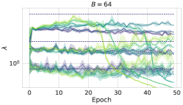
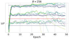
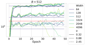
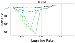
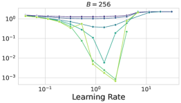
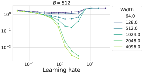
Figure 10: Batch size ablation. The red dashed line indicates the sharpness of $4/\eta_{0}$, only shown for the largest learning rate where the sharpness rises above the EoS threshold. Parameters: dataset: CIFAR-10, without data augmentation, epochs $=50$. The learning rate shown above are: (0.11, 0.32, 0.88, 2.45)

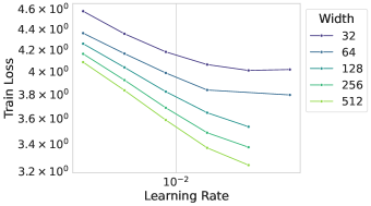
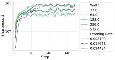
Figure 11: Residual convolutional networks (ResNets) trained on Tiny-ImageNet with stochastic gradient descent. Left figure shows the learning rate transfers across width in ResNets parameterized with $\mu$P. Right figure shows that for a fixed learning rate, the sharpness becomes width independent during training. Parameters: batch size $64$, epochs $10$.

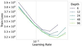
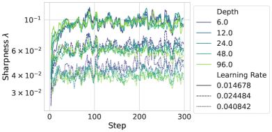
Figure 12: Residual convolutional networks trained on Tiny-ImageNet with stochastic gradient descent. Left figure shows the learning rate transfers across depth in ResNets parameterized with Depth$-\mu$P. Right figure shows that for a fixed learning rate, the sharpness becomes depth independent during training. Parameters: batch size $64$, epochs $10$.

References

- Ahn et al. (2022) K. Ahn, J. Zhang, and S. Sra. Understanding the unstable convergence of gradient descent. In International Conference on Machine Learning, pages 247–257. PMLR, 2022.
- Arora et al. (2019) S. Arora, S. S. Du, W. Hu, Z. Li, R. R. Salakhutdinov, and R. Wang. On exact computation with an infinitely wide neural net. Advances in neural information processing systems, 32, 2019.
- Arora et al. (2022) S. Arora, Z. Li, and A. Panigrahi. Understanding gradient descent on the edge of stability in deep learning. In International Conference on Machine Learning, pages 948–1024. PMLR, 2022.
- Bergstra and Bengio (2012) J. Bergstra and Y. Bengio. Random search for hyper-parameter optimization. Journal of machine learning research, 13(2), 2012.
- Bordelon and Pehlevan (2022) B. Bordelon and C. Pehlevan. Self-consistent dynamical field theory of kernel evolution in wide neural networks. Advances in Neural Information Processing Systems, 35:32240–32256, 2022.
- Bordelon and Pehlevan (2023) B. Bordelon and C. Pehlevan. Dynamics of finite width kernel and prediction fluctuations in mean field neural networks. arXiv preprint arXiv:2304.03408, 2023.
- Bordelon et al. (2023) B. Bordelon, L. Noci, M. B. Li, B. Hanin, and C. Pehlevan. Depthwise hyperparameter transfer in residual networks: Dynamics and scaling limit. arXiv preprint arXiv:2309.16620, 2023.
- Chizat and Bach (2018) L. Chizat and F. Bach. On the global convergence of gradient descent for over-parameterized models using optimal transport. Advances in neural information processing systems, 31, 2018.
- Chizat and Bach (2020) L. Chizat and F. Bach. Implicit bias of gradient descent for wide two-layer neural networks trained with the logistic loss. In Conference on Learning Theory, pages 1305–1338. PMLR, 2020.
- Chizat and Netrapalli (2023) L. Chizat and P. Netrapalli. Steering deep feature learning with backward aligned feature updates. arXiv preprint arXiv:2311.18718, 2023.
- Chizat et al. (2019) L. Chizat, E. Oyallon, and F. Bach. On lazy training in differentiable programming. Advances in neural information processing systems, 32, 2019.
- Claesen and Moor (2015) M. Claesen and B. D. Moor. Hyperparameter search in machine learning, 2015.
- Cohen et al. (2021) J. M. Cohen, S. Kaur, Y. Li, J. Z. Kolter, and A. Talwalkar. Gradient descent on neural networks typically occurs at the edge of stability. arXiv preprint arXiv:2103.00065, 2021.
- Cohen et al. (2022) J. M. Cohen, B. Ghorbani, S. Krishnan, N. Agarwal, S. Medapati, M. Badura, D. Suo, D. Cardoze, Z. Nado, G. E. Dahl, et al. Adaptive gradient methods at the edge of stability. arXiv preprint arXiv:2207.14484, 2022.
- Damian et al. (2022) A. Damian, E. Nichani, and J. D. Lee. Self-stabilization: The implicit bias of gradient descent at the edge of stability. arXiv preprint arXiv:2209.15594, 2022.
- Dosovitskiy et al. (2020) A. Dosovitskiy, L. Beyer, A. Kolesnikov, D. Weissenborn, X. Zhai, T. Unterthiner, M. Dehghani, M. Minderer, G. Heigold, S. Gelly, et al. An image is worth 16x16 words: Transformers for image recognition at scale. arXiv preprint arXiv:2010.11929, 2020.
- Franceschi et al. (2017) L. Franceschi, M. Donini, P. Frasconi, and M. Pontil. Forward and reverse gradient-based hyperparameter optimization. In International Conference on Machine Learning, pages 1165–1173. PMLR, 2017.
- Garriga-Alonso et al. (2018) A. Garriga-Alonso, C. E. Rasmussen, and L. Aitchison. Deep convolutional networks as shallow gaussian processes. arXiv preprint arXiv:1808.05587, 2018.
- Garrigos and Gower (2023) G. Garrigos and R. M. Gower. Handbook of convergence theorems for (stochastic) gradient methods. arXiv preprint arXiv:2301.11235, 2023.
- Goodfellow et al. (2016) I. Goodfellow, Y. Bengio, and A. Courville. Deep Learning. MIT Press, 2016. http://www.deeplearningbook.org.
- Gower et al. (2019) R. M. Gower, N. Loizou, X. Qian, A. Sailanbayev, E. Shulgin, and P. Richtárik. Sgd: General analysis and improved rates. In International conference on machine learning, pages 5200–5209. PMLR, 2019.
- Hanin and Nica (2019) B. Hanin and M. Nica. Finite depth and width corrections to the neural tangent kernel. arXiv preprint arXiv:1909.05989, 2019.
- Hanin and Nica (2020) B. Hanin and M. Nica. Products of many large random matrices and gradients in deep neural networks. Communications in Mathematical Physics, 376(1):287–322, 2020.
- Hayou (2022) S. Hayou. On the infinite-depth limit of finite-width neural networks. arXiv preprint arXiv:2210.00688, 2022.
- Hayou and Yang (2023) S. Hayou and G. Yang. Width and depth limits commute in residual networks. arXiv preprint arXiv:2302.00453, 2023.
- Hayou et al. (2021) S. Hayou, E. Clerico, B. He, G. Deligiannidis, A. Doucet, and J. Rousseau. Stable resnet. In International Conference on Artificial Intelligence and Statistics, pages 1324–1332. PMLR, 2021.
- He et al. (2015) K. He, X. Zhang, S. Ren, and J. Sun. Delving deep into rectifiers: Surpassing human-level performance on imagenet classification. In Proceedings of the IEEE international conference on computer vision, pages 1026–1034, 2015.
- Horváth et al. (2021) S. Horváth, A. Klein, P. Richtárik, and C. Archambeau. Hyperparameter transfer learning with adaptive complexity. In International Conference on Artificial Intelligence and Statistics, pages 1378–1386. PMLR, 2021.
- Hron et al. (2020) J. Hron, Y. Bahri, J. Sohl-Dickstein, and R. Novak. Infinite attention: Nngp and ntk for deep attention networks. In International Conference on Machine Learning, pages 4376–4386. PMLR, 2020.
- Iyer et al. (2023) G. Iyer, B. Hanin, and D. Rolnick. Maximal initial learning rates in deep relu networks. In International Conference on Machine Learning, pages 14500–14530. PMLR, 2023.
- Jacot et al. (2018) A. Jacot, F. Gabriel, and C. Hongler. Neural tangent kernel: Convergence and generalization in neural networks. Advances in neural information processing systems, 31, 2018.
- Jamieson and Talwalkar (2016) K. Jamieson and A. Talwalkar. Non-stochastic best arm identification and hyperparameter optimization. In Artificial intelligence and statistics, pages 240–248. PMLR, 2016.
- Jastrzebski et al. (2020) S. Jastrzebski, M. Szymczak, S. Fort, D. Arpit, J. Tabor, K. Cho, and K. Geras. The break-even point on optimization trajectories of deep neural networks. arXiv preprint arXiv:2002.09572, 2020.
- Jastrzkebski et al. (2018) S. Jastrzkebski, Z. Kenton, N. Ballas, A. Fischer, Y. Bengio, and A. Storkey. On the relation between the sharpest directions of dnn loss and the sgd step length. arXiv preprint arXiv:1807.05031, 2018.
- Jelassi et al. (2023) S. Jelassi, B. Hanin, Z. Ji, S. J. Reddi, S. Bhojanapalli, and S. Kumar. Depth dependence of mup learning rates in relu mlps. arXiv preprint arXiv:2305.07810, 2023.
- Kalra and Barkeshli (2023) D. S. Kalra and M. Barkeshli. Phase diagram of early training dynamics in deep neural networks: effect of the learning rate, depth, and width. In Thirty-seventh Conference on Neural Information Processing Systems, 2023.
- Kalra et al. (2023) D. S. Kalra, T. He, and M. Barkeshli. Universal sharpness dynamics in neural network training: Fixed point analysis, edge of stability, and route to chaos. arXiv preprint arXiv:2311.02076, 2023.
- Kingma and Ba (2014) D. P. Kingma and J. Ba. Adam: A method for stochastic optimization. arXiv preprint arXiv:1412.6980, 2014.
- LeCun (2002) e. a. LeCun, Yann. Efficient backprop. Neural networks: Tricks of the trade. Berlin, Heidelberg: Springer Berlin Heidelberg, 2002.
- LeCun et al. (2002) Y. LeCun, L. Bottou, G. B. Orr, and K.-R. Müller. Efficient backprop. In Neural networks: Tricks of the trade, pages 9–50. Springer, 2002.
- Lee et al. (2017) J. Lee, Y. Bahri, R. Novak, S. S. Schoenholz, J. Pennington, and J. Sohl-Dickstein. Deep neural networks as gaussian processes. arXiv preprint arXiv:1711.00165, 2017.
- Lee et al. (2019) J. Lee, L. Xiao, S. Schoenholz, Y. Bahri, R. Novak, J. Sohl-Dickstein, and J. Pennington. Wide neural networks of any depth evolve as linear models under gradient descent. Advances in neural information processing systems, 32, 2019.
- Lewkowycz et al. (2020) A. Lewkowycz, Y. Bahri, E. Dyer, J. Sohl-Dickstein, and G. Gur-Ari. The large learning rate phase of deep learning: the catapult mechanism. arXiv preprint arXiv:2003.02218, 2020.
- Li et al. (2018) L. Li, K. Jamieson, G. DeSalvo, A. Rostamizadeh, and A. Talwalkar. Hyperband: A novel bandit-based approach to hyperparameter optimization. Journal of Machine Learning Research, 18(185):1–52, 2018.
- Li et al. (2021) M. Li, M. Nica, and D. Roy. The future is log-gaussian: Resnets and their infinite-depth-and-width limit at initialization. Advances in Neural Information Processing Systems, 34:7852–7864, 2021.
- Li et al. (2022) M. Li, M. Nica, and D. Roy. The neural covariance sde: Shaped infinite depth-and-width networks at initialization. Advances in Neural Information Processing Systems, 35:10795–10808, 2022.
- Li and Nica (2023) M. B. Li and M. Nica. Differential equation scaling limits of shaped and unshaped neural networks. arXiv preprint arXiv:2310.12079, 2023.
- Li et al. (2019) Y. Li, C. Wei, and T. Ma. Towards explaining the regularization effect of initial large learning rate in training neural networks. Advances in Neural Information Processing Systems, 32, 2019.
- Maclaurin et al. (2015) D. Maclaurin, D. Duvenaud, and R. Adams. Gradient-based hyperparameter optimization through reversible learning. In International conference on machine learning, pages 2113–2122. PMLR, 2015.
- Martens (2016) J. Martens. Second-order optimization for neural networks. University of Toronto (Canada), 2016.
- Martens (2020) J. Martens. New insights and perspectives on the natural gradient method. The Journal of Machine Learning Research, 21(1):5776–5851, 2020.
- Mei et al. (2019) S. Mei, T. Misiakiewicz, and A. Montanari. Mean-field theory of two-layers neural networks: dimension-free bounds and kernel limit. In Conference on Learning Theory, pages 2388–2464. PMLR, 2019.
- Neal (1995) R. M. Neal. Bayesian Learning for Neural Networks. PhD thesis, University of Toronto, 1995.
- Nesterov (2013) Y. Nesterov. Introductory lectures on convex optimization: A basic course, volume 87. Springer Science & Business Media, 2013.
- Noci et al. (2021) L. Noci, G. Bachmann, K. Roth, S. Nowozin, and T. Hofmann. Precise characterization of the prior predictive distribution of deep relu networks. Advances in Neural Information Processing Systems, 34:20851–20862, 2021.
- Noci et al. (2022) L. Noci, S. Anagnostidis, L. Biggio, A. Orvieto, S. P. Singh, and A. Lucchi. Signal propagation in transformers: Theoretical perspectives and the role of rank collapse. Advances in Neural Information Processing Systems, 35:27198–27211, 2022.
- Noci et al. (2023) L. Noci, C. Li, M. B. Li, B. He, T. Hofmann, C. Maddison, and D. M. Roy. The shaped transformer: Attention models in the infinite depth-and-width limit. arXiv preprint arXiv:2306.17759, 2023.
- Orvieto et al. (2021) A. Orvieto, J. Kohler, D. Pavllo, T. Hofmann, and A. Lucchi. Vanishing curvature and the power of adaptive methods in randomly initialized deep networks. arXiv preprint arXiv:2106.03763, 2021.
- Osawa et al. (2023) K. Osawa, S. Ishikawa, R. Yokota, S. Li, and T. Hoefler. Asdl: A unified interface for gradient preconditioning in pytorch. arXiv preprint arXiv:2305.04684, 2023.
- Ott (2002) E. Ott. Chaos in dynamical systems. Cambridge university press, 2002.
- Perrone et al. (2018) V. Perrone, R. Jenatton, M. W. Seeger, and C. Archambeau. Scalable hyperparameter transfer learning. Advances in neural information processing systems, 31, 2018.
- Radford et al. (2019) A. Radford, J. Wu, R. Child, D. Luan, D. Amodei, I. Sutskever, et al. Language models are unsupervised multitask learners. OpenAI blog, 1(8):9, 2019.
- Sagun et al. (2016) L. Sagun, L. Bottou, and Y. LeCun. Eigenvalues of the hessian in deep learning: Singularity and beyond. arXiv preprint arXiv:1611.07476, 2016.
- Shaban et al. (2019) A. Shaban, C.-A. Cheng, N. Hatch, and B. Boots. Truncated back-propagation for bilevel optimization. In The 22nd International Conference on Artificial Intelligence and Statistics, pages 1723–1732. PMLR, 2019.
- Singh et al. (2021) S. P. Singh, G. Bachmann, and T. Hofmann. Analytic insights into structure and rank of neural network hessian maps. Advances in Neural Information Processing Systems, 34:23914–23927, 2021.
- Smith and Topin (2019) L. N. Smith and N. Topin. Super-convergence: Very fast training of neural networks using large learning rates. In Artificial intelligence and machine learning for multi-domain operations applications, volume 11006, pages 369–386. SPIE, 2019.
- Snoek et al. (2012) J. Snoek, H. Larochelle, and R. P. Adams. Practical bayesian optimization of machine learning algorithms. Advances in neural information processing systems, 25, 2012.
- Snoek et al. (2015) J. Snoek, O. Rippel, K. Swersky, R. Kiros, N. Satish, N. Sundaram, M. Patwary, M. Prabhat, and R. Adams. Scalable bayesian optimization using deep neural networks. In International conference on machine learning, pages 2171–2180. PMLR, 2015.
- Song and Yun (2023) M. Song and C. Yun. Trajectory alignment: understanding the edge of stability phenomenon via bifurcation theory. arXiv preprint arXiv:2307.04204, 2023.
- Stoll et al. (2020) D. Stoll, J. K. Franke, D. Wagner, S. Selg, and F. Hutter. Hyperparameter transfer across developer adjustments. arXiv preprint arXiv:2010.13117, 2020.
- Vyas et al. (2023) N. Vyas, A. Atanasov, B. Bordelon, D. Morwani, S. Sainathan, and C. Pehlevan. Feature-learning networks are consistent across widths at realistic scales. arXiv preprint arXiv:2305.18411, 2023.
- Yaida (2020) S. Yaida. Non-gaussian processes and neural networks at finite widths. In Mathematical and Scientific Machine Learning, pages 165–192. PMLR, 2020.
- Yaida (2022) S. Yaida. Meta-principled family of hyperparameter scaling strategies. arXiv preprint arXiv:2210.04909, 2022.
- Yang (2020) G. Yang. Tensor programs ii: Neural tangent kernel for any architecture. arXiv preprint arXiv:2006.14548, 2020.
- Yang and Hu (2021) G. Yang and E. J. Hu. Tensor programs iv: Feature learning in infinite-width neural networks. In International Conference on Machine Learning, pages 11727–11737. PMLR, 2021.
- Yang and Littwin (2023) G. Yang and E. Littwin. Tensor programs ivb: Adaptive optimization in the infinite-width limit. arXiv preprint arXiv:2308.01814, 2023.
- Yang et al. (2022) G. Yang, E. J. Hu, I. Babuschkin, S. Sidor, X. Liu, D. Farhi, N. Ryder, J. Pachocki, W. Chen, and J. Gao. Tensor programs v: Tuning large neural networks via zero-shot hyperparameter transfer. arXiv preprint arXiv:2203.03466, 2022.
- Yang et al. (2023) G. Yang, D. Yu, C. Zhu, and S. Hayou. Tensor programs vi: Feature learning in infinite-depth neural networks. arXiv preprint arXiv:2310.02244, 2023.
- Yao et al. (2020) Z. Yao, A. Gholami, K. Keutzer, and M. W. Mahoney. Pyhessian: Neural networks through the lens of the hessian. In 2020 IEEE international conference on big data (Big data), pages 581–590. IEEE, 2020.
- Yogatama and Mann (2014) D. Yogatama and G. Mann. Efficient transfer learning method for automatic hyperparameter tuning. In Artificial intelligence and statistics, pages 1077–1085. PMLR, 2014.
- Zavatone-Veth et al. (2021) J. Zavatone-Veth, A. Canatar, B. Ruben, and C. Pehlevan. Asymptotics of representation learning in finite bayesian neural networks. Advances in neural information processing systems, 34:24765–24777, 2021.
- Zhao et al. (2023) W. X. Zhao, K. Zhou, J. Li, T. Tang, X. Wang, Y. Hou, Y. Min, B. Zhang, J. Zhang, Z. Dong, Y. Du, C. Yang, Y. Chen, Z. Chen, J. Jiang, R. Ren, Y. Li, X. Tang, Z. Liu, P. Liu, J.-Y. Nie, and J.-R. Wen. A survey of large language models. arXiv preprint arXiv:2303.18223, 2023. URL http://arxiv.org/abs/2303.18223.
- Zhu et al. (2022) X. Zhu, Z. Wang, X. Wang, M. Zhou, and R. Ge. Understanding edge-of-stability training dynamics with a minimalist example. arXiv preprint arXiv:2210.03294, 2022.