Abstract.

Among the various models designed for dependent count data, integer-valued autoregressive (INAR) processes enjoy great popularity. Typically, statistical inference for INAR models uses asymptotic theory that relies on rather stringent (parametric) assumptions on the innovations such as Poisson or negative binomial distributions. In this paper, we present a novel semi-parametric goodness-of-fit test tailored for the INAR model class. Relying on the INAR-specific shape of the joint probability generating function, our approach allows for model validation of INAR models without specifying the (family of the) innovation distribution. We derive the limiting null distribution of our proposed test statistic, prove consistency under fixed alternatives and discuss its asymptotic behavior under local alternatives. By manifold Monte Carlo simulations, we illustrate the overall good performance of our testing procedure in terms of power and size properties. In particular, it turns out that the power can be considerably improved by using higher-order test statistics. We conclude the article with the application on three real-world economic data sets.

Keywords: Bootstrap, count time series, goodness-of-fit, INAR models, probability generating function, semi-parametric estimation

1. Introduction

Integer-valued autoregressive (INAR) models represent a powerful model class for modeling count time series. They offer a flexible and versatile approach for dealing with autoregressive (AR) time series of non-negative integer values and are the natural analog of the well-known AR model for continuous-valued time series. [11] introduce the INAR model of order $p$ to follow the recursion

$$X_{t}=\alpha_{1}\circ X_{t-1}+\ldots+\alpha_{p}\circ X_{t-p}+\varepsilon_{t},\quad t\in\mathbb{Z}=\{\ldots,-1,0,1,\ldots\},$$ (1.1)

where $\varepsilon_{t}\overset{\text{i.i.d.}}{\sim}G$, that is, the innovations $(\varepsilon_{t},t\in\mathbb{Z})$ are independent and identically distributed and follow a discrete distribution $G$ with range $\mathbb{N}_{0}=\{0,1,2,\ldots\}$ and probability mass function (pmf) $(G(k),\,k\in\mathbb{N}_{0})$. The vector of model coefficients $\boldsymbol{\alpha}=(\alpha_{1},\ldots,\alpha_{p})\in(0,1)^{p}$ fulfills $\sum_{j=1}^{p}\alpha_{j}<1$. To ensure the integer-valued modeling of the time series, the model uses the binomial thinning operator “$\circ$” introduced by [32] as

$$\alpha_{j}\circ X_{t-j}=\sum\limits_{i=1}^{X_{t-j}}Z_{i}^{(t,j)},$$ (1.2)

with $\left(Z_{i}^{(t,j)},i\in\mathbb{N},t\in\mathbb{Z}\right)$, $j\in\{1,\ldots,p\}$ being mutually independent Bernoulli-distributed random variables $Z_{i}^{(t,j)}\sim\text{Bin}(1,\alpha_{j})$ independent of ($\varepsilon_{t},\,t\in\mathbb{Z}$). Hence, the thinning operations are independent over time and independent of ($\varepsilon_{t},\,t\in\mathbb{Z}$). Additionally, the thinning operation at time $t$ and $\varepsilon_{t}$ are both independent of $X_{s},\,s<t$. These comprehensive independence assumptions are characteristic for the INAR$(p)$ model formulation of [11] and they differ from the one of [2]. But as only the INAR$(p)$ model of [11] leads to the traditional Yule–Walker equations for the autocorrelation function (ACF), this model is usually preferred in practice and we focus on this model specification for the remainder of this paper. However, for $p=1$, both versions of INAR($p$) models simplify to the INAR(1) model first introduced by [26] and [1].

The aforementioned flexibility of INAR models gets lost if one imposes a (parametric) family of distributions for the innovations, which, however, mostly happens in the literature because it simplifies considerably the estimation and the inference for these models. Initially, [1] suggested a Poisson distribution for the innovations, which can be considered as the natural analog of the normal distribution in the continuous case. However, a Poisson distribution may be too restrictive in applications as it only allows for equidispersion. In the following years, INAR models with several alternative innovation distributions have been considered. For instance, [30] deal with negative binomial innovations, [21] with geometric innovations, and [20] with a zero-inflated Poisson innovation distribution. But regardless of which innovation distribution we choose, we will always face restrictions and lose some of the flexibility of the INAR($p$) model in (1.1). That is why we should not test for restrictive (parametric) null hypotheses $H_{0}^{\text{para}}$ with pre-defined innovation distribution, where

$$H_{0}^{\text{para}}:(X_{t},\,t\in\mathbb{Z})\;\text{is INAR($p$) with $G=G_{\lambda}$ for some $\lambda\in\Lambda$}$$ (1.3)

for some parametric family of innovation distributions $\{G_{\lambda},\,\lambda\in\Lambda\}$ with $\Lambda\subset\mathbb{R}^{d}$ for some (finite) $d$ as it is usually considered in the literature, see e.g. [27], [18], [31], [3], and [4]. Such parametric assumptions considerably facilitate the estimation and allow for relatively simple testing strategies, but they also make the tests prone to possible model misspecification. Instead, we want to test the (semi-parametric) null hypothesis $H_{0}^{\text{semi}}$ that the data at hand follow an INAR($p$) model as in (1.1) with unspecified innovation distribution, i.e.

$$H_{0}^{\text{semi}}:(X_{t},\,t\in\mathbb{Z})\;\text{is INAR($p$).}$$ (1.4)

In practice, irrespective of the concrete underlying innovation distribution, it is very helpful to know whether an INAR($p$) process (1.1) is suitable to adequately capture the dependence structure of the count time series. In this case, a semi-parametric estimation approach can be used. The general relevance of semi-parametric approaches for $\mathbb{Z}$-valued time series was recently demonstrated by [25], who consider a similar model setup. In a more general time series setup, [5] introduce the semi-parametric pseudo-variance quasi-maximum-likelihood estimation which is based on a Gaussian quasi-likelihood function relying on the specification of the pseudo-variance. The latter transfer naturally to time series of bounded counts, which are not considered here. Instead, we use the semi-parametric estimator of [10], which does not impose any parametric assumption on the innovation distribution and estimates $G$ non-parametrically. Hence, even without imposing a parametric assumption on the innovation distribution, such (semi-parametric) INAR processes are generally attractive in applications as they are very flexible and still easily interpretable due to their autoregressive nature.

The paper is organized as follows. We introduce a test statistic for the null hypothesis defined in (1.4), derive its null limiting distribution and prove its asymptotic behavior under fixed and local alternatives in Section 2. As the limiting null distribution is cumbersome to estimate, we introduce an appropriate bootstrap procedure in Section 3 to get critical values. Corresponding simulation results are provided in Section 4. Three applications on real-world data sets follow in Section 5. The paper concludes with Section 6, where we summarize the results and give an outlook on possible future research questions. All proofs are deferred to an appendix.

2. Semi-Parametric Goodness-of-Fit Test for INAR Models

Suppose we observe a sample $X_{1},\ldots,X_{n}$ of time-series count data and we want to construct a test statistic for the null hypothesis $H_{0}^{\text{semi}}$ in (1.4). While [27] exclusively consider parametric null hypotheses $H_{0}^{\text{para}}$ of the form (1.3) without providing asymptotic theory, we adopt their idea of constructing a suitable $L_{2}$-type test statistic based on two estimators of the (joint) probability generating function (pgf). The first pgf estimator shall be consistent in general, and the second one only under the null $H_{0}^{\text{semi}}$. In [27], the pgf estimation under their (parametric) null $H_{0}^{\text{para}}$ facilitates a lot due to their parametric assumption on the innovations, which results in closed form expressions for the pgf, depending on a finite number of estimated parameters determining the innovation distribution. In what follows, by contrast, we deal with more general expressions under the semi-parametric setup in (1.1).

2.1. Joint probability generating function of INAR models

As we want to test for INAR-type dependence structure of order $p$, we consider the joint pgf of $p+1$ consecutive random variables $X_{t},\ldots,X_{t-p}$, which uniquely determines the full dependence structure of a Markov process of order $p$. Then, for $u_{0},\ldots,u_{p}\in[0,1]$, the joint pgf of $X_{t},\ldots,X_{t-p}$ is defined as

$$g_{p}(u_{0},\ldots,u_{p}):=g_{X_{t},\ldots,X_{t-p}}(u_{0},\ldots,u_{p}):=E\big{(}u_{0}^{X_{t}}\cdots u_{p}^{X_{t-p}}\big{)}.$$ (2.1)

For the construction of a suitable pgf-based goodness-of-fit test statistic, we exploit the INAR dependence structure of $X_{t},\ldots,X_{t-p}$ and derive an explicit representation of the joint pgf $g_{p}$ for INAR($p$) models.

Lemma 2.1 (Joint pgf of INAR($p$) processes).

For $X_{t},\ldots,X_{t-p}$ following an INAR($p$) process (1.1), the pgf $g_{p}$ defined in (2.1) can be represented by

$$g_{p}(u_{0}\ldots,u_{p})=g_{\varepsilon}(u_{0})\cdot E\left(\prod_{j=1}^{p}\Big{\{}u_{j}\big{(}1+\alpha_{j}(u_{0}-1)\big{)}\Big{\}}^{X_{t-j}}\right),$$ (2.2)

where $g_{\varepsilon}(u_{0})=\sum_{k=0}^{\infty}P(\varepsilon_{t}=k)\,u_{0}^{k}=\sum_{k=0}^{\infty}G(k)\,u_{0}^{k}$.

The proof is contained in Subsection A.1 in the Appendix. Taking a closer look at (2.2), we see that the pgf $g_{p}$ can be represented as a product of two factors. While the first factor exclusively depends on the pmf of the innovation distribution, $(G(k),\,k\in\mathbb{N}_{0})$, the second factor is the joint pgf of (only) $p$ consecutive random variables $X_{t-1},\ldots,X_{t-p}$, whose arguments $u_{j}(1+\alpha_{j}(u_{0}-1))$, $j=1,\ldots,p$ also depend on the autoregressive model coefficients $\alpha_{1},\ldots,\alpha_{p}$. Note that the representation (2.2) does not require any further (parametric) assumptions on $G$.

2.2. Goodness-of-fit test statistic

When we renounce all parametric assumptions on the innovation distribution, the main challenge is the estimation of the INAR model, determined by the model coefficients $\alpha_{1},\ldots,\alpha_{p}$ and the innovation distribution $G$. We cannot resort to (parametric) estimation methods such as moment or (conditional) maximum-likelihood estimation (see e.g. [34]) that are usually employed to consistently estimate the (low-dimensional) parameter vector determining the innovation distribution. Instead, we use the semi-parametric estimator introduced in [10], which maintains the parametric binomial thinning, while simultaneously enabling the non-parametric estimation of the innovation distribution. For a small-sample refinement of this semi-parametric estimator using penalization techniques, we refer to [12].

The estimation procedure proposed by [10] allows for joint estimation of the INAR coefficients and the pmf of the innovation distribution, $(G(k),\,k\in\mathbb{N}_{0})$. Given $X_{1},\ldots,X_{n}$, their semi-parametric maximum-likelihood estimator

$$(\boldsymbol{\widehat{\alpha}}_{\text{sp}},\widehat{G}_{\text{sp}})=(\widehat{\alpha}_{\text{sp},1},\ldots,\widehat{\alpha}_{\text{sp},p},\widehat{G}_{\text{sp}}(0),\widehat{G}_{\text{sp}}(1),\ldots),$$ (2.3)

which they prove to be consistent and efficient, is defined to maximize the conditional likelihood, i.e.

$$(\widehat{\boldsymbol{\alpha}}_{\text{sp}},\widehat{G}_{\text{sp}})\in\underset{(\boldsymbol{\alpha},G)\in[0,1]^{p}\times\widetilde{\mathcal{G}}}{\text{arg max}}\left(\prod\limits_{t=p+1}^{n}P^{\boldsymbol{\alpha},G}_{(X_{t-1},\ldots,X_{t-p}),X_{t}}\right),$$ (2.4)

where $\widetilde{\mathcal{G}}$ contains all probability measures on $\mathbb{N}_{0}$ and $P^{\boldsymbol{\alpha},G}_{(X_{t-1},\ldots,X_{t-p}),X_{t}}$ denotes the transition probabilities

$$P^{\boldsymbol{\alpha},G}_{(x_{t-1},\ldots,x_{t-p}),x_{t}} =\mathbb{P}_{\boldsymbol{\alpha},G}\left(\sum\limits_{j=1}^{p}\alpha_{i}\circ X_{t-j}+\varepsilon_{t}=x_{t}\mid X_{t-1}=x_{t-1},\ldots,X_{t-p}=x_{t-p}\right)$$

$$=(\text{Bin}(x_{t-1},\alpha_{1})\ast\ldots\ast\text{Bin}(x_{t-p},\alpha_{p})\ast G)\{x_{t}\}.$$

Here, $\mathbb{P}_{\boldsymbol{\alpha},G}$ denotes the underlying probability measure induced by an INAR($p$) process with coefficients $\boldsymbol{\alpha}$ and innovation distribution $G$, $\text{Bin}(x_{t-j},\alpha_{j})$ is the binomial distribution with parameters $x_{t-j}$ and $\alpha_{j}$, $j=1,\ldots,p$ and “$\ast$” denotes the convolution of distributions. The estimator in (2.3) allows to estimate the pgf in (2.2) under the semi-parametric null $H_{0}^{\text{semi}}$ in (1.4) without using any parametric assumption on the innovation distribution. Naturally, we use the plug-in estimator

$$\widehat{g}_{p;H_{0}}(u_{0},\ldots,u_{p}) :=\widehat{g}_{\varepsilon}(u_{0})\cdot\frac{1}{n-p}\sum_{t=p+1}^{n}\prod_{j=1}^{p}\Big{\{}u_{j}\big{(}1+\widehat{\alpha}_{\text{sp},j}(u_{0}-1)\big{)}\Big{\}}^{X_{t-j}},$$ (2.5)

where

$$\widehat{g}_{\varepsilon}(u_{0}) :=\sum_{k=0}^{\infty}\widehat{P}(\varepsilon_{t}=k)\,u_{0}^{k}=\sum_{k=0}^{\infty}\widehat{G}_{\text{sp}}(k)\,u_{0}^{k}=\sum_{k=0}^{\max(X_{1},\ldots,X_{n})}\widehat{G}_{\text{sp}}(k)\,u_{0}^{k}$$ (2.6)

with the semi-parametric estimators $\widehat{\alpha}_{\text{sp},j},\,j\in\{1,\ldots,p\}$ and $(\widehat{G}_{\text{sp}}(k),\,k\in\mathbb{N}_{0})$ from (2.3). The last equality in (2.6) holds, because, for fixed $n\in\mathbb{N}$, we have $\widehat{G}_{\text{sp}}(k)=0\;\forall k>\max(X_{1},\ldots,X_{n})$; see [10] for details.

While the estimator $\widehat{g}_{p;H_{0}}(u_{0},\ldots,u_{p})$ explicitly makes use of the INAR structure, the following (non-parametric) estimator is consistent in general, that is, under the null and under the alternative:

$$\widehat{g}_{p}(u_{0},\ldots,u_{p}):=\frac{1}{n-p}\sum_{t=p+1}^{n}\prod_{j=0}^{p}u_{j}^{X_{t-j}}.$$ (2.7)

Hence, under the null $H_{0}^{\text{semi}}$ in (1.4) of an underlying INAR($p$) process, both $\widehat{g}_{p;H_{0}}(u_{0},\ldots,u_{p})$ and $\widehat{g}_{p}(u_{0},\ldots,u_{p})$ estimate the same quantity. This allows construct the $L_{2}$-type test statistic defined as

$$T_{n}=n\int_{0}^{1}\cdots\int_{0}^{1}\Big{(}\widehat{g}_{p;H_{0}}(u_{0},\ldots,u_{p})-\widehat{g}_{p}(u_{0},\ldots,u_{p})\Big{)}^{2}\,w(u_{0},\ldots,u_{p};a)\,du_{0}\cdots du_{p},$$ (2.8)

where $w(u_{0},\ldots,u_{p};a):=(a+1)^{p+1}\prod\limits_{j=0}^{p}u_{j}^{a}$ is a weighting function with weighting parameter $a\geq 0$. The weighting function is constructed to integrate to one such that $w$ becomes a probability density function (pdf) on $[0,1]^{p+1}$. Choosing $a=0$ corresponds to no weighting, whereas larger values for $a>0$ (common choices are $a=2$ and $a=5$) put more weight close to the right boundaries of the integration intervals $[0,1]$, see [16]. In what follows, we shall use a more precise notation of $T_{n}$ introduced in (2.8). Note that $T_{n}$ is naturally a function of $X_{1},\ldots,X_{n}$, but also that the definition of $T_{n}$ relies on (nuisance) parameter estimators $\widehat{\theta}_{\text{sp}}:=(\boldsymbol{\widehat{\alpha}}_{\text{sp}},\widehat{G}_{\text{sp}})$, which are also functions of $X_{1},\ldots,X_{n}$ themselves. This justifies the following notations:

$$T_{n}=T_{n}(X_{1},\ldots,X_{n})=T_{n}(\widehat{\theta}_{\text{sp}};X_{1},\ldots,X_{n})=T_{n}(\widehat{\theta}_{\text{sp}}).$$ (2.9)

The test statistic $T_{n}$ in (2.8) is of a similar structure as in [27]. However, by contrast to their parametric approach, we are using the semi-parametric estimator $\widehat{\theta}_{\text{sp}}=(\boldsymbol{\widehat{\alpha}}_{\text{sp}},\widehat{G}_{\text{sp}})$ from (2.3). We should reject the null hypothesis (1.4) for large values of (2.8).

Remark 2.2 (Higher-order test statistics).

For the construction of test statistics in the spirit of (2.8) to test for the null $H_{0}^{\text{semi}}$ in (1.4), we could also consider pgfs of higher order $s\geq p$, which may be beneficial to better detect Markov chain alternatives of higher order than $p$. That is, for any $s\geq p$, we can define the test statistic

$$T_{n}^{(s)}=n\int_{0}^{1}\cdots\int_{0}^{1}\Big{(}\widehat{g}_{s;H_{0}}(u_{0},\ldots,u_{s})-\widehat{g}_{s}(u_{0},\ldots,u_{s})\Big{)}^{2}\,w(u_{0},\ldots,u_{s};a)\,du_{0}\cdots du_{s},$$ (2.10)

where $\widehat{g}_{s}$ is defined as in (2.7) and

$$\widehat{g}_{s;H_{0}}(u_{0},\ldots,u_{s})=\widehat{g}_{\varepsilon}(u_{0})\cdot\frac{1}{n-s}\sum_{t=s+1}^{n}\prod_{j=1}^{s}\Big{\{}u_{j}\big{(}1+\widehat{\alpha}_{\text{sp},j}(u_{0}-1)\big{)}\Big{\}}^{X_{t-j}}$$

with $\widehat{\alpha}_{\text{sp},j}:=0$ for $j=p+1,\ldots,s$. Note that $T_{n}^{(p)}=T_{n}$ holds.

While the test statistic $T_{n}$ as proposed in (2.8) requires (numerical) integration, making use of (2.5) and (2.7), it can also be expressed without any integrals.

Lemma 2.3 (Calculation of $T_{n}$ without integrals).

The test statistic $T_{n}$ given by (2.8) can be equivalently written as

$$T_{n} =\frac{n}{(n-p)^{2}}(a+1)^{p+1}\left(\prod\limits_{j=1}^{p}\frac{1}{1+X_{t-j}+X_{s-j}+a}\right)\Bigg{[}\frac{1}{1+X_{t}+X_{s}+a}$$

$$+\sum\limits_{k_{1},k_{2}=0}^{\max(X_{1},\ldots,X_{n})}\widehat{G}_{\text{sp}}(k_{1})\widehat{G}_{\text{sp}}(k_{2})\sum\limits_{i_{1}=0}^{X_{t-1}+X_{s-1}}\sum\limits_{h_{1}=0}^{i_{1}}\ldots\sum\limits_{i_{p}=0}^{X_{t-p}+X_{s-p}}\sum\limits_{h_{p}=0}^{i_{p}}\frac{1}{1+k_{1}+k_{2}+a+\sum_{m=1}^{p}h_{m}}$$

$$\prod\limits_{j=1}^{p}\binom{X_{t-j}+X_{s-j}}{i_{j}}\widehat{\alpha}_{\text{sp},j}^{i_{j}}(-1)^{i_{j}-h_{j}}\binom{i_{j}}{h_{j}}-2\sum\limits_{k=0}^{\max(X_{1},\ldots,X_{n})}\widehat{G}_{\text{sp}}(k)$$

$$\sum\limits_{i_{1}=0}^{X_{t-1}+X_{s-1}}\sum\limits_{h_{1}=0}^{i_{1}}\ldots\sum\limits_{i_{p}=0}^{X_{t-p}+X_{s-p}}\sum\limits_{h_{p}=0}^{i_{p}}\frac{1}{1+k+X_{s}+a+\sum_{m=1}^{p}h_{m}}\prod\limits_{j=1}^{p}\binom{X_{t-j}}{i_{j}}\widehat{\alpha}_{\text{sp},j}^{i_{j}}(-1)^{i_{j}-h_{j}}\binom{i_{j}}{h_{j}}\Bigg{]}.$$

The proof is contained in Subsection A.2 in the Appendix.

2.3. Asymptotic theory

To derive the limiting distribution of our test statistic $T_{n}$, recall that, according to $\eqref{eq:tn_int_notation}$, we are actually confronted with $T_{n}(\widehat{\theta}_{\text{sp}})$. Before addressing this case in Section 2.3.2 below, let us consider first the somewhat simpler case of $T_{n}(\theta_{0})$ in Section 2.3.1, where the semi-parametric estimator $\widehat{\theta}_{\text{sp}}$ is replaced by some $\theta_{0}=(\boldsymbol{\alpha}_{0},G_{0})\in[0,1]^{p}\times\mathcal{\widetilde{G}}$.

2.3.1. Limiting distribution of $T_{n}(\theta_{0})$

Let us consider the test statistic $T_{n}(\theta_{0})=T_{n}(\theta_{0};X_{1},\ldots,X_{n})$ in more detail. It is defined similarly to $T_{n}=T_{n}(\widehat{\theta}_{\text{sp}})$ in (2.8), but with $\widehat{g}_{p;H_{0}}$ in (2.5) replaced by $g_{p;H_{0}}$, where

$$g_{p;H_{0}}(u_{0},\ldots,u_{p}) :=g_{0,\varepsilon}(u_{0})\cdot\frac{1}{n-p}\sum_{t=p+1}^{n}\prod_{j=1}^{p}\Big{\{}u_{j}\big{(}1+\alpha_{0,j}(u_{0}-1)\big{)}\Big{\}}^{X_{t-j}},$$

with $g_{0,\varepsilon}(u_{0}):=\sum_{k=0}^{\infty}G_{0}(k)\,u_{0}^{k}$. While the original test statistic $T_{n}(\widehat{\theta}_{\text{sp}})$ introduced in (2.8) allows to test for $H_{0}^{\text{semi}}$, that is, for the whole INAR($p$) model class, $T_{n}(\theta_{0})$ is useful to test for null hypotheses of the form

$$H_{0}^{\text{semi}}(\theta_{0}):(X_{t},\,t\in\mathbb{Z})\;\text{is INAR($p$) with $\theta=\theta_{0}$}$$ (2.11)

for $\theta_{0}=(\boldsymbol{\alpha}_{0},G_{0})$ with some pre-specified $\boldsymbol{\alpha}_{0}=(\alpha_{0,1},\ldots,\alpha_{0,p})$ and $G_{0}=(G_{0}(k),\,k\in\mathbb{N}_{0})$. Note that $H_{0}^{\text{semi}}(\theta_{0})\subset H_{0}^{\text{semi}}$ for all $\theta_{0}\in[0,1]^{p}\times\mathcal{\widetilde{G}}$.

The following proposition shows that, under the null $H_{0}^{\text{semi}}(\theta_{0})$, the test statistic $T_{n}(\theta_{0})$ can be represented as a degenerate V-statistic, which enables the derivation of its limiting distribution.

Proposition 2.4 ($T_{n}(\theta_{0})$ as a V-statistic).

Let $\theta_{0}\in[0,1]^{p}\times\mathcal{\widetilde{G}}$. Suppose the null hypothesis $H_{0}^{\text{semi}}(\theta_{0})$ in (2.11) holds, that is, $X_{1},\ldots,X_{n}$ follow an INAR($p$) process with coefficients $\boldsymbol{\alpha}_{0}=(\alpha_{0,1},\ldots,\alpha_{0,p})$ and innovation distribution $G_{0}=(G_{0}(k),\,k\in\mathbb{N}_{0})$. Then, the test statistic $T_{n}(\theta_{0})$ is a degenerate V-statistic. That is, $T_{n}(\theta_{0})$ can be represented as

$$T_{n}(\theta_{0})=\frac{n}{(n-p)^{2}}\sum\limits_{t=p+1}^{n}\sum\limits_{s=p+1}^{n}h(Y_{t},Y_{s};\theta_{0}),$$

where $Y_{t}=(X_{t},\ldots,X_{t-p})$, $Y_{s}=(X_{s},\ldots,X_{s-p})$, $\theta_{0}=(\boldsymbol{\alpha}_{0},G_{0})$ and $h:\mathbb{R}^{p+1}\times\mathbb{R}^{p+1}\rightarrow\mathbb{R}$ with

$$h(Y_{t},Y_{s};\theta_{0})= \int\limits_{0}^{1}\ldots\int\limits_{0}^{1}\left(g_{0,\varepsilon}(u_{0})\prod\limits_{j=1}^{p}(u_{j}(1+\alpha_{0,j}(u_{0}-1)))^{X_{t-j}}-\prod\limits_{j=0}^{p}u_{j}^{X_{t-j}}\right)$$ (2.12)

$$\times\left(g_{0,\varepsilon}(u_{0})\prod\limits_{j=1}^{p}(u_{j}(1+\alpha_{0,j}(u_{0}-1)))^{X_{s-j}}-\prod\limits_{j=0}^{p}u_{j}^{X_{s-j}}\right)w(u_{0},\ldots,u_{p};a)\,du_{0}\ldots du_{p}$$

the symmetric and continuous kernel and $E(h(y_{t},Y_{s};\theta_{0}))=0$ for all $y_{t}=(x_{t},\ldots,x_{t-p})\in\mathbb{R}^{p+1}$.

The proof is contained in Subsection A.3 in the Appendix. This finding allows to use the asymptotic results established for degenerate $V$-statistics by [24], which leads to the following theorem.

Theorem 2.5 (Limiting distribution of $T_{n}(\theta_{0})$ under $H_{0}^{\text{semi}}(\theta_{0})$).

Let $\theta_{0}\in[0,1]^{p}\times\mathcal{\widetilde{G}}$. Suppose the null hypothesis $H_{0}^{\text{semi}}(\theta_{0})$ in (2.11) holds, that is, $X_{1},\ldots,X_{n}$ follow an INAR($p$) process with coefficients $\boldsymbol{\alpha}_{0}=(\alpha_{0,1},\ldots,\alpha_{0,p})$ and innovation distribution $G_{0}=(G_{0}(k),\,k\in\mathbb{N}_{0})$. Then, for $n\rightarrow\infty$, we have

$$T_{n}(\theta_{0})\overset{d}{\longrightarrow}\sum_{k=1}^{\infty}\lambda_{k}Z_{k}^{2},$$

where $(Z_{k})_{k}$ is a sequence of independent standard normal random variables and $(\lambda_{k})_{k}$ the sequence of nonzero eigenvalues of the equation

$$E(h(y,Y_{0};\theta_{0})\Phi(Y_{0}))=\lambda\Phi(y)$$ (2.13)

enumerated according their multiplicity, where $(\Phi_{k})_{k}$ are the associated orthonormal eigenfunctions and the kernel $h$ is defined in (2.12).

The proof is contained in Subsection A.4 in the Appendix. Based on the asymptotic results from Theorem 2.5, we can define the (unconditional) test

$$\varphi_{n,\theta_{0}}:=\mathbf{1}_{(q_{1-\gamma},\infty)}(T_{n}(\theta_{0})),$$

where $q_{1-\gamma}$ denotes the $(1-\gamma)$-quantile of the $\chi^{2}$-type limiting distribution of $\sum_{k=1}^{\infty}\lambda_{k}Z_{k}^{2}$.

2.3.2. Limiting distribution of $T_{n}(\widehat{\theta}_{\text{sp}})$

Now, let us consider again the originally proposed test statistic $T_{n}:=T_{n}(\widehat{\theta}_{\text{sp}})$ as defined in (2.8). To derive its limiting distribution, we impose the following condition which ensures the consistency of the estimator (2.3), see [10] for details.

Assumption 1.

We assume that the true parameter $\theta_{0}=(\boldsymbol{\alpha}_{0},G_{0})\in A\times\mathcal{G}$, where $G=\mathcal{L}(\varepsilon_{t})\in\mathcal{G}=\{G\in\tilde{\mathcal{G}}:0<G(0)<1;E_{G}\varepsilon_{t}^{p+4}<\infty\}$ and $\boldsymbol{\alpha}\in A=\{\boldsymbol{\alpha}\in(0,1)^{p}:\sum_{j=1}^{p}\alpha_{j}<1\}$.

The limiting distribution under the null $H_{0}^{\text{semi}}$ in (1.4) is given in the following theorem. For the proof, we make use of the fact that

$$T_{n}(\widehat{\theta}_{\text{sp}})=\widetilde{T}_{n}(\theta_{0})+o_{P}(1),$$ (2.14)

where $\widetilde{T}_{n}$ can be defined as $T_{n}$ in (2.8), but with kernel $h$ replaced by $\widetilde{h}$ defined in (A.8), and $\theta_{0}=(\boldsymbol{\alpha}_{0},G_{0})\in A\times\mathcal{G}$. As $\widetilde{T}_{n}(\theta_{0})$ is also a degenerate V-statistic under $H_{0}^{\text{semi}}$, we can use again the theory derived in [24] to establish the limiting distribution of $\widetilde{T}_{n}(\theta_{0})$ and, together with (2.14), also of $T_{n}(\widehat{\theta}_{\text{sp}})$ under the null $H_{0}^{\text{semi}}$.

Theorem 2.6 (Limiting distribution of $T_{n}=T_{n}(\widehat{\theta}_{\text{sp}})$ under $H_{0}^{\text{semi}}$).

Suppose the null hypothesis $H_{0}^{\text{semi}}$ in (1.4) holds, that is, $X_{1},\ldots,X_{n}$ follow an INAR($p$) process. Then, for $n\rightarrow\infty$, we have

$$T_{n}\overset{d}{\longrightarrow}\sum_{k=1}^{\infty}\widetilde{\lambda}_{k}Z_{k}^{2},$$ (2.15)

where $(Z_{k})_{k}$ is a sequence of independent standard normal random variables and $(\widetilde{\lambda}_{k})_{k}$ the sequence of nonzero eigenvalues of the equation

$$E(\widetilde{h}(y,Y_{0};\theta_{0})\widetilde{\Phi}(Y_{0}))=\widetilde{\lambda}\widetilde{\Phi}(y)$$ (2.16)

enumerated according their multiplicity, where $(\widetilde{\Phi}_{k})_{k}$ are the associated orthonormal eigenfunctions and the kernel $\widetilde{h}$ is defined in (A.8).

The proof is contained in Subsection A.5 in the Appendix. In the latter, we see that the effect of the estimator $\widehat{\theta}_{\text{sp}}$ on the limiting distribution is captured by the Fréchet derivative of $E_{\theta_{0}}(h_{1}(Y_{1},u,\theta))$ with respect to $\theta$ and evaluated at $\theta=\theta_{0}$ with $h_{1}$ defined in (A.3). If this Fréchet derivative would be equal to zero, the substitution of $\theta_{0}$ by $\widehat{\theta}_{\text{sp}}$ would not affect the limiting distribution at all. But according to (A.4) and (A.5), we see that it is generally not equal to zero and, consequently, the estimator $\widehat{\theta}_{\text{sp}}$ does affect the limiting distribution of the test statistic.

Now, based on the asymptotic results from Theorem 2.6, we are ready to define the (unconditional) test

$$\varphi_{n}:=\mathbf{1}_{(\widetilde{q}_{1-\gamma},\infty)}(T_{n}),$$ (2.17)

where $\widetilde{q}_{1-\gamma}$ denotes the $(1-\gamma)$-quantile of the $\chi^{2}$-type limiting distribution of $\sum_{k=1}^{\infty}\widetilde{\lambda}_{k}Z_{k}^{2}$. As this distribution is not pivotal and cumbersome to estimate, we recommend to use a suitable bootstrap procedure in Section 3 that was proposed by [22].

Remark 2.7 (Testing parametric null hypotheses $H_{0}^{\text{para}}$).

Under the parametric null hypothesis $H_{0}^{\text{para}}$ in (1.3), a test statistic of the form $T_{n}$ in (2.8) can be used. Then, in (2.5), we have to replace $\widehat{g}_{\epsilon}(u_{0})$ by $g_{\widehat{\lambda},\varepsilon}(u_{0}):=\sum_{k=0}^{\infty}G_{\widehat{\lambda}}(k)\,u_{0}^{k}$, where $\widehat{\lambda}$ is some $\sqrt{n}$-consistent estimator for $\lambda$, $G$ is sufficiently smooth in $\lambda$ and some arbitrary $\sqrt{n}$-consistent estimator $\boldsymbol{\widehat{\alpha}}$ for $\boldsymbol{\alpha}$ has to be used. Then, its limiting distribution can be derived by similar arguments.

2.4. Power properties

In this section, we prove consistency of our proposed test under fixed alternatives in Section 2.4.1 and discuss its asymptotic behavior under suitable local alternatives in Section 2.4.2.

2.4.1. Power under fixed alternatives

Suppose we observe data $X_{1},\ldots,X_{n}$ from some (strictly) stationary count time series process $(X_{t},t\in\mathbb{Z})$. Then, we want to test the (semi-parametric) null hypothesis $H_{0}^{\text{semi}}$ in (1.4) against the (natural) alternative

$$H_{1}^{\text{semi}}:(X_{t},\,t\in\mathbb{Z})\;\text{is \emph{not} an INAR($p$).}$$ (2.18)

Consequently, $H_{1}^{\text{semi}}$ consists of all stationary count time series processes that are not INAR processes of some (fixed) order $p$ (with unspecified innovation distribution).

However, this class of processes defined by $H_{1}^{\text{semi}}$ above is too rich, because the stationary distribution of a Markov process of order $p^{\prime}>p$ is not completely determined by $g_{p}$. Hence, we have to restrict considerations to Markov processes of order $p$ to guarantee consistency of the test statistic $T_{n}$ proposed in (2.8).

Theorem 2.8 (Consistency of $T_{n}$).

Suppose $(X_{t},t\in\mathbb{Z})$ is a strictly stationary Markov process of order $p$ with state space $\mathcal{S}\subseteq\mathbb{N}_{0}$ generated under the alternative $H_{1}^{\text{semi}}$. Then, for all $\gamma\in(0,1)$, the test $\varphi_{n}$ from (2.17) is consistent for testing $H_{0}^{\text{semi}}$ against alternatives $H_{1}^{\text{semi}}$, that is, $E(\varphi_{n})\rightarrow\infty$ as $n\rightarrow\infty$.

The proof is contained in Subsection A.6 in the Appendix. Next, we consider the case of local alternatives.

2.4.2. Power under local alternatives

For studying the behavior of the test $\varphi_{n}$ under local alternatives, we have to consider observations from a triangular array of count time series $(X_{n,t},t=1,\ldots,n,\ n\in\mathbb{N})$. For each fixed $n$, suppose that $X_{n,1},\ldots,X_{n,n}$ is generated from a (strictly) stationary count time series process under $H_{1}^{\text{semi}}$ such that the DGP under the alternative depends on $n$ and converges to a DGP under $H_{0}^{\text{semi}}$ as $n\rightarrow\infty$. We denote the limiting process under $H_{0}^{\text{semi}}$ by $(X_{0,t},t\in\mathbb{Z})$. For all $n\in\mathbb{N}$, let $g_{p,n}$ with $g_{p,n}(u_{0},\ldots,u_{p})=E(u_{0}^{X_{n,t}}\cdots u_{p}^{X_{n,t-p}})$ denote the joint pgf of $X_{n,t},\ldots,X_{n,t-p}$ that differs from $g_{p;H_{0},n}$, which is the joint pgf of the theoretical best INAR($p$) fit to $(X_{n,t},\ldots,X_{n,t},t\in\mathbb{Z})$. Further, let $\widehat{g}_{p,n}(u_{0},\ldots,u_{p})$ and $\widehat{g}_{p;H_{0},n}(u_{0},\ldots,u_{p})$ be the corresponding estimators as defined in (2.3) and (2.4) based on $X_{n,1},\ldots,X_{n,n}$. Note that both quantities are now equipped with an $n$ to match the notation of $g_{p,n}(u_{0},\ldots,u_{p})$ and $g_{p;H_{0},n}(u_{0},\ldots,u_{p})$, but $\widehat{g}_{p}(u_{0},\ldots,u_{p})$ and $\widehat{g}_{p;H_{0}}(u_{0},\ldots,u_{p})$ defined in (2.3) and (2.4) depend of course already on $n$. Furthermore, using the notation $\mathbf{u}=(u_{0},\ldots,u_{p})$, suppose that $(X_{n,t},t=1,\ldots,n,\ n\in\mathbb{N})$ is constructed such that

$$g_{p;H_{0},n}(\mathbf{u})-g_{p,n}(\mathbf{u})=a_{n}C(\mathbf{u})+o\left(a_{n}\right)$$ (2.19)

holds uniformly over $U:=[0,1]^{p+1}$ for some $a_{n}\rightarrow 0$ as $n\rightarrow\infty$ and some (bounded) function $C:[0,1]^{p+1}\rightarrow\mathbb{R}$ that is non-zero on some (sub)set $S\subseteq[0,1]^{p+1}$ having positive Lebesgue measure. Additionally, we assume that the weak convergence

$$\big{\{}\sqrt{n}\left(\widehat{g}_{p;H_{0},n}(\mathbf{u})-\widehat{g}_{p,n}(\mathbf{u})-\left(g_{p;H_{0},n}(\mathbf{u})-g_{p,n}(\mathbf{u})\right)\right),\mathbf{u}\in U\big{\}}\Rightarrow\big{\{}G(\mathbf{u}),\mathbf{u}\in U\big{\}}$$ (2.20)

holds for some centered Gaussian process $\{G(\mathbf{u}),\mathbf{u}\in U\}$ with covariance kernel $K(\mathbf{u}_{1},\mathbf{u}_{2})$, $\mathbf{u}_{1},\mathbf{u}_{2}\in U$. Then, we have the following result on the asymptotic behavior of $T_{n}$ under local alternatives of the form (2.19).

Theorem 2.9 (Local power of $T_{n}$).

Suppose $(X_{n,t},t=1,\ldots,n,\ n\in\mathbb{N})$ forms a triangular array of count time series and, for each fixed $n$, $X_{n,1},\ldots,X_{n,n}$ is generated from a stationary Markov chain of order $p$ with state space $\mathcal{S}\subseteq\mathbb{N}_{0}$ under the alternative $H_{1}^{\text{semi}}$ such that (2.19) with $a_{n}=\frac{1}{\sqrt{n}}$ and (2.20) hold. Then, for all $\gamma\in(0,1)$, the test $\varphi_{n}$ from (2.17) fulfills $\lim_{n\rightarrow\infty}E(\varphi_{n})=1-F_{\text{loc}}(\widetilde{q}_{1-\gamma})$, where $F_{\text{loc}}$ denotes the cumulative distribution function of the limiting distribution of $T_{n}$ under local alternatives, that is,

$$\int_{0}^{1}\cdots\int_{0}^{1}\Big{(}G(\mathbf{u})+C(\mathbf{u})\Big{)}^{2}w(\mathbf{u};a)du_{0}\cdots du_{p}.$$ (2.21)

If $a_{n}\rightarrow 0$ such that $\sqrt{n}\,a_{n}\rightarrow\infty$, the test $\varphi_{n}$ remains consistent, that is, we have $E(\varphi_{n})\rightarrow\infty$ as $n\rightarrow\infty$. If $a_{n}=o\left(\frac{1}{\sqrt{n}}\right)$, the test $\varphi_{n}$ has no asymptotic power, that is, we have $E(\varphi_{n})\rightarrow\gamma$ as $n\rightarrow\infty$.

The proof of Theorem 2.9 is contained in Subsection A.7 in the Appendix. Taking a closer look at the limiting distribution (2.21) under local alternatives, we see that it can be decomposed in three additive terms $A_{1}$, $A_{2}$ and $A_{3}$, where

$$A_{1}=\int_{0}^{1}\cdots\int_{0}^{1}G^{2}(\mathbf{u})w(\mathbf{u};a)du_{0}\cdots du_{p},\quad\quad A_{2}=2\int_{0}^{1}\cdots\int_{0}^{1}G(\mathbf{u})C(\mathbf{u})w(\mathbf{u};a)du_{0}\cdots du_{p},$$

$$A_{3}=\int_{0}^{1}\cdots\int_{0}^{1}C^{2}(\mathbf{u})w(\mathbf{u};a)du_{0}\cdots du_{p}.$$

While $A_{1}$ corresponds to the $\chi^{2}$-type limiting distribution for $T_{n}=T_{n}(\widehat{\theta}_{\text{sp}})$ derived in (2.15) for the underlying (limiting) process $(X_{0,t},t\in\mathbb{Z})$ under the null $H_{0}^{\text{semi}}$, the second term $A_{2}$ has a centered normal distribution with variance determined by the covariance kernel $K$ of the Gaussian process $G=(G(\mathbf{u}),\mathbf{u}\in[0,1]^{p+1})$ and by the function $C(\mathbf{u})$, $\mathbf{u}\in[0,1]^{p+1}$. Finally, the third term $A_{3}$ is deterministic and strictly positive as the function $C$ is assumed to be non-zero on some set with positive Lebesgue measure. Consequently, together, $A_{2}+A_{3}$ has a non-centered normal distribution with mean $A_{3}$ determined by $C$ and variance determined by $G$ and $C$. As $A_{1}$ and $A_{2}$ are driven by the same Gaussian process $G$, $A_{1}$ and $A_{2}$ will be typically dependent. Altogether, we see that the limiting distribution of $T_{n}$ under local alternatives consists of a $\chi^{2}$-type limiting distribution that is shifted by a non-centered normal distribution.

We illustrate local alternatives covered by (2.19) and Theorem 2.9 by an example.

Example 2.10.

Suppose we want to use $T_{n}$ for testing the null $H_{0}^{\text{semi}}$ of an INAR(1) process and the data $X_{n,1},\ldots,X_{n,n}$ is generated from an INAR(2) process with coefficients $\alpha_{1},\alpha_{2,n}\in(0,1)$, where $\alpha_{2,n}=c/\sqrt{n}$ for some $c\in\mathbb{R}$ such that $\alpha_{1}+\alpha_{2,n}\in(0,1)$ for all $n\in\mathbb{N}$ and some innovation distribution $G\in\mathcal{G}$. Then, on the one hand, we have

$$g_{1;H_{0},n}(u_{0},u_{1})=g_{\varepsilon,H_{0},n}(u_{0})\cdot E\left(\Big{\{}u_{1}\big{(}1+\alpha_{1,H_{0},n}(u_{0}-1)\big{)}\Big{\}}^{X_{t-1}}\right),$$

where $g_{\varepsilon,H_{0},n}(u_{0})=\sum_{k=0}^{\infty}G_{H_{0},n}(k)\,u_{0}^{k}$ and $\theta_{H_{0},n}=(\alpha_{1,H_{0},n},G_{H_{0},n})$ is the solution of the population analogue of (2.4) (i.e. the argmax of the expectation of the log-likelihood), when fitting an INAR(1) to $X_{n,1},\ldots,X_{n,n}$, when the true DGPs of $(X_{n,t},t=1,\ldots,n,\ n\in\mathbb{N})$ are INAR(2) processes. On the other hand, using $g_{2}(u_{0},u_{1},1)=E(u_{0}^{X_{t}}u_{1}^{X_{t-1}}1^{X_{t-2}})=E(u_{0}^{X_{t}}u_{1}^{X_{t-1}})=g_{1}(u_{0},u_{1})$, we have

$$g_{1,n}(u_{0},u_{1})=g_{\varepsilon}(u_{0})\cdot E\left(\Big{\{}u_{1}\big{(}1+\alpha_{1}(u_{0}-1)\big{)}\Big{\}}^{X_{t-1}}\Big{\{}\big{(}1+\alpha_{2,n}(u_{0}-1)\big{)}\Big{\}}^{X_{t-2}}\right).$$

Furthermore, writing $g_{1;H_{0},n}(u_{0},u_{1})=g_{1;H_{0},n}(u_{0},u_{1};\theta_{H_{0},n})$ and using a Taylor series argument, we have

$$g_{1;H_{0},n}(u_{0},u_{1};\theta_{H_{0},n})=g_{1;H_{0},n}(u_{0},u_{1};\theta_{0})+\dot{g}_{1;H_{0},n}(u_{0},u_{1};\theta_{0})(\theta_{H_{0},n}-\theta_{0})+o\left(\frac{1}{\sqrt{n}}\right),$$

where $\dot{g}_{1;H_{0},n}(u_{0},u_{1};\theta_{0})(\cdot)$ denotes the Fréchet derivative of $g_{1;H_{0},n}(u_{0},u_{1};\theta)$ (with respect to $\theta$; see also (A.4) and (A.5) in the Appendix) evaluated in $\theta_{0}=(\alpha_{1},G)=\lim_{n\rightarrow\infty}\theta_{H_{0},n}$. Similarly, we get

$$g_{1,n}(u_{0},u_{1};\theta_{n})=g_{1,n}(u_{0},u_{1};\bar{\theta}_{0})+\dot{g}_{1,n}(u_{0},u_{1};\bar{\theta}_{0})(\theta_{n}-\bar{\theta}_{0})+o\left(\frac{1}{\sqrt{n}}\right),$$

where $\theta_{n}=((\alpha_{1},\alpha_{2,n}),G)\rightarrow\bar{\theta}_{0}=((\alpha_{1},0),G)$ as $n\rightarrow\infty$. Altogether, due to $g_{1;H_{0},n}(u_{0},u_{1};\theta_{0})=g_{1,n}(u_{0},u_{1};\bar{\theta}_{0})$, this leads to

$$g_{p;H_{0},n}(\mathbf{u})-g_{p,n}(\mathbf{u})=\dot{g}_{1;H_{0},n}(u_{0},u_{1};\theta_{0})(\theta_{H_{0},n}-\theta_{0})-\dot{g}_{1,n}(u_{0},u_{1};\bar{\theta}_{0})(\theta_{n}-\bar{\theta}_{0})+o\left(\frac{1}{\sqrt{n}}\right)$$

with $\theta_{H_{0},n}-\theta_{0}=O\left(\frac{1}{\sqrt{n}}\right)$ and $\theta_{n}-\bar{\theta}_{0}=O\left(\frac{1}{\sqrt{n}}\right)$ such that (2.19) holds with $a_{n}=\frac{1}{\sqrt{n}}$.

3. Bootstrap Inference

As we have seen in the previous section and as already stated by [27] and beforehand by e.g. [16], [28], [23], and [24], $L_{2}$-type test statistics as proposed in (2.8) do not exhibit a conventional (Gaussian) limiting distribution under the null. Although [10] derive a CLT for their semi-parametric estimator $(\widehat{\boldsymbol{\alpha}}_{\text{sp}},\widehat{G}_{\text{sp}})$, this does not lead to a simple limiting distribution of $T_{n}$, see Theorem 2.6. Therefore, we propose a tailored bootstrap technique to make the testing procedure practicable. On the one hand, the bootstrap has to replicate correctly the binomial thinning operations (1.2) in the INAR recursion (1.1) and, on the other hand, we have to use appropriate bootstrap innovations that capture the correct, but unspecified innovation distribution.

Hence, a bootstrap procedure that fulfills these requirements is the semi-parametric INAR bootstrap proposed by [22], which we will outline in the following:

• Fit semi-parametrically an INAR($p$) process (1.1) using the estimator (2.3) proposed by [10] to get estimates $\boldsymbol{\alpha}_{\text{sp}}=(\widehat{\alpha}_{\text{sp},1},\ldots,\widehat{\alpha}_{\text{sp},p})$ and $\widehat{G}_{\text{sp}}=\big{(}\widehat{G}_{\text{sp}}(k),\,k\in\mathbb{N}_{0}\big{)}$ for the INAR coefficients and for the pmf of the innovation distribution, respectively.

• Compute the test statistic $T_{n}=T_{n}(\widehat{\theta}_{\text{sp}};X_{1},\ldots,X_{n})$, where $T_{n}$ is defined in (2.8) and $\widehat{\theta}_{\text{sp}}=\widehat{\theta}_{\text{sp}}(X_{1},\ldots,X_{n})=(\boldsymbol{\widehat{\alpha}}_{\text{sp}},\widehat{G}_{\text{sp}})$ is defined in (2.3).

• Generate bootstrap observations $X_{1}^{\star},\ldots,X_{n}^{\star}$ according to

  $$X_{t}^{\star}=\widehat{\alpha}_{\text{sp},1}\circ^{\star}X_{t-1}^{\star}+\ldots+\widehat{\alpha}_{\text{sp},p}\circ^{\star}X_{t-p}^{\star}+\varepsilon_{t}^{\star},$$

  where “$\circ^{\star}$” denotes (mutually independent) bootstrap binomial thinning operations and $\varepsilon_{t}^{\star}\overset{\text{i.i.d.}}{\sim}\widehat{G}_{\text{sp}}$ (conditionally on $X_{1},\ldots,X_{n}$).

• Compute the bootstrap test statistic $T_{n}^{\star}:=T_{n}(\widehat{\theta}_{\text{sp}}^{\star};X_{1}^{\star},\ldots,X_{n}^{\star})$, where $T_{n}$ is defined in (2.8) and $\widehat{\theta}_{\text{sp}}^{\star}=\widehat{\theta}_{\text{sp}}(X_{1}^{\star},\ldots,X_{n}^{\star})=(\boldsymbol{\widehat{\alpha}}_{\text{sp}}^{\star},\widehat{G}_{\text{sp}}^{\star})$ is the bootstrap analog of $\widehat{\theta}_{\text{sp}}$ based on $X_{1}^{\star},\ldots,X_{n}^{\star}$.

• Repeat the steps 3.) and 4.) $B$ times, with $B$ sufficiently large, to get bootstrap test statistics $T_{n}^{*,b},\,b\in\{1,\ldots,B\}$.

• Reject the null hypothesis (1.4) at significance level $\gamma$ if $T_{n}=T_{n}(\widehat{\theta}_{\text{sp}};X_{1},\ldots,X_{n})$ exceeds the $(1-\gamma)$-quantile of the empirical distribution of $T_{n}^{*,b},\,b\in\{1,\ldots,B\}$.

Remark 3.1 (Bootstrap for testing parametric null hypotheses $H_{0}^{\text{para}}$).

In the situation of a parametric null hypothesis $H_{0}^{\text{para}}$ (1.3) discussed in Remark 2.7, the parametric INAR bootstrap of [22] finds application. There, the semi-parametric estimators $\widehat{\theta}_{\text{sp}}=(\widehat{\boldsymbol{\alpha}}_{\text{sp}},\widehat{G}_{\text{sp}})$ and $\widehat{\theta}_{\text{sp}}^{*}=(\widehat{\boldsymbol{\alpha}}^{*}_{\text{sp}},\widehat{G}^{*}_{\text{sp}})$ of Steps 1.) and 4.) are replaced by suitable parametric estimators.

4. Simulations

We investigate the performance of the proposed goodness-of-fit test through a simulation study, where we simulate data from different data generating processes (DGPs) under the null and under the alternative, and where we compute the resulting size or power, respectively. Additionally, we propose a way to better detect violations of the nulls in terms of model order and highlight a big advantage of our semi-parametric test being able to not reject deviations from the null in terms of the INAR structure. We mainly focus on the null hypothesis (1.4) with $p=1$ and consider sample sizes $n\in\{100,500\}$. To ensure stationarity of the generated data, we include a prerun of 100 observations which will be omitted afterwards. The significance level $\gamma$ equals $5\%$. We compare our rejection rates with those from the simulation study performed in [27], where the authors considered the parametric null hypothesis “$H_{0}:(X_{t},\,t\in\mathbb{Z})$ is a Poi-INAR(1) process”, which is of the form $H_{0}^{\text{para}}$ in (1.3). They considered four different DGPs with different parametrizations: INAR(1) with Poi($\lambda$) innovations, INAR(1) with NB($N,\pi$) innovations, Poi-INAR(2) with Poi($\lambda$) innovations, and Poi-INGARCH$(1,1)$. In the latter process, $X_{t}|X_{t-1},X_{t-2},\ldots\sim\text{Poi}(M_{t})$, where $M_{t}=\beta_{0}+\beta_{1}M_{t-1}+\alpha_{1}X_{t-1}$. In addition to the DGPs considered in [27], we study further data and test scenarios later on. We consider different weighting parameters $a\in\{0,2,5\}$. For convenience of comparison, we state the rejection rates of [27, Table 1] in italic numbers (where available). They used $a=2$ in their simulations, so we only get direct comparability for this moderate weighting. Since we are concerned with a large computational burden due to the semi-parametric estimation and multiple integration, for conducting bootstrap simulation studies, we use the warp-speed approach with $M=10^{4}$ Monte–Carlo samples (see [15] for details). While R [29] is sufficient for moderate sample sizes, also see the spINAR package [13], we recommend MATLAB [19] for larger $n$.

4.1. Performance under the null

First, we investigate how our test performs under the null (1.4). In Table 1, we see the rejection rates for a Poi($\lambda$)-INAR(1) DGP with model coefficient $\alpha$ and different weighting parameters $a$. For all weightings, we are rather conservative but we keep the level of $5\%$. [27] better exploit the level which could be expected due to their additional (true) information about the innovation distribution.

Next, we consider the case of an NB($N,\pi$)-INAR(1) DGP. Table 2 shows that in this case of overdispersion, we are now even closer to the desired size of $5\%$. The (parametric) test of [27] will generally reject the INAR model class since this DGP represents a scenario under the alternative for their null. We also test for the null $H_{0}^{\text{semi}}$ in (1.4) with $p=2$. Table 3 displays the rejection rates for the different Poi-INAR(2) DGPs. We see that we also keep the level when testing for the null of an INAR process of order 2. Note that [27] solely applied their test to the first-order null.

Table 1. Actual sizes in case of a Poi($\lambda$)-INAR(1) DGP when testing for $H_{0}^{\text{semi}}$ in (1.4) with $p=1$. Numbers in italic are taken from Table 1 in [27] who test for $H_{0}^{\text{para}}$ in (1.3) with $p=1$ and $G_{\lambda}$=Poi($\lambda$).

		$a=0$		$a=5$		$a=2$		MK, $a=2$
$\lambda$	$\alpha$	$n=100$	$n=500$	$n=100$	$n=500$	$n=100$	$n=500$	$n=100$	$n=500$
1	0.3	0.036	0.033	0.037	0.040	0.036	0.035	0.049	0.055
1	0.5	0.040	0.041	0.044	0.046	0.043	0.042	0.051	0.053
3	0.3	0.032	0.034	0.043	0.022	0.038	0.027	0.056	0.047
3	0.5	0.032	0.032	0.037	0.029	0.039	0.034	0.055	0.059

Table 2. Actual sizes in case of a NB($N,\pi$)-INAR(1) DGP when testing for $H_{0}^{\text{semi}}$ in (1.4) with $p=1$. Numbers in italic display the power values taken from Table 1 in [27] who test for $H_{0}^{\text{para}}$ in (1.3) with $p=1$ and $G_{\lambda}$=Poi($\lambda$).

			$a=0$		$a=5$		$a=2$		MK, $a=2$
$N$	$\pi$	$\alpha$	$n=100$	$n=500$	$n=100$	$n=500$	$n=100$	$n=500$	$n=100$	$n=500$
1	$\frac{1}{2}$	0.5	0.048	0.050	0.050	0.053	0.052	0.052	0.686	1.000
2	$\frac{2}{3}$	0.5	0.048	0.049	0.048	0.053	0.045	0.049	0.327	0.897
10	$\frac{10}{11}$	0.5	0.047	0.046	0.049	0.046	0.046	0.045	0.120	0.149

Table 3. Actual sizes in case of a Poi($\lambda$)-INAR(2) DGP when testing for $H_{0}^{\text{semi}}$ in (1.4) with $p=2$.

			$a=0$		$a=5$		$a=2$
$\lambda$	$\alpha_{1}$	$\alpha_{2}$	$n=100$	$n=500$	$n=100$	$n=500$	$n=100$	$n=500$
1	0.3	0.1	0.037	0.040	0.036	0.024	0.035	0.024
1	0.5	0.1	0.039	0.043	0.039	0.037	0.037	0.036
1	0.5	0.3	0.034	0.041	0.042	0.033	0.040	0.035

4.2. Performance under the alternative

Now, we assess how our test performs when the DGP at hand deviates from the null in terms of model order or model structure. First, we consider the scenario of an INAR(2) with Poi($\lambda$) innovations with the same parametrizations as in Table 3. Table 4 shows that we perform similar to [27] though slightly less powerful due to their correct assumption on the innovations’ distribution under the null. With higher weight, however, the power increases, partly surpassing the parametric approach of [27]. The same holds in case of an INGARCH$(1,1)$ DGP as demonstrated in Table 5. For a better understanding of the weighting concept, consider Figure 1 which contains two heatmaps of $\Big{(}\widehat{g}_{1;H_{0}}(u_{0},u_{1})-\widehat{g}_{1}(u_{0},u_{1})\Big{)}^{2}w(u_{0},u_{1};a)$ for a large sample of an INGARCH$(1,1)$ DGP with $\beta_{0}=1$, $\beta_{1}=0.1$ and $\alpha_{1}=0.5$ ($n=5000$). The left heatmap corresponds to $a=0$, i.e. no weighting, the right one to $a=5$. We see that the weighting shifts the differences to the upper right corner marking the endpoint of the integration intervals $[0,1]$. In this area, we get darker color, i.e. the pgfs differ more. Conspicuous at first glance may be the partially poor power results for both the Poi-INAR(2) and the INGARCH$(1,1)$ DGP. In the Poi-INAR(2) case, see Table 4, this can be explained by the similarity of an INAR(1) process and an INAR(2) process with small $\alpha_{2}$. For the INGARCH$(1,1)$ DGPs, [27] provide the explanation that such DGPs do not differ much from INAR(1) processes if the ACF at lag 1, i.e., $\rho(1)$, is small. As we can see in Table 5, the power distortions exactly occur in such cases of small autocorrelation.

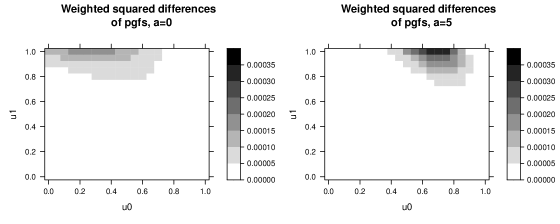
Figure 1. Heatmaps of the weighted squared difference of the two estimated pgfs for an INGARCH$(1,1)$ DGP (left: $a=0$, right: $a=5$).

Table 4. Power in case of a Poi($\lambda$)-INAR(2) DGP when testing for $H_{0}^{\text{semi}}$ in (1.4) with $p=1$. Numbers in italic are taken from Table 1 in [27] who test for $H_{0}^{\text{para}}$ in (1.3) with $p=1$ and $G_{\lambda}$=Poi($\lambda$).

			$a=0$		$a=5$		$a=2$		MK, $a=2$
$\lambda$	$\alpha_{1}$	$\alpha_{2}$	$n=100$	$n=500$	$n=100$	$n=500$	$n=100$	$n=500$	$n=100$	$n=500$
1	0.3	0.1	0.039	0.046	0.045	0.050	0.040	0.043	0.088	0.035
1	0.5	0.1	0.044	0.063	0.056	0.104	0.050	0.086	0.089	0.127
1	0.5	0.3	0.097	0.206	0.178	0.525	0.144	0.415	0.191	0.487

Table 5. Power in case of an INGARCH$(1,1)$ DGP when testing for $H_{0}^{\text{semi}}$ in (1.4) with $p=1$. Numbers in italic are taken from Table 1 in [27] who test for $H_{0}^{\text{para}}$ in (1.3) with $p=1$ and $G_{\lambda}$=Poi($\lambda$).

				$a=0$		$a=5$		$a=2$		MK, $a=2$
$\beta_{0}$	$\beta_{1}$	$\alpha_{1}$	$\rho(1)$	$n=100$	$n=500$	$n=100$	$n=500$	$n=100$	$n=500$	$n=100$	$n=500$
0.2	0.4	0.10	0.09	0.026	0.018	0.026	0.030	0.023	0.021	0.012	0.050
0.2	0.4	0.20	0.21	0.031	0.087	0.054	0.131	0.044	0.117	0.042	0.108
1.0	0.1	0.50	0.52	0.068	0.205	0.159	0.645	0.113	0.501	0.152	0.512
0.5	0.1	0.50	0.52	0.177	0.707	0.256	0.865	0.237	0.833	0.248	0.724
0.1	0.4	0.40	0.53	0.264	0.829	0.255	0.816	0.264	0.825	0.296	0.902
0.6	0.1	0.60	0.66	0.271	0.881	0.446	0.982	0.399	0.969	0.376	0.988
0.1	0.2	0.60	0.70	0.497	0.985	0.443	0.973	0.468	0.980	0.534	0.998
0.1	0.5	0.45	0.78	0.526	0.997	0.542	0.996	0.562	0.997	0.669	0.986

An additional explanation for the generally rather low power values is that when testing the null of an INAR(1) process, we consider the pgf of order 1. However, this does not explain the entire dependence structure of an alternative Poi-INAR(2) or INGARCH$(1,1)$ process, since both of them are no first-order Markov chains. To address this, we fit an INAR(1) model to the DGP but now use the second-order test statistic $T_{n}^{(2)}$ ($s=2$ in (2.10)) by setting $\widehat{\alpha}_{\text{sp},2}:=0$ as suggested in Remark 2.2. The size results are presented in Tables 6 and 7, where we see that we still keep the level of $5\%$. Tables 8 and 9 contain the resulting power values. For comparison, we again included the power values of [27] in italics, which still result from using the first-order test statistic ($p=1$ in (2.8)). As anticipated, the power of the second-order test statistics increased, in some settings substantially. Again, we tend to achieve higher power values with higher weighting.

Table 6. Actual sizes in case of a Poi($\lambda$)-INAR(1) DGP when testing for $H_{0}^{\text{semi}}$ in (1.4) with $p=1$ using test statistic (2.10) with $s=2$. Numbers in italic display the power values taken from Table 1 in [27] who test for $H_{0}^{\text{para}}$ in (1.3) with $p=1$ and $G_{\lambda}$=Poi($\lambda$) not using a higher-order test statistic analogously to (2.10).

		$a=0$		$a=5$		$a=2$		MK, $a=2$
$\lambda$	$\alpha$	$n=100$	$n=500$	$n=100$	$n=500$	$n=100$	$n=500$	$n=100$	$n=500$
1	0.3	0.047	0.047	0.047	0.041	0.044	0.044	0.049	0.055
1	0.5	0.039	0.047	0.042	0.051	0.038	0.050	0.051	0.053
3	0.3	0.027	0.035	0.048	0.036	0.042	0.037	0.056	0.047
3	0.5	0.027	0.030	0.043	0.037	0.038	0.037	0.055	0.059

Table 7. Actual sizes in case of a NB($N,\pi$)-INAR(1) DGP when testing for $H_{0}^{\text{semi}}$ in (1.4) with $p=1$ using test statistic (2.10) with $s=2$. Numbers in italic display the power values taken from Table 1 in [27] who test for $H_{0}^{\text{para}}$ in (1.3) with $p=1$ and $G_{\lambda}$=Poi($\lambda$) not using a higher-order test statistic analogously to (2.10).

			$a=0$		$a=5$		$a=2$		MK, $a=2$
$N$	$\pi$	$\alpha$	$n=100$	$n=500$	$n=100$	$n=500$	$n=100$	$n=500$	$n=100$	$n=500$
1	0.500	0.5	0.053	0.053	0.052	0.051	0.053	0.052	0.686	1.000
2	0.667	0.5	0.046	0.050	0.048	0.050	0.049	0.050	0.327	0.897
10	0.909	0.5	0.045	0.044	0.047	0.047	0.045	0.041	0.120	0.149

Table 8. Power in case of a Poi($\lambda$)-INAR(2) DGP when testing for $H_{0}^{\text{semi}}$ in (1.4) with $p=1$ using test statistic (2.10) with $s=2$. Numbers in italic display the power values taken from Table 1 in [27] who test for $H_{0}^{\text{para}}$ in (1.3) with $p=1$ and $G_{\lambda}$=Poi($\lambda$) not using a higher-order test statistic analogously to (2.10).

			$a=0$		$a=5$		$a=2$		MK, $a=2$
$\lambda$	$\alpha_{1}$	$\alpha_{2}$	$n=100$	$n=500$	$n=100$	$n=500$	$n=100$	$n=500$	$n=100$	$n=500$
1	0.3	0.1	0.068	0.205	0.079	0.391	0.082	0.354	0.088	0.035
1	0.5	0.1	0.060	0.141	0.080	0.311	0.072	0.251	0.089	0.127
1	0.5	0.3	0.114	0.401	0.328	0.958	0.240	0.848	0.191	0.487

Table 9. Power in case of an INGARCH$(1,1)$ DGP when testing for $H_{0}^{\text{semi}}$ in (1.4) with $p=1$ using test statistic (2.10) with $s=2$. Numbers in italic display the power values taken from Table 1 in [27] who test for $H_{0}^{\text{para}}$ in (1.3) with $p=1$ and $G_{\lambda}$=Poi($\lambda$) not using a higher-order test statistic analogously to (2.10).

				$a=0$		$a=5$		$a=2$		MK, $a=2$
$\beta_{0}$	$\beta_{1}$	$\alpha_{1}$	$\rho(1)$	$n=100$	$n=500$	$n=100$	$n=500$	$n=100$	$n=500$	$n=100$	$n=500$
0.2	0.4	0.10	0.09	0.045	0.101	0.052	0.119	0.048	0.116	0.012	0.050
0.2	0.4	0.20	0.21	0.090	0.403	0.099	0.449	0.100	0.467	0.042	0.108
1.0	0.1	0.50	0.52	0.068	0.178	0.166	0.691	0.123	0.528	0.152	0.512
0.5	0.1	0.50	0.52	0.141	0.628	0.249	0.884	0.222	0.846	0.248	0.724
0.1	0.4	0.40	0.53	0.449	0.989	0.366	0.970	0.416	0.983	0.296	0.902
0.6	0.1	0.60	0.66	0.216	0.812	0.440	0.987	0.376	0.973	0.376	0.988
0.1	0.2	0.60	0.70	0.566	0.996	0.489	0.989	0.534	0.994	0.534	0.998
0.1	0.5	0.45	0.78	0.697	1.000	0.717	1.000	0.749	1.000	0.669	0.986

The parametric testing approaches as in [27] allow to test for deviations from the null in terms of model order, which can also be done with our semi-parametric goodness-of-fit test. In addition, due to the flexible and non-restrictive nature of the null hypothesis (1.4), we are able to test for deviations from the INAR structure in general. For this purpose, we consider INARCH(1) and Poi-DAR(1) DGPs with different parametrizations, see [34]. Both exhibit an autoregressive structure of order 1 but distinct from an INAR. The INARCH(1) process is a special case of the INGARCH$(1,1)$ process, i.e. $X_{t}|X_{t-1},X_{t-2},\ldots\sim\text{Poi($M_{t}$), where $M_{t}=\beta+\alpha X_{t-1}$}$. A Poi-DAR(1) process is characterized by $X_{t}=aX_{t-1}+b\varepsilon_{t}$, where $\varepsilon_{t}\overset{\text{i.i.d.}}{\sim}$ Poi($\lambda$) and $(a,b)\sim\text{Mult}(1,\alpha,1-\alpha)$. In this latter model class, each observation either chooses the previous observation or an innovation, so the stationary marginal distribution of the innovations equals that of the observations. We choose such values for $\lambda$ and $\beta$ to obtain similar observation means as for the other DGPs. For both DGPs, INARCH(1) and Poi-DAR(1), the power is larger for higher autocorrelation levels (provided that $a>0$), see Tables 10 and 11. This is plausible since for high autocorrelation (and small innovation mean), an INAR(1) process tends to produce “runs”, i.e. same observation in consecutive time points. In contrast, the INARCH(1) model shows more erratic behavior. The Poi-DAR(1) process, on the other hand, exhibits even more extreme runs with higher autocorrelation combined with further “jumps” in-between these runs.

Table 10. Power in case of an INARCH(1) DGP when testing for $H_{0}^{\text{semi}}$ in (1.4) with $p=1$.

		$a=0$		$a=5$		$a=2$
$\beta$	$\alpha$	$n=100$	$n=500$	$n=100$	$n=500$	$n=100$	$n=500$
1	0.30	0.032	0.044	0.048	0.129	0.039	0.094
1	0.50	0.071	0.264	0.159	0.658	0.119	0.540
1	0.75	0.271	0.914	0.604	0.999	0.506	0.997
3	0.30	0.035	0.030	0.046	0.022	0.038	0.025
3	0.50	0.025	0.028	0.052	0.054	0.037	0.034
3	0.75	0.074	0.184	0.185	0.634	0.133	0.460

Table 11. Power in case of a Poi($\lambda$)-DAR DGP when testing for $H_{0}^{\text{semi}}$ in (1.4) with $p=1$.

		$a=0$		$a=5$		$a=2$
$\lambda$	$\alpha$	$n=100$	$n=500$	$n=100$	$n=500$	$n=100$	$n=500$
2	0.25	0.144	0.437	0.115	0.226	0.117	0.212
2	0.50	0.447	0.992	0.535	0.995	0.538	0.994
2	0.75	0.326	0.982	0.400	0.997	0.401	0.996
6	0.25	0.142	0.279	0.160	0.159	0.163	0.230
6	0.50	0.117	0.371	0.234	0.707	0.190	0.643
6	0.75	0.016	0.041	0.277	0.980	0.121	0.920

While we have high power in most scenarios, we also encounter some parametrizations with low power, e.g. for INARCH(1) processes with low autocorrelation $\alpha$ and high intercept $\beta$. In general, we seem to lose power for increasing mean of observations (due to additive terms rather than increasing autocorrelation). A higher observation mean leads to a wider range of observations, potentially affecting both the semi-parametric and the non-parametric estimation of the pgf, where the latter is also included in the parametric testing approaches. Besides the challenges related to semi- and non-parametric estimation, the considered DGPs themselves may contribute to low power results. As mentioned at the begin of our paper, without restraining to a certain parametric family of innovations, the INAR model class is very flexible, the unspecified innovation distribution presents a high degree of freedom. Consider for example the INARCH(1) DGP with $\beta=3$ and $\alpha=0.3$ which leads to low power results as displayed in Table 10. Additionally, consider an INGARCH$(1,1)$ DGP with $\beta_{0}=0.6$, $\beta_{1}=0.1$ and $\alpha_{1}=0.6$ which leads to good power results as displayed in Table 5. For both DGPs, we simulated a sample of $n=5000$ observations and computed the integrand of (2.8), $\Big{(}\widehat{g}_{1;H_{0}}(u_{0},u_{1})-\widehat{g}_{1}(u_{0},u_{1})\Big{)}^{2}$, for $u_{0},u_{1}\in\{0,0.05,0.1,\ldots,1\}$. For the sake of comparison, we also considered an INAR(1) DGP with $\lambda=3$ and $\alpha=0.3$. Figure 2 shows the boxplots of the resulting values for the three different DGPs. While the two-dimensional pgf of order 1, i.e., $g_{2}$, of the considered INGARCH$(1,1)$ DGP differs much from the one of a semi-parametrically estimated INAR(1) process, the first-order pgf of the considered INARCH(1) DGP is very close to the latter. Actually, $\widehat{g}_{1;H_{0}}(u_{0},u_{1})$ and $\widehat{g}_{1}(u_{0},u_{1})$ do not differ much, the differences are even as small as for the considered INAR(1) DGP. This explains the low power results and underlines the flexibility of the INAR model with unspecified innovation distribution.

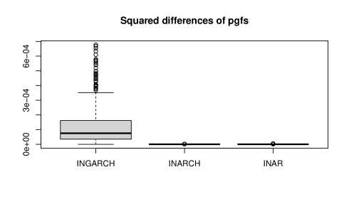
Figure 2. Boxplots of the squared differences of the two estimated pgfs for the considered INGARCH (left), INARCH (middle) and INAR (right) DGPs.

In summary, under the null, it becomes clear that we achieve better results when there is no weighting of the test statistic. However, since a higher weighting of the test statistic leads to substantially higher power values under the alternative and we still keep the level under the null using higher weighting, we recommend using the test with a comparatively high weighting, i.e. ${a=5}$.

5. Real-World Data Applications

To illustrate the application of our proposed goodness-of-fit test, we apply it on three economic real-world data examples using $B=1000$ bootstrap repetitions.

The first data set is sourced from Baker Hughes containing weekly counts of active rotary drilling rigs. These counts serve as indicator for the demand of products used in drilling, well completion, oil production, and hydrocarbon processing and have been published since 1944. We specifically focus on the number of drilling rigs in Alaska from 1991 to 1997 ($n=417$). This data set has been addressed before in [34]. Figure 3 shows a plot of the time series and the corresponding ACF and PACF. The characteristic INAR runs suggest a high serial dependence with small innovation mean, which are confirmed by the high and slowly decreasing autocorrelation level. Looking at the partial autocorrelation function (PACF), an AR(1)-like model seems to be an appropriate fit. Indeed, when applying our test $T_{n}$ on the data using $a=5$, we do not reject the null of an INAR(1) process at $5\%$ level.

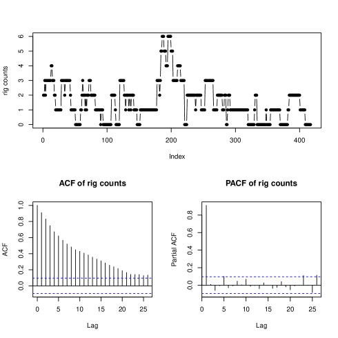
Figure 3. Plot of rig counts and the corresponding (P)ACF.

The second data set was provided by the Deutsche Börse Group and has been discussed before in [17]. It contains counts per trading day of transactions of structured products between February 2017 and August 2019 ($n=404$). The data are displayed in Figure 4. As in the previous example of rig counts, the ACF and PACF suggest that an INAR(1) model might be an appropriate fit for the data. But applying the test of [27], it rejects the null of a Poi-INAR(1) model at $5\%$ level ($a=2$). Our test, by contrast, also using $a=2$, does not reject the INAR(1) null at $5\%$ level. These different results may be explained by the dispersion of the data. With $\bar{x}\approx 1.47$ and $s^{2}\approx 2.23$, the index of dispersion is approximately 1.51 suggesting overdispersed counts. This is additionally stressed out by Figure 5. It displays the semi-parametric (left plot) and parametric estimation of the innovation distribution, where for the latter we used a Poisson distribution (in the middle) and a geometric distribution (on the right), respectively. We see that the parametrically estimated (equidispersed) Poisson distribution differs much from the semi-parametrically estimated innovation distribution whereas the (overdispersed) geometric distribution seems much more appropriate as innovation distribution. Hence, while the parametric test of [27] fails to detect the INAR model structure due to their too restrictive equidispersion property of the data under the null, our more flexible test does not reject the INAR structure.

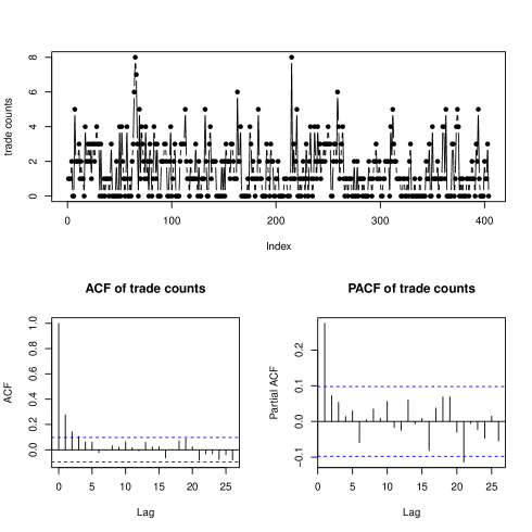
Figure 4. Plot of daily trade counts and the corresponding (P)ACF.

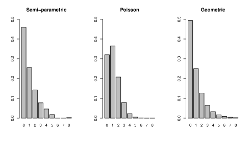
Figure 5. Plot of the semi-parametrically (left) and parametrically (Poisson in the middle, Geometric on the right) estimated innovation distribution.

In our third application, we consider a data set first published by [6]. It records the number of transaction of the Ericsson B stock per minute between 9:35 and 17:44. Originally, it provides data for the days between July 2 and 22, 2002. [14], [35], [7], [8] and [34] exclusively consider the data of July 2 and model the data by an INGARCH$(1,1)$ process. The resulting time series is of length $n=460$. Figure 6 shows a plot of this time series along with the corresponding (P)ACF. By contrast to the first two examples, this data set exhibits a more erratic structure. The ACF is slowly decaying and the PACF suggests dependencies of higher order than 1. Applying our goodness-of-fit test to the null $H_{0}^{\text{semi}}$ in (1.4) with $p=1$, we are initially not able to reject the null at level $5\%$. However, when using the second-order test statistic $T_{n}^{(2)}$ ($s=2$ in (2.10)), we ultimately reject the null (both with $a=5$). This is plausible since we capture dependencies of higher order by considering the three-dimensional pgf of order 2, i.e., $g_{2}$, instead of the two-dimensional pgf of order 1, i.e., $g_{1}$.

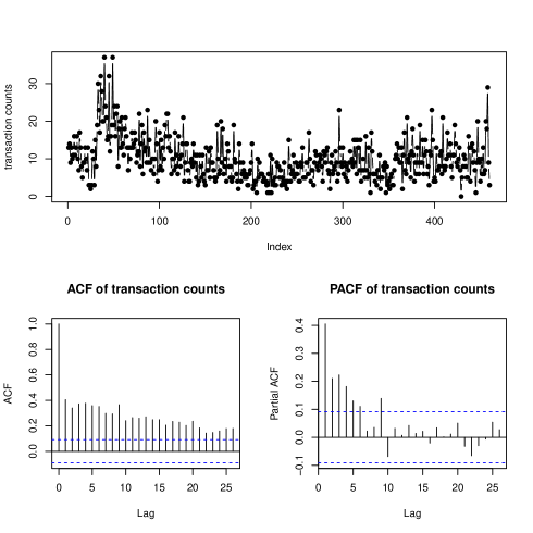
Figure 6. Plot of transaction counts and the corresponding (P)ACF.

6. Conclusion

In existing literature, goodness-of-fit tests for the INAR model class are restricted to specific parametric families of innovation distributions. In this paper, we introduced a novel goodness-of-fit test for INAR($p$) processes that does not rely on parametric assumptions about the nature of the innovations. We derived the null limiting distribution of our $L_{2}$-type test statistic based on weighted integrals using probability generating functions. Additionally, we proved its consistency under fixed alternatives, discussed the asymptotic behavior under local alternatives, and specified a bootstrap procedure required to circumvent the complex limiting distribution. In an extensive simulation study, we compared our proposed procedure with the parametric competitor of [27]. Overall, we got similar results, but we were able to increase the power against Markov chain alternatives of higher order by using also higher-order test statistics. Moreover, unlike the parametric approaches of [27], we are able to test for general deviations from the INAR structure and got good power results for the considered DGPs. We noticed that when testing with higher weight parameter $a$, the test exhibited higher power. To conclude the paper, we applied our method to three real data examples from economics.

References

Appendix A Proofs

A.1. Proof of Lemma 2.1

Exploiting the INAR($p$) model structure of $X_{t},\ldots,X_{t-p}$, we get

$$E\left(\prod_{j=0}^{p}u_{j}^{X_{t-j}}\right) =E\left(E\left(\prod_{j=0}^{p}u_{j}^{X_{t-j}}|X_{t-1},\ldots,X_{t-p}\right)\right)$$

$$=E\left(\prod_{j=1}^{p}u_{j}^{X_{t-j}}E\left(u_{0}^{X_{t}}|X_{t-1},\ldots,X_{t-p}\right)\right).$$

Taking a closer look at the interior conditional expectation and inserting the model equation, we get

$$E\left(u_{0}^{X_{t}}|X_{t-1},\ldots,X_{t-p}\right) =E\left(u_{0}^{\alpha_{1}\circ X_{t-1}+\cdots+\alpha_{p}\circ X_{t-p}+\varepsilon_{t}}|X_{t-1},\ldots,X_{t-p}\right)$$

$$=\left\{\prod_{i=1}^{p}E\left(u_{0}^{\alpha_{i}\circ X_{t-i}}|X_{t-1},\ldots,X_{t-p}\right)\right\}\cdot E(u_{0}^{\varepsilon_{t}})$$

$$=\left\{\prod_{i=1}^{p}E\left(u_{0}^{\alpha_{i}\circ X_{t-i}}|X_{t-i}\right)\right\}\cdot E(u_{0}^{\varepsilon_{t}})$$

$$=\left\{\prod_{i=1}^{p}\Big{(}1+\alpha_{i}(u_{0}-1)\Big{)}^{X_{t-i}}\right\}\cdot g_{\varepsilon}(u_{0}),$$

where we have used that given $X_{t-1},\ldots,X_{t-p}$, the thinning operations and the innovation $\varepsilon_{t}$ are independent. The thinning operation $\alpha_{i}\circ$ only depends on $X_{t-i}$ and $\alpha_{i}\circ X_{t-i}|X_{t-i}\sim\text{Bin}(X_{t-i},\alpha_{i})$ together with the well-known formula for the pgf of a binomial distribution. Furthermore, we define $g_{\varepsilon}(u_{0}):=E(u_{0}^{\varepsilon_{t}})$ as the marginal pgf of the innovations. Hence, we get the following representation for the joint pgf of $X_{t},\ldots,X_{t-p}$:

$$g_{p}(u_{0},\ldots,u_{p}) :=E\left(\prod_{j=0}^{p}u_{j}^{X_{t-j}}\right)$$

$$=E\left(\prod_{j=1}^{p}u_{j}^{X_{t-j}}\left\{\prod_{i=1}^{p}(1+\alpha_{i}(u_{0}-1))^{X_{t-i}}\right\}\cdot g_{\varepsilon}(u_{0})\right)$$

$$=g_{\varepsilon}(u_{0})\cdot E\left(\prod_{j=1}^{p}u_{j}^{X_{t-j}}\left\{\prod_{i=1}^{p}(1+\alpha_{i}(u_{0}-1))^{X_{t-i}}\right\}\right)$$

$$=g_{\varepsilon}(u_{0})\cdot E\left(\prod_{j=1}^{p}\Big{\{}u_{j}\big{(}1+\alpha_{j}(u_{0}-1)\big{)}\Big{\}}^{X_{t-j}}\right).$$

$\square$

A.2. Proof of Lemma 2.3

Plugging-in (2.5) and (2.7) and rearranging terms, we get

$$T_{n}= n\int_{0}^{1}\cdots\int_{0}^{1}\Big{(}\widehat{g}_{p;H_{0}}(u_{0},\ldots,u_{p})-\widehat{g}_{p}(u_{0},\ldots,u_{p})\Big{)}^{2}\,w(u_{0},\ldots,u_{p};a)\,du_{0}\cdots du_{p}$$

$$= \frac{n}{(n-p)^{2}}(a+1)^{p+1}\,\sum_{t,s=p+1}^{n}\int_{0}^{1}\cdots\int_{0}^{1}\left(\prod_{j=1}^{p}u_{j}^{X_{t-j}}\right)\left(\prod_{j=1}^{p}u_{j}^{X_{s-j}}\right)\,\left(\prod\limits_{j=1}^{p}u_{j}^{a}\right)\,du_{1}\cdots du_{p}$$

$$\times\int_{0}^{1}\left(u_{0}^{X_{t}}-\widehat{g}_{\varepsilon}(u_{0})\,\prod_{j=1}^{p}\big{(}1+\widehat{\alpha}_{\text{sp},j}(u_{0}-1)\big{)}^{X_{t-j}}\right)$$

$$\left(u_{0}^{X_{s}}-\widehat{g}_{\varepsilon}(u_{0})\,\prod_{j=1}^{p}\big{(}1+\widehat{\alpha}_{\text{sp},j}(u_{0}-1)\big{)}^{X_{s-j}}\right)\,u_{0}^{a}\,du_{0}$$

$$= \frac{n}{(n-p)^{2}}(a+1)^{p+1}\,\sum_{t,s=p+1}^{n}\left(\prod_{j=1}^{p}\int_{0}^{1}u_{j}^{X_{t-j}+X_{s-j}+a}du_{j}\right)$$

$$\times\int_{0}^{1}\Biggl{(}u_{0}^{X_{t}+X_{s}+a}+\widehat{g}_{\varepsilon}(u_{0})^{2}\,u_{0}^{a}\,\prod_{j=1}^{p}\big{(}1+\widehat{\alpha}_{\text{sp},j}(u_{0}-1)\big{)}^{X_{t-j}+X_{s-j}}$$

$$-\widehat{g}_{\varepsilon}(u_{0})\,u_{0}^{X_{s}+a}\prod_{j=1}^{p}\big{(}1+\widehat{\alpha}_{\text{sp},j}(u_{0}-1)\big{)}^{X_{t-j}}-\widehat{g}_{\varepsilon}(u_{0})\,u_{0}^{X_{t}+a}\prod_{j=1}^{p}\big{(}1+\widehat{\alpha}_{\text{sp},j}(u_{0}-1)\big{)}^{X_{s-j}}\Biggl{)}\,du_{0}.$$

Further, by using that

$$\int_{0}^{1}u^{x}\,du=1/(1+x)$$ (A.1)

holds for $x\not=-1$, $T_{n}$ can be simplified to get

$$T_{n}= \frac{n}{(n-p)^{2}}(a+1)^{p+1}\,\sum_{t,s=p+1}^{n}\left(\prod_{j=1}^{p}\frac{1}{1+X_{t-j}+X_{s-j}+a}\right)$$

$$\times\left(\frac{1}{1+X_{t}+X_{s}+a}+\int_{0}^{1}\widehat{g}_{\varepsilon}(u_{0})^{2}u_{0}^{a}\,\prod_{j=1}^{p}\big{(}1+\widehat{\alpha}_{\text{sp},j}(u_{0}-1)\big{)}^{X_{t-j}+X_{s-j}}du_{0}\right.$$

$$\left.-2\int_{0}^{1}\widehat{g}_{\varepsilon}(u_{0})\,u_{0}^{X_{s}+a}\prod_{j=1}^{p}\big{(}1+\widehat{\alpha}_{\text{sp},j}(u_{0}-1)\big{)}^{X_{t-j}}du_{0}\right).$$

To be able to use the same integration rule A.1 also for the two remaining integrals above, we need to isolate the terms in $u_{0}$. On the one hand, we have

$$\widehat{g}_{\varepsilon}(u_{0})^{2}=\sum\limits_{k_{1},k_{2}=0}^{\max(X_{1},\ldots,X_{n})}\widehat{G}_{\text{sp}}(k_{1})\widehat{G}_{\text{sp}}(k_{2})u_{0}^{k_{1}+k_{2}}.$$

By using twice the binomial theorem in each case, on the other hand, we get

$$(1+\widehat{\alpha}_{\text{sp},j}(u_{0}-1))^{X_{t-j}+X_{s-j}}=\sum\limits_{i_{j}=0}^{X_{t-j}+X_{s-j}}\binom{X_{t-j}+X_{s-j}}{i_{j}}\widehat{\alpha}_{\text{sp},j}^{i_{j}}\sum\limits_{h_{j}=0}^{i_{j}}\binom{i_{j}}{h_{j}}u_{0}^{h_{j}}(-1)^{i_{j}-h_{j}}$$

and

$$(1+\widehat{\alpha}_{\text{sp},j}(u_{0}-1))^{X_{t-j}}=\sum\limits_{i_{j}=0}^{X_{t-j}}\binom{X_{t-j}}{i_{j}}\widehat{\alpha}_{\text{sp},j}^{i_{j}}\sum\limits_{h_{j}=0}^{i_{j}}\binom{i_{j}}{h_{j}}u_{0}^{h_{j}}(-1)^{i_{j}-h_{j}},$$

respectively. Altogether, this leads to

$$T_{n} =\frac{n}{(n-p)^{2}}(a+1)^{p+1}\left(\prod\limits_{j=1}^{p}\frac{1}{1+X_{t-j}+X_{s-j}+a}\right)\Bigg{[}\frac{1}{1+X_{t}+X_{s}+a}$$

$$+\sum\limits_{k_{1},k_{2}=0}^{\max(X_{1},\ldots,X_{n})}\widehat{G}_{\text{sp}}(k_{1})\widehat{G}_{\text{sp}}(k_{2})\sum\limits_{i_{1}=0}^{X_{t-1}+X_{s-1}}\sum\limits_{h_{1}=0}^{i_{1}}\ldots\sum\limits_{i_{p}=0}^{X_{t-p}+X_{s-p}}\sum\limits_{h_{p}=0}^{i_{p}}$$

$$\prod\limits_{j=1}^{p}\binom{X_{t-j}+X_{s-j}}{i_{j}}\widehat{\alpha}_{\text{sp},j}^{i_{j}}(-1)^{i_{j}-h_{j}}\binom{i_{j}}{h_{j}}\int\limits_{0}^{1}u_{0}^{1+k_{1}+k_{2}+a+\sum_{m=1}^{p}h_{m}}du_{0}-2\sum\limits_{k=0}^{\max(X_{1},\ldots,X_{n})}\widehat{G}_{\text{sp}}(k)$$

$$\sum\limits_{i_{1}=0}^{X_{t-1}+X_{s-1}}\sum\limits_{h_{1}=0}^{i_{1}}\ldots\sum\limits_{i_{p}=0}^{X_{t-p}+X_{s-p}}\sum\limits_{h_{p}=0}^{i_{p}}\prod\limits_{j=1}^{p}\binom{X_{t-j}}{i_{j}}\widehat{\alpha}_{\text{sp},j}^{i_{j}}(-1)^{i_{j}-h_{j}}\binom{i_{j}}{h_{j}}\int\limits_{0}^{1}u_{0}^{1+k+X_{s}+a+\sum_{m=1}^{p}h_{m}}du_{0}\Bigg{]}.$$

Applying (A.1), the assertion follows. $\square$

A.3. Proof of Proposition 2.4

The only aspect that remains to show is the degeneracy. Let $h$ be the kernel defined in (2.12). Using $y_{t}=(x_{t},\ldots,x_{t-p})\in\mathbb{N}_{0}^{p+1}$, under the null $H_{0}^{semi}(\theta_{0})$ in (2.11), we have

$$E(h(y_{t},Y_{s};\theta_{0})) =\int\limits_{0}^{1}\ldots\int\limits_{0}^{1}\left(g_{0,\varepsilon}(u_{0})\prod\limits_{j=1}^{p}(u_{j}(1+\alpha_{0,j}(u_{0}-1)))^{x_{t-j}}-\prod\limits_{j=0}^{p}u_{j}^{x_{t-j}}\right)$$

$$\quad\quad\quad\quad\times E\left(g_{0,\varepsilon}(u_{0})\prod\limits_{j=1}^{p}(u_{j}(1+\alpha_{0,j}(u_{0}-1)))^{X_{s-j}}-\prod\limits_{j=0}^{p}u_{j}^{X_{s-j}}\right)$$

$$\quad\quad\quad\quad w(u_{0},\ldots,u_{p};a)\,du_{0}\ldots du_{p}$$

$$=\int\limits_{0}^{1}\ldots\int\limits_{0}^{1}\left(g_{0,\varepsilon}(u_{0})\prod\limits_{j=1}^{p}(u_{j}(1+\alpha_{0,j}(u_{0}-1)))^{x_{t-j}}-\prod\limits_{j=0}^{p}u_{j}^{x_{t-j}}\right)$$

$$\quad\quad\quad\quad\quad\times\Big{(}pgf_{H_{0}}(X_{s},\ldots,X_{s-p})-pgf(X_{s},\ldots,X_{s-p})\Big{)}$$

$$\quad\quad\quad\quad w(u_{0},\ldots,u_{p};a)\,du_{0}\ldots du_{p}$$

$$=0,$$

because $pgf_{H_{0}}(X_{s},\ldots,X_{s-p})=pgf(X_{s},\ldots,X_{s-p})$ under $H_{0}^{semi}(\theta_{0})$. That is, we are in the case of a degenerate kernel. $\square$

A.4. Proof of Theorem 2.5

Using Proposition 2.4, we already have the degeneracy of the kernel (2.12). In view of Theorem 1 in [24], under $H_{0}^{semi}(\theta_{0})$, the kernel $h$ even fulfills the stronger degeneracy condition

$$E(h(y_{t},Y_{s};\theta_{0})|Y_{1},\ldots,Y_{s-1})$$

$$=\int\limits_{0}^{1}\ldots\int\limits_{0}^{1}\left(g_{0,\varepsilon}(u_{0})\prod\limits_{j=1}^{p}(u_{j}(1+\alpha_{0,j}(u_{0}-1)))^{x_{t-j}}-\prod\limits_{j=0}^{p}u_{j}^{x_{t-j}}\right)$$ (A.2)

$$\quad\quad\times E\left(g_{0,\varepsilon}(u_{0})\prod\limits_{j=1}^{p}(u_{j}(1+\alpha_{0,j}(u_{0}-1)))^{X_{s-j}}-\prod\limits_{j=0}^{p}u_{j}^{X_{s-j}}|Y_{1},\ldots,Y_{s-1}\right)$$

$$\quad\quad\quad\quad w(u_{0},\ldots,u_{p};a)\,du_{0}\ldots du_{p}$$

$$=0.$$

By using the Markov property of an INAR process, this is the case, because

$$\quad\quad E\left(g_{0,\varepsilon}(u_{0})\prod\limits_{j=1}^{p}(u_{j}(1+\alpha_{0,j}(u_{0}-1)))^{X_{s-j}}-\prod\limits_{j=0}^{p}u_{j}^{X_{s-j}}|Y_{1},\ldots,Y_{s-1}\right)$$

$$=E\left(g_{0,\varepsilon}(u_{0})\prod\limits_{j=1}^{p}(u_{j}(1+\alpha_{0,j}(u_{0}-1)))^{X_{s-j}}-\prod\limits_{j=0}^{p}u_{j}^{X_{s-j}}|X_{1-p},\ldots,X_{s-1}\right)$$

$$=E\left(g_{0,\varepsilon}(u_{0})\prod\limits_{j=1}^{p}(u_{j}(1+\alpha_{0,j}(u_{0}-1)))^{X_{s-j}}|X_{1-p},\ldots,X_{s-1}\right)-E\left(\prod\limits_{j=0}^{p}u_{j}^{X_{s-j}}|X_{1-p},\ldots,X_{s-1}\right)$$

$$=g_{0,\varepsilon}(u_{0})\prod\limits_{j=1}^{p}(u_{j}(1+\alpha_{0,j}(u_{0}-1)))^{X_{s-j}}-\prod\limits_{j=1}^{p}u_{j}^{X_{s-j}}E(u_{0}^{X_{s}}|X_{1-p},\ldots,X_{s-1})$$

$$=g_{0,\varepsilon}(u_{0})\prod\limits_{j=1}^{p}(u_{j}(1+\alpha_{0,j}(u_{0}-1)))^{X_{s-j}}-\prod\limits_{j=1}^{p}u_{j}^{X_{s-j}}g_{0,\varepsilon}(u_{0})\prod\limits_{j=1}^{p}(1+\alpha_{0,j}(u_{0}-1))^{X_{s-j}}$$

$$=0,$$

where we used the null $H_{0}^{semi}(\theta_{0})$ to get $E(u_{0}^{X_{s}}|X_{1-p},\ldots,X_{s-1})=g_{0,\varepsilon}(u_{0})\prod\limits_{j=1}^{p}(1+\alpha_{0,j}(u_{0}-1))^{X_{s-j}}$.

Furthermore, because the kernel $h$ is of a quadratic form, it is positive semidefinite. That is, for all $m\in\mathbb{N}$ and for all $c_{1},\ldots,c_{m}\in\mathbb{R},\,y_{1},\ldots,y_{m}\in\mathbb{N}_{0}^{p+1}$, it holds $\sum_{t,s=1}^{m}c_{t}c_{s}h(y_{t},y_{s})\geq 0$. Moreover, because all the terms of the integrand, i.e., $g_{\varepsilon}(u_{0}),u_{0},\ldots,u_{p},\alpha_{1},\ldots,\alpha_{p}$, are bounded by 0 from below and by 1 from above, we have

$$E(h(Y_{0},Y_{0};\theta_{0})) =\int\limits_{0}^{1}\ldots\int\limits_{0}^{1}E\left(\left(g_{0,\varepsilon}(u_{0})\prod\limits_{j=1}^{p}(u_{j}(1+\alpha_{0,j}(u_{0}-1)))^{X_{t-j}}-\prod\limits_{j=0}^{p}u_{j}^{X_{t-j}}\right)^{2}\right)$$

$$\quad\quad\quad\quad w(u_{0},\ldots,u_{p};a)\,du_{0}\ldots du_{p}$$

$$<\infty.$$

With $(X_{t})_{t\in\mathbb{Z}}$ being a strictly stationary and ergodic process [11], we can apply Theorem 1 of [24]. Precisely, under the null $H_{0}^{semi}(\theta_{0})$ and for $n\rightarrow\infty$, this leads to

$$T_{n}(\theta_{0})\overset{d}{\longrightarrow}\sum\limits_{k=1}^{\infty}\lambda_{k}Z_{k}^{2},$$

where $(Z_{k})_{k}$ is a sequence of independent standard normal random variables and $(\lambda_{k})_{k}$ the sequence of nonzero eigenvalues of (2.13) enumerated according their multiplicity with $(\Phi_{k})_{k}$ the associated orthonormal eigenfunctions. $\square$

A.5. Proof of Theorem 2.6

Let $\theta_{0}=(\boldsymbol{\alpha}_{0},G_{0})\in A\times\mathcal{G}$ denote the true parameter. For any $\theta\in\Theta$, we see that the kernel $h$ can be represented as

$$h(x,y;\theta)=\int_{[0,1]^{p+1}}h_{1}(x,\mathbf{u};\theta)h_{1}(y,\mathbf{u};\theta)Q(d\mathbf{u}),$$

where $\mathbf{u}=(u_{0},\ldots,u_{p})$, $h_{1}:\mathbb{R}^{p+1}\times[0,1]^{p+1}\times\Theta\rightarrow\mathbb{R}$, $\Theta=(0,1)^{p}\times\mathcal{G}$ with

$$h_{1}(y_{t},\mathbf{u};\theta)=g_{\varepsilon}(u_{0})\prod\limits_{j=1}^{p}(u_{j}(1+\alpha_{j}(u_{0}-1)))^{x_{t-j}}-\prod\limits_{j=0}^{p}u_{j}^{x_{t-j}}$$ (A.3)

with $y_{t}=(x_{t},\ldots,x_{t-p})$ and the probability measure $Q$ has probability density function $w$, that is, $dQ/d\mathbf{u}=w(\mathbf{u})$. Using that both terms of the difference in (A.3) only take values in $[0,1]$, $\boldsymbol{\alpha}\in(0,1)^{p}$, $G\in\mathcal{G}$ and that the integration limits of all the following integrals are 0 and 1, we see that (A.3) fulfills

$$\int\limits_{[0,1]^{p+1}}h_{1}(y,\mathbf{u};\theta_{0})^{2}Q(d\mathbf{u})<\infty,\quad\int\limits_{[0,1]^{p+1}}E_{\theta_{0}}\left(h_{1}(Y_{0},\mathbf{u};\theta_{0})^{2}\right)Q(d\mathbf{u})<\infty$$

as well as the continuity condition

$$\int\limits_{[0,1]^{p+1}}\big{(}h_{1}(y,\mathbf{u};\theta_{0})-h_{1}(\widetilde{y},\mathbf{u};\theta_{0})\big{)}^{2}Q(d\mathbf{u})\rightarrow 0\quad\text{for}\;\widetilde{y}-y\rightarrow 0.$$

Due to (A.4), we can conclude that $E_{\theta_{0}}\left(h_{1}(Y_{t},\mathbf{u};\theta_{0})|Y_{t-1},Y_{t-2},\ldots\right)=0$ holds as well. Furthermore, the function $h_{1}$ in (A.3) is continuously differentiable with respect to $\theta$. For the derivatives with respect to the model coefficients $\alpha_{l},\,l\in\{1,\ldots,p\}$, we have

$$\frac{\partial}{\partial\alpha_{l}}h_{1}(y_{t},\mathbf{u};\theta) =\frac{\partial}{\partial\alpha_{l}}g_{\varepsilon}(u_{0})\prod\limits_{j=1}^{p}(u_{j}(1+\alpha_{j}(u_{0}-1)))^{x_{t-j}}$$ (A.4)

$$=g_{\varepsilon}(u_{0})\left(\prod\limits_{j=1,\,j\neq l}^{p}(u_{j}(1+\alpha_{j}(u_{0}-1)))^{x_{t-j}}\right)\frac{\partial}{\partial\alpha_{l}}(u_{l}(1+\alpha_{l}(u_{0}-1)))^{x_{t-l}}$$

$$=g_{\varepsilon}(u_{0})\left(\prod\limits_{j=1,\,j\neq l}^{p}(u_{j}(1+\alpha_{j}(u_{0}-1)))^{x_{t-j}}\right)x_{t-l}(u_{l}(1+\alpha_{l}(u_{0}-1)))^{x_{t-l}-1}u_{l}(u_{0}-1)$$

$$=\frac{g_{\varepsilon}(u_{0})(u_{0}-1)}{1+\alpha_{l}(u_{0}-1)}x_{t-l}\prod\limits_{j=1}^{p}(u_{j}(1+\alpha_{j}(u_{0}-1)))^{x_{t-j}}.$$

Recalling that $g_{\varepsilon}(u_{0})=\sum\limits_{k=0}^{\infty}G(k)u_{0}^{k}$, for the partial derivatives with respect to the entries of the pmf of the innovation distribution $G$, that is, $(G(k),\,k\in\mathbb{N}_{0})$, we get

$$\frac{\partial}{\partial G(k)}h_{1}(y_{t},\mathbf{u},\theta) =\frac{\partial}{\partial G(k)}g_{\varepsilon}(u_{0})\prod\limits_{j=1}^{p}(u_{j}(1+\alpha_{j}(u_{0}-1)))^{x_{t-j}}$$ (A.5)

$$=u_{0}^{k}\prod\limits_{j=1}^{p}(u_{j}(1+\alpha_{j}(u_{0}-1)))^{x_{t-j}},$$

which does not depend anymore on $(G(k)$, $k\in\mathbb{N}_{0})$. With the same arguments as used for (A.3), also $\dot{h}_{1}$, the Fréchet derivative of $h_{1}$ with respect to $\theta$, fulfills

$$E_{\theta_{0}}\left(\int\limits_{[0,1]^{p+1}}||\dot{h}_{1}(Y_{0},\mathbf{u};\theta_{0})||^{2}_{2}Q(d\mathbf{u})\right)<\infty,$$

$$\int\limits_{[0,1]^{p+1}}||\dot{h}_{1}(y,\mathbf{u};\theta_{0})-\dot{h}_{1}(\widetilde{y},\mathbf{u};\theta_{0})||^{2}_{2}Q(d\mathbf{u})\rightarrow 0\quad\text{for}\;\widetilde{y}-y\rightarrow 0.$$

Moreover, $\dot{h}_{1}$ fulfills a Lipschitz-type condition in $\theta$ which we outline in the following. For simplicity, we set $p=1$ but the subsequent arguments can be extended to higher order $p>1$. Denote $\widetilde{\theta}=(\widetilde{\alpha},\widetilde{G})$. Then, we get

$$\dot{h}_{1}(\cdot,\cdot,\theta)-\dot{h}_{1}(\cdot,\cdot,\tilde{\theta})=\ddot{h}_{1}(\cdot,\cdot,\check{\theta})(\theta-\tilde{\theta}),$$

where $\check{\theta}$ is between $\theta$ and $\widetilde{\theta}$ and

$$\ddot{h}_{1}(\cdot,\cdot,\check{\theta})(\theta-\tilde{\theta})=\frac{\partial\dot{h}_{1}(\cdot,\cdot,\theta)}{\partial\alpha}_{|\theta=\check{\theta}}\,(\alpha-\tilde{\alpha})+\sum\limits_{k=0}^{\infty}\frac{\partial\dot{h}_{1}(\cdot,\cdot,\theta)}{\partial G(k)}_{|\theta=\check{\theta}}\,(G(k)-\tilde{G}(k))$$

with

$$\frac{\partial\dot{h}_{1}(Y_{t},\mathbf{u},\theta)}{\partial\alpha}_{|\theta=\check{\theta}}=\begin{pmatrix}\check{g}_{\varepsilon}(u_{0})(u_{0}-1)^{2}X_{t-1}u_{1}^{X_{t-1}}(X_{t-1}-1)(1+\check{\alpha}(u_{0}-1))^{X_{t-1}-2}\\ u_{0}^{0}u_{1}^{X_{t-1}}X_{t-1}(1+\check{\alpha}(u_{0}-1))^{X_{t-1}-1}(u_{0}-1)\\ u_{0}^{1}u_{1}^{X_{t-1}}X_{t-1}(1+\check{\alpha}(u_{0}-1))^{X_{t-1}-1}(u_{0}-1)\\ \vdots\end{pmatrix}$$ (A.6)

and

$$\frac{\partial\dot{h}_{1}(Y_{t},\mathbf{u},\theta)}{\partial G(k)}_{|\theta=\check{\theta}}=\begin{pmatrix}u_{0}^{k}(u_{0}-1)X_{t-1}u_{1}^{X_{t-1}}(1+\check{\alpha}(u_{0}-1))^{X_{t-1}-1}\\ 0\\ 0\\ \vdots\end{pmatrix},\quad k\in\mathbb{N}_{0},$$ (A.7)

where we used the previous calculations of (A.4) and (A.5). For the first entry of (A.6), we have

$$\check{g}_{\varepsilon}(u_{0})(u_{0}-1)^{2}X_{t-1}u_{1}^{X_{t-1}}(X_{t-1}-1)(1+\check{\alpha}(u_{0}-1))^{X_{t-1}-2}\leq X_{t-1}(X_{t-1}-1)\leq X_{t-1}^{2}$$

and for all other entries (which are equal to the first entry of (A.7), that is, for all $j\in\mathbb{N}$, we have

$$u_{0}^{j}(u_{0}-1)X_{t-1}u_{1}^{X_{t-1}}(1+\check{\alpha}(u_{0}-1))^{X_{t-1}-1}\leq X_{t-1}\leq X_{t-1}^{2}.$$

Hence, using the notation $\|(a_{n})_{n\in\mathbb{N}}\|_{1}=\sum_{n=1}^{\infty}|a_{n}|$, we get

$$||\dot{h}_{1}(Y_{t},\mathbf{u},\theta)-\dot{h}_{1}(Y_{t},\mathbf{u},\widetilde{\theta})||_{1} =||\ddot{h}_{1}(Y_{t},\mathbf{u},\widetilde{\theta})(\theta-\widetilde{\theta})||_{1}$$

$$\leq\left\lVert\begin{pmatrix}X_{t-1}^{2}(\alpha-\widetilde{\alpha})+\sum\limits_{k=0}^{\infty}X_{t-1}^{2}(G(k)-\widetilde{G}(k))\\ X_{t-1}^{2}(G(0)-\widetilde{G}(0))\\ X_{t-1}^{2}(G(1)-\widetilde{G}(1))\\ \vdots\end{pmatrix}\right\rVert_{1}$$

$$\leq X_{t-1}^{2}\left\lVert\begin{pmatrix}||\theta-\widetilde{\theta}||_{1}\\ ||G-\widetilde{G}||_{1}\end{pmatrix}\right\rVert_{1}$$

$$\leq 2X_{t-1}^{2}||\theta-\widetilde{\theta}||_{1},$$

as $||G-\widetilde{G}||_{1}\leq||\theta-\widetilde{\theta}||_{1}$. That is, the last part of Assumption (A2) (iv) in [24] holds for existing second moments of $X_{t}$ ensured by Assumption 1.

Additionally, [10] show that their proposed estimator (2.3) is regular and consistent and consequently exhibits the expansion

$$\widehat{\theta}_{\text{sp}}=\theta_{0}+\frac{1}{n}\sum\limits_{t=1}^{n}l_{t}+o_{p}(n^{-1/2}),$$

with $l_{t}=L(Y_{t},Y_{t-1},\ldots)$ for some measurable function $L$, $E_{\theta_{0}}(l_{t}|Y_{t-1},Y_{t-2},\ldots)=0$ and $E_{\theta_{0}}(||l_{t}||_{2}^{2})<\infty$, where we refer to Section 5.3 of [33] proving this result for the class of M-estimators (including ML-estimators) under mild regularity conditions. Hence, all assumptions of Proposition 1 in [24], which is based on [9], are fulfilled and we get that $T_{n}(\widehat{\theta}_{\text{sp}})$ has the same limiting distribution as $\frac{1}{n}\sum\limits_{t=1}^{n}\sum\limits_{s=1}^{n}\widetilde{h}(\widetilde{Y}_{t},\widetilde{Y}_{s};\theta_{0})$, where $\widetilde{Y}_{t}=(Y_{t}^{\prime},l_{t}^{\prime})^{\prime}$ and

$$\widetilde{h}(x,y;\theta_{0})=\int\limits_{[0,1]^{p+1}}\big{(}h_{1}(x_{1},\mathbf{u};\theta_{0})+E_{\theta_{0}}(\dot{h}_{1}(Y_{1},u;\theta_{0})x_{2}))(h_{1}(y_{1},\mathbf{u};\theta_{0})+E_{\theta_{0}}(\dot{h}_{1}(Y_{1},\mathbf{u};\theta_{0})y_{2})\big{)}Q(d\mathbf{u}).$$ (A.8)

Altogether, using Theorem 1 of [24], we get

$$T_{n}=T_{n}(\widehat{\theta}_{\text{sp}})\overset{d}{\longrightarrow}\sum\limits_{k=1}^{\infty}\widetilde{\lambda}_{k}Z_{k}^{2},$$

where $(Z_{k})_{k}$ is as before and $(\widetilde{\lambda}_{k})_{k}$ denotes the sequence of nonzero eigenvalues of the equation (2.16) enumerated according their multiplicity with $(\widetilde{\Phi}_{k})_{k}$ the associated orthonormal eigenfunctions. $\square$

A.6. Proof of Theorem 2.8

Let $p\in\mathbb{N}$ and suppose we observe data $X_{1},\ldots,X_{n}$ from some (strictly) stationary count time series process $(X_{t},t\in\mathbb{Z})$ under the alternative $H_{1}^{semi}$ in (2.18). Then, by adding suitable zeros $g_{p;H_{0}}(\mathbf{u})-g_{p;H_{0}}(\mathbf{u})$ and $g_{p}(\mathbf{u})-g_{p}(\mathbf{u})$, where $\mathbf{u}=(u_{0},\ldots,u_{p})$, to the integrand of the test statistic $T_{n}$ from (2.8) and expanding the squared term in brackets, we get

$$T_{n}= n\int_{0}^{1}\cdots\int_{0}^{1}\Big{(}\widehat{g}_{p;H_{0}}(\mathbf{u})-\widehat{g}_{p}(\mathbf{u})\Big{)}^{2}\,w(\mathbf{u};a)\,du_{0}\cdots du_{p}$$

$$= n\int_{0}^{1}\cdots\int_{0}^{1}\Big{(}\widehat{g}_{p;H_{0}}(\mathbf{u})+\big{(}g_{p;H_{0}}(\mathbf{u})-g_{p;H_{0}}(\mathbf{u})\big{)}-\widehat{g}_{p}(\mathbf{u})+\big{(}g_{p}(\mathbf{u})-g_{p}(\mathbf{u})\big{)}\Big{)}^{2}$$

$$\qquad\qquad\qquad w(\mathbf{u};a)\,du_{0}\cdots du_{p}$$

$$= n\int_{0}^{1}\cdots\int_{0}^{1}\Big{(}\widehat{g}_{p;H_{0}}(\mathbf{u})-g_{p;H_{0}}(\mathbf{u})-\widehat{g}_{p}(\mathbf{u})+g_{p}(\mathbf{u})\Big{)}^{2}w(\mathbf{u};a)\,du_{0}\cdots du_{p}$$

$$+n\int_{0}^{1}\cdots\int_{0}^{1}\Big{(}g_{p;H_{0}}(\mathbf{u})-g_{p}(\mathbf{u})\Big{)}^{2}\,w(\mathbf{u};a)\,du_{0}\cdots du_{p}$$

$$+n\int_{0}^{1}\cdots\int_{0}^{1}\Big{(}\widehat{g}_{p;H_{0}}(\mathbf{u})-g_{p;H_{0}}(\mathbf{u})-\widehat{g}_{p}(\mathbf{u})+g_{p}(\mathbf{u})\Big{)}\Big{(}g_{p;H_{0}}(\mathbf{u})-g_{p}(\mathbf{u})\Big{)}\,w(\mathbf{u};a)\,du_{0}\cdots du_{p}$$

$$=: \,A_{1}+A_{2}+A_{3}$$

with an obvious notation for $A_{i}$, $i=1,2,3$. When discussing these three terms separately, we see that the integrand of the first term $A_{1}$ is appropriately centered such that $A_{1}$ represents again a degenerate V-statistic (just with a different kernel) that converges to (non-degenerate) a $\chi^{2}$-type distribution. The second term $A_{2}$ diverges to $+\infty$ as, for all $\mathbf{u}\in[0,1]^{p+1}$, $g_{p;H_{0}}(\mathbf{u})-g_{p}(\mathbf{u})$ converges to a non-zero limit such that its square becomes a function that will be strictly positive on some subset of $[0,1]^{p+1}$ with strictly positive Lebesgue measure. Here, it is important to note that this property is only guaranteed under the assumption of an underlying strictly stationary Markov process of order $p$ as the stationary distribution of such a Markov process is perfectly determined by $g_{p}$, which is not necessarily the case for Markov processes of larger order $p^{\prime}>p$. This leads to an integral that is also strictly positive and as it is inflated with $n$, this second term diverges to $+\infty$ with rate $n$. Finally, the third term is a mixed term, where the difference in the first brackets, that is, $\widehat{g}_{p;H_{0}}(\mathbf{u})-g_{p;H_{0}}\mathbf{u})-\widehat{g}_{p}(\mathbf{u})+g_{p}(\mathbf{u})$, is of order $O(1/\sqrt{n})$. This is multiplied with $g_{p;H_{0}}(\mathbf{u})-g_{p}(\mathbf{u})$, which is a function that is strictly positive on some set with positive Lebesgue measure. In total, the integral behaves like $O_{P}(1/\sqrt{n})$ such that the whole third term, when inflated with $n$ behaves like $O_{P}(\sqrt{n})$. As this is slower than the rate $O(n)$ obtained for the second term, altogether, we have $T_{n}=O_{P}(n)$. That is, $T_{n}$ diverges to $+\infty$ in probability such that, for all $\gamma\in(0,1)$, we have $E(\varphi_{n})=P(T_{n}>q_{1-\gamma})\longrightarrow 1$. Hence, this proves consistency of the test against fixed alternatives. $\hfill\square$

A.7. Proof of Theorem 2.9

Let $p\in\mathbb{N}$ and suppose we observe data $X_{n,1},\ldots,X_{n,n}$ from a triangular array $(X_{n,t},t=1,\ldots,n,\ n\in\mathbb{N})$ of count time series and, for each fixed $n$, $X_{n,1},\ldots,X_{n,n}$ is generated from a stationary Markov chain of order $p$ with state space $\mathcal{S}\subseteq\mathbb{N}_{0}$ generated under the alternative $H_{1}^{\text{semi}}$ such that (2.19) with $a_{n}=\frac{1}{\sqrt{n}}$ as well as (2.20) hold. Then, similar to the proof of Theorem 2.8, by adding suitable zeros $g_{p;H_{0},n}(\mathbf{u})-g_{p;H_{0},n}(\mathbf{u})$ and $g_{p,n}(\mathbf{u})-g_{p,n}(\mathbf{u})$ to the integrand of the test statistic $T_{n}$ from (2.8) and expanding the squared term in brackets, we get

$$T_{n}= n\int_{0}^{1}\cdots\int_{0}^{1}\Big{(}\widehat{g}_{p;H_{0},n}(\mathbf{u})-\widehat{g}_{p,n}(\mathbf{u})\Big{)}^{2}\,w(\mathbf{u};a)\,du_{0}\cdots du_{p}$$

$$= n\int_{0}^{1}\cdots\int_{0}^{1}\Big{(}\widehat{g}_{p;H_{0},n}(\mathbf{u})+\big{(}g_{p;H_{0},n}(\mathbf{u})-g_{p;H_{0},n}(\mathbf{u})\big{)}-\widehat{g}_{p,n}(\mathbf{u})+\big{(}g_{p,n}(\mathbf{u})-g_{p,n}(\mathbf{u})\big{)}\Big{)}^{2}$$

$$\qquad\qquad\qquad w(\mathbf{u};a)\,du_{0}\cdots du_{p}$$

$$= \int_{0}^{1}\cdots\int_{0}^{1}\Big{(}\sqrt{n}\big{(}\widehat{g}_{p;H_{0},n}(\mathbf{u})-\widehat{g}_{p,n}(\mathbf{u})-\left(g_{p;H_{0},n}(\mathbf{u})-g_{p,n}(\mathbf{u})\right)\big{)}+\sqrt{n}\big{(}g_{p;H_{0},n}(\mathbf{u})-g_{p,n}(\mathbf{u})\big{)}\Big{)}^{2}$$

$$\qquad\qquad\qquad w(\mathbf{u};a)\,du_{0}\cdots du_{p}$$

$$\overset{d}{\longrightarrow} \int_{0}^{1}\cdots\int_{0}^{1}\Big{(}G(\mathbf{u})+C(\mathbf{u})\Big{)}^{2}w(\mathbf{u};a)\,du_{0}\cdots du_{p},$$

where we used (2.19) with $a_{n}=\frac{1}{\sqrt{n}}$ and (2.20). $\hfill\square$

References

- [1] M. A. Al-Osh and A. A. Alzaid “First-order integer-valued autoregressive (INAR(1)) process” In Journal of Time Series Analysis 8(3), 1987, pp. 261–275
- [2] M. A. Al-Osh and A. A. Alzaid “An integer-valued pth order autoregressive structure (INAR()) process” In Journal of Applied Probability 27(2), 1990, pp. 314–324
- [3] B. Aleksandrov, C.H. Weiß and C. Jentsch “Goodness-of-fit tests for Poisson count time series based on the Stein-Chen identity” In Statistica Neerlandica 76(1), 2022, pp. 35–64
- [4] B. Aleksandrov, C.H. Weiß, S. Nik, M. Faymonville and C. Jentsch “Modelling and diagnostic tests for Poisson and negative-binomial count time series” In Metrika, 2023, pp. in press
- [5] M. Armillotta and P. Gorgi “Pseudo-variance quasi-maximum likelihood estimation of semi-parametric time series models”, 2023 arXiv:2309.06100 [stat.ME]
- [6] K. Brännäs and A. M. M. S. Quoreshi “Integer-valued moving average modelling of the number of transactions in stocks” In Applied Financial Ecconomics 20(18), 2010, pp. 1429–1440
- [7] V. Christou and K. Fokianos “Quasi-likelihood inference for negative binomial time series models” In Journal of Time Series Analysis 35(1), 2015, pp. 55–78
- [8] R. A. Davis and H. Liu “Theory and inference for a class of nonlinear models with application to time series of counts” In Statistica Sinica 26(4), 2016, pp. 1673–1707
- [9] T. De Wet and R. Rangles “On the effect of cubstituting parameter estimators in limiting U and V statistics” In The Annals of Statistics 15(1), 1987, pp. 398–412
- [10] Feike Drost, Ramon Van den Akker and Bas Werker “Efficient estimation of auto-regression parameters and innovation distributions for semiparametric integer-valued AR() models” In Journal of the Royal Statistical Society. Series B 71, Part 2, 2009, pp. 467–485
- [11] J.-G. Du and Y. Li “The integer valued autoregressive (INAR()) model” In Journal of Time Series Analysis 12(2), 1991, pp. 129–142
- [12] M. Faymonville, C. Jentsch, C. H. Weiß and B. Aleksandrov “Semiparametric estimation of INAR models using roughness penalization” In Statistical Methods & Applications 32(2), 2022, pp. 365–400
- [13] Maxime Faymonville, Javiera Riffo, Jonas Rieger and Carsten Jentsch “spINAR: An R Package for Semiparametric and Parametric Estimation and Bootstrapping of Integer-Valued Autoregressive (INAR) Models”, 2024 arXiv:2401.14239 [stat.CO]
- [14] K. Fokianos, A. Rahbek and D. Tjøstheim “Poisson autoregression” In Journal of the American Statistical Association 104(4), 2009, pp. 1430–1439
- [15] R. Giacomini, D. Politis and H. White “A warp-speed method for conducting Monte Carlo experiments involving bootstrap estimators” In Econometric Theory 29(3), 2012, pp. 567–589
- [16] N Gürtler and N. Henze “Recent and classical goodness-of-fit tests for the Poisson distribution” In Journal of Statistical Planning and Inference 90, 2000, pp. 207–225
- [17] Annika Homburg, Christian Weiß, Gabriel Frahm, Layth C Alwan and Rainer Göb “Analysis and forecasting of risk in count processes” In Journal of Risk and Financial Management 14.4 MDPI, 2021, pp. 182
- [18] S. Hudecova, M. Huskova and Simos G. Meintanis “Tests for time series of counts based on the probability-generating function” In Statistics 49(2), 2015, pp. 316–337
- [19] The MathWorks Inc. “MATLAB version: 9.13.0 (R2022b)” The MathWorks Inc., 2022 URL: https://www.mathworks.com
- [20] M. Jazi, G. Jones and C. Lai “First-order integer valued AR processes with zero inflated Poisson innovations” In Journal of Time Series Analysis 33, 2012, pp. 954–963
- [21] M. Jazi, G. Jones and C. Lai “Integer valued AR(1) with geometric innovations” In Journal of the Iranian Statistical Society 11, 2012, pp. 173–190
- [22] Carsten Jentsch and Christian Weiß “Bootstrapping INAR models” In Bernoulli 25(3), 2017, pp. 2359–2408
- [23] Anne Leucht “Characteristic function-based tests under weak dependence” In Journal of Multivariate Analysis 108, 2012, pp. 67–89
- [24] Anne Leucht and M. Neumann “Degenerate U- and V-statistics under ergodicity: asymptotics, bootstrap and applications in statistics” In Annals of the Institute of Statistical Mathematics 65, 2013, pp. 349–386
- [25] Z. Liu, Q. Li and F. Zhu “Semiparametric integer-valued autoregresive models on Z” In Canadian Journal of Statistics 49, 2021, pp. 1317–1337
- [26] E. McKenzie “Some simple models for discrete variate time series” In Water Resources Bulletin 21(4), 1985, pp. 645–650
- [27] Simos G. Meintanis and Dimitris Karlis “Validation tests for the innovation distribution in INAR time series models” In Computational Statistics 29(5), 2014, pp. 1221–1241
- [28] Simos G. Meintanis and J. Swanepoel “Bootstrap goodness-of-fit tests with estimated parameters based on empirical transform” In Statistics & Probability Letters 77, 2007, pp. 1004–1013
- [29] R Core Team “R: A Language and Environment for Statistical Computing”, 2022 R Foundation for Statistical Computing URL: https://www.R-project.org/
- [30] V. Savani and A. Zhigljavsky “Efficient parameter estimation for independent and INAR(1) negative binomial samples” In Metrika 65, 2007, pp. 207–225
- [31] S. Schweer “A goodness-of-fit test for integer-valued autoregressive processes” In Journal of Time Series Analysis 37, 2015, pp. 77–98
- [32] F. W. Steutel and K. Van Harn “Discrete analogues of self-decomposability and stability” In Annals of Probability 7(5), 1979, pp. 893–899
- [33] A. Van der Vaart “Asymptotic Statistics” Cambridge University Press, 2000
- [34] Christian H. Weiß “An Introduction to Discrete-Valued Time Series” Wiley, 2018
- [35] F. Zhu “Modeling time series of counts with COM-Poisson INGARCH models” In Mathematical and Computer Modeling 56(9-10), 2012, pp. 191–203