Reinforced In-Context Black-Box Optimization

Abstract

Black-Box Optimization (BBO) has found successful applications in many fields of science and engineering. Recently, there has been a growing interest in meta-learning particular components of BBO algorithms to speed up optimization and get rid of tedious hand-crafted heuristics. As an extension, learning the entire algorithm from data requires the least labor from experts and can provide the most flexibility. In this paper, we propose RIBBO, a method to reinforce-learn a BBO algorithm from offline data in an end-to-end fashion. RIBBO employs expressive sequence models to learn the optimization histories produced by multiple behavior algorithms and tasks, leveraging the in-context learning ability of large models to extract task information and make decisions accordingly. Central to our method is to augment the optimization histories with regret-to-go tokens, which are designed to represent the performance of an algorithm based on cumulative regret of the histories. The integration of regret-to-go tokens enables RIBBO to automatically generate sequences of query points that satisfy the user-desired regret, which is verified by its universally good empirical performance on diverse problems, including BBOB functions, hyper-parameter optimization and robot control problems.

1 Introduction

Black-Box Optimization (BBO) [4; 1] refers to optimizing objective functions where neither analytic expressions nor derivatives of the objective are available. To solve BBO problems, we can only access the results of objective evaluation, which usually also incurs a high computational cost. Many fundamental problems in science and engineering involve optimization of expensive BBO functions, such as drug discovery [41; 52], material design [21; 23], robot control [10; 11], and optimal experimental design [24; 43], just to name a few.

To date, a lot of BBO algorithms have been developed, among which the most prominent ones are Bayesian Optimization (BO) [50; 20] and Evolutionary Algorithms (EA) [5; 65]. Despite the advancements, these algorithms typically solve BBO problems from scratch and rely on expert-derived heuristics. Consequently, they are often hindered by slow convergence rates, and unable to leverage the inherent structures within the optimization problems [3; 6].

Recently, there has been a growing interest in meta-learning a particular component of the algorithms with previously collected data [18; 2]. Learning the component not only alleviates the need for the laborious design process of the domain experts, but also specifies the component with domain data to facilitate subsequent optimization. For example, some components in BO are proposed to be learned from data, including the surrogate model [45; 58; 61; 40], acquisition function [56; 29], initialization strategy [17; 46], and search space [44; 36]; some core evolutionary operations in EA have also been considered, e.g., learning the selection and mutation rate adaptation in genetic algorithm [33] or the update rules for evolution strategy [34].

There have also been some attempts to learn an entire algorithm in an End-to-End (E2E) fashion, which requires almost no expert knowledge at all and provides the most flexibility across a broad range of BBO problems. However, existing practices require additional knowledge regarding the objective function during the training stage, e.g., the gradient information (often impractical for BBO) [13; 53] or online sampling from the objective function (often very expensive) [38]. Chen et al. [14] proposed the OptFormer method to imitate the behavior algorithms separately during training, requiring a user to manually specify which algorithm to execute during testing, which still poses a challenge. Thus, these methods are less ideal for practical scenarios where offline datasets are often available beforehand and a suitable algorithm for the given task has to be identified automatically without the involvement of domain experts.

In this paper, we introduce Reinforced In-context BBO (RIBBO), which learns a reinforced BBO algorithm from offline datasets in an E2E fashion. RIBBO employs an expressive sequence model, i.e., causal transformer, to fit the optimization histories in the offline datasets generated by executing multiple behavior algorithms on multiple tasks. The sequence model is fed with previous query points and their function values, and trained to predict the distribution over the next query point. During testing, the sequence model itself serves as a BBO algorithm by generating the query points auto-regressively. Apart from this, RIBBO augments the optimization histories with regret-to-go (RTG) tokens, which are calculated by summing up the regrets over the future part of the histories, representing the future performance of an algorithm. By integrating the RTG tokens into the modeling, RIBBO can automatically identify different algorithms, and generate sequences of query points that satisfy the specified regret. Such modeling enables RIBBO to circumvent the impact of inferior data and further reinforce its performance on top of the behavior algorithms.

We perform experiments on BBOB synthetic functions, hyper-parameter optimization and robot control problems by using some representatives of heuristic search, EA, and BO as behavior algorithms to generate the offline datasets. The results show that RIBBO can automatically generate sequences of query points satisfying the user-desired regret across diverse problems, and achieve good performance universally. Note that the best behavior algorithm depends on the problem at hand, and RIBBO can perform even better on some problems. Compared to the most related method OptFormer [14], RIBBO also has clear advantage. In addition, we perform a series of experiments to analyze the influence of important components of RIBBO.

2 Background

2.1 Black-Box Optimization

Let $f:\mathcal{X}\rightarrow\mathbb{R}$ be a black-box function, where $\mathcal{X}\subseteq\mathbb{R}^{d}$ is a $d$-dimensional search space. The goal of BBO is to find an optimal solution $\bm{x}^{*}\in\mathop{\arg\max}_{\bm{x}\in\mathcal{X}}f(\bm{x})$, with the only permission of querying the objective function value. Several classes of BBO algorithms have been proposed, e.g., BO [50; 20] and EA [5; 65]. The basic framework of BO contains two critical components: a surrogate model, typically formalized as Gaussian Process (GP) [48], and an acquisition function [60], which are used to model $f$ and decide the next query point, respectively. EA is a class of heuristic optimization algorithms inspired by natural evolution. It maintains a population of solutions and iterates through mutation, crossover, and selection operations to find better solutions.

To evaluate the performance of BBO algorithms, regrets are often used. The instantaneous regret $r_{t}=f(\bm{x}^{*})-f(\bm{x}_{t})$ measures the gap of function values between an optimal solution $\bm{x}^{*}$ and the currently selected point $\bm{x}_{t}$. The cumulative regret ${\rm Reg}_{T}=\sum_{i=1}^{T}r_{i}$ is the sum of instantaneous regrets in the first $T$ iterations.

2.2 Meta-Learning in Black-Box Optimization

Hand-crafted BBO algorithms usually require an expert to analyze the algorithms’ behavior on a wide range of problems, which is tedious and time-consuming. One solution is meta-learning [55; 28], which aims to exploit knowledge to improve the performance of learning algorithms given data from a set of tasks. By parameterizing a component of BBO algorithms or even an entire algorithm that is traditionally manually designed, we can learn from historical data to incorporate the knowledge into the optimization, which may bring speedup.

Meta-learning particular components has been studied with different BBO algorithms. Meta-learning in BO can be divided into four main categories according to “what to transfer” [6], including the design of the surrogate model, acquisition function, initialization strategy, and search space. For surrogate model design, Wang et al. [58]; Wistuba & Grabocka [61] parameterized the mean or kernel function of the GP model with Multi-Layer Perceptron (MLP), while Perrone et al. [45]; Müller et al. [40] substituted GP with Bayesian linear regression or neural process [22; 39]. For acquisition function design, MetaBO [56] uses Reinforcement Learning (RL) to meta-train an acquisition function on a set of related tasks, and FSAF [29] employs a Bayesian variant of deep Q-network as a surrogate differentiable acquisition function trained by model-agnostic meta-learning [19]. The remaining two categories focus on exploiting the previous good solutions to warm start the optimization [17; 46] or shrink the search space [44; 36]. Meta-learning in EA usually focuses on specific evolutionary operations. For example, Lange et al. [33] substituted core genetic operators, including selection and mutation rate adaptation, with dot-product attention modules; Lange et al. [34] meta-learned a self-attention-based architecture to discover effective and order-invariant update rules.

Meta-learning entire algorithms has also been explored to obtain more flexible models. Early works [13; 53] uses Recurrent Neural Network (RNN) to meta-learn a BBO algorithm by optimizing the summed objective functions of some iterations. RNN uses its memory state to store information about history and outputs the next query point. This work assumes access to gradient information during the training phase, which is, however, usually impractical in BBO problems. OptFormer [14] uses a text-based transformer framework to learn an algorithm, providing a universal E2E interface for BBO problems. It can simultaneously imitate at least $7$ different BBO algorithms on a broad range of problems. However, when using OptFormer to solve problems, a user must specify an algorithm manually. How to select suitable algorithms automatically is still a challenge. Neural Acquisition Processes (NAP) [38] uses transformer to meta-learn the surrogate model and acquisition function of BO jointly. Due to the lack of labeled acquisition data, NAP uses an online RL algorithm with a supervised auxiliary loss for training, which requires online sampling from the expensive objective function and lacks efficiency. Compared to these two state-of-the-art E2E methods, i.e., OptFormer [14] and NAP [38], our approach offers the advantage of automatically identifying and deploying the best-performing algorithm without requiring the user to pre-specify which algorithm to use during the test phase, and utilizes a supervised learning loss for training on a fixed offline dataset without the need for further interaction with the objective function.

2.3 Decision Transformer

Transformer has emerged as a powerful architecture for sequence modeling tasks [62; 32; 59]. A basic building block behind transformer is the self-attention mechanism [54], which captures the correlation between tokens of any pair of timesteps. As the scale of data and model increases, transformer has demonstrated the in-context learning ability [9], which refers to the capability of the model to infer the tasks at hand based on the input contexts.

Decision Transformer (DT) [12] abstracts RL as a sequence modeling problem, and introduces return-to-go tokens, representing the cumulative rewards over future interactions. Conditioning on return-to-go tokens enables DT to correlate the trajectories with their corresponding returns and generate future actions to achieve a user-specified return. Inspired by DT, we will treat BBO tasks as a sequence modeling problem naturally, use a causal transformer for modeling, and train it by conditioning on future regrets. Such design is expected to enable the learned model to distinguish algorithms with different performance and achieve good performance with a user-specified low regret.

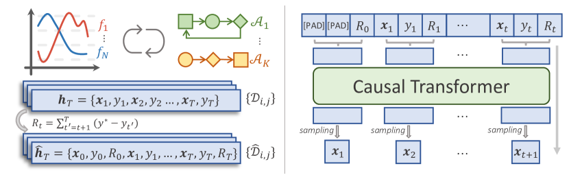
(a) Data Generation

(b) Training and Inference

Figure 1: Illustration of RIBBO. Left: Data Generation. $K$ existing BBO algorithms $\{\mathcal{A}_{j}\}_{j=1}^{K}$ and $N$ BBO tasks $\{f_{i}\}_{i=1}^{N}$ are used to serve as the behavior algorithms and the training tasks, respectively. The offline datasets $\{\mathcal{D}_{i,j}\}$ consist of the optimization histories $\bm{h}_{T}=\{(\bm{x}_{t},y_{t})\}_{t=1}^{T}$ collected by executing each behavior algorithm $\mathcal{A}_{j}$ on each task $f_{i}$ for $T$ evaluation steps, which are then augmented with the regret-to-go tokens $R_{t}$ (calculated as the cumulative regret $\sum^{T}_{t^{\prime}=t+1}(y^{*}-y_{t^{\prime}})$ over the future optimization history) to generate the final dataset $\{\widehat{\mathcal{D}}_{i,j}\}$ for training. Right: Training and Inference. Our model takes in triplets of $(\bm{x}_{t},y_{t},R_{t})$, embeds them into one token, and outputs the distribution over the next query point $\bm{x}_{t+1}$. During training, the ground-truth next query is used to minimize the loss in Eq. (4). During inference, the next query point $\bm{x}_{t+1}$ is generated auto-regressively based on the current history $\hat{\bm{h}}_{t}$.

3 Method

This section presents Reinforced In-context Black-Box Optimization (RIBBO), which learns an enhanced BBO algorithm in an E2E fashion. The overall workflow is presented in Figure 1.

3.1 Problem Formulation

We follow the task-distribution assumption, which is commonly adopted in meta-learning settings [19; 28; 64]. Our goal is to learn a generalizable model $\mathcal{M}$ capable of solving a wide range of BBO tasks, each associated with a BBO objective function $f$ sampled from the task distribution $P(\mathcal{F})$, where $\mathcal{F}$ denotes the function space.

Let $[N]$ denote the integer set $\{1,2,\ldots,N\}$. During training, we usually access $N$ source tasks and each task corresponds to an objective function $f_{i}\sim P(\mathcal{F})$, where $i\in[N]$. Hereafter, we use $f_{i}$ to denote the task $i$ if the context is clear. We assume that the information is available via offline datasets $\mathcal{D}_{i,j}$, which are produced by executing a behavior algorithm $\mathcal{A}_{j}$ on task $f_{i}$, where $j\in[K]$ and $i\in[N]$. Each dataset $\mathcal{D}_{i,j}=\{\bm{h}^{i,j,m}_{T}\}_{m=1}^{M}$ consists of $M$ optimization histories $\bm{h}^{i,j,m}_{T}=\{(\bm{x}_{t},y_{t})\}_{t=1}^{T}$, where $\bm{x}_{t}$ is the query point selected by $\mathcal{A}_{j}$ at iteration $t$, and $y_{t}=f_{i}(\bm{x}_{t})$ is its objective value. If the context is clear, we will omit $i,j,m$ and simply use $\bm{h}_{T}$ to denote an optimization history with length $T$. The initial history $\bm{h}_{0}$ is defined as $\emptyset$. We impose no additional assumptions about the behavior algorithms, allowing for a range of BBO algorithms, even random search.

With the datasets, we seek to learn a model $\mathcal{M}_{\bm{\theta}}(\bm{x}_{t}|\bm{h}_{t-1})$, which is parameterized by $\bm{\theta}$ and generates the next query point $\bm{x}_{t}$ by conditioning on the previous history $\bm{h}_{t-1}$. As introduced in Section 2.1, with a given budget $T$ and the history $\bm{h}_{T}$ produced by an algorithm $\mathcal{A}$, we use the cumulative regret

$${\rm Reg}_{T}=\sum_{t=1}\nolimits^{T}(y^{*}-y_{t})$$ (1)

as the evaluation metric, where $y^{*}$ is the optimum value and $\{y_{t}\}^{T}_{t=1}$ are the function values of the points in $\bm{h}_{T}$.

3.2 Method Outline

Given the current history $\bm{h}_{t-1}$ at iteration $t$, a BBO algorithm selects the next query point $\bm{x}_{t}$, observes the function value $y_{t}=f_{i}(\bm{x}_{t})$, and updates the history $\bm{h}_{t}=\bm{h}_{t-1}\cup\{(\bm{x}_{t},y_{t})\}$. Similar to the previous work [13], we take this framework as a starting point and define the learning of a universal BBO algorithm as learning a model $\mathcal{M}_{\bm{\theta}}$, which takes the preceding history $\bm{h}_{t-1}$ as input and outputs a distribution of the next query point $\bm{x}_{t}$. The optimization histories in offline datasets provide a natural supervision for learning.

Suppose we have a set of histories $\{\bm{h}_{T}\}$, generated by a single behavior algorithm $\mathcal{A}$ on a single task $f$. By employing a causal transformer model $\mathcal{M}_{\bm{\theta}}$, we expect $\mathcal{M}_{\bm{\theta}}$ to imitate $\mathcal{A}$ and produce similar optimization history on $f$. In practice, we usually have datasets containing histories from multiple behavior algorithms $\{\mathcal{A}_{j}\}_{j=1}^{K}$ on multiple tasks $\{f_{i}\}_{i=1}^{N}$. To fit $\mathcal{M}_{\bm{\theta}}$, we use the negative log-likelihood loss

$$\mathcal{L}_{\rm BC}(\bm{\theta})=-\mathbb{E}_{\bm{h}_{T}\sim\mathcal{D}_{i,j}}\left[\sum_{t=1}^{T}\log\mathcal{M}_{\bm{\theta}}(\bm{x}_{t}|\bm{h}_{t-1})\right].$$ (2)

To effectively minimize the loss, $\mathcal{M}_{\bm{\theta}}$ needs to recognize both the task and the behavior algorithm in-context, and then imitate the optimization behavior of the corresponding behavior algorithm.

Nevertheless, naively imitating the offline datasets hinders the model since some inferior behavior algorithms may severely degenerate the model’s performance. Inspired by DT [12], we propose to augment the optimization history with Regret-To-Go (RTG) tokens $R_{t}$, defined as the sum of instantaneous regrets over the future history:

$$\hat{\bm{h}}_{T}=\{(\bm{x}_{t},y_{t},R_{t})\}_{t=0}^{T},\;R_{t}=\sum_{t^{\prime}=t+1}^{T}(y^{*}-y_{t^{\prime}}),$$ (3)

where $\bm{x}_{0}$ and $y_{0}$ are placeholders for padding, denoted as [PAD] in Figure 1(b), and $R_{T}=0$. The augmented histories compose the augmented dataset $\widehat{\mathcal{D}}_{i,j}$, and the training objective of $\mathcal{M}_{\bm{\theta}}$ becomes

$$\mathcal{L}_{\rm{RIBBO}}(\bm{\theta})=-\mathbb{E}_{\hat{\bm{h}}_{T}\sim\widehat{\mathcal{D}}_{i,j}}\left[\sum_{t=1}^{T}\log\mathcal{M}_{\bm{\theta}}(\bm{x}_{t}|\hat{\bm{h}}_{t-1})\right].$$ (4)

The integration of RTG tokens offers several advantages. 1) RTG tokens in the context bring identifiability of behavior algorithms, and the model $\mathcal{M}_{\bm{\theta}}$ can effectively utilize them to make appropriate decisions. 2) RTG tokens have a direct correlation with the metric of interest, i.e., cumulative regret $\mathrm{Reg}_{T}$ in Eq. (1). Conditioning on a lower RTG token provides a guidance to our model and reinforces $\mathcal{M}_{\bm{\theta}}$ to exhibit superior performance. These advantages will be clearly shown by experiments in Section 4.4.

Note that the resulting method RIBBO has implicitly utilized the in-context learning capacity of transformer to guide the optimization with previous histories and the desired future regret as context. The in-context learning capacity of inferring the tasks at hand based on the input contexts has been observed as the scale of data and model increases [31]. It has been explored to infer general functional relationships as supervised learning or RL algorithms. For example, Guo et al. [25]; Hollmann et al. [27]; Li et al. [37] feed the training dataset $\{(\bm{x}_{i},y_{i})\}_{i=1}^{t-1}$ as the context and expect the model to make an accurate prediction on the query input $\bm{x}_{t}$; Laskin et al. [35] learn RL algorithms using causal transformers. Here, we use it for BBO.

3.3 Practical Implementation

Next, we detail the model architecture, training and inference of RIBBO.

Model Architecture. For the formalization of the model $\mathcal{M}_{\bm{\theta}}$, we adopt the commonly used GPT architecture [47], which comprises a stack of causal attention blocks, each containing an attention component and a feed-forward network. We aggregate each triplet $(\bm{x}_{i},y_{i},R_{i})$ using a two-layer MLP network. The output of $\mathcal{M}_{\bm{\theta}}$ is a diagonal Gaussian distribution of the next query point.

Note that previous works that adopt the sequence model as the surrogate model [42; 39; 40] typically remove the positional encoding because the surrogate model should be invariant to the history order. On the contrary, our implementation preserves the positional encoding, naturally following the behavior of certain algorithms (e.g., BO or EA) and making it easier to learn from algorithms. Additionally, the positional encoding can keep the monotonically decreasing order of RTG tokens. More architecture details can be found in Appendix A.

Model Training. RTG tokens are computed as outlined in Eq. (3) for the offline datasets before training. As the calculation of regret requires the optimum value of task $i$, we use the best-observed value $y_{\rm max}^{i}$ as a proxy for the optimum value. Let $\{\widehat{\mathcal{D}}_{i,j}\}_{i\in[N],j\in[K]}$ denote the RTG augmented datasets with $N$ tasks and $K$ algorithms. We sample a minibatch of consecutive subsequences of length $\tau<T$ uniformly from the augmented datasets and train $\mathcal{M}_{\bm{\theta}}$ to minimize the RIBBO loss in Eq. (4).

Algorithm 1 Model Inference with HRR

Input: trained model $\mathcal{M}_{\bm{\theta}}$, budget $T$, optimum value $y^{*}$
Process:

1:  Initialize context $\hat{\bm{h}}_{0}=\{(\bm{x}_{0},y_{0},R_{0})\}$, where $\bm{x}_{0}$ and $y_{0}$ are placeholders for padding and $R_{0}=0$;

2:  for $t=1,2,\ldots,T$ do

3:     Generate the next query point $\bm{x}_{t}\sim\mathcal{M}_{\bm{\theta}}(\bm{\cdot}|\hat{\bm{h}}_{t-1})$;

4:     Evaluate $\bm{x}_{t}$ to obtain $y_{t}=f(\bm{x}_{t})$;

5:     Calculate the instantaneous regret $r=y^{*}-y_{t}$;

6:     Relabel $R_{i}\leftarrow R_{i}+r$, for each $(\bm{x}_{i},y_{i},R_{i})$ in $\hat{\bm{h}}_{t-1}$;

7:     $\hat{\bm{h}}_{t}=\hat{\bm{h}}_{t-1}\cup\{(\bm{x}_{t},y_{t},0)\}$;

8:  end for

Model Inference. The model $\mathcal{M}_{\bm{\theta}}$ generates the query points $\bm{x}_{t}$ auto-regressively during the inference process, which involves iteratively selecting a new query point $\bm{x}_{t}$ based on the current augmented history $\hat{\bm{h}}_{t-1}$, evaluating the query as $y_{t}=f(\bm{x}_{t})$, and updating the history $\hat{\bm{h}}_{t}=\hat{\bm{h}}_{t-1}\cup\{(\bm{x}_{t},y_{t},R_{t})\}$. A critical aspect of this process is how to specify the value of RTG (i.e., $R_{t}$) at every iteration $t$. Inspired by DT, a naive approach is to specify a desired performance as the initial RTG $R_{0}$, and then decrease it as

$$R_{t}=R_{t-1}-(y^{*}-y_{t}).$$ (5)

However, this strategy has the risk of producing out-of-distribution RTGs, since the values can fall below $0$ due to an improperly selected $R_{0}$.

Given the fact that RTGs are lower bounded by $0$ and a $0$ value implies a good BBO algorithm with low regret, we propose to set the immediate RTG as 0, and use a strategy called Hindsight Regret Relabelling (HRR) to update previous RTGs based on the current sampling. The inference procedure with HRR is detailed in Algorithm 1. In line 1, the history $\hat{\bm{h}}_{0}$ is initialized with padding placeholders $\bm{x}_{0},y_{0}$ and RTG $R_{0}=0$. At iteration $t$ (i.e., lines 3–7), the model $\mathcal{M}_{\bm{\theta}}$ is first fed with the augmented history $\hat{\bm{h}}_{t-1}$ to generate the next query point $\bm{x}_{t}$ in line 3, and $\bm{x}_{t}$ is evaluated to obtain $y_{t}=f(\bm{x}_{t})$ in line 4. Then, the immediate RTG $R_{t}$ is set to $0$, and we employ HRR to update RTG tokens in the history $\hat{\bm{h}}_{t-1}$: calculating the instantaneous regret $r=y^{*}-y_{t}$ in line 5 and adding $r$ to every RTG token in $\hat{\bm{h}}_{t-1}$ in line 6, i.e.,

$$\forall 0\leq i<t,R_{i}\leftarrow R_{i}+(y^{*}-y_{t}).$$ (6)

Note that this relabelling process guarantees that $\forall 0\leq i<t$, the RTG token $R_{i}=\sum_{t^{\prime}=i+1}^{t}(y^{*}-y_{t^{\prime}})$, which can also be written as $\sum_{t^{\prime}=i+1}^{T}(y^{*}-y_{t^{\prime}})$, consistent with the definition in Eq. (3), because the immediate RTG $R_{t}=\sum_{t^{\prime}=t+1}^{T}(y^{*}-y_{t^{\prime}})$ is set to 0. In line 7, the history $\hat{\bm{h}}_{t}$ is updated by expanding $\hat{\bm{h}}_{t-1}$ with $\{(\bm{x}_{t},y_{t},0)\}$, i.e., the current sampling and its immediate RTG $R_{t}=0$. The above process is repeated until reaching the budget $T$. Thus, we can find that HRR not only exploits the full potential of $\mathcal{M}_{\bm{\theta}}$ through using zero as the immediate RTG and thereby demands the model to generate the most advantageous decisions, but also preserves the calculation of RTG tokens following the same way as the training data, i.e., representing the cumulative regret over the future optimization history.

3.4 Data Generation

Finally, we give some guidelines about data generation for using the proposed RIBBO method.

Data Collection. Given a set of tasks $\{f_{i}\}_{i=1}^{N}$ sampled from the task distribution $P(\mathcal{F})$, we can select a diverse set of algorithms for data collection. For example, we can select some representatives of different types of BBO algorithms (e.g., BO and EA). Datasets $\mathcal{D}_{i,j}$ are then obtained by using each behavior algorithm to optimize each function with different random seeds. Each optimization history $\bm{h}_{T}=\{(\bm{x}_{t},y_{t})\}_{t=1}^{T}$ in $\mathcal{D}_{i,j}$ is then augmented using RTG tokens $R_{t}$ computed as in Eq. (3). The resulting augmented histories $\hat{\bm{h}}_{T}=\{(\bm{x}_{t},y_{t},R_{t})\}_{t=0}^{T}$ compose the final datasets $\widehat{\mathcal{D}}_{i,j}$ for training the model $\mathcal{M}_{\bm{\theta}}$.

Data Normalization. To provide a unified interface and balance the statistic scales across tasks, it is important to apply normalization to the inputs to our model. We normalize the point $\bm{x}$ by $(\bm{x}-\bm{x}_{\rm min})/(\bm{x}_{\rm max}-\bm{x}_{\rm min})$, with $\bm{x}_{\rm max}$ and $\bm{x}_{\rm min}$ being the upper and lower bounds of the search space, respectively. For the function value $y$, we apply random scaling akin to previous works [61; 14]. That is, when sampling a history $\bm{h}_{\tau}$ from the datasets $\mathcal{D}_{i,j}$, we randomly sample the lower bound $l\sim\mathcal{U}(y^{i}_{\rm min}-\frac{s}{2},y^{i}_{\rm min}+\frac{s}{2})$ and the upper bound $u\sim\mathcal{U}(y^{i}_{\rm max}-\frac{s}{2},y^{i}_{\rm max}+\frac{s}{2})$, where $\mathcal{U}$ stands for uniform distribution, $y^{i}_{\rm min},y^{i}_{\rm max}$ denote the observed minimum and maximum values for $f_{i}$, and $s=y^{i}_{\rm max}-y^{i}_{\rm min}$; the values $y_{t}$ in $\bm{h}_{\tau}$ are then normalized by $(y_{t}-l)/(u-l)$. The RTG tokens are calculated accordingly with the normalized values. The random normalization can make a model exhibit invariance across various scales of $y$.

4 Experiments

In this section, we examine the performance of RIBBO on a wide range of tasks, including synthetic functions, Hyper-Parameter Optimization (HPO) and robot control problems. The model architecture and hyper-parameters are maintained consistently across these problems. We train our model using five distinct random seeds, ranging from $0$ through $4$, and each trained model is also run five times independently during the execution phase. We will report the average performance and standard deviation. Details of the model hyper-parameters can be found in Appendix A. Our code is available at https://github.com/songlei00/RIBBO.

4.1 Experimental Setup

Benchmarks. We use BBO Benchmarks BBOB [15], HPO-B [2], and rover trajectory planning tasks [57]. The BBOB suite, a comprehensive and widely used benchmark in the continuous domain, consists of $24$ synthetic functions. For each function, a series of transformations are implemented on the search space to obtain a distribution of functions with similar properties. According to the properties of the functions, they can be further divided into $5$ categories, and we select one from each category due to resource constraints, including Greiwank Rosenbrock, Lunacek, Rastrigin, Rosenbrock, and Sharp Ridge. HPO-B is the most commonly used HPO benchmark and consists of a series of HPO problems. It fits an XGBoost model as the objective function for each HPO problem, and we conduct experiments on two widely used machine models, SVM and XGBoost. For robot control optimization, we perform experiments on rover trajectory planning, which is a trajectory optimization task to emulate rover navigation. Similar to [15; 56], we implement random translations and scalings to the search space to construct a distribution of functions. For BBOB and rover problems, we sample a set of functions as training and test tasks, while for HPO-B, we use the meta-training/test splits provided by the authors. Detailed explanations of the benchmarks can be found in Appendix B.1.

Data. Similar to OptFormer [14], we employ seven behavior algorithms, i.e., Random Search, Shuffled Grid Search, Hill Climbing, Regularized Evolution [49], Eagle Strategy [63], CMA-ES [26], and GP-EI [8], which are representatives of heuristic search, EA, and BO, respectively. Datasets are generated by using each behavior algorithm to optimize each training function with different random seeds. More details about the behavior algorithms and datasets can be found in Appendix B.2 and B.3.

4.2 Baselines

As our proposed method RIBBO is an in-context E2E model, the most related baselines are those also training an E2E model with an offline dataset, including Behavior Cloning (BC) [7] and OptFormer [14]. Their hyper-parameters are set as same as that of our model for fairness. Note that the seven behavior algorithms used to generate datasets are also important baselines, which are included for comparison as well.

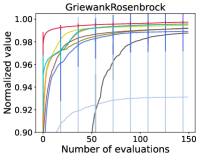
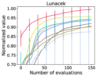
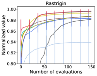
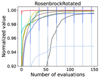
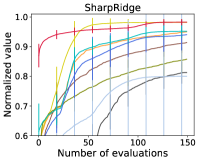
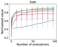
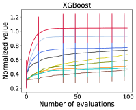
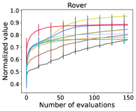
Figure 2: Performance comparison among RIBBO, BC, BC Filter, OptFormer, and behavior algorithms on synthetic functions, HPO, and robot control problems. The $y$-axis is the normalized average objective value, and the length of vertical bars represents the standard deviation.

BC uses the same transformer architecture as RIBBO. The only difference is that we do not feed RTG tokens into the model of BC and train to minimize the BC loss in Eq. (2). When the solutions are generated auto-regressively, BC tends to imitate the average behavior of various behavior algorithms. Consequently, the inclusion of underperforming algorithms, e.g., Random Search and Shuffled Grid Search, may significantly degrade the performance. To mitigate this issue, we have also trained the model by excluding these underperforming algorithms, denoted as BC Filter.

OptFormer employs transformer to imitate the behaviors of a set of algorithms and needs to manually specify the imitated algorithm during execution. Its original implementation is built upon a text-based transformer with a large training scale. In this paper, we re-implemented a simplified version of OptFormer where we only maintain the algorithm type within the metadata, i.e., employing different initial states $\bm{x}_{0}$ and $y_{0}$ for different algorithms. More details about the training procedure and imitation capacity of the reimplementation can be found in Appendix C.

4.3 Main Results

The results are shown in Figure 2. For the sake of clarity in visualization, we have omitted the inclusion of Random Search and Shuffled Grid Search due to their poor performance from start to finish. We can observe that RIBBO achieves superior or at least equivalent efficacy in comparison to the best behavior algorithm on each problem except SVM and rover. This demonstrates the versatility of RIBBO, while the most effective behavior algorithm depends upon the specific problem at hand, e.g., the best behavior algorithms on Lunacek, Rastrigin and XGBoost are GP-EI, Eagle Strategy and CMA-ES, respectively. Note that the good performance of RIBBO does not owe to the memorization of optimal solutions, as the search space is transformed randomly, resulting in variations in optimal solutions across different functions from the same distribution. It is because RIBBO is capable of using RTG tokens to identify algorithms and reinforce the performance on top of the behavior algorithms, which will be clearly shown later. We can also observe that RIBBO performs extremely well in the early stage, which draws the advantage from the HRR strategy, i.e., employing zero as the immediate RTG to generate the optimal potential solutions.

RIBBO does not perform well on SVM problem, which may be due to the problem’s low-dimensional nature (only three parameters) and its relative simplicity for optimization. Behavior algorithms can easily achieve good performance, while the complexity of RIBBO’s training and inference processes could instead result in the performance degradation. Regarding to rover problem where GP-EI performs the best, we collect less data from GP-EI than other behavior algorithms due to the high time cost. This may limit RIBBO’s capacity to leverage the high-quality data from GP-EI, given its small proportion relative to the data collected from other behavior algorithms. Despite this, RIBBO is still the runner-up, significantly surpassing the other behavior algorithms.

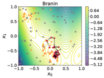
(a) Visualization

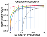
(b) Cross-dist generalization

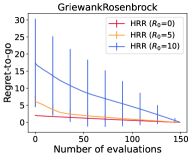
(c) Initial RTGs

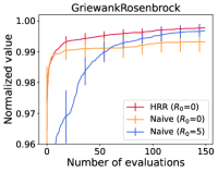
(d) RTG update strategy

Figure 3: (a) Visualization of the contour lines of 2D Branin function and sampling points of RIBBO (red), Eagle Strategy (orange), and Random Search (gray), where the arrows represent the optimization trajectory of RIBBO. (b) Cross-distribution generalization by training the model on $4$ synthetic functions and testing on the remaining one, GriewankRosenbrock, which has different properties. Note that the legend shares with that of Figure 2. (c) Initial RTG $R_{0}$’s influence on performance. (d) RTG update strategy comparison between HRR and the naive strategy with different $R_{0}$.

Compared with BC and BC Filter, RIBBO performs consistently better except on the SVM problem. BC tends to imitate the average behavior of various algorithms, and its poor performance is due to the aggregation of data from behavior algorithms with inferior performance. BC Filter is generally better than BC, because the data from the two underperforming behavior algorithms, i.e., Random Search and Shuffled Grid Search, are manually excluded for the training of BC Filter. As introduced before, OptFormer requires to manually specify which algorithm to execute. We have specified the behavior algorithm Eagle Strategy in Figure 2, which obtains good overall performance on these problems. It can be observed that OptFormer displays a close performance to Eagle Strategy, while RIBBO performs better. More results about the imitation capacity of OptFormer can be found in Appendix C.

Why Does RIBBO Behave Well? To better understand RIBBO, we train the model using only two behavior algorithms, Eagle Strategy and Random Search, which represent a good algorithm and an underperforming one, respectively. Figure 3(a) visualizes the contour lines of the 2D Branin function and the sampling points of RIBBO, Eagle Strategy, and Random Search, represented by red, orange, and gray points, respectively. The arrows are used to represent the optimization trajectory of RIBBO. Note that the two parameters of Branin have been scaled to $[-1,1]$ for better visualization. It can be observed that RIBBO makes a prediction preferring Eagle Strategy over Random Search, indicating its capability to automatically identify the quality of training data. Additionally, RIBBO achieves the exploration and exploitation trade-off capability using its knowledge about the task obtained during training, thus generating superior solutions over the ones in the training dataset.

Cross-Distribution Generalization. We further conduct experiments to examine the generalization of RIBBO to unseen function distributions. For this purpose, we train the model on $4$ of the $5$ chosen synthetic functions and test it with the remaining one. Note that each function (i.e., Greiwank Rosenbrock, Lunacek, Rastrigin, Rosenbrock, and Sharp Ridge) here actually represents a distribution of functions with similar properties, and we sample a set of functions from each distribution as introduced before. Greiwank Rosenbrock is used for testing. The results in Figure 3(b) suggest that RIBBO has a strong generalizing ability to unseen function distributions. More results on cross-distribution generalization are deferred to Appendix D.

The good generalization of RIBBO can be attributed to the paradigm of learning the entire algorithm, which can acquire general knowledge, such as exploration and exploitation trade-off from data, as observed in [13]. In contrast, such generalization may be limited if we learn surrogate models from data, because the function landscape inherent to surrogate models will contain only the knowledge of similar functions.

4.4 Ablation Studies

RIBBO augments the histories with RTG tokens, facilitating distinguishing algorithms and automatically generating algorithms with user-specified performance. Next, we will verify the effectiveness of RTG conditioning and HRR strategy.

Influence of Initial RTG Token $R_{0}$. By incorporating RTG tokens into modeling, RIBBO should be able to attend to the RTGs and generate optimization trajectories that achieve the specified initial RTG token $R_{0}$. To validate this, we examine the performance of RIBBO when specifying different values of $R_{0}$, and the results are presented in Figure 3(c). Here, the RTG values, instead of the normalized objective values, of the trajectory are used as the $y$-axis. We can observe that the cumulated regrets of the generated query sequence do correlate with the specified RTG, indicating that RIBBO establishes the connection between regret and generation.

Effectiveness of HRR. A key point of the inference procedure is how to update the value of RTG tokens at each iteration. To assess the effectiveness of the proposed strategy HRR in Eq. (6), we compare it with the naive strategy in Eq. (5), which sets an initial RTG token $R_{0}$ and decreases it by the one-step regret after each iteration. The results are shown in Figure 3(d). The naive strategy displays distinct behaviors when $R_{0}=0$ or $R_{0}=5$. When $R_{0}=0$ i.e. the lower bound of regret, the model performs well in the initial stage. However, as the optimization progresses, the RTG tokens gradually decrease to negative values, leading to poor performance since negative RTGs are out-of-distribution values. Using $R_{0}=5$ compromises the initial performance, as the model may not choose the most aggressive solutions with a high $R_{0}$. However, higher $R_{0}$ yields better convergence value since it prevents out-of-distribution RTGs in the late stage. The proposed HRR strategy performs the best across the whole optimization stage, because setting the immediate RTG as $0$ encourages the model to make the most advantageous decisions at every iteration, while hindsight relabeling of previous RTG tokens in Eq. (6) keeps the values meaningful and feasible.

Other Ablation Studies. We also study the effect of the method to aggregate $(\bm{x}_{i},y_{i},R_{i})$ tokens, the normalization method for the function value $y$, the model size, and the length $\tau$ of sampled subsequences. Due to space limitation, we provide the results in Appendix E.

5 Conclusion

This paper proposes RIBBO, which employs a transformer architecture to learn a reinforced BBO algorithm from offline datasets in an E2E fashion. By incorporating RTG tokens into the optimization histories, RIBBO can automatically generate optimization trajectories satisfying the user-desired regret. Comprehensive experiments on BBOB, HPO and robot control problems show the versatility of RIBBO. This work is a preliminary attempt towards universal BBO, and we hope it can encourage more explorations in this direction. For example, we only consider the model training over continuous search space with the same dimensionality, and it would be interesting to explore heteroscedastic search space with different types of variables.

Potential Broader Impact

This paper presents work whose goal is to advance the field of black-box optimization. There are many potential societal consequences of our work, none of which we feel must be specifically highlighted here.

Appendix A Model Details

We employ the commonly used GPT architecture [47] and the hyper-parameters are maintained consistently across the problems. Details can be found in Table 1. For BC, BC Filter and OptFormer, the hyper-parameters are set as same as that of our model.

Table 1: List of hyper-parameter settings in RIBBO.

RIBBO
Embedding dimension	256
Number of self-attention layers	12
Number of self-attention heads	8
Point-wise feed-forward dimension	1024
Dropout rate	0.1
Batch size	64
Learning rate	0.0002
Learning rate decay	0.01
Optimizer	Adam
Optimizer scheduler	Linear warm up and cosine annealing
Number of training steps	500,000
Length of subsequence $\tau$	50

Appendix B Details of Experimental Setup

B.1 Benchmarks

• BBOB [15] is a widely used synthetic BBO benchmark, consisting of $24$ synthetic functions in continue domain. This benchmark makes a series of transformations in the search space, such as linear transformations (e.g., translation, rotation, scaling) and non-linear transformations (e.g., Tosz, Tasy), to create a distribution of functions while retaining similar properties. According to the properties of functions, these synthetic functions can be divided into $5$ categories, i.e., (1) separable functions, (2) moderately conditioned functions, (3) ill-conditioned and unimodal functions, (4) multi-modal functions with adequate global structure, and (5) multi-modal functions with weak global structures. We select one function from each category to evaluate our algorithm, Rastrigin from (1), Rosenbrock Rotated from (2), Sharp Ridge from (3), Greiwank Rosenbrock from (4), and Lunacek from (5). We use the BBOB benchmark implementation in Open Source Vizier. The dimension is set to $10$ for all functions.

• SVM and XGBoost. HPO-B [2] is the most commonly used HPO benchmark and grouped by search space id. Each search space id corresponds to a machine learning model, e.g., SVM or XGBoost. Each such search space has multiple associated dataset id, which is a particular HPO problem, i.e., optimizing the performance of the corresponding model on a dataset. For continue domain, it fits an XGBoost model as the objective function for each HPO problem. These datasets for each search space id are divided into training and test datasets. We examine our method on two selected search space id, i.e., $5527$ and $6767$, which are two representative HPO problems tuning SVM and XGBoost, respectively. SVM has $3$ parameters, while XGBoost has $18$ parameters, which is the most parameters in HPO-B.

• Rover Trajectory Planning [57; 16] is a trajectory optimization task to emulate a rover navigation task. The trajectory is determined by fitting a B-spline to $30$ points in a $2$D plane, totally $60$ parameters to optimize. Given $\bm{x}\in[0,1]^{60}$, the objective function is $f(\bm{x})=c(\bm{x})+\lambda(\|\bm{x}_{0,1}-\bm{x}_{s}\|_{1}+\|\bm{x}_{58,59}-\bm{x}_{g}\|_{1})+b$, where $c(\bm{x})$ is the cost of a given trajectory, $\bm{x}_{s}$ and $\bm{x}_{g}$ are $2$D points that specify the starting and goal positions in the plane, $\lambda$ and $b$ are parameters to define the problem. This problem is non-smooth, discontinuous, and concave over the first two and last two dimensions. To construct the distribution of functions, we applied translations in $[-0.1,0.1]^{d}$ as well as scalings in $[0.9,1.1]$, similar to [56; 15]. The training and test tasks are randomly sampled from the distribution.

B.2 Bahavior Algorithms

The datasets are generated with some representatives of heuristic search, EA, and BO as behavior algorithms. We use the implementation in Open Source Vizier [51] for Random Search, Shuffled Grid Search, Eagle Strategy, CMA-ES. For Hill Climbing and Regularized Evolution, we provide a simple reimplementation. We use the implementation in BoTorch [8] for GP-EI. The details of behavior algorithms are summarized as follows.

• Random Search uniformly at random selects a point in the domain at each iteration.

• Shuffled Grid Search discretizes the ranges of real parameters into $100$ equidistant points and then selects without replacement a random point from the grid at each iteration.

• Hill Climbing. At each iteration $t$, the current best solution $x_{best}$ is mutated (using the same mutation operation as Regularized Evolution) to $x_{next}$ and evaluated. If $f(x_{next})\textgreater f(x_{best})$, we update $x_{best}$ to $x_{next}$.

• Regularized Evolution [49] is an evolutionary algorithm with tournament selection and age-based replacement. We use a population size of $25$ and tournament size of $5$. At each iteration, we randomly select a tournament subset from the current population, and mutate the solution with maximum value. The mutation operation is to uniformly at random selects one of the parameters and mutates to a random value in the domain.

• Eagle Strategy [63] without the Levy random walk, aka Firefly Algorithm, maintains a population of fireflies. Each firefly emits a light whose intensity corresponds to the objective value. At each iteration, for a firefly, a weight is calculated to chase after a brighter firefly and actively move away from darker one in its vicinity, and the position is updated using the calculated weight.

• CMA-ES [26] is a popular evolutionary algorithm. At each iteration, the candidate solutions are sampled from a multivariate normal distribution and evaluated, then the mean and covariance matrix are updated.

• GP-EI employs GP as the surrogate model and EI [30] as the acquisition function for BO.

B.3 Data

For training, a set of tasks are sampled from the task distribution and above behavior algorithms are used to collect data. Specifically, for BBOB suite, a total of $200$ functions are sampled, and each behavior algorithm is executed $500$ times except GP-EI, which is limited to $100$ function samples due to high time cost. For HPO-B, we use the “v3” meta-training/test splits, which consist of $51$ training and $6$ test tasks for SVM, and similarly, $52$ training and $6$ test tasks for XGBoost. All behavior algorithms employ $500$ random seeds in the execution except GP-EI, which is executed using $500$ random seeds. For rover problem, $300$ functions are sampled with each being run $500$ times, whereas for GP-EI, a smaller number of $50$ functions is selected, each being run $500$ times. For testing, we randomly sample $10$ functions for each problem and run each algorithm multiple times to report the average performance and standard deviation.

Appendix C Re-Implementation of OptFormer

OptFormer [14] is a general optimization framework based on transformer [54] and provides an interface to learn policy or function prediction. When provided with textual representations of historical data, OptFormer is capable of determining the next query point $\bm{x}_{t}$ as policy. Additionally, if the histories incorporate a possible query point $\bm{x}_{t}$, the framework is designed to predict the corresponding $y_{t}$, thereby serving as function prediction. We concentrate on the aspect of policy learning, attributable to its greater relevance to our work.

The original implementation is built upon text-based transformer and uses private datasets for training. In this paper, we have re-implemented a simplified version of OptFormer, where we omit the textual tokenization process and only maintain the algorithm type within the metadata. Numerical inputs are fed into the model and we employ different initial states $\bm{x}_{0}$ and $y_{0}$ to represent different algorithms. The hyper-parameters are set as same as our method.

To examine the algorithm imitation capability, we compare our re-implemented with the corresponding behavior algorithms. The results are shown in Figure 4. For the sake of clarity in the visual representation, we only plot a subset of behavior algorithms, including Shuffled Grid Search, Hill Climbing, Regularized Evolution and Eagle Strategy. These behavior algorithms are plotted by solid lines, while their OptFormer counterparts are shown by dashed lines with the same color. Note that the figure is shown using the immediate function values as the $y$-axis to facilitate a comprehensive observation of the optimization.

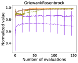
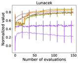
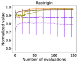
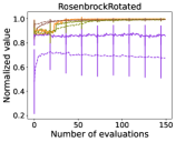
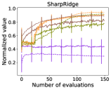
Figure 4: Comparison of the behavior algorithms with the OptFormer re-implementation.

Appendix D Cross-Distribution Generalization

We conduct experiments to examine the generalization of our method to unseen function distributions. We train the model on $4$ of $5$ chosen synthetic functions and test it with the remaining one. The results in Figure 5 have shown that RIBBO has a strong generalization ability to unseen function distributions.

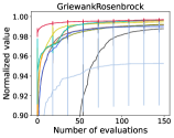
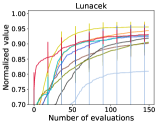
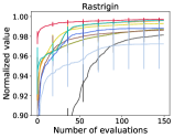
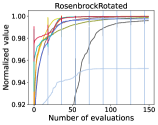
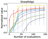
Figure 5: Cross-Distribution Generalization by training on $4$ synthetic functions and testing on the remaining one.

Appendix E Ablation Studies

We provide further ablation studies to examine the influence of the important components and hyper-parameters of RIBBO, including the method to aggregate $(\bm{x}_{i},y_{i},R_{i})$ tokens, the normalization method for the function value $y$, the model size, and the sampled subsequence length $\tau$ during training.

Token Aggregation aims to aggregate the information of $(\bm{x}_{i},y_{i},R_{i})$ tokens and establish associations between them. RIBBO employs the Concatenation method (Concat), i.e., concatenating to aggregate $\bm{x}_{i}$, $y_{i}$ and $R_{i}$ to form a single token. It is compared with two different token aggregation methods, i.e., Addition (Add) and Interleaving (Interleave). The addition method integrates the values of each token to form a single token, while interleaving method addresses each token sequentially. The results are shown in Figure 6(a). Concatenation method surpasses both the addition and interleaving methods, with the addition method exhibiting the least efficacy. The concatenation method employs a relatively straightforward technique to aggregate each token by direct concatenation, while the interleaving method adopts a more complex process to learn the interrelations of tokens. The inferior performance of the addition method is because that the summation will omit some details of the original tokens, which are necessary for the generation of the next query $\bm{x}_{t}$.

Normalization Method is to balance the scales of function value $y$ across tasks. We compare the employed random normalization with the dataset normalization and no normalization. Dataset normalization scales the value $y$ by $(y-y_{\rm min}^{i})/(y_{\rm max}^{i}-y_{\rm min}^{i})$ for task $i$, where $y_{\rm min}^{i}$ and $y_{\rm max}^{i}$ denote the observed minimum and maximum values for $f_{i}$, while no normalization entails utilizing the original function values. The results are shown in Figure 6(b). Random normalization and dataset normalization have similar performance, while no normalization leads to the poor performance. The normalization method has a direct effect on the calculation of RTG tokens and thereby influences the generating with a desired regret. No normalization results in significant variances in the scale of $y$, posing a challenge for the generation process. Both random and dataset normalization scale the value of $y$ within a reasonable range, thus facilitating the training and inference. Nevertheless, random normalization can make a model exhibit invariance across various scales of $y$ as mentioned in [61; 14]. Consequently, we recommend to use random normalization in practice.

Model Size has an effect on the in-context learning ability. We compare the performance of the employed model size with a smaller one (8 layers, 4 attention heads and 128-dimensional embedding space) and a larger one (16 layers, 12 attention heads and 384-dimensional embedding space). The results are shown in Figure 6(c), indicating that the model’s size has small impact on its overall performance. A smaller model, with limited capacity, exhibits a diminished capability to the in-context learning ability, while a larger model requires more training data, potentially leading to a slight decrement in performance.

Subsequence Length $\tau$ controls the length of context during both training and inference phases. Employing subsequence sampling can be viewed as a form of data augmentation that facilitates the training process. As shown in Figure 6(d), sampling subsequences instead of using the entire history as context, specifically when $\tau=T=150$, leads to an improvement of the performance. Causal transformer training and inference are quadratic in the context length, hence, a smaller $\tau$ can result in reduced computational complexity. However, an excessively shortened context may contain insufficient historical information, which could, in turn, adversely affect the performance.

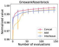
(a) Token aggregation

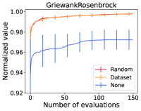
(b) Normalization method

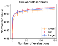
(c) Model size

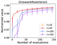
(d) Subsequence length $\tau$

Figure 6: Ablation studies of token aggregation, normalization method, model size, and the subsequence length $\tau$.

References

- Alarie et al. [2021] Alarie, S., Audet, C., Gheribi, A. E., Kokkolaras, M., and Le Digabel, S. Two decades of blackbox optimization applications. EURO Journal on Computational Optimization, 9:100011, 2021.
- Arango et al. [2021] Arango, S. P., Jomaa, H. S., Wistuba, M., and Grabocka, J. HPO-B: A large-scale reproducible benchmark for black-box HPO based on OpenML. arXiv preprint arXiv:2106.06257, 2021.
- Astudillo & Frazier [2021] Astudillo, R. and Frazier, P. I. Thinking inside the box: A tutorial on grey-box Bayesian optimization. In Proceedings of the 51st Winter Simulation Conference (WSC’21), pp. 1–15, Phoenix, AZ, 2021.
- Audet & Hare [2017] Audet, C. and Hare, W. Derivative-Free and Blackbox Optimization. Springer, 2017.
- Back [1996] Back, T. Evolutionary Algorithms in Theory and Practice: Evolution Strategies, Evolutionary Programming, Genetic Algorithms. Oxford University Press, 1996.
- Bai et al. [2023] Bai, T., Li, Y., Shen, Y., Zhang, X., Zhang, W., and Cui, B. Transfer learning for Bayesian optimization: A survey. arXiv preprint arXiv:2302.05927, 2023.
- Bain & Sammut [1995] Bain, M. and Sammut, C. A framework for behavioural cloning. Machine Intelligence, 15:103–129, 1995.
- Balandat et al. [2020] Balandat, M., Karrer, B., Jiang, D. R., Daulton, S., Letham, B., Wilson, A. G., and Bakshy, E. BoTorch: A framework for efficient Monte-Carlo Bayesian optimization. In Advances in Neural Information Processing Systems 33 (NeurIPS’20), pp. 10113–10124, Virtual, 2020.
- Brown et al. [2020] Brown, T. B., Mann, B., Ryder, N., Subbiah, M., Kaplan, J., Dhariwal, P., Neelakantan, A., Shyam, P., Sastry, G., Askell, A., Agarwal, S., Herbert-Voss, A., Krueger, G., Henighan, T., Child, R., Ramesh, A., Ziegler, D. M., Wu, J., Winter, C., Hesse, C., Chen, M., Sigler, E., Litwin, M., Gray, S., Chess, B., Clark, J., Berner, C., McCandlish, S., Radford, A., Sutskever, I., and Amodei, D. Language models are few-shot learners. In Advances in Neural Information Processing Systems 33 (NeurIPS’20), pp. 1877–1901, Virtual, 2020.
- Calandra et al. [2016] Calandra, R., Seyfarth, A., Peters, J., and Deisenroth, M. P. Bayesian optimization for learning gaits under uncertainty - An experimental comparison on a dynamic bipedal walker. Annals of Mathematics and Artificial Intelligence, 76(1-2):5–23, 2016.
- Chatzilygeroudis et al. [2019] Chatzilygeroudis, K., Vassiliades, V., Stulp, F., Calinon, S., and Mouret, J.-B. A survey on policy search algorithms for learning robot controllers in a handful of trials. IEEE Transactions on Robotics, 36(2):328–347, 2019.
- Chen et al. [2021] Chen, L., Lu, K., Rajeswaran, A., Lee, K., Grover, A., Laskin, M., Abbeel, P., Srinivas, A., and Mordatch, I. Decision transformer: Reinforcement learning via sequence modeling. In Advances in Neural Information Processing Systems 34 (NeurIPS’21), pp. 15084–15097, Virtual, 2021.
- Chen et al. [2017] Chen, Y., Hoffman, M. W., Colmenarejo, S. G., Denil, M., Lillicrap, T. P., Botvinick, M., and Freitas, N. Learning to learn without gradient descent by gradient descent. In Proceedings of the 34th International Conference on Machine Learning (ICML’17), pp. 748–756, Sydney, Australia, 2017.
- Chen et al. [2022] Chen, Y., Song, X., Lee, C., Wang, Z., Zhang, R., Dohan, D., Kawakami, K., Kochanski, G., Doucet, A., Ranzato, M., Perel, S., and de Freitas, N. Towards learning universal hyperparameter optimizers with transformers. In Advances in Neural Information Processing Systems 35 (NeurIPS’22), pp. 32053–32068, New Orleans, LA, 2022.
- Elhara et al. [2019] Elhara, O., Varelas, K., Nguyen, D., Tusar, T., Brockhoff, D., Hansen, N., and Auger, A. COCO: The large scale black-box optimization benchmarking (BBOB-largescale) test suite. arXiv preprint arXiv:1903.06396, 2019.
- Eriksson et al. [2019] Eriksson, D., Pearce, M., Gardner, J. R., Turner, R., and Poloczek, M. Scalable global optimization via local Bayesian optimization. In Advances in Neural Information Processing Systems 32 (NeurIPS’19), pp. 5497–5508, Vancouver, Canada, 2019.
- Feurer et al. [2015] Feurer, M., Springenberg, J., and Hutter, F. Initializing Bayesian hyperparameter optimization via meta-learning. In Proceedings of the 29th AAAI Conference on Artificial Intelligence (AAAI’15), pp. 1128–1135, Austin, TX, 2015.
- Feurer et al. [2021] Feurer, M., Van Rijn, J. N., Kadra, A., Gijsbers, P., Mallik, N., Ravi, S., Müller, A., Vanschoren, J., and Hutter, F. OpenML-Python: An extensible Python API for OpenML. The Journal of Machine Learning Research, 22(1):4573–4577, 2021.
- Finn et al. [2017] Finn, C., Abbeel, P., and Levine, S. Model-agnostic meta-learning for fast adaptation of deep networks. In Proceedings of the 34th International Conference on Machine Learning (ICML’17), pp. 1126–1135, Sydney, Australia, 2017.
- Frazier [2018] Frazier, P. I. A tutorial on Bayesian optimization. arXiv preprint arXiv:1807.02811, 2018.
- Frazier & Wang [2016] Frazier, P. I. and Wang, J. Bayesian Optimization for Materials Design. Springer, 2016.
- Garnelo et al. [2018] Garnelo, M., Rosenbaum, D., Maddison, C., Ramalho, T., Saxton, D., Shanahan, M., Teh, Y. W., Rezende, D., and Eslami, S. A. Conditional neural processes. In Proceedings of the 35th International Conference on Machine Learning (ICML’18), pp. 1704–1713, Stockholm, Sweden, 2018.
- Gómez-Bombarelli et al. [2018] Gómez-Bombarelli, R., Duvenaud, D. K., Hernández-Lobato, J. M., Aguilera-Iparraguirre, J., Hirzel, T., Adams, R. P., and Aspuru-Guzik, A. Automatic chemical design using a data-driven continuous representation of molecules. ACS Central Science, 4(2):268 – 276, 2018.
- Greenhill et al. [2020] Greenhill, S., Rana, S., Gupta, S., Vellanki, P., and Venkatesh, S. Bayesian optimization for adaptive experimental design: A review. IEEE Access, 8:13937–13948, 2020.
- Guo et al. [2023] Guo, T., Hu, W., Mei, S., Wang, H., Xiong, C., Savarese, S., and Bai, Y. How do transformers learn in-context beyond simple functions? A case study on learning with representations. arXiv preprint arXiv:2310.10616, 2023.
- Hansen [2016] Hansen, N. The CMA evolution strategy: A tutorial. arXiv preprint arXiv:1604.00772, 2016.
- Hollmann et al. [2023] Hollmann, N., Müller, S., Eggensperger, K., and Hutter, F. TabPFN: A transformer that solves small tabular classification problems in a second. In Proceedings of the 11th International Conference on Learning Representations (ICLR’23), Kigali, Rwanda, 2023.
- Hospedales et al. [2021] Hospedales, T., Antoniou, A., Micaelli, P., and Storkey, A. Meta-learning in neural networks: A survey. IEEE Transactions on Pattern Analysis and Machine Intelligence, 44(9):5149–5169, 2021.
- Hsieh et al. [2021] Hsieh, B., Hsieh, P., and Liu, X. Reinforced few-shot acquisition function learning for Bayesian optimization. In Advances in Neural Information Processing Systems 34 (NeurIPS’21), pp. 7718–7731, Virtual, 2021.
- Jones et al. [1998] Jones, D. R., Schonlau, M., and Welch, W. J. Efficient global optimization of expensive black-box functions. Journal of Global Optimization, 13(4):455–492, 1998.
- Kaplan et al. [2020] Kaplan, J., McCandlish, S., Henighan, T., Brown, T. B., Chess, B., Child, R., Gray, S., Radford, A., Wu, J., and Amodei, D. Scaling laws for neural language models. arXiv preprint arXiv:2001.08361, 2020.
- Khan et al. [2022] Khan, S., Naseer, M., Hayat, M., Zamir, S. W., Khan, F. S., and Shah, M. Transformers in vision: A survey. ACM Computing Surveys, 54(10s):1–41, 2022.
- Lange et al. [2023a] Lange, R., Schaul, T., Chen, Y., Lu, C., Zahavy, T., Dalibard, V., and Flennerhag, S. Discovering attention-based genetic algorithms via meta-black-box optimization. In Proceedings of the 25th Conference on Genetic and Evolutionary Computation (GECCO’23), pp. 929–937, Lisbon, Portugal, 2023a.
- Lange et al. [2023b] Lange, R. T., Schaul, T., Chen, Y., Zahavy, T., Dalibard, V., Lu, C., Singh, S., and Flennerhag, S. Discovering evolution strategies via meta-black-box optimization. In Proceedings of the 11th International Conference on Learning Representations (ICLR’23), Kigali, Rwanda, 2023b.
- Laskin et al. [2023] Laskin, M., Wang, L., Oh, J., Parisotto, E., Spencer, S., Steigerwald, R., Strouse, D., Hansen, S. S., Filos, A., Brooks, E., maxime gazeau, Sahni, H., Singh, S., and Mnih, V. In-context reinforcement learning with algorithm distillation. In Proceedings of the 11th International Conference on Learning Representations (ICLR’23), Kigali, Rwanda, 2023.
- Li et al. [2022] Li, Y., Shen, Y., Jiang, H., Bai, T., Zhang, W., Zhang, C., and Cui, B. Transfer learning based search space design for hyperparameter tuning. In Proceedings of the 28th ACM SIGKDD Conference on Knowledge Discovery and Data Mining (KDD’22), pp. 967–977, Washington, DC, 2022.
- Li et al. [2023] Li, Y., Ildiz, M. E., Papailiopoulos, D., and Oymak, S. Transformers as algorithms: Generalization and stability in in-context learning. In Proceedings of the 40th International Conference on Machine Learning (ICML’23), pp. 19565–19594, Honolulu, HI, 2023.
- Maraval et al. [2023] Maraval, A. M., Zimmer, M., Grosnit, A., and Ammar, H. B. End-to-end meta-Bayesian optimisation with transformer neural processes. In Advances in Neural Information Processing Systems 36 (NeurIPS’23), New Orleans, LA, 2023.
- Müller et al. [2022] Müller, S., Hollmann, N., Arango, S. P., Grabocka, J., and Hutter, F. Transformers can do Bayesian inference. In Proceedings of the 10th International Conference on Learning Representations (ICLR’22), Virtual, 2022.
- Müller et al. [2023] Müller, S., Feurer, M., Hollmann, N., and Hutter, F. PFNs4BO: In-context learning for Bayesian optimization. In Proceedings of the 40th International Conference on Machine Learning (ICML’23), pp. 25444–25470, Honolulu, HI, 2023.
- Negoescu et al. [2011] Negoescu, D. M., Frazier, P. I., and Powell, W. B. The knowledge-gradient algorithm for sequencing experiments in drug discovery. INFORMS Journal on Computing, 23(3):346–363, 2011.
- Nguyen & Grover [2022] Nguyen, T. and Grover, A. Transformer neural processes: Uncertainty-aware meta learning via sequence modeling. In Proceedings of the 39th International Conference on Machine Learning (ICML’22), pp. 16569–16594, Baltimore, MD, 2022.
- Nguyen et al. [2023] Nguyen, T., Agrawal, S., and Grover, A. ExPT: Synthetic pretraining for few-shot experimental design. arXiv preprint arXiv:2310.19961, 2023.
- Perrone & Shen [2019] Perrone, V. and Shen, H. Learning search spaces for Bayesian optimization: Another view of hyperparameter transfer learning. In Advances in Neural Information Processing Systems 32 (NeurIPS’19), pp. 12751–12761, Vancouver, Canada, 2019.
- Perrone et al. [2018] Perrone, V., Jenatton, R., Seeger, M. W., and Archambeau, C. Scalable hyperparameter transfer learning. In Advances in Neural Information Processing Systems 31 (NeurIPS’18), pp. 6846–6856, Montreal, Canada, 2018.
- Poloczek et al. [2016] Poloczek, M., Wang, J., and Frazier, P. I. Warm starting Bayesian optimization. In Proceedings of the 46th Winter Simulation Conference (WSC’16), pp. 770–781, Washington, DC, 2016.
- Radford et al. [2018] Radford, A., Narasimhan, K., Salimans, T., and Sutskever, I. Improving language understanding by generative pre-training. OpenAI Blog, 2018.
- Rasmussen & Williams [2006] Rasmussen, C. E. and Williams, C. K. I. Gaussian Processes for Machine Learning. The MIT Press, 2006.
- Real et al. [2019] Real, E., Aggarwal, A., Huang, Y., and Le, Q. V. Regularized evolution for image classifier architecture search. In Proceedings of the 33rd AAAI Conference on Artificial Intelligence (AAAI’19), pp. 4780–4789, Honolulu, HI, 2019.
- Shahriari et al. [2016] Shahriari, B., Swersky, K., Wang, Z., Adams, R. P., and de Freitas, N. Taking the human out of the loop: A review of Bayesian optimization. Proceedings of the IEEE, 104(1):148–175, 2016.
- Song et al. [2022] Song, X., Perel, S., Lee, C., Kochanski, G., and Golovin, D. Open Source Vizier: Distributed infrastructure and API for reliable and flexible black-box optimization. In Proceedings of the 1st International Conference on Automated Machine Learning (AutoML Conference’22), pp. 1–17, Baltimore, MD, 2022.
- Terayama et al. [2021] Terayama, K., Sumita, M., Tamura, R., and Tsuda, K. Black-box optimization for automated discovery. Accounts of Chemical Research, 54(6):1334–1346, 2021.
- TV et al. [2019] TV, V., Malhotra, P., Narwariya, J., Vig, L., and Shroff, G. Meta-learning for black-box optimization. In Proceedings of European Conference on Machine Learning and Knowledge Discovery in Databases (ECML PKDD’19), pp. 366–381, Würzburg, Germany, 2019.
- Vaswani et al. [2017] Vaswani, A., Shazeer, N., Parmar, N., Uszkoreit, J., Jones, L., Gomez, A. N., Kaiser, L., and Polosukhin, I. Attention is all you need. In Advances in Neural Information Processing Systems 30 (NIPS’17), pp. 5998–6008, Long Beach, Canada, 2017.
- Vilalta & Drissi [2002] Vilalta, R. and Drissi, Y. A perspective view and survey of meta-learning. Artificial Intelligence Review, 18(2):77–95, 2002.
- Volpp et al. [2020] Volpp, M., Fröhlich, L. P., Fischer, K., Doerr, A., Falkner, S., Hutter, F., and Daniel, C. Meta-learning acquisition functions for transfer learning in Bayesian optimization. In Proceedings of the 8th International Conference on Learning Representations (ICLR’20), Addis Ababa, Ethiopia, 2020.
- Wang et al. [2018] Wang, Z., Gehring, C., Kohli, P., and Jegelka, S. Batched large-scale Bayesian optimization in high-dimensional spaces. In Proceedings of the 21st International Conference on Artificial Intelligence and Statistics (AISTATS’18), pp. 745–754, Playa Blanca, Spain, 2018.
- Wang et al. [2021] Wang, Z., Dahl, G. E., Swersky, K., Lee, C., Nado, Z., Gilmer, J., Snoek, J., and Ghahramani, Z. Pre-trained Gaussian processes for Bayesian optimization. arXiv preprint arXiv:2109.08215, 2021.
- Wen et al. [2022] Wen, Q., Zhou, T., Zhang, C., Chen, W., Ma, Z., Yan, J., and Sun, L. Transformers in time series: A survey. arXiv preprint arXiv:2202.07125, 2022.
- Wilson et al. [2018] Wilson, J. T., Hutter, F., and Deisenroth, M. P. Maximizing acquisition functions for Bayesian optimization. In Advances in Neural Information Processing Systems 31 (NeurIPS’18), pp. 9906–9917, Montréal, Canada, 2018.
- Wistuba & Grabocka [2021] Wistuba, M. and Grabocka, J. Few-shot Bayesian optimization with deep kernel surrogates. In Proceedings of the 9th International Conference on Learning Representations (ICLR’21), Virtual, 2021.
- Wolf et al. [2020] Wolf, T., Debut, L., Sanh, V., Chaumond, J., Delangue, C., Moi, A., Cistac, P., Rault, T., Louf, R., Funtowicz, M., Davison, J., Shleifer, S., von Platen, P., Ma, C., Jernite, Y., Plu, J., Xu, C., Scao, T. L., Gugger, S., Drame, M., Lhoest, Q., and Rush, A. M. Transformers: State-of-the-art natural language processing. In Proceedings of the 25th Conference on Empirical Methods in Natural Language Processing: System Demonstrations (EMNLP’20), pp. 38–45, Virtual, 2020.
- Yang & Deb [2010] Yang, X.-S. and Deb, S. Eagle strategy using Lévy walk and firefly algorithms for stochastic optimization. In Proceedings of the 4th Nature Inspired Cooperative Strategies for Optimization (NICSO’10), pp. 101–111, Granada, Spain, 2010.
- Zhou et al. [2023] Zhou, J., Wu, Y., Song, W., Cao, Z., and Zhang, J. Towards omni-generalizable neural methods for vehicle routing problems. In Proceedings of the 40th International Conference on Machine Learning (ICML’23), pp. 42769–42789, Honolulu, HI, 2023.
- Zhou et al. [2019] Zhou, Z.-H., Yu, Y., and Qian, C. Evolutionary Learning: Advances in Theories and Algorithms. Springer, 2019.