Spatial super-resolution in nanosensing with blinking emitters
Abstract
We propose a method of spatial resolution enhancement in metrology (thermometry, magnetometry, pH estimation and similar methods) with blinking fluorescent nanosensors by combining sensing with super-resolution optical fluctuation imaging (SOFI). To demonstrate efficiency of this approach, a model experiment with laser diodes modeling fluctuating nanoemitters and intentional blurring of the image is performed. The 2nd, 3rd, and 4th order cumulant images provide improvement of the contrast and enable successful reconstruction of smaller features of the modeled temperature (or any other physical parameter) distribution relatively to the intensity-based approach. We believe that blinking fluorescent sensing agents being complemented with the developed image analysis technique could be utilized routinely in the life science sector for recognizing the local changes in the spectral response of blinking fluorophores, e.g. delivered targetly to the wanted cell or even organelle. It is extremely useful for the local measurements of living cells’ physical parameters changes due to applying any external “forces”, including disease effect, aging, healing or response to the treatment.
I Introduction
Fluorescent nanosensors represent a powerful tool for measurement of temperature, magnetic field, pH, and other parameters with high accuracy at small scales [1, 2, 3, 4, 5, 6]. In particular, the dependence of their fluorescent signal on the mentioned parameters can be utilized for investigation of processes in living cells [2, 7, 8]. To ensure high spatial resolution, one needs to localize the nanoemitters precisely and to distinguish signals from closely located nanosensors. This requirement can be fulfilled, for example, by placement of fluorescent nanodiomonds or quantum dots at a manipulator needle [9, 10, 11, 12, 13]. This approach requires precise mechanical control and does not allow to analyze environment parameters at several points of the sample simultaneously. For a large number of nanosensors, simultaneously attached to the sample, one can apply deterministic super-resolution approaches based on selective (localized) excitation of emitters (stimulated emission depletion (STED), ground state depletion (GSD), reversible saturable optical fluorescence transitions between spin levels (spin-RESOLFT), structured illumination imaging) [14, 15, 16, 17, 18], as well as stochastic methods (stochastic optical reconstruction microscopy (STORM), photoactivated localization microscopy (PALM), points accumulation for imaging in nanoscale topography (PAINT)) [19, 20, 21, 22], ensuring independent localization of single emitters due to their blinking. Those approaches are also quite sophisticated and require the nanosensors to remain in the inactive state most of the time, thus increasing needed exposition time.
Alternatively to the super-resolution approaches, based on scanning or selective excitation (activation) of emitters, wide-field microscopy methods exploiting specific temporal statistics of fluorescent objects, i.e. stochastic blinking (in super-resolution optical fluctuation imaging — SOFI) [23, 24, 25] or photon antibunching [26, 27, 28] have been successfully implemented. The idea is based on postprocessing of time-dependent fluorescent signal: its efficient exponentiation by considering correlations instead of raw intensity, elimination of cross-terms from different emitters, and subsequent enhancement of spatial resolution. Analysis of the fluorescence blinking does not prevent usage of the “degrees of freedom” suitable for the environment sensing, such as the dependence of the spectrum or fluorescence lifetime on the temperature, acidity, pressure, etc. In the current contribution we suggest to combine sensing capabilities of nanoparticles with SOFI-based super-resolution for more accurate localization of the signal source. Is is important to note that the information, used by SOFI to achieve sub-Rayleigh spatial resolution, is already present in the collected fluorescent signal and does not introduce any additional complications to the measurement.
The idea of combined usage of blinking statistics of fluorophores for super-resolution and certain other degree of freedom for getting additional information is somewhat close to so called “color SOFI” [29, 30, 31, 32] — super-resolution technique, which applies SOFI to several (typically two) spectral channels. However, the tasks, solved by those two approaches, are different. Color SOFI deals with discrimination between several (two or three) discrete types of fluorescent emitters, serving as biological labels. In contrast, the method proposed in this paper, deals with continuous-variable sensing: the emitters are of the same type, but their fluorescent signal differs due to variations of local environment.
To demonstrate principles of the proposed approach and show its feasibility, we performed a model experiment mimicking blinking fluorescent nanoemitters. We used classical photodiods with the controlled signal imitating random switching between “bright” and “dark” states. The image was intentionally blurred by inaccurate focusing on the detection plane so that the spots produced by neighbor “emitters” were strongly overlapping. Model “temperature” of the “emitters” was encoded in the “fluorescence lifetime” — the delay between the “excitation pulse” and the emission response. The subsequent application of the proposed SOFI-based sensing approach allowed to enhance spatial resolution approximately twice.
The paper is organized as follows. In Section II, we discuss basic ideas of the approach and list the procedures constituting the proposed technique of spatially super-resolving sensing. Section III describes the model experiment, data acquisition, and reconstruction results for the model “temperature” distribution. Discussion of the results and possible directions of further research are presented in Section IV.
II Basic ideas
II.1 Super-resolution optical fluctuations imaging
The commonly used model of wide-field fluorescence imaging includes a sample composed of incoherent florescent emitters, located at positions [23]. Fluctuations-based approaches assume that the emitters are independently blinking, stochastically switching between “bright” and “dark” states. The acquisition time is split into a finite number of frames. The fluorescence signal in the frame (, …, , where is the number of frames) can be described as [23]
| (1) |
where is the point-spread function (PSF) of the optical system, is the constant molecular brightness of the -th emitter, and is its time-dependent fluctuation ( if the -th emitters remains “bright” during the -th frame; for the “dark” state).
The idea of resolution enhancement in the wide-field microscopy (including quantum imaging, SOFI, antibunching imaging) is to construct signal with power-law dependence on and to take into account that, for a localized PSF, is approximately times narrower than itself. For a single emitter (), just raising the signal to certain power would be sufficient for achieving the effect. For emitters, exponentiation of the signal leads to additional cross-terms, hindering resolution of the emitters. For example, for the squared signal equals
| (2) |
To ensure resolution enhancement, one needs to construct a polynomial function of the fluorescence signal with excluded cross-terms [23]. For example, variance of the signal considered as a time series of frames both is quadratic relatively to PSF and has zero cross-terms for independent blinking of the emitters:
| (3) |
The approach can be extended to higher-order polynomials by using cumulants instead of variance [23]:
| (4) |
The expression stems from linearity of cumulants relatively to a sum of independent random variables: for independent and .
Several lower-order cumulants for a random variable (process) are defined as
| (5) |
| (6) |
| (7) |
and correspond to variance, asymmetry, and excess kurtosis respectively. Here, denotes time averaging of the random values (defined at each frame ) over an infinite number of frames . The random process of blinking is assumed to be stationary (with negligible effect of bleaching) so that ergodicity can be applied to the definition of cumulants. For finite acquisition time, expectation values are estimated as finite-sample averages:
| (8) |
Strictly speaking, Eqs. (2) and (4) are valid for classical signals — in the limit of a large number of detected photons, when the shot noise is small relatively to the fluctuations caused by emitters’ blinking. Detailed theoretical discussion of that assumption will be presented in Ref. [33].
To increase spatial resolution, SOFI deals with stochastic fluctuations of the total fluorescence signal, integrated over each frame duration and certain spectral range, rather than on spectral or temporal intensity distribution inside a frame. The technique itself does not impose any specific constraints on time or spectral windows, used during signal acquisition within frames. That property is crucial for the proposed sensing approach and was efficiently used in the color SOFI [29, 32].
II.2 Sensing with fluorescent nanoparticles
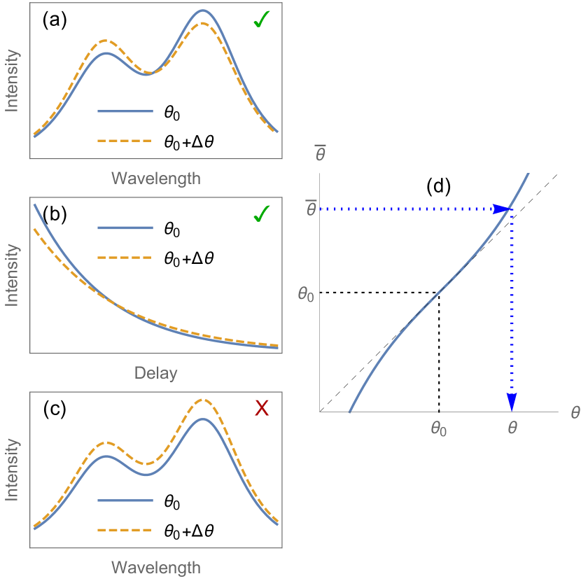
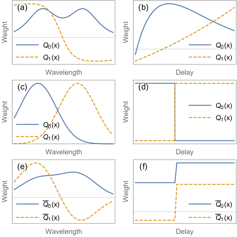
Sensing capabilities of fluorescent nanoparticles can be provided by dependence of their fluorescence lifetime, spectrum, or total intensity on the local parameters of the environment: temperature, pH, pressure, etc. [1, 2, 34, 35, 36, 37, 38, 39] (Fig. 1). Since blinking of the emitters introduces significant noise to the total intensity of fluorescence, we focus on the cases when the environment influences distribution of the fluorescent signal over certain parameter (variable) within the frame. Let be the density of the signal over the variable . Then, the total fluorescent signal for the frame is defined as
| (9) |
For spectral response of the fluorophores to local changes of environment, may correspond to the emitted radiation wavelength and be the spectral density of the signal. For sensing, based on fluorescence lifetime like in the case of SiV centers in diamond needles [39], is the delay between the excitation pulse and the detection of photons.
Eq. (1) can be rewritten in the following form for the density of the signal:
| (10) |
where the dependence on the -th emitter intensity on the variable (wavelength or delay of the fluorescence signal) is affected by the local value of the environment parameter in the vicinity of the -th emitter. To infer the local values of the parameter in question, one needs to specify certain model for the dependence of on and, typically, to assume that all the emitters are described by the same model up to a constant emitter-dependent factor . To eliminate additional noise, caused by blinking of the emitters, it is worth normalizing the signal by dividing it by its integral over .
First, let us assume that the dependence of the emitter’s signal on the parameter of environment is linear in the vicinity of the reference value :
| (11) |
As it is shown in Appendix A, one can build an estimator
| (12) |
where
| (13) |
and ensure, by appropriate choice of the weights and , that the estimator retrieves all the information contained in the intensity profile after its normalization (i.e., represents sufficient statistics).
Eq. (12) indicates the fact that the profile can be “compressed” to just two scalar characteristics (linear functionals)
| (14) |
which are sufficient for retrieving all the available information about the investigated parameter . One can move further and consider the two scalars and for some arbitrary weights and without applying the constraints (13). Practically, those two quantities may correspond to the signal accumulated over two spectral or temporal windows. In that case (see Appendix B), one can still find two linear combinations and of the scalars so that the corresponding weights and satisfy Eq. (13). However, such measurement-induced choice of the weights is, generally, non-optimal and may lead to loss of information relatively to the full profile analysis. The estimator for the environment parameter can be constructed as
| (15) |
where
| (16) |
represent coefficients in decomposition of over powers of the deviation :
| (17) |
In general case, the dependence of on is nonlinear. Considering small deviations , one can linearize and define
| (18) |
Then, following the procedures discussed above, one can construct the weights and and calculate the quantities according to Eq. (14) for the given signal . The dependence of the linear estimator defined by Eq. (15) on the true value of the parameter is, in general, also nonlinear and biased, . Assuming that the dependence is monotonically increasing in certain vicinity of the reference value , one can construct its inverse and build the estimator as
| (19) |
Practically, the procedure means plotting the calibration curve and using it for finding the parameter value for the value calculated from the input data (Fig. 1(d)).
II.3 Combining sensing and SOFI
The proposed idea of combining spatial resolution with sensing consists in applying SOFI separately to several channels relatively to the variable , which defines signal distribution (spectral or temporal) within each frame. Naively, one can just replace the integrated signal by its density in Eq. (4) and get spectrally or temporarily resolved cumulant image:
| (20) |
Practically, such approach would mean that one takes the binned signal density , specified for a discrete set of values , and performs analysis of frame-wise temporal statistics to each bin by considering the time series . However, such time series is unlikely to satisfy the requirement of having enough photons in each frame, which is important for reliable application of SOFI.
Such issue can be resolved by the above-discussed “compression” of a full profile over into several scalar functionals. Following Eq. (14), one can define the signals, integrated over two spectral or temporal windows (indexed as ) within each frame, as follows:
| (21) |
where is calculated according to Eq. (14) for .
In contrast to the binned density , the integrated signals are intense enough to be exploited for SOFI. The cumulants can be constructed for each window separately:
| (22) |
The quantities and have the meaning close to and and can be used for estimation of the local parameter value similarly to Eq. (15). If the deviations of the parameter values at the emitters’ positions from the reference value are small, the factor in Eq. (22) can be decomposed in the way similar to Eq. (17):
| (23) |
Comparison of Eqs. (17) and (23) suggests that one can construct the estimator for the local value of the environment parameter as
| (24) |
Substituting Eqs. (22) and (23) into Eq. (24), one can see that the constructed estimator indeed represents the parameter distribution, blurred by the diffraction:
| (25) |
The effect of blurring reduction for higher-order cumulants, characteristic for SOFI, is still present in Eq. (25): the PSF is raised to the power .
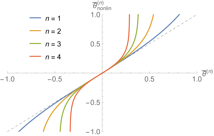
For larger deviations , the nonlinearity of the response should be taken into account similarly to Eq. (19). For a uniform distribution of the parameter (), one has and can find the (nonlinear) dependence of the estimator on the parameter value , calculated according to Eq. (24) with the substitution . Then, in the general case of non-uniform parameter distribution, the nonlinear estimator will be
| (26) |
where is calculated according to Eq. (24). General properties of the estimator are discussed in Appendix C.
II.4 Reconstruction of parameter distribution for noisy signal
While for ideal noiseless data the constructed estimator (26) would provide reasonable local values for the investigated parameter distribution , its application to the noisy data (especially for sparsely located emitters) deserves additional attention. The structure of expression (22) implies that the cumulant values estimated from finite-sample data are more reliable near emitters ( for certain ), but may contain significant relative shot noise contribution in the region between the emitters where the signals are weak. The effect becomes more pronounced for higher-order cumulants, since the effective PSF is narrower for larger , while the contribution of shot noise is generally growing for larger cumulant orders.
The inaccuracy of the reconstructed parameter value is determined by the relative contribution of the shot noise to the quantities and , which is, roughly, inversely proportional to the square root of the detected signal:
| (27) |
The likelihood of getting the estimated distribution for the true distribution can be represented as
| (28) |
In the regions with low signal, the inaccuracy can be large, making the estimate unreliable. The estimate can be refined in the spirit of Tikhonov’s regularization [40]. Very sharp features of the reconstructed distribution of the environment parameter from a blurred image with finite density of fluorescent emitters are likely to be artifacts rather than to provide useful information about the sample. The statement can be captured as a reduced prior probability of the distributions with large values of second derivatives:
| (29) |
where the parameter represents the scale for the derivatives and is 2-dimensional Laplacian.
II.5 Sensing method summary
To realize the proposed sensing approach with spatial super-resolution capabilities, the following procedures should be performed.
1. Model construction. The models for parameter-dependent spectral or temporal profiles of the emitters’ fluorescence and for the emitters’ blinking should be constructed (either theoretically or from empirical calibration procedure).
2. Sensing calibration. The optimal weights and of the two detection channels are defined in Appendix A. If the experimental capabilities do not allow to perform such optimal measurement, the actual weights and are defined by the available detection setup (the profiles of the channels’ sensitivity). For sensing based on the -th order cumulant, the linear estimator is defined according to Eq. (24). The nonlinear relation between the estimator and the true value of the parameter is found by theoretical consideration or direct measurements of the sample response for a uniform distribution of the parameter . The final nonlinear estimator is constructed according to Eq. (26).
3. Data acquisition. The fluorescent response of the sample is collected in terms of 2-channel framed images , where , 1 is the channel index, is the frame index, and is the set of detection positions (pixel positions for an array detector or the scanning positions).
4. Data processing. For each channel and each detection position separately, the cumulant value is calculated. For , 3, 4 the expressions are provided by Eqs. (5)–(7) with the expectation values replaced by finite-sample averages. The local estimates of the parameter are calculated according to Eq. (26).
III Model experiment
III.1 Setup description
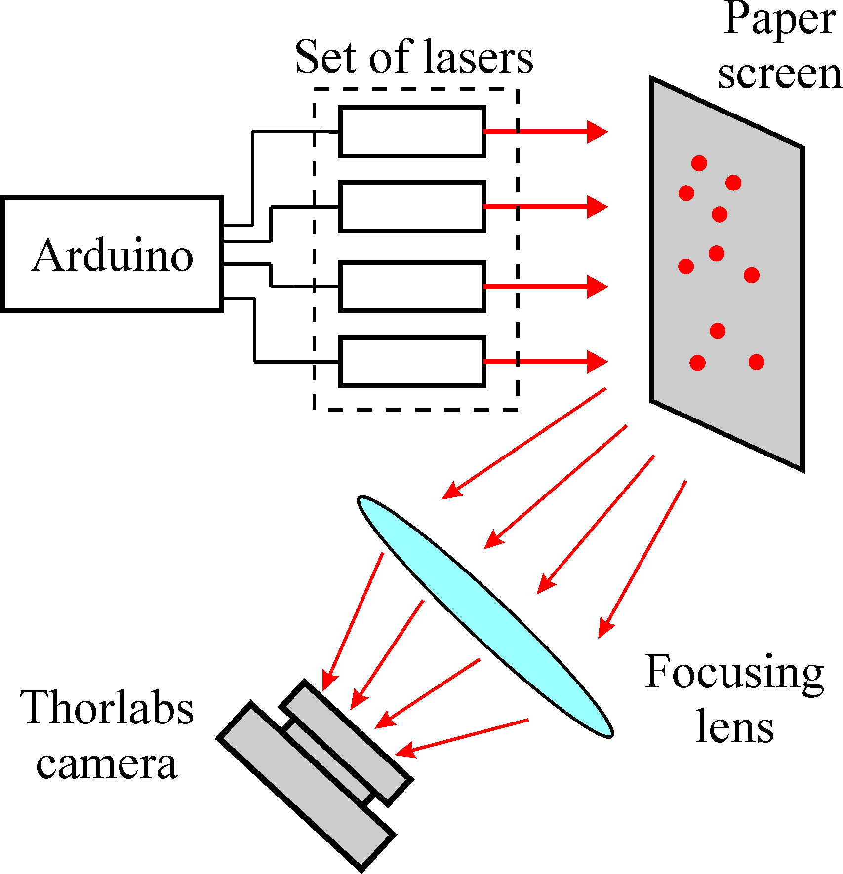
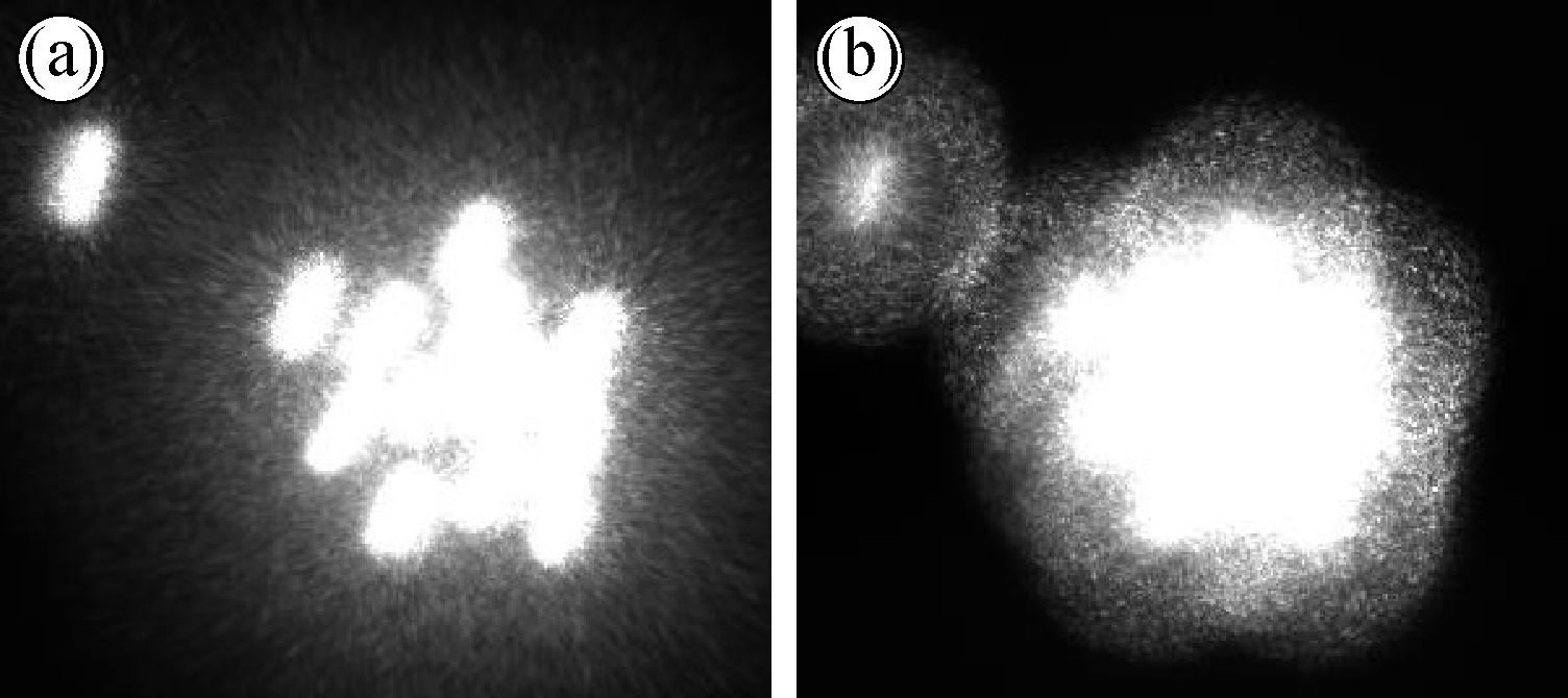
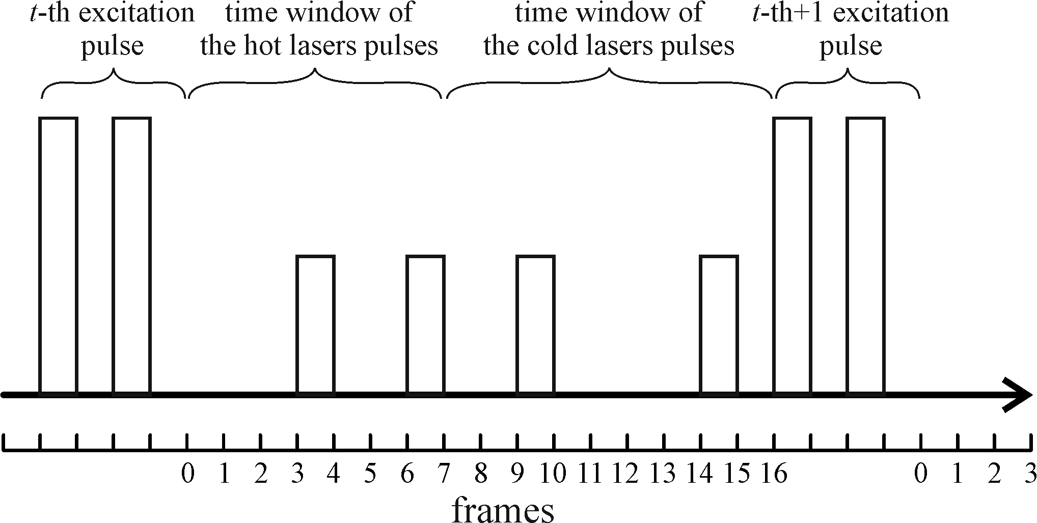
To verify the proposed technique, we performed the following model experiment. We used a paper screen as a model of fluorescent sample. The screen was irradiated with 13 KY-008 lasers controlled by the microcontroller board Arduino MEGA [43]. The image of the screen was recorded with Thorlabs DCC1545M-GL camera with 50 mm lens (Fig. 2). To simulate the diffraction limit, the lens was placed 2 mm closer to the camera than it was necessary to get a clear picture. The images of clear and unfocused laser spots are shown in Fig. 3. Each laser played the role of a fluorescent particle. Correspondingly, each particle had prescribed “relaxation time” meaning the time between “excitation pulse” and “fluorescent emission”. To denote “excitation pulse” in the recording data, Arduino made all lasers blink two times. Since the minimal distinguishable time gap is 1 frame (about 43 ms), we used frames as a measure of time. Therefore, the “excitation pulse” was a series of 2 one-frame flashes of lasers separated by 1 frame of darkness. The “fluorescent emission” was 1-frame flashing of a laser. To simulate the fluorescent particles with different temperature, the lasers were divided into “hot” and “cold” ones. For the hot lasers, the “relaxation time” was 5 frames with standard deviation of 2 frames, while the cold lasers had “relaxation time” of 10 frames with the same standard deviation.
III.2 Data acquisition
The data were recorded in series of 10000 frames with the frame rate of 24 fps. For each “excitation cycle”, each laser was randomly assigned its state (active or dark) and the time delay between the “excitation pulse” and its relaxation (“fluorescent emission”). The delay was sampled according to normal distribution with the mean determined by the model temperature of the laser (“hot” or “cold”). The random sampling was performed by the Arduino microcontroller. Then, Arduino produced an “excitation pulse” and made each active laser to flash after the time delay assigned to it. After modeling “fluorescent emission” of all the active lasers withing the current cycle (when all the lasers are switched off), Arduino waited for 1 frame, and repeated the cycle. In the end, we got a video containing intensity distribution in time and space.
III.3 Data processing and results
First, the recorded video was divided into frames with ffmpeg program [44] and processed with Python script. The script calculated total intensity for each frame and identified “excitation pulses” according to specific alternation of high and low intensity of frames. The frames designating the “excitation pulse” were excluded from further calculations. According to the notations, introduced in Section II, the “excitation cycles” are indexed by , …, .
The signal for each “excitation cycle” was split into two channels and accumulated pixelwise. The “hot” signal is the pixelwise sum of intensities for the 1st - 7th frames after the -th “excitation pulse”, where indices and enumerate pixel positions in each frame. The “cold” signal is defined in the same way starting from the 8th frame after the “excitation pulse” (Fig. 4).
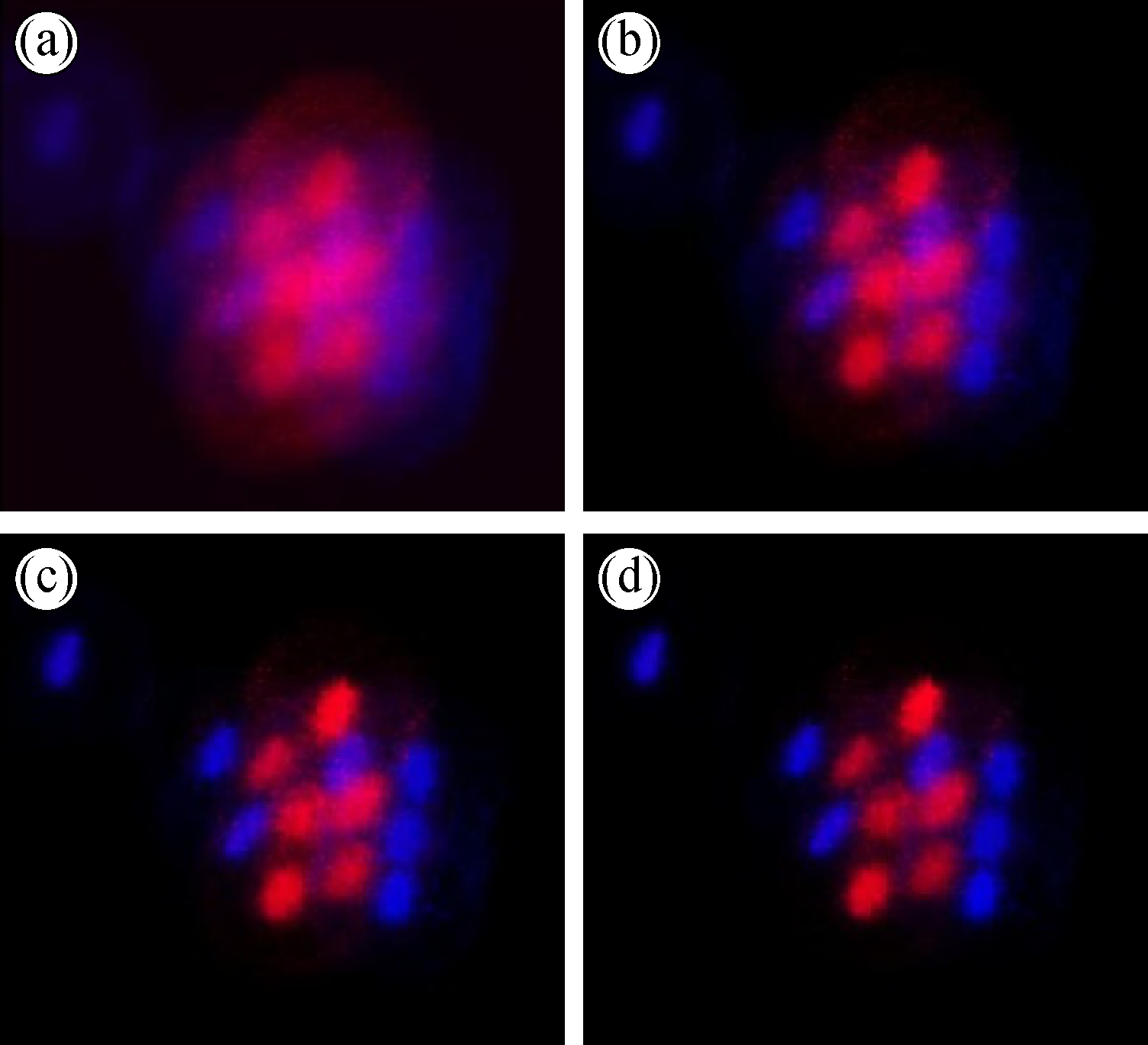
The intensity (mean signal value) and the 2nd, 3rd, and 4th order cumulants for the two channels where defined according to Eqs. (5)–(8). The obtained intensity and cumulant images are shown in Fig. 5. For visualization purposes, the “cold” and “hot” channels were assigned to the blue and red channels of RGB palette respectively. Since the cumulant of the 3rd order can be negative, the absolute value of the cumulant was used to create the image. One can see that the intensity distribution (Fig. 5(a)) is blurred like original unfocused image (Fig. 3(b)). However, it is possible to distinguish the light of “hot” and “cold” lasers because of different relaxation times. The light spots are more visible in the second-order cumulant image (Fig. 5(b)), but the background caused by blurring is still strong. The third-order cumulant image (Fig. 5(c)) is clear enough and the background is hardly visible. The best quality image is given by the fourth-order cumulant (Fig. 5(d)). It allows one to distinguish clearly spots of “hot” and “cold” lasers. To summarize, the experiment is in a good agreement with the theory, and the calculation of cumulants of intensity fluctuations allows one to visualize the particles with different relaxation times.
III.4 Reconstruction of local “temperature”
To fit the above-described model experiment into the theoretical framework, discussed in Section II, we assign the normalized dimensionless “temperature” equal to to “cold” lasers and to “hot” lasers. The emission profile variable corresponds to the camera frame number within the “hyperframe” (excitation cycle) of SOFI in the considered case. For such definitions, the model emission profile is described as
| (32) |
where and the additional parameter-independent background signal is modeled as with and .
A simple threshold filter is used to split the two detection channels:
| (33) |
| (34) |
The decomposition coefficients (Eq. (17)) can be approximated as
| (35) |
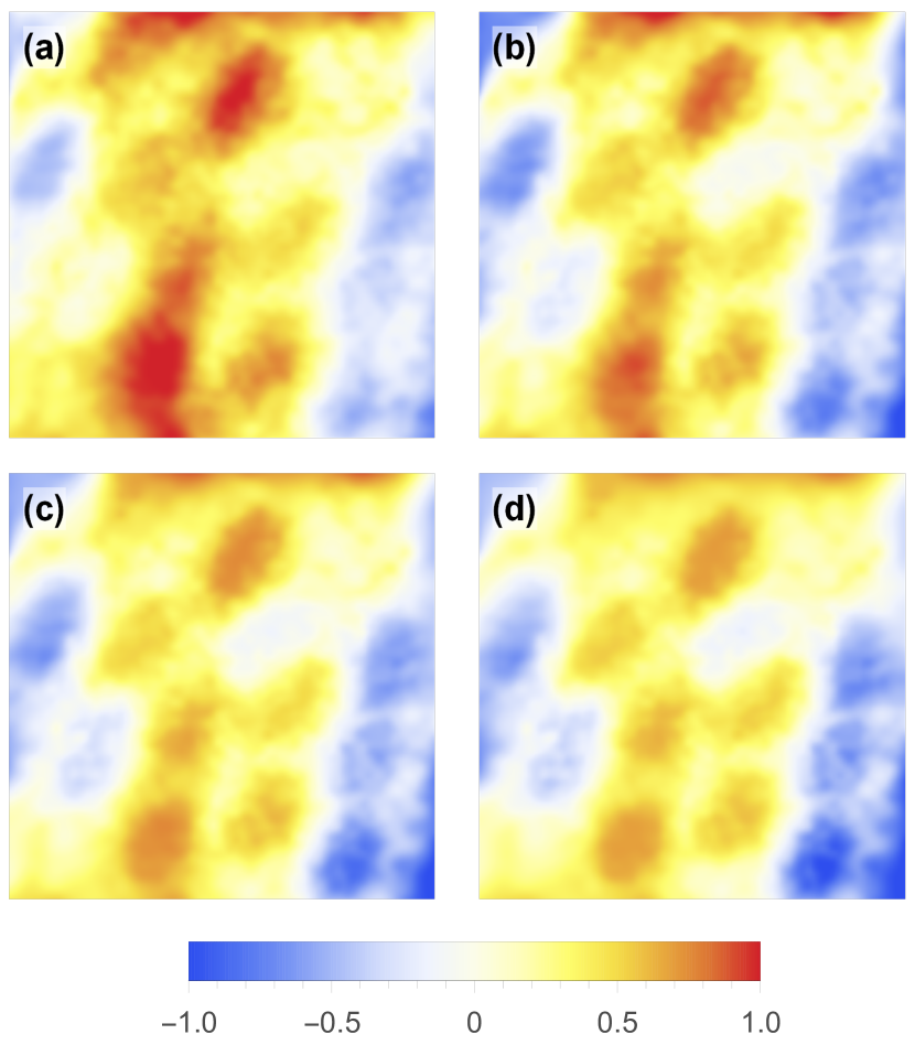
where and 1 correspond to the “” and “” signs respectively. The linear estimator is calculated according to Eq. (24) with , while its more accurate nonlinear counterpart is constructed according to Eq. (26) using the procedure outlined before it (Fig. 6). Further, the reconstructed distribution can be refined using the method outlined in the Section II.4 and Appendix D.
The results are presented in Fig. 7. As predicted, usage of higher-order cumulants enhances spatial resolutions and enables analysis of finer features of the sample. According to the standard performance of SOFI, using fourth order cumulant instead of intensity leads to approximately twice narrower efficient PSF.
IV Discussion
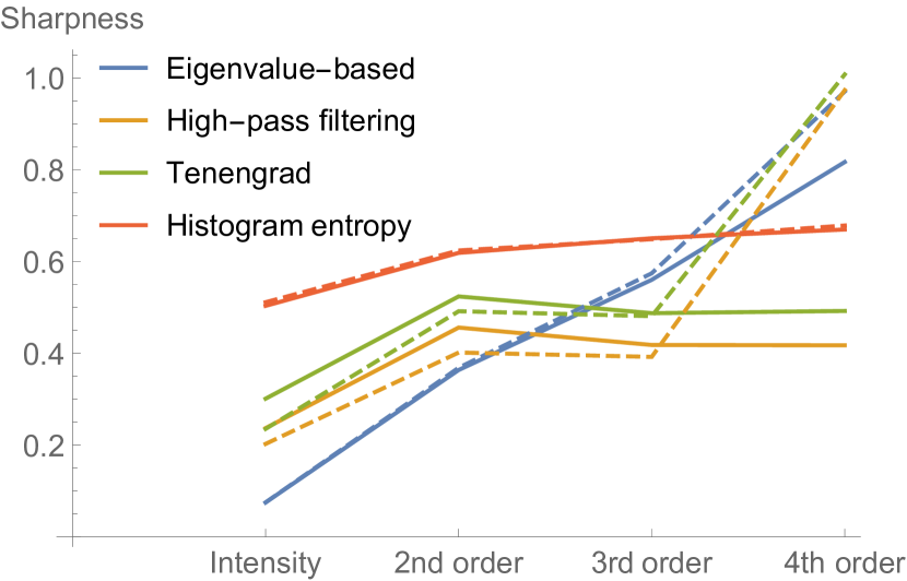
To get quantitative estimates of the proposed approach performance, we applied several sharpness measures to the reconstructed distribution of the local “temperature”. The results shown in Fig. 8 indicate that the most blurred distribution is obtained for the traditional intensity-based approach. Derivative-based measures (Tenengrad and high-pass filtering [45]) give preference to the second-order cumulant (after application of noise-reduction algorithm from subsection II.4), while eigenvalue-based [46] and histogram entropy based [45] methods assign the best score to the fourth-order cumulant.
We believe that the proposed approach and its proof-of-concept experiment can pave the way for:
-
•
detailed analysis and optimization of the combined sensing and imaging approach in terms of classical and quantum Fisher information;
-
•
reconstruction of the sample characteristic distribution by combined usage of several orders of cumulants simultaneously;
-
•
extension of the approach to multimodal sensing, when several characterisics of the sample are reconstructed simultaneously;
-
•
implementation of Fourier spectrum re-weighting for additional de-blurring and cumulant orders combination;
-
•
application of the “sliding window” approach [47] for more efficient processing of many-pixel images.
V Conclusions
We proposed a simple and elegant technique capable of combining sensing with super-resolution imaging, based on non-trivial temporal statistics typical for blinking fluorescent nanoemitters. The approach is universal since the dependence of the fluorophores response on the characteristic to be reconstructed can take different form: changes of the spectrum, fluorescence lifetime, etc. It is shown that splitting the fluorescence signal into just two detection channels at each spatial detection point is sufficient for reliable reconstruction of the local characteristic distribution.
The conducted model experiment proofs soundness and efficiency of the approach and can be used as a guidance for the real-world experiments with, for example, living cells and structured fluorescent nanodiamonds [48] or blinking graphene quantum dots ensembles [49]. In agreement with the theoretical predictions, usage of cumulants instead of emission intensity enhances sharpness of the reconstructed parameter distribution and enables analysis of smaller features of the sample.
Proposed methodology will be useful for local measurements of living cells’ physical parameters, such as temperature, pH, electric field gradient, presence of reactive oxygen spices, i.e. the characteristics which could be recognized as spectral changes of appropriate fluorophore delivered targetly to the wanted cell or even organelle. In its turn, this advanced local sensing tool could give an important insights into fundamental life science, which still lacks instruments capable of monitoring the cellular balance with nanometre spatial resolution to guarantee measurements consistency for that dynamic system.
Acknowledgements.
This study was accomplished through the financial support of Research Council of Finland (Flagship Programme PREIN, decision 320166; research project, decision 357033); QuantERA project EXTRASENS, in Finland funded through Research Council of Finland, decision 361115), Horizon Europe MSCA FLORIN Project 101086142.Appendix A Optimal estimator for linear-response sensing
Here, we show that the information about the environment parameter , contained in the full signal density profile , described by Eq. (11), can be efficiently compressed into two scalar characteristics (Eq. (14)), which are used for building the estimator according to Eq. (12). The analysis is performed in the vicinity of the reference value of the parameter, i.e. the deviation is assumed to be small.
We assume that the signal profile is measured at a discrete set of bins and contains shot noise satisfying Poisson statistics:
| (36) |
where , . To reduce the influence of the noise caused by the emitters’ blinking on the final estimates of the environment parameter, it is useful to consider the normalized signal . The Fisher information of that normalized density profile relatively to the parameter at the point can be calculated as
| (37) |
where the second term describes “information loss” caused by the normalization [50].
For a low level of noise, the estimator (constructed from the noisy signal according to Eq. (12)) is a random variable obeying approximately normal distribution with and . The Fisher information after “compression” of the profile into the scalar equals
| (38) |
Appendix B Practical estimator for sensing with two spectral or temporal windows
In this appendix, we show how scalar characteristics , defined by Eq. (14) without any particular constraints imposed on the weights , can be modified so that Eq. (13) are satisfied.
In general case, the values are decomposed according to Eq. (17). One can construct the following linear combinations of those quantities:
| (43) |
| (44) |
Linearity of Eq. (17) implies that the weights , corresponding to the quantities are related to the initial weights by the same relations:
| (45) |
| (46) |
One can check by direct substitution that the conditions (13) are satisfied for the constructed weights .
Fig. 9 shows an example of weights calculated for the model signal densities depicted in Fig. 1(a,b).
Appendix C General properties of cumulant-based estimator for noiseless data
To be physically reasonable, the estimator , defined by Eq. (26) should satisfy several general requirements when applied to noiseless data.
1. For spatially uniform distribution the estimator should reconstruct the correct value: for all . In that case, according to Eq. (22), one has and, therefore, Eq. (24) retains its value after the replacement . Then, according to the definition (26), the equality holds for all .
2. If the parameter values in the vicinity of the emitters are bounded as , the estimator value is also bounded: for all . According to Eq. (15), the estimator is a function of the ratio , which itself is a function of . The monotonicity of the dependence implies that both of the above-mentioned functions are also monotonic. Therefore, for each emitter, the ratio is bounded by its values at and . The same conclusion is valid for the ratio , since is positive.
Assuming that the blinking statistics is the same for all emitters (i.e., depends only on , but not on ) and taking into account the definition (22), one can conclude that the ratio is bounded by its values for uniform distributions with and for all , too. The derivative of , defined by Eq. (24), over the ratio has constant sign, independent of :
| (47) |
Therefore, the values are also bounded:
| (48) |
Finally, taking into account the definition (26) and monotonicity of , we have
| (49) |
3. If the emitters are evenly distributed (i.e., for each point of interest there is at least one emitter with for some constant ), the parameter estimation by is local:
| (50) |
The statement is valid if the PSF of the imaging system is local:
| (51) |
Then, the relative contribution of a distant emitter to the cumulant value becomes negligible for :
| (52) |
Therefore, it does not influence the value of the estimator .
Appendix D Expressions for regularized parameter estimation
For parameter values, defined at a regular grid , the derivatives in Eq. (29) can be approximated as finite differences. Then, the expression for log-probability takes the form
| (53) |
The sums representing the second and the third terms do not include boundary values of and respectively. The parameter scales as , where is the PSF width expressed in the grid steps and representing the expected minimal size of the reconstructed distribution features, which are not artefacts yet. The proportionality coefficient can be calculated from detailed theoretical investigation of the noise models, but, in practice, it can be just chosen empirically.
Unconstrained minimization of the quantity, defined by the right-hand side of Eq. (53), is trivial and includes just linear inversion according to the least-squares method. One of the approaches to obtaining physically reasonable constrained estimates is to perform constrained quadratic optimization, which, however, becomes much more computationally hard for a large number of grid points . A more efficient way to get reasonable results is to constrain the initial estimate to the range before applying the minimization of the expression (53). If all the values satisfy the constraint , the minimizing set will also belong to the physical range with certainty.
References
- Norman et al. [2021] Victoria A Norman, Sridhar Majety, Zhipan Wang, William H Casey, Nicholas Curro, and Marina Radulaski. Novel color center platforms enabling fundamental scientific discovery. InfoMat, 3(8):869–890, 2021.
- Wu and Weil [2022] Yingke Wu and Tanja Weil. Recent developments of nanodiamond quantum sensors for biological applications. Advanced Science, 9(19):2200059, 2022.
- Radtke et al. [2019] Mariusz Radtke, Ettore Bernardi, Abdallah Slablab, Richard Nelz, and Elke Neu. Nanoscale sensing based on nitrogen vacancy centers in single crystal diamond and nanodiamonds: Achievements and challenges. Nano Futures, 3(4):042004, 2019.
- Xu et al. [2023] Ying Xu, Weiye Zhang, and Chuanshan Tian. Recent advances on applications of nv- magnetometry in condensed matter physics. Photonics Research, 11(3):393–412, 2023.
- Baranov et al. [2011] Pavel G Baranov, Anna P Bundakova, Alexandra A Soltamova, Sergei B Orlinskii, Igor V Borovykh, Rob Zondervan, Rogier Verberk, and Jan Schmidt. Silicon vacancy in sic as a promising quantum system for single-defect and single-photon spectroscopy. Physical Review B, 83(12):125203, 2011.
- Anisimov et al. [2016] AN Anisimov, Dmitrij Simin, VA Soltamov, SP Lebedev, PG Baranov, GV Astakhov, and V Dyakonov. Optical thermometry based on level anticrossing in silicon carbide. Scientific Reports, 6(1):33301, 2016.
- Fu et al. [2007] Chi-Cheng Fu, Hsu-Yang Lee, Kowa Chen, Tsong-Shin Lim, Hsiao-Yun Wu, Po-Keng Lin, Pei-Kuen Wei, Pei-Hsi Tsao, Huan-Cheng Chang, and Wunshain Fann. Characterization and application of single fluorescent nanodiamonds as cellular biomarkers. Proceedings of the National Academy of Sciences, 104(3):727–732, 2007.
- Hui et al. [2010] Yuen Yung Hui, Bailin Zhang, Yuan-Chang Chang, Cheng-Chun Chang, Huan-Cheng Chang, Jui-Hung Hsu, Karen Chang, and Fu-Hsiung Chang. Two-photon fluorescence correlation spectroscopy of lipid-encapsulated fluorescent nanodiamonds in living cells. Optics express, 18(6):5896–5905, 2010.
- Blakley et al. [2015] SM Blakley, IV Fedotov, S Ya Kilin, and AM Zheltikov. Room-temperature magnetic gradiometry with fiber-coupled nitrogen-vacancy centers in diamond. Optics letters, 40(16):3727–3730, 2015.
- Blakley et al. [2016] SM Blakley, IV Fedotov, LV Amitonova, EE Serebryannikov, H Perez, S Ya Kilin, and AM Zheltikov. Fiber-optic vectorial magnetic-field gradiometry by a spatiotemporal differential optical detection of magnetic resonance in nitrogen–vacancy centers in diamond. Optics Letters, 41(9):2057–2060, 2016.
- Chang et al. [2017] K Chang, Alexander Eichler, Jan Rhensius, Luca Lorenzelli, and Christian L Degen. Nanoscale imaging of current density with a single-spin magnetometer. Nano letters, 17(4):2367–2373, 2017.
- Pelliccione et al. [2016] Matthew Pelliccione, Alec Jenkins, Preeti Ovartchaiyapong, Christopher Reetz, Eve Emmanouilidou, Ni Ni, and Ania C Bleszynski Jayich. Scanned probe imaging of nanoscale magnetism at cryogenic temperatures with a single-spin quantum sensor. Nature nanotechnology, 11(8):700–705, 2016.
- Malykhin et al. [2022] Sergei Malykhin, Yuliya Mindarava, Rinat Ismagilov, Fedor Jelezko, and Alexander Obraztsov. Control of nv, siv and gev centers formation in single crystal diamond needles. Diamond and Related Materials, 125:109007, 2022.
- Hell and Wichmann [1994] Stefan W Hell and Jan Wichmann. Breaking the diffraction resolution limit by stimulated emission: stimulated-emission-depletion fluorescence microscopy. Optics letters, 19(11):780–782, 1994.
- Rittweger et al. [2009a] Eva Rittweger, Dominik Wildanger, and SW Hell. Far-field fluorescence nanoscopy of diamond color centers by ground state depletion. Europhysics Letters, 86(1):14001, 2009a.
- Rittweger et al. [2009b] Eva Rittweger, Kyu Young Han, Scott E Irvine, Christian Eggeling, and Stefan W Hell. STED microscopy reveals crystal colour centres with nanometric resolution. Nature Photonics, 3(3):144–147, 2009b.
- Maurer et al. [2010] PC Maurer, Jeronimo R Maze, PL Stanwix, Liang Jiang, Alexey Vyacheslavovich Gorshkov, Alexander A Zibrov, Benjamin Harke, JS Hodges, Alexander S Zibrov, Amir Yacoby, et al. Far-field optical imaging and manipulation of individual spins with nanoscale resolution. Nature Physics, 6(11):912–918, 2010.
- Classen et al. [2017] Anton Classen, Joachim von Zanthier, Marlan O Scully, and Girish S Agarwal. Superresolution via structured illumination quantum correlation microscopy. Optica, 4(6):580–587, 2017.
- Hess et al. [2006] Samuel T Hess, Thanu PK Girirajan, and Michael D Mason. Ultra-high resolution imaging by fluorescence photoactivation localization microscopy. Biophysical journal, 91(11):4258–4272, 2006.
- Rust et al. [2006] Michael J Rust, Mark Bates, and Xiaowei Zhuang. Sub-diffraction-limit imaging by stochastic optical reconstruction microscopy (storm). Nature methods, 3(10):793–796, 2006.
- Schnitzbauer et al. [2017] Joerg Schnitzbauer, Maximilian T Strauss, Thomas Schlichthaerle, Florian Schueder, and Ralf Jungmann. Super-resolution microscopy with dna-paint. Nature protocols, 12(6):1198–1228, 2017.
- Gu et al. [2013] Min Gu, Yaoyu Cao, Stefania Castelletto, Betty Kouskousis, and Xiangping Li. Super-resolving single nitrogen vacancy centers within single nanodiamonds using a localization microscope. Optics express, 21(15):17639–17646, 2013.
- Dertinger et al. [2009] Thomas Dertinger, Ryan Colyer, Gopal Iyer, Shimon Weiss, and Jörg Enderlein. Fast, background-free, 3D super-resolution optical fluctuation imaging (SOFI). Proceedings of the National Academy of Sciences, 106(52):22287–22292, 2009.
- Dertinger et al. [2010] Thomas Dertinger, Ryan Colyer, Robert Vogel, Jörg Enderlein, and Shimon Weiss. Achieving increased resolution and more pixels with superresolution optical fluctuation imaging (SOFI). Optics express, 18(18):18875–18885, 2010.
- Dertinger et al. [2013] Thomas Dertinger, Alessia Pallaoro, Gary Braun, Sonny Ly, Ted A Laurence, and Shimon Weiss. Advances in superresolution optical fluctuation imaging (SOFI). Quarterly reviews of biophysics, 46(2):210–221, 2013.
- Schwartz and Oron [2012] Osip Schwartz and Dan Oron. Improved resolution in fluorescence microscopy using quantum correlations. Physical Review A, 85(3):033812, 2012.
- Schwartz et al. [2013] Osip Schwartz, Jonathan M Levitt, Ron Tenne, Stella Itzhakov, Zvicka Deutsch, and Dan Oron. Superresolution microscopy with quantum emitters. Nano Letters, 13(12):5832–5836, 2013.
- Monticone et al. [2014] D Gatto Monticone, K Katamadze, Paolo Traina, E Moreva, Jacopo Forneris, Ivano Ruo-Berchera, Paolo Olivero, IP Degiovanni, Giorgio Brida, and M Genovese. Beating the abbe diffraction limit in confocal microscopy via nonclassical photon statistics. Physical Review Letters, 113(14):143602, 2014.
- Gallina et al. [2013] Maria Elena Gallina, Jianmin Xu, Thomas Dertinger, Adva Aizer, Yaron Shav-Tal, and Shimon Weiss. Resolving the spatial relationship between intracellular components by dual color super resolution optical fluctuations imaging (sofi). Optical Nanoscopy, 2(1):1–9, 2013.
- Grußmayer et al. [2020] Kristin S Grußmayer, Stefan Geissbuehler, Adrien Descloux, Tomas Lukes, Marcel Leutenegger, Aleksandra Radenovic, and Theo Lasser. Spectral cross-cumulants for multicolor super-resolved sofi imaging. Nature Communications, 11(1):3023, 2020.
- Liu et al. [2020] Zhihe Liu, Jie Liu, Zhe Zhang, Zezhou Sun, Xuyang Shao, Jintong Guo, Lei Xi, Zhen Yuan, Xuanjun Zhang, Daniel T Chiu, et al. Narrow-band polymer dots with pronounced fluorescence fluctuations for dual-color super-resolution imaging. Nanoscale, 12(14):7522–7526, 2020.
- Glogger et al. [2021] Marius Glogger, Christoph Spahn, Jörg Enderlein, and Mike Heilemann. Multi-color, bleaching-resistant super-resolution optical fluctuation imaging with oligonucleotide-based exchangeable fluorophores. Angewandte Chemie, 133(12):6380–6383, 2021.
- Horoshko et al. [2024] D. Horoshko, M. Kolobov, A. Mikhalychev, and P. Kuzhir. Fisher information analysis for localisation of blinking sources of light. To be published, 2024.
- Bushuev et al. [2016] EV Bushuev, V Yu Yurov, AP Bolshakov, VG Ralchenko, EE Ashkinazi, AV Ryabova, IA Antonova, PV Volkov, AV Goryunov, and A Yu Luk’yanov. Synthesis of single crystal diamond by microwave plasma assisted chemical vapor deposition with in situ low-coherence interferometric control of growth rate. Diamond and Related Materials, 66:83–89, 2016.
- Maletinsky et al. [2012] Patrick Maletinsky, Sungkun Hong, Michael Sean Grinolds, Birgit Hausmann, Mikhail D Lukin, Ronald L Walsworth, Marko Loncar, and Amir Yacoby. A robust scanning diamond sensor for nanoscale imaging with single nitrogen-vacancy centres. Nature nanotechnology, 7(5):320–324, 2012.
- Arcizet et al. [2011] Olivier Arcizet, Vincent Jacques, Alessandro Siria, Philippe Poncharal, Pascal Vincent, and Signe Seidelin. A single nitrogen-vacancy defect coupled to a nanomechanical oscillator. Nature Physics, 7(11):879–883, 2011.
- Babinec et al. [2010] Thomas M Babinec, Birgit JM Hausmann, Mughees Khan, Yinan Zhang, Jeronimo R Maze, Philip R Hemmer, and Marko Lončar. A diamond nanowire single-photon source. Nature nanotechnology, 5(3):195–199, 2010.
- Lesik et al. [2013] Margarita Lesik, Piernicola Spinicelli, Sébastien Pezzagna, Patrick Happel, Vincent Jacques, Olivier Salord, Bernard Rasser, Anne Delobbe, Pierre Sudraud, Alexandre Tallaire, et al. Maskless and targeted creation of arrays of colour centres in diamond using focused ion beam technology. physica status solidi (a), 210(10):2055–2059, 2013.
- Golubewa et al. [2022] Lena Golubewa, Yaraslau Padrez, Sergei Malykhin, Tatsiana Kulahava, Ekaterina Shamova, Igor Timoshchenko, Marius Franckevicius, Algirdas Selskis, Renata Karpicz, Alexander Obraztsov, et al. All-optical thermometry with NV and SiV color centers in biocompatible diamond microneedles. Advanced Optical Materials, 10(15):2200631, 2022.
- Tikhonov and Arsenin [1977] Andrey N Tikhonov and Vasiliy Y Arsenin. Solutions of ill-posed problems. Washington, DC: John Wiley & Sons, New York, 1977.
- Gelman et al. [2013] A. Gelman, J. B. Carlin, H. S. Stern, and D. B. Dunson. Bayesian data analysis. Chapman and Hall/CRC, 2013.
- Koch [2007] K.-R. Koch. Introduction to Bayesian statistics. Springer Science & Business Media, 2007.
- [43] Arduino hardware and software. https://www.arduino.cc.
- [44] A complete, cross-platform solution to record, convert and stream audio and video. https://ffmpeg.org.
- Krotkov [1988] Eric Krotkov. Focusing. International Journal of Computer Vision, 1(3):223–237, 1988.
- Wee and Paramesran [2007] Chong-Yaw Wee and Raveendran Paramesran. Measure of image sharpness using eigenvalues. Information Sciences, 177(12):2533–2552, 2007.
- Mikhalychev et al. [2019] AB Mikhalychev, B Bessire, IL Karuseichyk, AA Sakovich, M Unternährer, DA Lyakhov, Dominik L Michels, André Stefanov, and D Mogilevtsev. Efficiently reconstructing compound objects by quantum imaging with higher-order correlation functions. Communications Physics, 2(1):134, 2019.
- Quarshie et al. [2024] Mariam M Quarshie, Sergei Malykhin, Alexander Obraztsov, and Polina Kuzhir. Nano-and micro-crystalline diamond film structuring with electron beam lithography mask. Nanotechnology, 35(15):155301, 2024.
- Belko et al. [2022] Nikita Belko, Lena Golubewa, Vyacheslav Chizhevsky, Sopfy Karuseichyk, Dmitry Filimonenko, Marija Jankunec, Hamza Rehman, Tatsiana Kulahava, Polina Kuzhir, and Dmitri Mogilevtsev. Hysteresis and stochastic fluorescence by aggregated ensembles of graphene quantum dots. The Journal of Physical Chemistry C, 126(25):10469–10477, 2022.
- Mikhalychev et al. [2021] Alexander Mikhalychev, Konstantin Zhevno, Svetlana Vlasenko, Andrei Benediktovitch, Tatjana Ulyanenkova, and Alex Ulyanenkov. Fisher information for optimal planning of x-ray diffraction experiments. Journal of Applied Crystallography, 54(6):1676–1697, 2021.
- Lehmann and Casella [2006] Erich L Lehmann and George Casella. Theory of point estimation. Springer, 2006.
- Cohen [1968] M Cohen. The Fisher information and convexity. IEEE Trans. Inf. Theory, 14(4):591–592, 1968.