Robustness-Congruent Adversarial Training for Secure Machine Learning Model Updates

Abstract

Machine-learning models demand for periodic updates to improve their average accuracy, exploiting novel architectures and additional data. However, a newly-updated model may commit mistakes that the previous model did not make. Such misclassifications are referred to as negative flips, and experienced by users as a regression of performance. In this work, we show that this problem also affects robustness to adversarial examples, thereby hindering the development of secure model update practices. In particular, when updating a model to improve its adversarial robustness, some previously-ineffective adversarial examples may become misclassified, causing a regression in the perceived security of the system. We propose a novel technique, named robustness-congruent adversarial training, to address this issue. It amounts to fine-tuning a model with adversarial training, while constraining it to retain higher robustness on the adversarial examples that were correctly classified before the update. We show that our algorithm and, more generally, learning with non-regression constraints, provides a theoretically-grounded framework to train consistent estimators. Our experiments on robust models for computer vision confirm that (i) both accuracy and robustness, even if improved after model update, can be affected by negative flips, and (ii) our robustness-congruent adversarial training can mitigate the problem, outperforming competing baseline methods.

1 Introduction

Many modern applications of machine learning require frequent model updates to keep pace with the introduction of novel and more powerful architectures, as well as with changes in the underlying data distribution. For instance, when dealing with cybersecurity-related tasks like malware detection, novel threats are discovered at a high pace, and machine learning models need to be constantly retrained to learn to detect them with high accuracy. Another example is given by image tagging, in which image classification and detection models are used to tag pictures of users, and the variety of depicted objects and scenarios varies over time, requiring constant updates. In both cases, as novel and more powerful machine learning architectures emerge, they are rapidly adopted to improve the average system performance; consider, for instance, the need for transitioning from convolutional neural networks to transformer-based architectures.

Within the aforementioned scenarios, the practice of delivering frequent model updates opens up a new challenge related to the maintenance of machine learning models and their performance as perceived by the end users. The issue is that average accuracy is not elaborate enough to also account for sample-wise performance. In particular, even if average accuracy increases after update, some samples that were correctly predicted by the previous model might be misclassified after model update. There is indeed no guarantee that a newly-updated model with higher average accuracy will not commit any mistake on the samples that were correctly predicted by the previous model. The samples that were correctly predicted by the previous model and become misclassified after update have been referred to as Negative Flips (NFs) in [1]. Such mistakes are perceived by end users and practitioners as a regression of performance, similarly to what happens in classical software development, where the term “regression” refers to the deterioration of performance after an update. For this reason, reducing negative flips when performing model updates can be considered as important in practice as improving the overall system accuracy. To better understand the relevance of this issue, consider again the case of malware detection. Experiencing NFs in this domain amounts to having either previously-known legitimate samples misclassified as false positives, or previously-detected malware samples misclassified as legitimate, increasing the likelihood of infecting devices in the wild. Similarly, for the case of image tagging, users might find some of their photos changing labels and potentially being mislabeled after a model update, resulting in a bad user experience. Yan et al. [1] have been the first to highlight this issue, and proposed an approach aimed at minimizing negative flips, referred to as Positive Congruent Training (PCT). The underlying idea of their method is to include an additional knowledge-distillation loss while training the updated model to retain the behavior of the old model on samples that were correctly classified before model update. This forces the updated model to reduce the number of errors on such samples (i.e., the number of negative flips), while also aiming to improve the average classification accuracy.

In this work, we argue that model updates may not only induce a perceived regression of classification accuracy via negative flips, but also a regression of other trustworthiness-related metrics, including adversarial robustness. Adversarial robustness is the ability of machine learning models to withstand adversarial examples, i.e., inputs carefully perturbed to mislead classification at test time. Recent progress has shown that adversarial robustness can be improved by adopting more recent neural network architectures and data augmentation techniques [2]. When updating the system with a more recent and robust model, one is expected to gain an overall increase in robust accuracy, i.e., the fraction of adversarial examples (crafted within a given perturbation budget) that are correctly classified by the model. However, similarly to the case of classification accuracy, some previously-ineffective adversarial examples may be able to evade the newly-updated model, thereby causing a perceived regression of robustness. We refer to these newly-induced mistakes as robustness negative flips (RNFs) in the remainder of this manuscript. We discuss the different types of regression in machine learning in Sect. 2.

Our contribution is twofold. We are the first to show that the update of robust machine-learning models can cause a perceived regression of their robustness, meaning that the new model may be fooled by adversarial examples which the previous model was robust to. Furthermore, we propose a novel technique named robustness-congruent adversarial training (RCAT) to overcome this issue, presented in Sect. 3. As the name suggests, our methodology utilizes the well-known adversarial training (AT) procedure to update machine learning models by incorporating adversarial examples within their training data [3]. In particular, we enrich AT by re-formulating the optimization problem with an additional non-regression penalty term that forces the model to retain high robustness on previously-detected adversarial examples, minimizing the fraction of robustness negative flips (as well as the fraction of negative flips). Finally, we show that our technique is also theoretically grounded, demonstrating that learning with a non-regression constraint provides a statistically-consistent estimator, without even affecting the usual convergence rate of $O(\nicefrac{{1}}{{\sqrt{n}}})$, where $n$ is the number of training samples.

Our experiments, reported in Sect. 4, confirm the presence of regression when updating robust models, showing that state-of-the-art image classifiers [2] with higher robustness than their predecessors are misled by some previously-detected adversarial examples. We further show that, when updating models using our RCAT approach, we are able to improve the accuracy and robustness of the updated models while containing both negative flips and robustness negative flips, outperforming competing baselines. We discuss related work on backward compatibility of machine-learning models and continual learning in Sect. 5, and conclude the paper by discussing limitations of the current approach and future research directions in Sect. 6.

2 Regression of Machine Learning Models

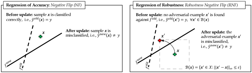
Figure 1: Regression modes in machine-learning model updates. Left: Regression of accuracy induced by negative flips (NFs). When updating an old model $f^{\rm old}$ (dashed black line) with a new model $f^{\rm new}$ (solid black line), a test sample $\boldsymbol{x}$ that was correctly classified by $f^{\rm old}$ may be misclassified by $f^{\rm new}$, causing an NF. Right: Regression of robustness induced by robustness negative flips (RNFs). In a different setting, the test sample $\boldsymbol{x}$ may be still correctly classified by $f^{\rm new}$. However, while no adversarial examples are found against $f^{\rm old}$ (since the perturbation domain $\mathcal{B}(\boldsymbol{x})$, represented by the dashed gray box around $\boldsymbol{x}$, never intersects the decision boundary of $f^{\rm old}$), the adversarial example $\boldsymbol{x}^{\prime}$ is misclassified by $f^{\rm new}$, causing an RNF.

Before delving into the discussion about the types of regression which may be experienced when updating machine learning models, we define some basic notation that will be used throughout this manuscript.

Notation. Let us denote with $\mathcal{D}=(\boldsymbol{x}_{i},y_{i})_{i=1}^{n}$ the training set, consisting of $n$ $d$-dimensional samples $\boldsymbol{x}_{i}\in\mathcal{X}\subseteq\mathbb{R}^{d}$, along with their class labels $y_{i}\in\mathcal{Y}=\{1,\ldots,c\}$. We similarly define the test set as $\mathcal{T}=(\boldsymbol{x}_{j},y_{j})_{j=1}^{m}$, and assume that both datasets are sampled from the same, unknown probability distribution. Accordingly, a machine learning model can be represented as a function $f:\mathcal{X}\mapsto\mathbb{R}^{c}$, which outputs a confidence value for each class (also referred to as logit). For compactness, we will also use $f_{k}(\boldsymbol{x})$ to denote the confidence value associated to class $k$. The predicted class label can be thus denoted with $\hat{y}(\boldsymbol{x})=\arg\max_{k\in\mathcal{Y}}f_{k}(\boldsymbol{x})$, where the dependency of $\hat{y}$ on $\boldsymbol{x}$ may be omitted in some cases to keep the notation uncluttered. Training a model amounts to finding a function $f$ within a feasible set $\mathcal{F}$ (e.g., constrained by a fixed network architecture) that minimizes a loss $L(y,f(\boldsymbol{x}))$ on the training samples in $\mathcal{D}$, typically using a convex loss that provides an upper bound on the classification error (i.e., the zero-one loss), while penalizing complex solutions via a regularization term that prevents overfitting. This helps to find solutions that achieve lower error on the test set $\mathcal{T}$ and are thus expected to generalize better.

2.1 Regression of Accuracy: Negative Flips (NFs)

Training a model by minimizing the aforementioned objective means finding a suitable set of parameters for $f$ that reduces the probability of misclassification over all samples. However, this formulation does not constrain the behavior of the model on specific samples, or in specific regions of the feature space. Thus, when updating an old model $f^{\rm old}$ with a new model $f^{\rm new}$ that is trained on the same data $\mathcal{D}$ but using a different network architecture, one may observe that $f^{\rm new}$ yields a lower classification error on $\mathcal{T}$ while misclassifying different samples than those that were misclassified by $f^{\rm old}$. In other words, there might be some test samples $\boldsymbol{x}$ for which $\hat{y}^{\rm old}(\boldsymbol{x})=y$ and $\hat{y}^{\rm new}(\boldsymbol{x})\neq y$, being $y$ their true class. These samples are referred to as negative flips (NFs), as they are responsible for worsening the performance of the new model when compared to the old one. Conversely, the samples that were misclassified by the old model but not by the new one are referred to as positive flips as they improve the overall accuracy of $f^{\rm new}$ on $\mathcal{T}$. More formally, we can define the NF rate (measured on the test set $\mathcal{T}$) as suggested by Yan et al. [1]:

$${\rm NF(\%)}=\frac{1}{m}\sum_{j=1}^{m}\mathbb{I}\left(\hat{y}_{j}^{\rm old}=y_{j}\land\hat{y}_{j}^{\rm new}\neq y_{j}\right)\,,$$ (1)

where $\mathbb{I}$ is the indicator function, which equals one only if the input statement holds true (and zero otherwise), $\land$ is the logical and operator, and we make use of the compact notation $\hat{y}_{j}^{\rm old}$ and $\hat{y}_{j}^{\rm new}$ to denote respectively $\hat{y}^{\rm old}(\boldsymbol{x}_{j})$ and $\hat{y}^{\rm new}(\boldsymbol{x}_{j})$. The regression of accuracy induced by NFs after model update is also exemplified in Fig. 1 (left).

2.1.1 Positive-Congruent Training (PCT)

To reduce the presence of NFs after model update, and prevent the system users from experiencing a regression of accuracy when using the new model, Yan et al. [1] proposed a technique named Positive-Congruent Training (PCT). The underlying idea of PCT is to add a knowledge-distillation term to the loss function optimized when training the new model $f^{\rm new}$. This term is referred to as focal distillation, as it forces $f^{\rm new}$ to produce similar outputs to those of $f^{\rm old}$ on the samples that were correctly classified by the old model. The PCT approach can be formally described as:

$$f^{\rm new}\in\operatornamewithlimits{\arg\,\min}_{f\in\mathcal{F}}\sum_{i=1}^{n}L(y_{i},f(\boldsymbol{x}_{i}))+\lambda\cdot L_{FD}(f(\boldsymbol{x}_{i}),f^{\rm old}(\boldsymbol{x}_{i}))\,,$$ (2)

being $L$ a standard loss function (e.g., the cross-entropy loss), $L_{FD}$ the focal-distillation loss, and $\lambda$ a trade-off hyperparameter. The focal-distillation loss takes the logits $f(\boldsymbol{x}_{i})$ of the new model $f$ being optimized as inputs, along with the logits $f^{\rm old}(\boldsymbol{x}_{i})$ provided by the old model, and it is computed as:

$$L_{FD}=\left(\alpha+\beta\cdot\mathbb{I}(\hat{y}^{\rm old}_{i}=y_{i})\right)\cdot L_{D}(f(\boldsymbol{x}_{i}),f^{\rm old}(\boldsymbol{x}_{i}))\,,$$ (3)

where $\alpha$ and $\beta$ are two (non-negative) hyperparameters, and $L_{D}$ is the distillation loss. The hyperparameter $\alpha$ forces the distillation of the old model over the whole sample set, while $\beta$ is used to upweight the contribution of the samples that were correctly classified by $f^{\rm old}$. In this manner, the new model tends to mimic the behavior of the old model where the latter performed correctly, reducing the potential mistakes induced by NFs. While in their work Yan et al. [1] experimented with different distillation losses, we focus here on the most promising one, named focal distillation with logit matching (FD-LM). This distillation loss simply measures the squared Euclidean distance between the logits of the model $f$ being optimized and those of the old model $f^{\rm old}$:

$$L_{D}(f(\boldsymbol{x}_{i}),f^{\rm old}(\boldsymbol{x}_{i}))=\frac{1}{2}\|f(\boldsymbol{x}_{i})-f^{\rm old}(\boldsymbol{x}_{i})\|_{2}^{2}.$$ (4)

While PCT has empirically proven to reduce NFs, it has not been designed to deal with the regression of robustness. Furthermore, its theoretical properties have not been analyzed, and it remains thus unclear whether it provides a sound, statistically-consistent estimator.

2.2 Regression of Robustness: Robustness Negative Flips (RNFs)

After introducing the notion of regression of accuracy, induced by the presence of NFs after model update, we argue here that incremental changes to machine-learning models can also affect their security against adversarial examples [4, 5], i.e., carefully-crafted input perturbations aimed to cause misclassifications at test time. More formally, adversarial examples are found by solving the following optimization:

$$\max_{\boldsymbol{x}^{\prime}\in\mathcal{B}(\boldsymbol{x})}L(y,f(\boldsymbol{x}^{\prime}))\,,$$ (5)

where $\mathcal{B}(\boldsymbol{x})=\{\boldsymbol{x}^{\prime}\in\mathcal{X}:\|\boldsymbol{x}^{\prime}-\boldsymbol{x}\|_{p}\leq\varepsilon\}$ defines the perturbation domain, $\|\cdot\|_{p}$ a suitable $\ell_{p}$ norm, and $\varepsilon$ the perturbation budget. In practice, the goal is to find a sample $\boldsymbol{x}^{\prime}\in\mathcal{B}(\boldsymbol{x})$ that is misclassified by $f$, i.e., for which $\hat{y}(\boldsymbol{x}^{\prime})\neq y$.

As shown in Fig. 1 (right), the adversarial example $\boldsymbol{x}^{\prime}$ is optimized within an $\ell_{\infty}$-norm (box) constraint of radius $\varepsilon$ centered on the source sample $\boldsymbol{x}$. It is not difficult to see that, while no adversarial example can be found against the old model $f^{\rm old}$ (as the box constraint never intersects its decision boundary), the same does not hold for the new model $f^{\rm new}$, which is evaded by the adversarial example $\boldsymbol{x}^{\prime}$. Accordingly, when updating the old model $f^{\rm old}$ with $f^{\rm new}$, even if the overall robust accuracy may increase, it may happen that the $f^{\rm new}$ is evaded by some adversarial examples that were not found against $f^{\rm old}$, causing what we call robustness negative flips (RNFs). More formally, we define the RNF rate as:

$${\rm RNF(\%)}=\frac{1}{m}\sum_{j=1}^{m}\mathbb{I}\left(\hat{y}^{\rm old}(\boldsymbol{x}_{j}^{\prime})=y_{j}\land\hat{y}^{\rm new}(\boldsymbol{x}_{j}^{\prime\prime})\neq y_{j}\right)\,,$$ (6)

where $\boldsymbol{x}_{j}^{\prime}$ and $\boldsymbol{x}_{j}^{\prime\prime}$ are the adversarial examples obtained by solving Problem (5) against $f^{\rm old}$ and $f^{\rm new}$, respectively. This means that adversarial examples are re-optimized against each model, and the statement $\hat{y}^{\rm old}(\boldsymbol{x}_{j}^{\prime})=y_{j}$ holds true only if no adversarial example within the given perturbation domain $\mathcal{B}(\boldsymbol{x})$ is found against $f^{\rm old}$, i.e., no sample in $\mathcal{B}(\boldsymbol{x})$ is misclassified by $f^{\rm old}$, whereas it suffices to find one evasive sample against $f^{\rm new}$ to conclude that $\hat{y}^{\rm new}(\boldsymbol{x}_{j}^{\prime\prime})\neq y_{j}$. This makes measuring regression of robustness more complex, as it is defined over a perturbation domain $\mathcal{B}(\boldsymbol{x})$ around each input sample $\boldsymbol{x}$, rather than just on the set of input samples. However, as we will see in our experiments, it can be reliably estimated using state-of-the-art attack algorithms and best practices to optimize adversarial examples [6, 7, 8].

To conclude, note that an input sample $\boldsymbol{x}$ may be correctly classified by $f^{\rm old}$, and at the same time no corresponding adversarial example may exist, i.e., no $\boldsymbol{x}^{\prime}$ evading $f^{\rm old}$ can be found within the given perturbation domain $\mathcal{B}(\boldsymbol{x})$, as shown in the right plot of Fig. 1. After update, it may happen that $f^{\rm new}$ misclassifies the input sample $\boldsymbol{x}$. Thus, by definition, $\boldsymbol{x}$ coincides with the solution of Problem (5), i.e., its adversarial example $\boldsymbol{x}^{\prime}$. This case will be accounted both as an NF and as an RNF. However, as we will show in our experiments, these joint negative flips are typically very rare and overall negligible.

3 Secure Model Updates via Robustness-Congruent Adversarial Training

We present here our Robustness-Congruent Adversarial Training (RCAT) approach to updating machine-learning models while keeping a low number of NFs and RNFs (Sect. 3.1). We then demonstrate how RCAT, as well as PCT, provide statistically-consistent estimators in Sect. 3.2.

3.1 Robustness-Congruent Adversarial Training

We formulate RCAT as an extension of Problem (2) that includes adversarial training, i.e., the optimization of adversarial examples during model training. This is a well-known practice used to improve adversarial robustness of machine-learning models [3]. Before introducing RCAT, we propose a trivial extension of PCT with adversarial training, which we refer to as Positive-Congruent Adversarial Training (PCAT).

Positive-Congruent Adversarial Training (PCAT). PCAT amounts to solving the following problem:

$$\min_{f\in\mathcal{F}}\sum_{i=1}^{n}\max_{\boldsymbol{x}_{i}^{\prime}\in\mathcal{B}_{i}}L(y_{i},f(\boldsymbol{x}_{i}^{\prime}))+\lambda\cdot L_{FD}(f(\boldsymbol{x}_{i}^{\prime}),f^{\rm old}(\boldsymbol{x}_{i}^{\prime}))\,,$$ (7)

where $\mathcal{B}_{i}$ is used to compactly denote $\mathcal{B}(\boldsymbol{x}_{i})$. This is a min-max optimization problem that aims to find the worst-case adversarial example $\boldsymbol{x}_{i}^{\prime}$ for each training sample $\boldsymbol{x}_{i}$, while upweighting the distillation loss on the adversarial examples that were not able to fool $f^{\rm old}$. The underlying idea is to preserve robustness on the samples for which no adversarial example was found against $f^{\rm old}$, thereby reducing RNFs. However, as we will show in our experiments, this technique is not very effective in preventing regression of robustness, even though it provides a reasonable baseline for comparison. In particular, the main problems that arise when trying to use PCAT are: (i) it is not easy to define an effective hyperparameter tuning strategy; and (ii) it is not possible to exploit an already-trained, updated, and more robust model directly.

Robustness-Congruent Adversarial Training (RCAT). With respect to the baseline idea of PCAT, we define RCAT as:

$$\min_{f\in\mathcal{F}}\sum_{i=1}^{n}\max_{\boldsymbol{x}^{\prime}_{i}\in\mathcal{B}_{i}}\gamma\cdot L(y_{i},f(\boldsymbol{x}^{\prime}_{i}))+\alpha\cdot L_{D}(f({\boldsymbol{x}}_{i}^{\prime}),f^{\rm src}({\boldsymbol{x}}^{\prime}_{i}))\,+$$

$$\beta\cdot\mathbb{I}(\hat{y}^{\rm old}(\boldsymbol{x}^{\prime}_{i})=y_{i})\cdot L_{D}(f({\boldsymbol{x}}^{\prime}_{i}),f^{\rm old}({\boldsymbol{x}}^{\prime}_{i}))\,.$$ (8)

This formulation presents two main changes with respect to PCAT (Problem 7), to overcome the two aforementioned limitations of such method. First, to facilitate hyperparameter tuning, we redefine the range of the hyperparameters $\alpha,\beta\in[0,1]$, while fixing $\gamma=1-\alpha-\beta$, so that the three hyperparameters sum up to 1. We also remove the hyperparameter $\lambda$ as it is redundant. Second, we use $f^{\rm src}$ instead of $f^{\rm old}$ in the $\alpha$-scaled term of the focal distillation loss (Eq. 3). The reason is that one may want to update a model $f^{\rm old}$ with an already-trained source model $f^{\rm src}$ that exhibits improved accuracy and robustness, while also reducing NFs and RNFs after update. As $f^{\rm src}$ can be used to initialize $f$ before training via RCAT, it is not reasonable to enforce the behavior of $f^{\rm old}$ over the whole input space. We can indeed try to preserve the behavior of the improved $f^{\rm src}$ model over the whole input space, while enforcing that of $f^{\rm old}$ only on those regions of the input space in which no adversarial examples against $f^{\rm old}$ are found. This is especially convenient when dealing with robust models, as they are normally trained with complicated variants of adversarial training and data augmentation, resulting in a significant computational complexity increase. Thus, if an already-trained, more robust model becomes available, it can be readily used in RCAT as $f^{\rm src}$, as well as to initialize $f$ before optimizing it, while $f^{\rm old}$ can be used to reduce NFs and RNFs in the $\beta$-scaled term.

To summarize, with respect to the baseline PCT formulation in Eq. (2) [1], RCAT provides the following modifications:

1. it includes an adversarial training loop to reduce RNFs;

2. it redefines the hyperparameters to facilitate tuning; and

3. it gives the possibility of distilling from a different model than $f^{\rm old}$ over the whole input space, when available, to retain better accuracy and robustness.

Input :  $\mathcal{D}$, the training dataset; $\mathcal{L}$, the loss defined in Eq. 8, with its fixed hyperparameters $\alpha$, and $\beta$; $f^{\rm src}$, the source/init model; $f^{\rm old}$, the old model; $a$, the attack algorithm used to solve the inner maximization in Eq. (8) over $\mathcal{B}$, the perturbation domain; $\eta$, the learning rate; and $E$, the number of epochs;

Output : $f^{\rm new}$, the model trained with RCAT.

1

$f_{\boldsymbol{w}}\leftarrow f^{\rm src}$

  $\triangleright$ Initialize the model as $f^{\rm src}$

2

3for $i\in[1,E]$ do

4       for $(\boldsymbol{x},y)\in\mathcal{D}$ do

             $\boldsymbol{x}^{\star}\leftarrow\operatornamewithlimits{\arg\,\max}_{\boldsymbol{x}^{\prime}\in\mathcal{B}(\boldsymbol{x})}\mathcal{L}(y,f_{\boldsymbol{w}}(\boldsymbol{x}^{\prime}))$

              $\triangleright$ Compute the adversarial example $\boldsymbol{x}^{\star}$ with attack $a$.

5            

            $\boldsymbol{w}\leftarrow\boldsymbol{w}-\eta\nabla_{\boldsymbol{w}}\mathcal{L}(y,f_{\boldsymbol{w}}(\boldsymbol{x}^{\star}))$

              $\triangleright$ Update the model parameters $\boldsymbol{w}$.

6            

7      

return $f^{\rm new}\leftarrow f_{\boldsymbol{w}}$

  $\triangleright$ Return the RCAT model.

Algorithm 1 The RCAT algorithm.

3.1.1 Solution Algorithm

We describe here the gradient-based approach used to solve the RCAT learning problem defined in Eq. (8). A similar algorithm can be used to solve the PCAT problem in Eq. (7). Let us assume that the function $f$ is parameterized by $\boldsymbol{w}$. Then, the gradient of the objective function in Eq. (8) with respect to the model parameters $\boldsymbol{w}$ is given as:

$$\boldsymbol{w}\leftarrow\boldsymbol{w}-\eta\sum_{(\boldsymbol{x},y)\in\mathcal{D}}\nabla_{\boldsymbol{w}}\max_{\boldsymbol{x}^{\prime}\in\mathcal{B}(\boldsymbol{x})}\mathcal{L}(y,f_{\boldsymbol{w}}(\boldsymbol{x}^{\prime}))\,,$$ (9)

where we make the dependency of $f$ on $\boldsymbol{w}$ explicit as $f_{\boldsymbol{w}}$, and use the symbol $\mathcal{L}$ to denote the sample-wise loss defined in Eq. (8), which implicitly depends on $f^{\rm src}$ and $f^{\rm old}$.

According to Danskin’s theorem [3], the gradient of the inner maximization is equivalent to the gradient of the inner objective computed at its maximum. This means that, if we assume $\boldsymbol{x}^{\star}\in\operatornamewithlimits{\arg\,\max}_{\boldsymbol{x}^{\prime}\in\mathcal{B}(\boldsymbol{x})}L(y,f(\boldsymbol{x}^{\prime}))$, the gradient update formula can be rewritten as:

$$\boldsymbol{w}\leftarrow\boldsymbol{w}-\eta\sum_{(\boldsymbol{x},y)\in\mathcal{D}}\nabla_{\boldsymbol{w}}L(y,f_{\boldsymbol{w}}(\boldsymbol{x}^{\star}))\,.$$ (10)

However, computing the exact solution of the inner maximization might be too computationally demanding. Madry et al. [3] have nevertheless shown that it is still possible to use an approximate solution with good empirical results, by relying on an adversarial attack that computes a perturbation close enough to that of the exact solution.

Under these premises, we can finally state the RCAT algorithm used to optimize Eq. (8), given as Algorithm 1. The algorithm starts by initializing the model $f_{\boldsymbol{w}}$ with $f^{\rm src}$ (Algorithm 1). It then runs for $E$ epochs (Algorithm 1), looping over the whole training samples in each epoch (Algorithm 1). In each iteration, RCAT runs the attack algorithm $a$ to optimize the adversarial example $\boldsymbol{x}^{\star}$ within the feasible domain $\mathcal{B}(\boldsymbol{x})$ (Algorithm 1). Then, it uses the adversarial example $\boldsymbol{x}^{\star}$ to update the model parameters $\boldsymbol{w}$ along the gradient direction (Algorithm 1). While we present here a sample-wise version of the RCAT algorithm, it is worth remarking that it is straightforward to implement it using in batch-wise manner.

3.2 Consistency Results

We now analyze the formal guarantees that can be derived for the problem of learning when including a non-regression constraint aimed to reduce regression of accuracy and robustness. Under the assumption that samples are independent and identically distributed (i.i.d.) and in the absence of constraints, it is well known that learning algorithms that optimize either the accuracy or robustness yield consistent statistical estimators, i.e., they converge to the correct model as the number of samples $n$ increases, with a rate of $O(\nicefrac{{1}}{{\sqrt{n}}})$ in the general case [9, 10]. This means that collecting samples to increase the training set is generally worth, as it is expected to increase the performance of the model. However, neither consistency nor the convergence rate are guaranteed when the optimization problem includes constraints [9]. In this section, we are the first to show that the inclusion of the non-regression constraint inside the optimization problem produces an estimator that is consistent on both accuracy and robustness, while also preserving the same convergence rate.

3.2.1 Preliminaries

Let us start by formally defining the necessary terms that we will use in this section. We slightly change the notation here to improve readability. We will denote point-wise loss functions as $\ell$, and dataset (distribution) loss functions as $\mathsf{L}$. We also redefine $f$ such that it outputs the predicted label rather than the logits, i.e., $f:\mathcal{X}\mapsto\mathcal{Y}$; and denote the indicator function with $\mathbb{I}(\cdot)$, which returns one if its argument is true, and zero otherwise. The goal is to design a learning algorithm that chooses a model $f\in\mathcal{F}$ to approximate the posterior probability $\mathbb{P}\{y|\boldsymbol{x}\}$ according to a loss function $\ell(f,\boldsymbol{z})\in[0,\infty)$, such that $\ell(f,\boldsymbol{z})=0$ if the prediction is correct, i.e., $y=f(\boldsymbol{x})$, with $\boldsymbol{z}=(\boldsymbol{x},y)$. This algorithm is often defined via empirical risk minimization:

$$\min_{f\in\mathcal{F}}\hat{\mathsf{L}}(f,\mathcal{D})\,,$$ (11)

where $\hat{\mathsf{L}}(f,\mathcal{D})=\nicefrac{{1}}{{n}}\sum_{\boldsymbol{z}\in\mathcal{D}}\ell(f,\boldsymbol{z})$ is the empirical risk estimated from the training data $\mathcal{D}$. The hypothesis space $\mathcal{F}$ may be explicitly defined by means of the functional form of $f$ (e.g, linear, convolutions, transformers), or via regularization (e.g., $L_{p}$ norms) [11, 12]. It may also be implicitly defined via optimization (e.g., stochastic gradient descent, early stopping, dropout) [11, 13]. Problem (11) is the empirical counterpart of the risk minimization problem:

$$\min_{f\in\mathcal{F}}\mathsf{L}(f,\mathcal{Z})\,,$$ (12)

where $\mathsf{L}(f,\mathcal{Z})=\mathbb{E}_{\boldsymbol{z}:\boldsymbol{z}\in\mathcal{Z}}\{\ell(f,\boldsymbol{z})\}$ is the true risk, i.e., the risk computed over the whole distribution of samples $\mathcal{Z}$.

When considering adversarial robustness, one can define a sample-wise robust loss $\tilde{\ell}(f,\boldsymbol{z})$ that quantifies the error of $f$ on the adversarial examples $\tilde{\boldsymbol{x}}$ [14, 15] as:

$$\tilde{\ell}(f,\boldsymbol{z})=\max_{\tilde{\boldsymbol{x}}\in\mathcal{B}(\boldsymbol{x})}\ell(f,(\tilde{\boldsymbol{x}},y))\,.$$ (13)

By using this robust loss as the sample-wise loss of Problems (11) and (12), we are able to define both the empirical and deterministic optimization problems that amount to maximizing adversarial robustness via adversarial training [3].

We can now introduce the non-regression constraint into the learning problem. Under the assumption that the training set $\mathcal{D}$ and the hypothesis space $\mathcal{F}$ are independent from the old model $f^{\rm old}$, we can rewrite Problems (11) and (12) as:

$$\hat{f}=\arg\min_{f\in\mathcal{F}}\hat{\mathsf{L}}(f,\mathcal{D}),\quad\text{s.t.}\ \hat{\mathsf{L}}(f,\mathcal{D}_{0})\leq\hat{\epsilon},$$ (14)

$$f^{*}=\arg\min_{f\in\mathcal{F}}\mathsf{L}(f,\mathcal{Z}),\quad\text{s.t.}\ \mathsf{L}(f,\mathcal{Z}_{0})\leq\epsilon,$$ (15)

where $\hat{f}$ is the empirical approximation of the correct function $f^{*}$, $\mathcal{D}_{0}=\{\boldsymbol{z}:\boldsymbol{z}\in\mathcal{D},\ell(f^{\rm old},\boldsymbol{z})=0\}$ is the set of training samples that are correctly classified by the old model, and $\mathcal{Z}_{0}=\{\boldsymbol{z}:\boldsymbol{z}\in\mathcal{Z},\ell(f^{\rm old},\boldsymbol{z})=0\}$ is the set of samples correctly classified by $f^{\rm old}$ over the whole distribution.

Problems (14)-(15) can represent both the problem of reducing negative flips of accuracy (NFs), and that of reducing robustness negative flips (RNFs). In particular, if we use the zero-one loss $\ell(f,\boldsymbol{z})=\mathbb{I}(f(\boldsymbol{x})\neq y)$ as the sample-wise loss, the constraints in Problems (14)-(15) will enforce solutions with low regression of accuracy (i.e., NF rates). Instead, when using the robust zero-one loss $\tilde{\ell}(f,\boldsymbol{z})=\max_{\tilde{\boldsymbol{x}}\in\mathcal{B}(\boldsymbol{x})}\mathbb{I}(f(\tilde{\boldsymbol{x}})\neq y)$, such constraints will enforce solutions that exhibit low regression of robustness (i.e., reduce RNFs).

Let us conclude this section by discussing the role of $\hat{\epsilon}$ and $\epsilon$ in the aforementioned constraints. While the desired $\epsilon\in[0,\infty)$ should be set to zero to have zero regression (i.e., no negative flips of accuracy or robustness), $\hat{\epsilon}\in[0,\infty)$ is usually set to a small value $\hat{\epsilon}>0$ for two main reasons. Theoretically, as discussed in the following, this is a sufficient condition to ensure Problem (14) to be consistent with respect to Problem (15). Practically, as shown in Sect. 4, setting $\hat{\epsilon}>0$ allows us to obtain larger improvements in the test error of $\hat{f}$ since $\mathcal{F}$ may be not perfectly designed and moreover the number of (noisy) samples is limited.

3.2.2 Main Result

We prove here that the estimator $\hat{f}$ defined in Eq. (14) is consistent with the function $f^{\star}$ that would be learned over the whole distribution (Eq. 15). To this end, we assume that the following relationship holds, with probability at least $(1-\delta)$:

$$\max_{f\in\mathcal{F}}\left|\hat{\mathsf{L}}(f,\mathcal{D})-\mathsf{L}(f,\mathcal{Z})\right|\leq\mathsf{B}(\delta,n,\mathcal{F})\xrightarrow{O(\nicefrac{{1}}{{\sqrt{n}}})}0,$$ (16)

where $B(\delta,n,\mathcal{F})$ goes to zero as $n\rightarrow\infty$ if the hypothesis space $\mathcal{F}$ is learnable, in the classical sense, with respect to the loss [18]. If this holds, then the hypothesis space $\mathcal{F}$ is also learnable when dealing with the adversarial setting, i.e., when using the sample-wise loss defined in Eq. (13). This can be proved using the Rademacher complexity, as done in [15, 14, 10]. Note also that, in the general case, $B(\delta,n,\mathcal{F})$ goes to zero as $O(\nicefrac{{1}}{{\sqrt{n}}})$ [18].

Under this assumption, we prove that $\hat{f}$ is consistent in the following sense. For a particular value of $\hat{\epsilon}$, we show that

$$\mathsf{L}(\hat{f},\mathcal{Z})-\mathsf{L}(f^{*},\mathcal{Z})\xrightarrow{O(\nicefrac{{1}}{{\sqrt{n}}})}0,\quad\mathsf{L}(\hat{f},\mathcal{Z}_{0})\xrightarrow{O(\nicefrac{{1}}{{\sqrt{n_{0}}}})}\epsilon,$$ (17)

where $n_{0}=|\mathcal{D}_{0}|$ is the number of samples that were correctly predicted by the old model $f^{\rm old}$, and then if $n\rightarrow\infty$ we also have $n_{0}\rightarrow\infty$. This means that, if the hypothesis space $\mathcal{F}$ is learnable and the empirical risk minimizer is consistent in the classical setting, then it is also consistent when we add the non-regression constraint to the learning problem, both in the case of NFs and RNFs.

Theorem 1.

Let us consider a learnable $\mathcal{F}$, in the sense of Eq. (16), and $\hat{f}$ and $f^{*}$ defined as in Eqns. (14) and (15) respectively. Then it is possible to prove the result of Eq. (17).

Proof.

Let us note that, thanks to Eq. (16), with probability at least $(1-\delta)$ it holds that

$$\max_{f\in\mathcal{F}}\left|\mathsf{L}(f,\mathcal{Z}_{0})-\hat{\mathsf{L}}(f,\mathcal{D}_{0})\right|\leq\mathsf{B}(\delta,n_{0},\mathcal{F})\,.$$ (18)

We can then state that, with probability at least $(1-\delta)$,

$$\{f:f\in\mathcal{F},\mathsf{L}(f,\mathcal{Z}_{0})\leq\epsilon,\}$$

$$\subseteq\{f:f\in\mathcal{F},\hat{\mathsf{L}}(f,\mathcal{D}_{0})\leq\hat{\epsilon}=\epsilon+\mathsf{B}(\delta,n_{0},\mathcal{F}),\}\subseteq\mathcal{F}.$$ (19)

Thanks to Eqns. (16) and (3.2.2), we can thus decompose the excess risk, with probability at least $(1-3\delta)$, as:

$$\mathsf{L}(\hat{f},\mathcal{Z})-\mathsf{L}(f^{*},\mathcal{Z}) =\mathsf{L}(\hat{f},\mathcal{Z})-\hat{\mathsf{L}}(\hat{f},\mathcal{D})+\hat{\mathsf{L}}(\hat{f},\mathcal{D})$$

$$\quad-\hat{\mathsf{L}}(f^{*},\mathcal{D})+\hat{\mathsf{L}}(f^{*},\mathcal{D})-\mathsf{L}(f^{*},\mathcal{Z})$$

$$\leq\hat{\mathsf{L}}(\hat{f},\mathcal{D})-\hat{\mathsf{L}}(f^{*},\mathcal{D})+2\mathsf{B}(\delta,n,\mathcal{F})$$

$$\leq 2\mathsf{B}(\delta,n,\mathcal{F}),$$ (20)

which proves the first statement in Eq. (17). Furthermore, thanks to Eqns. (16) and (3.2.2), with probability at least $(1-\delta)$, it also holds that

$$\mathsf{L}(\hat{f},\mathcal{Z}_{0}) \leq\mathsf{L}(\hat{f},\mathcal{Z}_{0})-\hat{\mathsf{L}}(\hat{f},\mathcal{D}_{0})+\hat{\mathsf{L}}(\hat{f},\mathcal{D}_{0})$$

$$\leq\mathsf{B}(\delta,n_{0},\mathcal{F})+\hat{\mathsf{L}}(\hat{f},\mathcal{D}_{0})$$

$$\leq\epsilon+2\mathsf{B}(\delta,n_{0},\mathcal{F}),$$ (21)

which proves the second statement in Eq. (17). ∎

3.2.3 Consistency of PCT, PCAT, and RCAT

The previous section proves consistency of $\hat{f}$ with the usual convergence rate when the learning problem includes a non-regression constraint. This means that designing updates that reduce NFs or RNFs does not compromise any of the standard properties that normally hold for learning algorithms.

We show here that the constrained learning problem defined in the previous section can be rewritten using a penalty term instead of requiring an explicit non-regression constraint, and how this maps to the formulation of PCT (Eq. 2), PCAT (Eq. 7) and RCAT (Eq. 8), to show that they all provide consistent estimators with the usual convergence rate. As shown in [19, 20], Problem (14) is equivalent to:

$$\min_{f\in\mathcal{F}}\hat{\mathsf{L}}(f,\mathcal{D})+\mu\,\hat{\mathsf{L}}(f,\mathcal{D}_{0})\,,$$ (22)

with $\mu\in[0,\infty)$. It is now straightforward to map this formulation to that of PCT, PCAT, and RCAT. The underlying idea is to group the loss terms that are computed over the whole training set $\mathcal{D}$ in the formulations of PCT, PCAT, and RCAT within the first term of Eq. (22), while assigning the loss term computed on the subset $\mathcal{D}_{0}$ to the $\mu$-scaled term.

PCT. For PCT (Eq. 2), we can set:

$$\hat{\mathsf{L}}(f,\mathcal{D})=\sum_{(\boldsymbol{x},y)\in\mathcal{D}}L(y,f(\boldsymbol{x}))+\lambda\alpha L_{D}(f(\boldsymbol{x}),f^{\rm old}(\boldsymbol{x})),$$ (23)

$$\hat{\mathsf{L}}(f,\mathcal{D}_{0})=\sum_{(\boldsymbol{x},y)\in\mathcal{D}_{0}}L_{D}(f(\boldsymbol{x}),f^{\rm old}(\boldsymbol{x})),$$ (24)

and $\mu=\lambda\beta$. The set $\mathcal{D}_{0}$ contains the samples that are classified correctly by $f^{\rm old}$, i.e., for which $\hat{y}^{\rm old}(\boldsymbol{x})=y$. Recall also that here the sample-wise loss $L$ is the standard (non-robust) cross-entropy loss.

PCAT. For PCAT (Eq. 7), we can set $\mu=\lambda\beta$, and use sample-wise robust losses instead of the standard ones used in PCT:

$$\hat{\mathsf{L}}(f,\mathcal{D})=\sum_{(\boldsymbol{x},y)\in\mathcal{D}}\max_{\boldsymbol{x}^{\prime}\in\mathcal{B}_{\boldsymbol{x}}}L(y,f(\boldsymbol{x}^{\prime}))+\lambda\alpha L_{D}(f(\boldsymbol{x}^{\prime}),f^{\rm old}(\boldsymbol{x}^{\prime})),$$ (25)

$$\hat{\mathsf{L}}(f,\mathcal{D}_{0})=\sum_{(\boldsymbol{x},y)\in\mathcal{D}_{0}}\max_{\boldsymbol{x}^{\prime}\in\mathcal{B}_{\boldsymbol{x}}}L_{D}(f(\boldsymbol{x}^{\prime}),f^{\rm old}(\boldsymbol{x}^{\prime})),$$ (26)

where $B_{\boldsymbol{x}}$ compactly denotes $\mathcal{B}(\boldsymbol{x})$, and $\mathcal{D}_{0}$ contains the adversarial examples that are correctly classified by $f^{\rm old}$, i.e., the training samples for which $\hat{y}^{\rm old}(\boldsymbol{x}^{\prime})=y$, $\forall\boldsymbol{x}^{\prime}\in\mathcal{B}(\boldsymbol{x})$.

RCAT. For RCAT (Eq. 8), we can set:

$$\hat{\mathsf{L}}(f,\mathcal{D})=\sum_{(\boldsymbol{x},y)\in\mathcal{D}}\max_{\boldsymbol{x}^{\prime}\in\mathcal{B}_{\boldsymbol{x}}}\gamma L(y,f(\boldsymbol{x}^{\prime}))+\alpha L_{D}(f(\boldsymbol{x}^{\prime}),f^{\rm src}(\boldsymbol{x}^{\prime})),$$ (27)

$$\hat{\mathsf{L}}(f,\mathcal{D}_{0})=\sum_{(\boldsymbol{x},y)\in\mathcal{D}_{0}}\max_{\boldsymbol{x}^{\prime}\in\mathcal{B}_{\boldsymbol{x}}}L_{D}(f(\boldsymbol{x}^{\prime}),f^{\rm old}(\boldsymbol{x}^{\prime})),$$ (28)

and $\mu=\beta$. The set $\mathcal{D}_{0}$ is defined as in the case of PCAT.

It is worth remarking that not only PCAT and RCAT provide consistent statistical estimators, but that this also applies to PCT [1] and to any algorithm derived from a formulation that includes a non-regression constraint or penalty term.

4 Experimental Analysis

To show the validity of the RCAT method, we report here an extensive experimental analysis involving several robust machine-learning models designed for image classification. After describing the experimental setup (Sect. 4.1), we demonstrate that the problem of regression of robustness is relevant when replacing a robust machine-learning model with an improved state-of-the-art model (Sect. 4.2). We then show that RCAT can better mitigate the regression compared to PCT, PCAT, and naïve model update strategies (Sect. 4.3).

4.1 Experimental Setup

We detail here the experimental setup used in our analyses.

Dataset. We consider the CIFAR-10 dataset, as it has been extensively used to benchmark the adversarial robustness of image classifiers in the well-known RobustBench framework [2]. CIFAR-10 consists of 60,000 color images of size $32\times 32$ that belong to $10$ different classes, including 50,000 training images and 10,000 test images. In our experiments, we use 40,000 training images to update models with PCT, PCAT, and RCAT, and the remaining 10,000 training images as a validation set to tune the hyperparameters of the aforementioned methods. The performance metrics (detailed below) are then evaluated on a subset of 2,000 test images.

Robust Models. We consider seven CIFAR-10 robust models from RobustBench [2], denoted from the least to the most robust with $M_{1},\ldots,M_{7}$, and originally proposed respectively in [21, 22, 23, 24, 25, 26, 27]. These models are evaluated in RobustBench [2] against $\ell_{\infty}$-norm attacks with a perturbation budget of $\epsilon=8/255$. They use different architectures, training strategies, and exhibit different trade-offs between accuracy and robustness, enabling us to simulate different scenarios in which there would be a clear incentive in replacing an old model with an improved one.

Model Updates. We consider 4 different model update strategies: (i) naïve, where we just replace the old model with an already-trained, more robust one; (ii) PCT; (iii) PCAT; and (iv) RCAT. When using PCT, PCAT, and RCAT, we fine-tune models using E = 12 training epochs, and batches of 500 samples. We set the learning rate $\eta=$ $10^{-3}$. PCAT and RCAT also require implementing adversarial training using an attack algorithm $a$, as detailed in Algorithm 1. To this end, we follow the implementation of the Fast Adversarial Training (FAT) approach proposed in [28], which has been shown to provide similar results to the computationally-demanding adversarial training (AT) proposed in [3], while being far more efficient. The underlying idea of FAT is to randomly perturb the initial training samples and then use a fast, non-iterative attack to compute the corresponding adversarial perturbations. In particular, instead of using the iterative Projected Gradient Descent (PGD) attack as done in AT [3], FAT uses the so-called Fast Gradient Sign Method (FGSM) [5], i.e., a much faster, non-iterative $\ell_{\infty}$-norm attack. Even if FGSM is typically less effective than PGD in finding adversarial examples, when combined with random initialization to implement adversarial training, it turns out to achieve competing results [28].

Hyperparameter Tuning. We choose the hyperparameters of PCT, PCAT, and RCAT that minimize the overall number of negative flips (NFs) and robustness negative flips (RNFs) on the validation set, to achieve a reasonable trade-off between reducing the regression of accuracy and that of robustness with respect to the naïve strategy of replacing the previous model with the more recent one. For PCT (Eq. 2) and PCAT (Eq. 7) baseline methods, we fix $\lambda=1$ and $\alpha=1$, and we run a grid-search on $\beta\in\{1,2,5,10\}$, as recommended by Yan et al. [1]. For RCAT, we run a grid-search on $(\alpha,\beta)\in\{(0.75,0.2),(0.7,0.2),(0.5,0.4),(0.3,0.6)\}$ while fixing $\gamma=1-\alpha-\beta$. These configurations attempt to give more or less importance to the non-regression penalty term, while RCAT also re-balances the other loss components.

(a) Regression of robustness, measured with RNF rates.

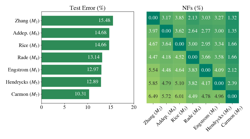
(b) Regression of accuracy, measured with NF rates.

Figure 2: Regression of robustness and accuracy for $M_{1},\ldots,M_{7}$ [21, 22, 23, 24, 25, 26, 27]. (a) Left: Robust error (%) of each model, sorted in descending order. Right: RNFs (%) attained when replacing old models (in rows) with new ones (in columns). (b) Left: Test error (%) of each model, sorted in descending order. Right: NFs (%) attained when replacing old models (in rows) with new ones (in columns). Values in the upper (lower) triangular matrices evaluate regression when the new model has better (worse) average robustness/accuracy than the old model.

Performance Metrics. We consider four relevant metrics, evaluated on $2,000$ test samples, to assess the performance of the given methods: (i) the test error, i.e., the percentage of misclassified (clean) test samples; (ii) the robust error, i.e., the percentage of misclassified adversarial examples; (iii) the fraction of negative flips (NFs, Eq. 1), to quantify the regression of accuracy; and (iv) the fraction of robustness negative flips (RNFs, Eq. 6), to evaluate the regression of robustness. To evaluate the robust error and the RNF rate, we optimize adversarial examples against each model using the AutoPGD attack [8] implemented in adversarial-library, with the Difference-of-Logit-Ratio (DLR) loss and $N=50$ iterations.

Hardware. All the experiments have been run on a workstation with an Intel^® Xeon^® Gold 5217 CPU with 32 cores (3.00 GHz), 192 GB of RAM, and two Nvidia^® RTX A6000 GPUs with 48 GB of memory each.

4.2 Evaluating Regression of Robustness

The first experiment presented here aims to empirically show that, once updated, machine-learning models are affected not only by a regression of accuracy, as shown in [1], but also by a regression of robustness. To show this novel phenomenon, as described in Sect. 4.1, we first rank the models $M_{1},...,M_{7}$ from the least to the most robust, based on the robust error evaluated on the $2,000$ test samples perturbed with AutoPGD. The models, along with their robust errors, are reported in order in 2(a) (left). Then, assuming a naïve update strategy that just replaces the old model with the new one, without performing any fine-tuning of the latter, we evaluate regression of robustness for all possible model pairs, as shown in 2(a) (right). Each cell of this matrix reports the regression of robustness (i.e., the fraction of RNFs) induced by the new model (reported in the corresponding column) when replacing the old one (reported in the corresponding row). The upper (lower) triangular matrix represents the cases in which the new model has better (lower) average robust error than the old one. The diagonal corresponds to replacing the model with itself, and thus no regression is observed. Even in the ideal case in which machine-learning models are updated with more robust ones (i.e., in the upper triangular matrix), we observe an RNF rate ranging from roughly $2\%$ to $6\%$. This implies that an increment in average robustness does not guarantee that previously-ineffective adversarial examples are still correctly classified.

We perform the same analysis on $M_{1},\ldots,M_{7}$ to quantify also their regression of accuracy. We thus re-order the models according to their reported test errors, as shown in 2(b) (left). We then consider again all the possible model pairs to simulate different model updates, and report the NFs corresponding to each naïve model update (i.e., by replacement) in 2(b) (right). Not surprisingly, all updates induce a regression of accuracy, even when the new models are more accurate than the old ones (i.e., in the upper triangular matrix), as also already shown by Yan et al. [1].

We can thus conclude that while updating machine-learning models may be beneficial to improve their average accuracy or robustness, this practice may induce a significant regression of both metrics when evaluated sample-wise.

TABLE I: Results for PCT, PCAT, and RCAT on the $10$ model updates with the highest RNF rates. In each update, denoted with ($M_{i},M_{j}$), the baseline model $M_{i}$ is replaced with $M_{j}$ using the naïve (replacement) strategy, or by fine-tuning $M_{j}$ with PCT, PCAT, and RCAT. For each update, we evaluate the test error, NFs, robust error, and RNFs (in %), and highlight in bold the method that achieves the best tradeoff between NFs and RNFs, i.e., the lowest value of their sum.

		Test Error	NFs	Robust Error	RNFs
(1) ($M_{3},M_{5}$)	baseline	14.66	-	41.55	-
	naïve	12.89	3.34	40.65	6.30
	PCT	6.77	1.20	66.10	26.10
	PCAT	9.80	2.10	47.55	10.95
	RCAT	11.25	2.30	40.45	6.00
(2) ($M_{4},M_{5}$)	baseline	13.14	-	40.90	-
	naïve	12.89	3.58	40.65	5.45
	PCT	6.16	1.02	72.95	32.35
	PCAT	8.69	1.65	47.20	9.60
	RCAT	10.82	1.76	41.55	5.60
(3) ($M_{1},M_{5}$)	baseline	12.97	-	44.15	-
	naïve	12.89	4.09	40.65	5.40
	PCT	8.01	1.88	55.70	14.40
	PCAT	9.34	2.26	47.90	8.80
	RCAT	10.75	2.52	40.50	4.55
(4) ($M_{3},M_{4}$)	baseline	14.66	-	41.55	-
	naïve	13.14	3.00	40.90	5.35
	PCT	8.48	1.37	51.30	12.45
	PCAT	9.99	1.72	44.90	7.80
	RCAT	11.04	1.68	40.90	4.60
(5) ($M_{2},M_{5}$)	baseline	15.48	-	44.05	-
	naïve	12.89	3.27	40.65	5.25
	PCT	5.35	1.12	84.05	40.35
	PCAT	8.81	1.65	47.00	8.35
	RCAT	11.81	2.27	40.45	4.85
(6) ($M_{2},M_{3}$)	baseline	15.48	-	44.05	-
	naïve	14.66	3.85	41.55	5.15
	PCT	10.59	1.76	46.90	7.70
	PCAT	14.53	2.41	42.10	3.15
	RCAT	14.25	3.29	41.90	5.05
(7) ($M_{5},M_{7}$)	baseline	12.89	-	40.65	-
	naïve	10.31	2.39	36.70	4.95
	PCT	6.47	1.21	40.90	7.55
	PCAT	7.55	1.73	38.85	6.75
	RCAT	8.30	1.45	36.50	4.65
(8) ($M_{3},M_{7}$)	baseline	14.66	-	41.55	-
	naïve	10.31	1.66	36.70	4.15
	PCT	7.40	0.97	41.10	6.25
	PCAT	8.74	1.24	39.00	4.75
	RCAT	8.80	1.21	37.55	4.35
(9) ($M_{6},M_{7}$)	baseline	14.68	-	39.45	-
	naïve	10.31	1.35	36.70	4.00
	PCT	7.16	1.06	42.75	8.25
	PCAT	7.93	1.34	40.15	6.95
	RCAT	8.92	1.10	37.80	5.00
(10) ($M_{1},M_{7}$)	baseline	12.97	-	44.15	-
	naïve	10.31	2.12	36.70	3.25
	PCT	8.01	1.22	41.50	4.30
	PCAT	9.31	1.33	40.95	3.70
	RCAT	8.41	1.11	37.15	2.80

4.3 Reducing Regression in Robust Image Classifiers

After having quantified the non-negligible impact of RNFs in model updates, we show here how RCAT can tackle this issue, outperforming the competing model update strategies of PCT and PCAT. To this end, we first select suitable model pairs that enable simulating updates in which the new model improves both accuracy and robustness w.r.t. the old one. This amounts to considering only $14$ model pairs (out of the overall $42$). Among these $14$ cases, we exclude $4$ model pairs exhibiting an RNF rate lower than $3\%$, which results in retaining the $10$ cases with the highest RNFs listed in Table I. Let us also recall that, when using the naïve update strategy, we just replace the old model $M_{i}$ with the new model $M_{j}$, and measure the corresponding NFs and RNFs. When using PCT, PCAT, and RCAT, we initialize the new model to be fine-tuned with $M_{j}$. Finally, for RCAT, we set $f^{\rm src}=M_{j}$.

Results for Model Updates. From the results in Table I, it is clear that RCAT provides a better trade-off between the reduction of NFs and that of RNFs w.r.t. the competing approaches in almost all cases. RCAT indeed achieves lower values of the sum of NFs and RNFs, while PCT and PCAT mostly reduce NFs by improving accuracy at the expense of compromising robustness. More specifically, PCT almost always entirely compromises robustness, as it is not designed to preserve it after update. A paradigmatic example can be found in row 5 of Table I, where PCT recovers almost 10% of test error w.r.t. the naïve strategy, lowering the NFs down to  1%, but increasing the robust error by  43%, with obvious consequences for the RNF rate that increases by  35%.

Measuring Performance Improvements ($\Delta$-metrics). To better highlight the differences among PCT, PCAT, and RCAT, for each update ($M_{i}$, $M_{j}$), we compute their performance improvements w.r.t. the baseline naïve strategy using these four additional metrics, referred to as $\Delta$-metrics in the following:

• $\Delta$ Test Error (%), i.e., the difference between the Test Error obtained by replacing $M_{i}$ with $M_{j}$ (naïve strategy) and that obtained using PCT, PCAT, or RCAT;

• $\Delta$ Robust Error (%), i.e., the difference between the Robust Error obtained by the naïve strategy and that obtained using PCT, PCAT, or RCAT;

• $\Delta$ NFs (%), i.e., the difference between the NF rate obtained by the naïve strategy and that obtained using PCT, PCAT, or RCAT; and

• $\Delta$ RNFs (%), i.e., the difference between the RNF rate obtained by the naïve strategy and that obtained using PCT, PCAT, or RCAT.

Accordingly, positive values of the $\Delta$-metrics represent an improvement w.r.t. naïve model replacement, i.e., a reduction of the test error, the robust error, NFs, and RNFs.

Analysis with $\Delta$-metrics. The results are reported in Fig. 3 and in Table II, along with the mean values of the $\Delta$-metrics, averaged on the model updates listed in Table I. From this analysis, the trends followed by PCT, PCAT, and RCAT become clearer: (i) PCT provides the largest improvement of accuracy (+4.62% on average) and reduction of NFs (+1.58% on average), at the expense of compromising adversarial robustness (-15.14% on average) and RNFs (-11.05% on average); (ii) PCAT works slightly better, but it still tends to improve accuracy (+2.59% on average) without retaining robustness (-4.38% on average), thereby improving NFs (+1.12% on average) and worsening RNFs (-2.16% on average); and (iii) RCAT finds a better accuracy-robustness trade-off than the competing approaches. In particular, it only slightly improves accuracy (+1.62% on average) and NFs (+1% on average), without affecting robustness (only -0.29% on average) and improving RNFs (+0.18% on average).

To summarize, performing model updates that retain high accuracy and robustness with low regression of both metrics is challenging. PCT and PCAT tend to recover accuracy but lose robustness. RCAT finds a better accuracy-robustness trade-off, providing a smaller improvement in accuracy and preserving robustness and, at the same time, minimizing the sum of NFs and RNFs, thereby effectively reducing both regression of accuracy and robustness.

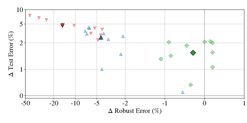
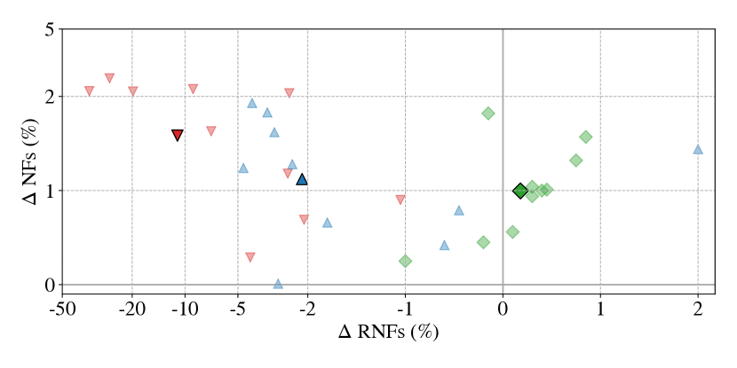
Figure 3: Performance improvements ($\Delta$-metrics) for each model update, when comparing naïve model replacement with PCT, PCAT, and RCAT. Positive values represent improvements w.r.t. naïve updates. Left: this plot shows $\Delta$ Test Error vs $\Delta$ Robust Error, highlighting the trade-off between accuracy and robustness of each method. Right: this plot shows $\Delta$ NFs vs $\Delta$ RNFs, highlighting the trade-off between reducing NFs and RNFs of each method. For each method, we report the individual model update values (transparent points) from Table I, and the corresponding average (opaque point) from Table II.

TABLE II: Mean values of the $\Delta$-metrics, averaged on all model updates shown in Table I. Positive values mean better results, i.e., lower test/robust error and NF/RNF rate w.r.t. to replacing the old model with the new one (naïve updates).

	$\Delta$ Test Error	$\Delta$ NFs	$\Delta$ Robust Error	$\Delta$ RNFs
PCT	+4.62	+1.58	-15.14	-11.05
PCAT	+2.59	+1.12	-4.38	-2.16
RCAT	+1.62	+1.00	-0.29	+0.18

5 Related Work

We discuss here methodologies that are related to our work. Continual Learning. Our work has ties to the research field of continual learning (CL) [29, 30], which aims to continuously re-train machine-learning models to deal with new classes, tasks, and domains, while only slightly adapting the initial architecture. It has however been shown that such continuous updates render CL techniques sensitive to catastrophic forgetting [31, 32], i.e., to forget previously-learned classes, tasks, or domains, while retaining good performance only on more recent data. Several techniques have been proposed to mitigate this issue, including: replay methods [33, 34], which replay representative samples from past data while re-training models on subsequent tasks; regularization terms [35, 36], which promote solutions with similar weights to those of the given model; and parameter isolation [37, 38], which separates weights attributed to the different task to be learned. However, as also explained in [1], we argue that quantifying the regression of models is not strictly connected to CL, as we are neither considering the inclusion of new tasks to learn nor the adaptation to the evolution of the data distribution. Furthermore, we do not restrict our update policy to maintain the same architecture, but we permit its replacement with a better one in terms of both accuracy and robustness.

Backward Compatibility. Our methodology can be included among the so-called backward-compatible [39, 40, 41] learning approaches, which focus on providing updates of machine learning models that can interchangeably replace previous versions without suffering loss in accuracy. This can be achieved by: (i) learning an invariant representation for newer and past data [41]; using different weights when predicting specific samples [42]; and (iii) estimating which samples should be re-evaluated as their labels might be incorrect. However, differently from RCAT, all these techniques only focus on accuracy, ignoring the side-effects on the regression of robustness, as the dramatic drop of performance we have observed when using PCT.

6 Conclusions and Future Work

Modern machine-learning systems demand frequent model updates to improve their average performance. To this end, more powerful architectures and additional data are often exploited in such systems to update the current models. However, it has been shown that model updates can induce a perceived regression of accuracy in the end users, as the new model may commit mistakes that the previous one did not make. The corresponding samples misclassified by the new model are referred to as negative flips (NFs). In this work, we show that NFs are not the sole regression that machine-learning models can face. Model updates can indeed cause also a significant regression of adversarial robustness. This means that, even if the average robustness of the updated model is higher, some adversarial examples that were ineffective against the previous model can become effective against the new one. We refer to these samples as robustness negative flips (RNFs). To address this issue, we propose a novel algorithm named RCAT, based on adversarial training, and theoretically show that our methodology provides a statistically-consistent estimator, without affecting the usual convergence rate of $O(\nicefrac{{1}}{{\sqrt{n}}})$. We empirically show the existence of RNF while updating robust image classification models, and compare the performance of our RCAT approach with the adversarially-robust version of PCT, namely PCAT. The results highlight that RCAT better handles the regression of robustness, by reducing the number of RNF and keeping almost the same performance as the previous model.

However, our methodology does not completely prevent the regression of robustness, but only mitigates it. Thus, as future research directions, we plan to improve the proposed approach by studying the effect of different loss functions and regularizers. Furthermore, while we only consider image classification in this work, we envision the presence of RNF also in other domains where machine-learning models require frequent updates, such as malware and spam detection. We plan to extend RCAT accordingly, to tackle the complexity of these non-trivial application domains. To conclude, we firmly believe that this first work can set up a novel line of research, which will educate practitioners to evaluate and mitigate the different types of regression that might be faced when dealing with machine-learning model updates.

Daniele Angioni is a Ph.D. candidate of the Italian National PhD Programme in Artificial Intelligence, working at the PRA Lab of the University of Cagliari, Italy. He received his B.Sc. degree in Electrical, Electronic and Computer Engineering in 2019, and his thesis was awarded with the second prize in the 15th edition of the Italian competition Premio Tesi Clusit “Innovare la sicurezza delle informazioni”. In 2021 he received his M.Sc. degree in Electronic Engineering with honors. His research addresses machine learning security in the real world, including attacks on image classifiers and malware detectors, and the mitigation of vulnerabilities introduced by model updates.

Luca Demetrio is Assistant Professor at the University of Genoa. He received his bachelor, master and Ph.D. degree at the University of Genova in 2015, 2017 and 2021. He is currently studying the security of Windows malware detectors implemented with Machine Learning techniques, and he is first author of papers published in top-tier journals (ACM TOPS, IEEE TIFS). He is part of the development team of SecML, and the maintainer of SecML Malware, a Python library for creating adversarial Windows malware.

Maura Pintor is an Assistant Professor at the University of Cagliari, Italy. She received her MSc degree in Telecommunications Engineering (with honors) in 2018, and her PhD in Electronic and Computer Engineering (with honors) in 2022 from the University of Cagliari. Her research interests include adversarial machine learning and explainability methods, with applications in cybersecurity. Her PhD work, summarized in the thesis “Towards Debugging and Improving Adversarial Robustness Evaluations,” provides a framework for optimizing and debugging adversarial attacks. She serves as a PC member for NeurIPS, ICLR, and ICCV, and as a reviewer for several top-tier journals (IEEE TIFS, IEEE TDSC, IEEE-TNNLS, IEEE TIP, ACM TOPS).

Luca Oneto received his BSc and MSc in Electronic Engineering at the University of Genoa, in 2008 and 2010, and he received his PhD from the same university in 2014. In 2018 he was co-funder of the spin-off ZenaByte s.r.l. In 2019 he became Associate Professor in Computer Science at University of Pisa, and currently is Associate Professor in Computer Engineering at University of Genoa. He has been involved in several H2020 projects (S2RJU, ICT, DS) and he has been awarded with the Amazon AWS Machine Learning and Somalvico (best Italian young AI researcher) Awards. His main topic of research is the Statistical Learning Theory with particular focus on the theoretical aspects of the problems of (Semi) Supervised Model Selection and Error Estimation.

Davide Anguita received the “Laurea” degree in Electronic Engineering and a Ph.D. degree in Computer Science and Electronic Engineering from the University of Genoa, Genoa, Italy, in 1989 and 1993, respectively. After working as a Research Associate at the International Computer Science Institute, Berkeley, CA, on special-purpose processors for neurocomputing, he returned to the University of Genoa. He is currently Full Professor of Computer Engineering with the Department of Informatics, BioEngineering, Robotics, and Systems Engineering (DIBRIS). His current research focuses on the theory and application of kernel methods and artificial neural networks.

Battista Biggio (MSc 2006, PhD 2010) is an Associate Professor of Computer Engineering at the University of Cagliari, Italy. He has provided pioneering contributions in machine learning security, playing a leading role in this field. His seminal paper “Poisoning Attacks against Support Vector Machines” won the prestigious 2022 ICML Test of Time Award. He has managed more than 10 research projects, and regularly serves as a PC member for ICML and USENIX Sec., and as Area Chair for NeurIPS. He chaired IAPR TC1 (2016-2020), and served as Associate Editor for IEEE TNNLS, IEEE CIM, and Elsevier Pattern Recognition. He is now Associate Editor-in-Chief for PRJ. He is Senior Member of IEEE and ACM, and Member of IAPR and ELLIS.

Fabio Roli is a Full Professor of Computer Engineering at the University of Genova and the University of Cagliari, Italy, and Founding Director of the Pattern Recognition and Applications laboratory at the University of Cagliari. He has been doing research on the design of pattern recognition and machine learning systems for thirty years. He has provided seminal contributions to the fields of multiple classifier systems and adversarial machine learning, and he has played a leading role in the establishment and advancement of these research themes. He has been appointed Fellow of the IEEE and Fellow of the International Association for Pattern Recognition. He is a recipient of the Pierre Devijver Award for his contributions to statistical pattern recognition.

References

- [1] S. Yan, Y. Xiong, K. Kundu, S. Yang, S. Deng, M. Wang, W. Xia, and S. Soatto, “Positive-congruent training: Towards regression-free model updates,” in IEEE/CVF Conference on Computer Vision and Pattern Recognition, 2021.
- [2] F. Croce, M. Andriushchenko, V. Sehwag, E. Debenedetti, N. Flammarion, M. Chiang, P. Mittal, and M. Hein, “Robustbench: a standardized adversarial robustness benchmark,” in Neural Information Processing Systems, 2021.
- [3] A. Madry, A. Makelov, L. Schmidt, D. Tsipras, and A. Vladu, “Towards deep learning models resistant to adversarial attacks,” in Int’l Conference on Learning Representations, 2018.
- [4] B. Biggio, I. Corona, D. Maiorca, B. Nelson, N. Šrndić, P. Laskov, G. Giacinto, and F. Roli, “Evasion attacks against machine learning at test time,” in European Conference on Machine Learning and Knowledge Discovery in Databases, 2013.
- [5] I. Goodfellow, J. Shlens, and C. Szegedy, “Explaining and harnessing adversarial examples,” in ICLR, 2015.
- [6] N. Carlini, A. Athalye, N. Papernot, W. Brendel, J. Rauber, D. Tsipras, I. Goodfellow, A. Madry, and A. Kurakin, “On evaluating adversarial robustness,” ArXiv e-prints, vol. 1902.06705, 2019.
- [7] M. Pintor, F. Roli, W. Brendel, and B. Biggio, “Fast minimum-norm adversarial attacks through adaptive norm constraints,” in Neural Information Processing Systems, 2021.
- [8] F. Croce and M. Hein, “Reliable evaluation of adversarial robustness with an ensemble of diverse parameter-free attacks,” in ICML, 2020.
- [9] T. Hastie, R. Tibshirani, J. H. Friedman, and J. H. Friedman, The elements of statistical learning: data mining, inference, and prediction. Springer, 2009, vol. 2.
- [10] L. Oneto, S. Ridella, and D. Anguita, “The benefits of adversarial defense in generalization,” Neurocomputing, vol. 505, pp. 125–141, 2022.
- [11] I. Goodfellow, Y. Bengio, and A. Courville, Deep learning. MIT press, 2016.
- [12] C. C. Aggarwal, Neural networks and deep learning. Springer, 2018.
- [13] N. Srivastava, G. Hinton, A. Krizhevsky, I. Sutskever, and R. Salakhutdinov, “Dropout: a simple way to prevent neural networks from overfitting,” The journal of machine learning research, vol. 15, no. 1, pp. 1929–1958, 2014.
- [14] P. L. Bartlett and S. Mendelson, “Rademacher and gaussian complexities: Risk bounds and structural results,” Journal of Machine Learning Research, vol. 3, pp. 463–482, 2002.
- [15] D. Yin, R. Kannan, and P. Bartlett, “Rademacher complexity for adversarially robust generalization,” in Int’l conference on machine learning, 2019.
- [16] R. Bassily, K. Nissim, A. Smith, T. Steinke, U. Stemmer, and J. Ullman, “Algorithmic stability for adaptive data analysis,” in ACM symposium on Theory of Computing, 2016.
- [17] D. Russo and J. Zou, “Controlling bias in adaptive data analysis using information theory,” in Int’l Conference on Artificial Intelligence and Statistics, 2016.
- [18] S. Shalev-Shwartz and S. Ben-David, Understanding machine learning: From theory to algorithms. Cambridge university press, 2014.
- [19] K. Ito and B. Jin, Inverse problems: Tikhonov theory and algorithms. World Scientific, 2014.
- [20] L. Oneto, S. Ridella, and D. Anguita, “Tikhonov, ivanov and morozov regularization for support vector machine learning,” Machine Learning, vol. 103, pp. 103–136, 2016.
- [21] L. Engstrom, A. Ilyas, H. Salman, S. Santurkar, and D. Tsipras, “Robustness (python library),” 2019. [Online]. Available: https://github.com/MadryLab/robustness
- [22] J. Zhang, X. Xu, B. Han, G. Niu, L. Cui, M. Sugiyama, and M. Kankanhalli, “Attacks which do not kill training make adversarial learning stronger,” in International conference on machine learning. PMLR, 2020, pp. 11 278–11 287.
- [23] L. Rice, E. Wong, and Z. Kolter, “Overfitting in adversarially robust deep learning,” in International Conference on Machine Learning. PMLR, 2020, pp. 8093–8104.
- [24] R. Rade and S.-M. Moosavi-Dezfooli, “Helper-based adversarial training: Reducing excessive margin to achieve a better accuracy vs. robustness trade-off,” in ICML Workshop on Adversarial Machine Learning, 2021.
- [25] D. Hendrycks, K. Lee, and M. Mazeika, “Using pre-training can improve model robustness and uncertainty,” in 36th ICML, ser. PMLR, K. Chaudhuri and R. Salakhutdinov, Eds., vol. 97, 2019, pp. 2712–2721.
- [26] S. Addepalli, S. Jain, G. Sriramanan, and R. Venkatesh Babu, “Scaling adversarial training to large perturbation bounds,” in European Conference on Computer Vision. Springer, 2022, pp. 301–316.
- [27] Y. Carmon, A. Raghunathan, L. Schmidt, J. C. Duchi, and P. Liang, “Unlabeled data improves adversarial robustness,” in NeurIPS, H. M. Wallach, H. Larochelle, A. Beygelzimer, F. d’Alché-Buc, E. B. Fox, and R. Garnett, Eds., 2019, pp. 11 190–11 201.
- [28] E. Wong, L. Rice, and J. Z. Kolter, “Fast is better than free: Revisiting adversarial training,” in ICLR, 2020.
- [29] Z. Chen and B. Liu, Lifelong machine learning. Springer, 2018, vol. 1.
- [30] M. De Lange, R. Aljundi, M. Masana, S. Parisot, X. Jia, A. Leonardis, G. Slabaugh, and T. Tuytelaars, “A continual learning survey: Defying forgetting in classification tasks,” IEEE transactions on pattern analysis and machine intelligence, vol. 44, no. 7, pp. 3366–3385, 2021.
- [31] J. Kirkpatrick, R. Pascanu, N. Rabinowitz, J. Veness, G. Desjardins, A. A. Rusu, K. Milan, J. Quan, T. Ramalho, A. Grabska-Barwinska et al., “Overcoming catastrophic forgetting in neural networks,” National Academy of Sciences, vol. 114, no. 13, pp. 3521–3526, 2017.
- [32] M. Toneva, A. Sordoni, R. T. des Combes, A. Trischler, Y. Bengio, and G. J. Gordon, “An empirical study of example forgetting during deep neural network learning,” in ICLR, 2019.
- [33] H. Ahn, J. Kwak, S. Lim, H. Bang, H. Kim, and T. Moon, “Ss-il: Separated softmax for incremental learning,” in Proc. IEEE/CVF Int’l Conf. on computer vision, 2021, pp. 844–853.
- [34] A. Chaudhry, M. Rohrbach, M. Elhoseiny, T. Ajanthan, P. Dokania, P. Torr, and M. Ranzato, “Continual learning with tiny episodic memories,” in Workshop on Multi-Task and Lifelong Reinforcement Learning, 2019.
- [35] H. Ahn, S. Cha, D. Lee, and T. Moon, “Uncertainty-based continual learning with adaptive regularization,” in NeurIPS, 2019, pp. 4394–4404.
- [36] S. Wang, X. Li, J. Sun, and Z. Xu, “Training networks in null space of feature covariance for continual learning,” in Proc. IEEE/CVF Conf. on Computer Vision and Pattern Recognition, 2021, pp. 184–193.
- [37] A. Mallya and S. Lazebnik, “Packnet: Adding multiple tasks to a single network by iterative pruning,” in Proc. IEEE Conf. on Computer Vision and Pattern Recognition, 2018, pp. 7765–7773.
- [38] J. Serra, D. Suris, M. Miron, and A. Karatzoglou, “Overcoming catastrophic forgetting with hard attention to the task,” in ICML. PMLR, 2018, pp. 4548–4557.
- [39] Y. Zhao, Y. Shen, Y. Xiong, S. Yang, W. Xia, Z. Tu, B. Shiele, and S. Soatto, “Elodi: Ensemble logit difference inhibition for positive-congruent training,” arXiv preprint arXiv:2205.06265, 2022.
- [40] F. Träuble, J. von Kügelgen, M. Kleindessner, F. Locatello, B. Schölkopf, and P. V. Gehler, “Backward-compatible prediction updates: A probabilistic approach,” in NeurIPS, 2021, pp. 116–128.
- [41] Y. Shen, Y. Xiong, W. Xia, and S. Soatto, “Towards backward-compatible representation learning,” in Proceedings of the IEEE/CVF Conference on Computer Vision and Pattern Recognition, 2020, pp. 6368–6377.
- [42] M. Srivastava, B. Nushi, E. Kamar, S. Shah, and E. Horvitz, “An empirical analysis of backward compatibility in machine learning systems,” in Proceedings of the 26th ACM SIGKDD International Conference on Knowledge Discovery & Data Mining, 2020, pp. 3272–3280.