Prediction of the SYM-H Index Using a Bayesian Deep Learning Method with Uncertainty Quantification

Abstract

We propose a novel deep learning framework, named SYMHnet, which employs a graph neural network and a bidirectional long short-term memory network to cooperatively learn patterns from solar wind and interplanetary magnetic field parameters for short-term forecasts of the SYM-H index based on 1-minute and 5-minute resolution data. SYMHnet takes, as input, the time series of the parameters’ values provided by NASA’s Space Science Data Coordinated Archive and predicts, as output, the SYM-H index value at time point $t$ + $w$ hours for a given time point $t$ where $w$ is 1 or 2. By incorporating Bayesian inference into the learning framework, SYMHnet can quantify both aleatoric (data) uncertainty and epistemic (model) uncertainty when predicting future SYM-H indices. Experimental results show that SYMHnet works well at quiet time and storm time, for both 1-minute and 5-minute resolution data. The results also show that SYMHnet generally performs better than related machine learning methods. For example, SYMHnet achieves a forecast skill score (FSS) of 0.343 compared to the FSS of 0.074 of a recent gradient boosting machine (GBM) method when predicting SYM-H indices (1 hour in advance) in a large storm (SYM-H = $-393$ nT) using 5-minute resolution data. When predicting the SYM-H indices (2 hours in advance) in the large storm, SYMHnet achieves an FSS of 0.553 compared to the FSS of 0.087 of the GBM method. In addition, SYMHnet can provide results for both data and model uncertainty quantification, whereas the related methods cannot.

Space Weather

Institute for Space Weather Sciences, New Jersey Institute of Technology, Newark, NJ 07102, USA

Department of Computer Science, New Jersey Institute of Technology, Newark, NJ 07102, USA

College of Applied Computer Sciences, King Saud University, Riyadh 11451, Saudi Arabia

Center for Solar-Terrestrial Research, New Jersey Institute of Technology, Newark, NJ 07102, USA

Big Bear Solar Observatory, New Jersey Institute of Technology, Big Bear City, CA 92314, USA

Space Science and Applications, Los Alamos National Laboratory, Los Alamos, NM 87545, USA

Department of Physics, Canakkale Onsekiz Mart University, 17110 Canakkale, Turkey

Harvard-Smithsonian Center for Astrophysics, 60 Garden Street, Cambridge, MA 02138, USA

Jason T. L. Wangwangj@njit.edu

SYMHnet is a novel deep learning method for making short-term predictions of the SYM-H index (1 or 2 hours in advance).

With Bayesian inference, SYMHnet can quantify both aleatoric (data) and epistemic (model) uncertainties in making its prediction.

SYMHnet generally performs better than related machine learning methods for SYM-H forecasting.

Plain Language Summary

In the past several years, machine learning and its subfield, deep learning, have attracted considerable interest. Computer vision, natural language processing, and social network analysis make extensive use of machine learning algorithms. Recent applications of these algorithms include the prediction of solar flares and the forecasting of geomagnetic indices. In this paper, we propose an innovative machine learning method that utilizes a graph neural network and a bidirectional long short-term memory network to cooperatively learn patterns from solar wind and interplanetary magnetic field parameters to provide short-term predictions of the SYM-H index. In addition, we present techniques for quantifying both data and model uncertainties in the output of the proposed method.

1 Introduction

Geomagnetic activities and events are known to have a substantial impact on the Earth. They can damage and affect technological systems such as telecommunication networks, power transmission systems, and spacecraft [Ayala Solares . (2016), Jordanova . (2020)]. These activities are massive and scale on orders of magnitude [Newell . (2007)]. It may take a few days to recover from the damage, depending on its severity. These activities and events cannot be ignored regardless of whether they are in regions at high, medium, or low latitudes [Carter . (2016), Gaunt  Coetzee (2007), Moldwin  Tsu (2016), Tozzi . (2019), Viljanen . (2014)]. Therefore, several activity indices have been developed to measure the intensity of the geomagnetic effects. These indices characterize the magnitude of the disturbance over time. Modeling and forecasting these geomagnetic indices have become a crucial area of study in space weather research.

Some indices, such as Kp, describe the overall level of geomagnetic activity while others, such as the disturbance storm time (Dst) index [Woodroffe . (2016)], describe a specific area of geomagnetic activity. The Dst index has been used to classify a storm based on its intensity  [Bala  Reiff (2012), Gruet . (2018), Lazzús . (2017), Lu . (2016), Xu . (2023)]. The storm is intense when Dst is less than $-100$ nT, moderate when Dst is between $-100$ nT and $-50$ nT, and weak when Dst is greater than $-50$ nT [Gruet . (2018), Nuraeni . (2022)]. Another important index is the symmetric H-component index (SYM-H), which is used to represent the longitudinally symmetric disturbance of the intensity of the ring current during geomagnetic storms. The SYM-H index is the one-minute version of the DST index, obtained by data from more stations [Rangarajan (1989), Siciliano . (2021), Vichare . (2019), Wanliss  Showalter (2006)]. On the other hand, ASY-H (the asymmetric geomagnetic disturbance of the horizontal component) is quantified as the longitudinally asymmetric part of the geomagnetic disturbance field at low latitude to midlatitude. In addition, there are other indices that can be used to measure the activity of the storm as described in Mayaud1980.

A lot of efforts have been devoted to developing strategies to alleviate the geomagnetic effects on technologies and humans, but it is almost impossible to offer complete protection from the effects [Siciliano . (2021)]. Some of these strategies are to predict the occurrence and intensity of geomagnetic storms to offer some level of mitigation of their damaging effects. For example, BurtonEaAl1975 established an empirical connection between interplanetary circumstances and Dst using a linear forecasting model. Temerin2002Dst developed an explicit model to predict Dst on the basis of solar wind data for the years 1995–1999, by finding functions and values of free parameters that minimize the root square error (RMS error) between their model and the measured Dst. Wang2033DiffEqu used differential equation models to examine the effect of the dynamic pressure of the solar wind on the decay and injection of the ring current. YurchyshynBz2004SpWea22001Y proposed that the hourly averaged magnitude of the Bz component of the magnetic field in interplanetary ejecta is correlated with the speed of the CME, which may open a way to predict the Dst index using CME parameters. AyalaEffectOfMagneticOnEarth performed predictions of global magnetic disturbance in near-Earth space in a case study for the Kp index using Nonlinear AutoRegressive with eXogenous (NARX) models. Due to the intrinsic complex response of the circumterrestrial environment to changes in the interplanetary medium, these simple models were unable to properly and fully depict the evolution of the solar wind-magnetosphere-ionosphere system [Consolini  Chang (2001), Klimas . (1996), Siciliano . (2021)]. To surpass the limitations of simple models and acquire the complex response of the magnetosphere, researchers resorted to more advanced models such as artificial neural networks (ANNs).

The use of ANNs focused on the prediction of the Dst and Kp indices. Lundstedt-1994 constructed the first Dst prediction model employing a time-delay ANN with solar wind parameters as input variables. LazzusDstSwarmOptizmizedRNN2017 created a particle swarm optimization method to train ANN connection weights to improve the accuracy of the prediction of the Dst index. Bala2012KpForecasting combined ANNs and physical models with solar wind and interplanetary magnetic field parameters such as velocity, interplanetary magnetic field (IMF) magnitude, and clock angle. ChandorkarGaussianDST2017 used Gaussian processes (GP) to build an autoregressive model to predict the Dst index 1 hour in advance based on the past solar wind velocity, the IMF component $B_{z}$, and the values of the Dst index. This method generated a predictive distribution rather than a single prediction point. However, the mean values of the estimations are not as accurate as those generated by ANNs. GCS2018 overcame the poor performance of GP and constructed a Dst index estimation model by merging GP with a long short-term memory (LSTM) network to obtain more accurate results. More recently, DstBayesianXU20233882 developed a new GP regression model that performed better than related distance correlation learning methods [Lu . (2016)] in forecasting the Dst index during intense geomagnetic storms. Raster2013ComparisonDst1MinuteSpWea..11..187R compared the effectiveness of 30 Dst forecast models and found that none of the models performed consistently the best for all events.

Relatively few researchers have focused on the prediction of SYM-H. This happens probably because of the high temporal resolution of 1 minute for the SYM-H index, which gives rise to a more difficult problem in estimating SYM-H due to its highly oscillating nature [Siciliano . (2021)]. However, some SYM-H index prediction techniques have been reported in the literature. Caiangeo-28-381-2010 presented the first 5-minute average estimates of the SYM-H index throughout large storms between 1998 and 2006 using a NARX neural network with IMF and solar wind data. SYMHForecastStPatric2019JSWSC…9A..12B predicted both the SYM-H and ASY-H indices for solar cycle 24 by employing the NARX neural network in a similar way. Both SYMHForecastStPatric2019JSWSC…9A..12B and Caiangeo-28-381-2010 used the IMF magnitude ($B$), $B_{y}$ and $B_{z}$ components, as well as the density and velocity of the solar wind as input data for their models. SYMHForecasting2021ComparisonLSTMCNN provided a comprehensive examination of two well-known deep learning models, namely long short-term memory (LSTM) and a convolutional neural network (CNN), with an average temporal resolution of 5 minutes for the estimation of SYM-H index values (1 hour in advance). The authors used the IMF component $B_{z}$, squared values of the magnitude of the IMF $B$ and the $B_{y}$ component, measured at L1 by the ACE satellite in GSM coordinates. 2021ColladoSMYH_ASYH_CNN_LSTMForecasting created neural network models for the SYM-H and ASY-H predictions by combining CNN and LSTM. The authors considered 42 geomagnetic storms between 1998 and 2018 for model training, validation, and testing purposes. 2022XGBoostSYMHbyIong developed a model using gradient boosting machines to predict the SYM-H index (1 and 2 hours in advance) with a temporal resolution of 5 minutes.

In this paper, we present a new method, named SYMHnet, that utilizes cooperative learning of a graph neural network (GNN) and a bidirectional long short-term memory (BiLSTM) network with Bayesian inference to conduct short-term (1 or 2 hours in advance) predictions of the SYM-H index for solar cycles 23 and 24. We consider temporal resolutions of 1 minute and 5 minutes, respectively, for the SYM-H index. To our knowledge, this is the first time that 1-minute resolution data have been used to predict the SYM-H index. Furthermore, our method can quantify both model and data uncertainties when producing prediction results, whereas related machine learning methods cannot.

The remainder of this paper is organized as follows. Section 2 describes the data, including the solar wind and IMF parameters, as well as geomagnetic storms, used in this study. Section 3 presents the methodology, explaining the SYMHnet framework, its architecture, and the uncertainty quantification algorithm. Section 4 evaluates the performance of SYMHnet on 1-minute and 5-minute resolution data. We also report the experimental results obtained by comparing SYMHnet with related machine learning methods on 5-minute resolution data. Section 5 presents a discussion and concludes the paper.

2 Database

In training and evaluating SYMHnet, we built a database that combines the solar wind and IMF parameters with the geomagnetic storms studied in this paper. This database contains 42 storms selected from the past two solar cycles (#23 and #24). The storms occurred between 1998 and 2018.

2.1 Solar Wind and IMF Parameters

We consider seven solar wind, IMF, and derived parameters: IMF magnitude ($B$), $B_{y}$ and $B_{z}$ components, flow speed, proton density, electric field and flow pressure. These parameters have been used in related studies [Bhaskar  Vichare (2019), Cai . (2010), Denton . (2016), Iong . (2022)]. The parameters’ values along with the SYM-H index values are collected from the NASA Space Science Data Coordinated Archive available at https://nssdc.gsfc.nasa.gov [King  Papitashvili (2005)]. Data are collected with 1- and 5-minute resolutions.

2.2 Geomagnetic Storms

We work with the same storms as those considered in previous studies [Collado-Villaverde . (2021), Iong . (2022), Siciliano . (2021)]. Table 1 lists the storms used to train SYMHnet. Table 2 lists the storms used to validate SYMHnet. Table 3 lists the storms used to test SYMHnet. The training set, validation set, and test set are disjoint. Thus, SYMHnet can make predictions on storms that it has never seen during training. Note that each storm period listed in Tables 1, 2, and 3 contains both quiet time and storm time, as indicated by the maximum SYM-H and minimum SYM-H values in the period.

Table 1: Storms Used to Train SYMHnet

Storm #	Start Date	End Date	Min SYM-H (nT)	Max SYM-H (nT)
1	02/14/1998	02/22/1998	$-119$	12
2	08/02/1998	08/08/1998	$-168$	25
3	09/19/1998	09/29/1998	$-213$	8
4	02/16/1999	02/24/1999	$-127$	28
5	10/15/1999	10/25/1999	$-218$	42
6	07/09/2000	07/19/2000	$-335$	76
7	08/06/2000	08/16/2000	$-235$	10
8	09/15/2000	09/25/2000	$-196$	43
9	11/01/2000	11/15/2000	$-174$	43
10	03/14/2001	03/24/2001	$-165$	22
11	04/06/2001	04/16/2001	$-275$	32
12	10/17/2001	10/22/2001	$-210$	37
13	10/31/2001	11/10/2001	$-313$	43
14	05/17/2002	05/27/2002	$-113$	101
15	11/15/2003	11/25/2003	$-488$	10
16	07/20/2004	07/30/2004	$-208$	32
17	05/10/2005	05/20/2005	$-302$	64
18	04/09/2006	04/19/2006	$-110$	24
19	10/09/2006	12/19/2006	$-206$	39
20	03/01/2012	03/11/2012	$-149$	49

Table 2: Storms Used to Validate SYMHnet

Storm #	Start Date	End Date	Min SYM-H (nT)	Max SYM-H (nT)
21	04/28/1998	05/08/1998	$-268$	50
22	09/19/1999	09/26/1999	$-160$	64
23	10/25/2003	11/03/2003	$-427$	33
24	06/18/2015	06/28/2015	$-207$	77
25	09/01/2017	09/11/2017	$-144$	54

Table 3: Storms Used to Test SYMHnet

Storm #	Start Date	End Date	Min SYM-H (nT)	Max SYM-H (nT)
26	06/22/1998	06/30/1998	$-120$	39
27	11/02/1998	11/12/1998	$-179$	19
28	01/09/1999	01/18/1999	$-111$	9
29	04/13/1999	04/19/1999	$-122$	63
30	01/16/2000	01/26/2000	$-101$	21
31	04/02/2000	04/12/2000	$-315$	16
32	05/19/2000	05/28/2000	$-159$	47
33	03/26/2001	04/04/2001	$-434$	109
34	05/26/2003	06/06/2003	$-162$	10
35	07/08/2003	07/18/2003	$-125$	23
36	01/18/2004	01/27/2004	$-137$	41
37	11/04/2004	11/14/2004	$-393$	92
38	09/10/2012	10/05/2012	$-138$	18
39	05/28/2013	06/04/2013	$-134$	37
40	06/26/2013	07/04/2013	$-110$	19
41	03/11/2015	03/21/2015	$-233$	62
42	08/22/2018	09/03/2018	$-205$	26

3 Methodology

Machine learning (ML) and its subfield, deep learning (DL) [Goodfellow . (2016)], have been used extensively in the space weather community for predicting solar flares [Abduallah . (2021), Huang . (2018), Liu . (2019)], flare precursors [Chen . (2019)], coronal mass ejections [Alobaid . (2022), Liu . (2020)], solar energetic particles [Abduallah . (2022), Laurenza . (2009), Lavasa . (2021), Núñez (2011), Stumpo . (2021)], and geomagnetic indices [Amata . (2008), Bala  Reiff (2012), Bhaskar  Vichare (2019), Collado-Villaverde . (2021), Gruet . (2018), Lazzús . (2017), Pallocchia . (2006), Siciliano . (2021)]. Different from the existing methods, SYMHnet combines a graph neural network (GNN) and a bidirectional long short-term memory (BiLSTM) network to jointly learn patterns from input data. GNN learns the relationships among the parameter values in the input data, while BiLSTM captures the temporal dynamics of the input data. As our experimental results show later, this combined learning framework works well and generally performs better than related machine learning methods for SYM-H index forecasting.

3.1 Parameter Graph

We construct an undirected unweighted fully connected graph (FCG) for the solar wind, the IMF and the derived parameters considered in this study, where each node represents a parameter and there is an edge between every two nodes. Because the parameter values are time series, we obtain a time series of parameter graphs where the topologies of the graphs are the same, but the node values vary as time goes on. For example, Figure 1 shows three parameter graphs constructed at time points $t$, $t$ + 1, $t$ + 2, respectively, with a resolution of 1 minute to predict the SYM-H index 1 hour in advance. In Figure 1, the leftmost graph at $t$ contains the values of the seven parameters, represented by seven nodes or circles, at the time point $t$. The FCG symbol in the center indicates that this is a fully connected graph in which every two nodes are connected by an edge. (For simplicity, only a portion of the edges are shown in the figure.) Furthermore, the graph contains a node that represents the value of the SYM-H index at the time point $t$ + 1 hour. During training, this SYM-H index value is used as the label for the graph. The GNN in SYMHnet will learn the relationships among the parameters’ values and the relationships between the parameters’ values and the label. If we want to predict the SYM-H index 2 hours in advance, then the label will be the SYM-H index value at the time point $t$ + 2 hours.

The middle graph at $t$ + 1 in Figure 1 contains the values of the seven parameters at the time point $t$ + 1 minute. In addition, this graph contains the SYM-H index value at the time point ($t$ + 1 minute) + 1 hour, which is the label for this graph. If we want to predict the SYM-H index 2 hours in advance, then the label will be the SYM-H index value at the time point ($t$ + 1 minute) + 2 hours.

The rightmost graph at $t$ + 2 in Figure 1 contains the values of the seven parameters at the time point $t$ + 2 minutes. Additionally, this graph contains the SYM-H index value at the time point ($t$ + 2 minutes) + 1 hour, which is the label for this graph. If we want to predict the SYM-H index 2 hours in advance, then the label will be the SYM-H index value at the time point ($t$ + 2 minutes) + 2 hours.

During testing/prediction, given the values of the seven parameters at a time point $t^{\prime}$ (without a label), SYMHnet will predict the label, which is the SYM-H index value at the time point $t^{\prime}$ + 1 hour (for 1-hour ahead predictions) or the SYM-H index value at the time point $t^{\prime}$ + 2 hours (for 2-hour ahead predictions), as detailed in Section 3.2.

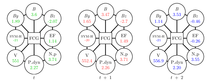
Figure 1: Illustration of the parameter graphs constructed at time points $t$, $t$ + 1, $t$ + 2, respectively with a resolution of 1 minute for predicting the SYM-H index 1 hour in advance. Each graph contains seven parameters: IMF magnitude ($B$), $B_{y}$ component, $B_{z}$ component, electric field (EF), proton density (N_p), flow pressure (P_dyn), and flow speed (V). The colored values in the graphs represent the parameters’ values that change as time goes on, while the topologies of the graphs remain the same. The value in the SYM-H node in a graph is the label of the graph. The FCG symbol in a graph indicates that the graph is fully connected.

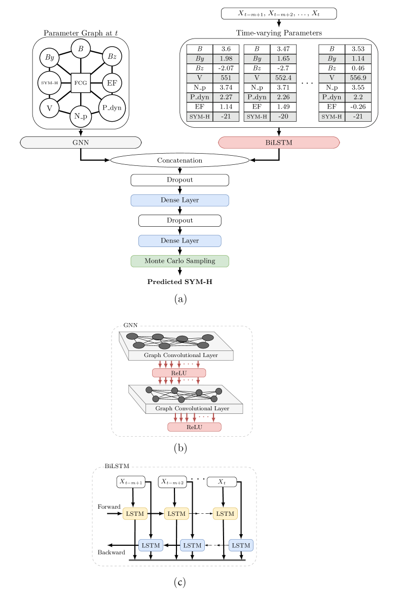
Figure 2: The SYMHnet framework: (a) the overall architecture of SYMHnet, (b) the architecture of its GNN component, and (c) the architecture of its BiLSTM component. The input parameter graph is for illustration; the actual graph in the implementation is a fully connected graph (FCG). B = IMF magnitude (B), By = By component, Bz = Bz component, EF = Electric field, N_p = Proton density, P_dyn = Flow pressure, and V = Flow speed.

3.2 The SYMHnet Framework

Figure 2 illustrates the SYMHnet framework. During training, we feed the input data sample at each time point in turn to SYMHnet. The input data sample at the time point $t$ consists of the parameter graph $G_{t}$ constructed at $t$ and a sequence of $m$ records $X_{t-m+1}$, $X_{t-m+2}$, $\ldots$, $X_{t}$ where $X_{i}$, $t-m+1\leq i\leq t$, represents the record collected at the time point $i$. $X_{i}$ contains the seven values of the solar wind and IMF parameters along with the SYM-H index value at the time point $i$. Including previous SYM-H index values in the input to predict future SYM-H indices improves prediction accuracy [Iong . (2022)]. The number of records, $m$, in the input is set to 10 which was determined by our experiments. When m $<$ 10, BiLSTM cannot effectively capture the temporal patterns in the data. When m $>$ 10, it causes additional overhead for larger sequence sizes without improving prediction accuracy. The label of the graph $G_{t}$ is used as the label of the input data sample at the time point $t$.

The parameter graph $G_{t}$ is sent to SYMHnet’s GNN component [Panagopoulos . (2021)] while the sequence of $m$ records, $X_{t-m+1}$, $X_{t-m+2}$, $\ldots$, $X_{t}$, is sent to SYMHnet’s BiLSTM component [Abduallah . (2022)]. The GNN, illustrated in Figure 2(b), contains a graph convolutional layer followed by a rectified linear unit (ReLU), which is followed by another graph convolutional layer and ReLU. The BiLSTM network, illustrated in Figure 2(c), is composed of two LSTM layers [Hochreiter  Schmidhuber (1997)] with opposite directions when processing the data. This architecture allows the BiLSTM network to use one LSTM layer to read the sequence from the end to the beginning, denoted as forward, and the other LSTM layer to read the sequence from the beginning to the end, denoted as backward. GNN is good for learning the correlations between nodes (parameters) in a graph [Panagopoulos . (2021)] while BiLSTM is suitable for learning the temporal patterns in time series [Abduallah . (2022), Siami-Namini . (2019)]. SYMHnet combines the learned parameter correlations and temporal patterns into a joint pattern, which is then passed to two dropout and dense layers.

A dropout layer provides a mechanism to randomly drop a percentage of neurons to avoid over-fitting on the training data so that the SYMHnet model can generalize to unseen test data. It also enables the Monte Carlo (MC) sampling method described in Section 3.3 because the internal structure of the network is slightly different each time neurons are dropped [Gal  Ghahramani (2016), Jiang . (2021)]. Each neuron in a dense layer connects to every neuron in the preceding layer [Goodfellow . (2016)]. The dense layer helps to change the dimensionality of the output of the preceding layer so that the SYMHnet model can easily define the relationship between the values of the data on which the model works. In this way, we better train our model, and the model learns things more effectively. Table 4 summarizes the details of the model architecture.

During testing/prediction, we feed an unlabeled test data sample to SYMHnet where the test data sample is the same as the training data sample, except that the test data sample does not have a label. The trained SYMHnet model will predict the label based on the input test data sample. SYMHnet uses the MC dropout sampling method described in Section 3.3 to produce, for a test data sample, a predicted SYM-H index value accompanied by results of aleatoric uncertainty and epistemic uncertainty.

Table 4: Architecture Details of SYMHnet

Component	Parameter	Value
Forward LSTM	Number of LSTM units	400
Backward LSTM	Number of LSTM units	400
	Activation function	ReLU
GNN	Number of nodes	8
	Number of edges	56
	Activation function	ReLU
	Number of graph convolutional layers	2
Dense layer	Number of neurons	200

3.3 Uncertainty Quantification

Quantification of uncertainty is essential for the reproducibility and validation of a model [Volodina  Challenor (2021)]. Uncertainty quantification with deep learning has been used in computer vision [Kendall  Gal (2017)], space weather [Gruet . (2018)], and solar physics [Jiang . (2021)]. There are two types of uncertainty: aleatoric and epistemic. Aleatoric uncertainty captures the inherent randomness of data, hence also referred to as data uncertainty. Epistemic uncertainty occurs due to the inexact weight calculations in a neural network and is also known as model uncertainty.

In incorporating Bayesian inference into SYMHnet, our goal is to find the posterior distribution over the weights of the network, $W$, given the observed training data, $X$, and the labels $Y$, that is, $P(W|X,Y)$. The posterior distribution is intractable [Jiang . (2021)], and one has to approximate the weight distribution [Denker  LeCun (1990)]. We use variational inference as suggested by Graves_VaritionalNIPS2011_7eb3c8be to learn the variational distribution on the weights of the network, $q(W)$, by minimizing the Kullback–Leibler (KL) divergence of $q(W)$ and $P(W|X,Y)$.

Training a network with dropout [Srivastava . (2014)] is equivalent to a variational approximation on the network [Gal  Ghahramani (2016)]. Furthermore, minimizing the loss function of cross-entropy (CE) [Goodfellow . (2016)] can have the same effect as minimizing the KL divergence term. Minimizing CE loss in classification problems is equivalent to minimizing mean squared error (MSE) loss in regression problems [Hung . (2020), Kline  Berardi (2005)]. Therefore, we use the MSE loss function and the root mean squared propagation (RMSProp) optimizer with a learning rate of 0.0002 to train SYMHnet. Table 5 summarizes the hyperparameters and their values used by SYMHnet. We use $\hat{q}(W)$ to represent the optimized weight distribution.

During testing/prediction, SYMHnet uses the MC dropout sampling method [Gal  Ghahramani (2016)] to quantify uncertainty. Specifically, we process the test data $K$ times to generate $K$ MC samples where $K$ is set to 100. We have experimented with different $K$ values. Using a $K$ value of less than 100 does not generate enough samples; the produced uncertainty ranges are too large to be useful. Using a $K$ value of larger than 100 increases computation time, while the model performance remains the same. As a consequence, we set $K$ to 100 to process the test data 100 times. Each time, a set of weights is randomly drawn from $\hat{q}(W)$. We obtain the mean and variance for the $K$ samples. The mean is the anticipated SYM-H value. According to HaodiFibri2021, we split the variance into aleatoric and epistemic uncertainties.

Table 5: Hyperparameter Values Used by SYMHnet

Parameter	Value
Dropout rate	0.5
Batch size	1024
Epochs	50
Optimizer	RMSProp
Learning rate	0.0002
Loss function	MSE

4 Experiments and Results

4.1 Performance Metrics

To assess the prediction accuracy of SYMHnet and compare it with related machine learning models, we adopt the following metrics: root mean square error (RMSE), forecast skill score (FSS) and R-squared (R²). These metrics have been used in the forecasting of geomagnetic indices and are recommended in the literature [Camporeale (2019), Iong . (2022), Liemohn . (2018)]. Our experiments were carried out by feeding time series data samples from the training storms in Table 1 (training set) to train a model. We then used the time series data samples from the validation storms in Table 2 (validation set) to validate the model and optimize its hyperparameters. Finally, we used the trained model to predict the SYM-H index values of the time series data samples from the test storms in Table 3 (test set).

RMSE measures the difference between prediction and ground truth for each test data sample. It is calculated as follows:

$$\mbox{RMSE}=\sqrt{\frac{1}{n}\sum_{i=1}^{n}({y_{i}}-\hat{y_{i}})^{2}},$$ (1)

where $n$ is the number of test data samples in a test storm in Table 3, and $\hat{y_{i}}$ ($y_{i}$, respectively) represents the predicted SYM-H index value (observed SYM-H index value, respectively) at the time point $i$ in the test storm. The smaller the RMSE, the more accurate the model.

FSS is calculated using the prediction provided by the Burton equation [O’Brien  McPherron (2000a)] as a baseline and is defined as follows [Iong . (2022), Murphy (1988)]:

$$\mbox{FSS}=1-\frac{\frac{1}{n}\sum_{i=1}^{n}({y_{i}}-\hat{y_{i}})^{2}}{\frac{1}{n}\sum_{i=1}^{n}({y_{i}}-y_{i}^{b})^{2}}$$ (2)

where $y_{i}^{b}$ represents the prediction provided by the Burton equation at the time point $i$ in the test storm. The FSS value between 0 and 1 indicates that the model is better than the baseline, while the negative FSS value indicates that the model is worse than the baseline [Iong . (2022)].

R² determines the amount of variance of the observed data explained by the predicted data. It is calculated as follows:

$$\mbox{ R\textsuperscript{2} }=1-\frac{\sum_{i=1}^{n}({y_{i}}-\hat{y_{i}})^{2}}{\sum_{i=1}^{n}({y_{i}}-\bar{y})^{2}},$$ (3)

where $\bar{y}$ is the mean of the observed SYM-H index values for the test data samples in the test storm. The larger the R², the more accurate the model.

For each metric, the mean and standard deviation of the metric values for all test storms in the test set (Table 3) are calculated and recorded.

4.2 Results Based on 1-Minute Resolution Data

In this section, we present experimental results based on the 1-minute resolution data in our database. First, we conducted an ablation study to analyze and assess the components of SYMHnet. Then we performed case studies on a moderately large storm (storm #36 with SYM-H = $-137$ nT) and a very large storm (storm #37 with SYM-H = $-393$ nT) in the test set shown in Table 3 where both storms were previously investigated by 2022XGBoostSYMHbyIong. It should be noted that the work of 2022XGBoostSYMHbyIong was based on 5-minute resolution data. To our knowledge, no previous method used 1-minute resolution data to predict the SYM-H index.

4.2.1 Ablation Study with 1-Minute Resolution Data

We considered three variants of SYMHnet: SYMHnet-B, SYMHnet-G and SYMHnet-BG. SYMHnet-B represents the subnetwork of SYMHnet with the BiLSTM component removed. SYMHnet-G represents the subnetwork of SYMHnet with the GNN component removed. SYMHnet-BG represents the subnetwork of SYMHnet with both the BiLSTM and GNN components removed. Thus, SYMHnet-BG simply contains the dense layers in SYMHnet, which amounts to a simple multilayer perceptron network. When conducting the ablation study, we turned off the uncertainty quantification mechanism.

Table 6 presents the average values for RMSE, FSS, and R² (with standard deviations enclosed in parentheses) obtained by the four models: SYMHnet, SYMHnet-B, SYMHnet-G and SYMHnet-BG, based on the 1-minute resolution data in our database. The best metric values are highlighted in boldface. It can be seen from Table 6 that SYMHnet outperforms its three variants. SYMHnet-B is the second best among the four models, implying that a GNN is effective in solving time series regression problems [Bloemheuvel . (2022)]. SYHMnet-G, which contains a BiLSTM network but no GNN, does not perform well. This finding is consistent with those in 2021ColladoSMYH_ASYH_CNN_LSTMForecasting, who showed that LSTM performed worse than a combination of LSTM and CNN in SYM-H forecasting. Finally, SYMHnet-BG is the worst among the four models. This happens because SYMHnet-BG loses the advantages offered by GNN and BiLSTM networks.

Table 6: Results of the Ablation Study Based on 1-Minute Resolution Data

Metric	Hour-ahead	SYMHnet	SYMHnet-B	SYMHnet-G	SYMHnet-BG
RMSE	1	3.002 (2.169)	3.210 (2.319)	4.194 (3.030)	5.348 (2.957)
	2	3.171 (2.201)	3.432 (2.382)	4.369 (3.033)	5.623 (3.066)
FSS	1	0.668 (0.131)	0.563 (0.003)	0.007 (0.012)	$-0.644$ (0.015)
	2	0.760 (0.089)	0.387 (0.031)	$-0.367$ (0.016)	$-0.731$ (0.031)
R2	1	0.993 (0.003)	0.913 (0.001)	0.789 (0.001)	0.602 (0.001)
	2	0.993 (0.003)	0.908 (0.002)	0.776 (0.002)	0.594 (0.002)

4.2.2 Case Studies with 1-Minute Resolution Data

Here we conducted case studies by using SYMHnet to predict the SYM-H index values in storms #36 and #37 given in Table 3 based on the 1-minute resolution data in our database. Additional case studies on other storms can be found in Appendix A. The period of storm #36 started on 18 January 2004 and ended on 27 January 2004, with a minimum SYM-H value of $-137$ nT and a maximum SYM-H value of 41 nT during the period. The period of storm #37 started on 4 November 2004 and ended on 14 November 2004, with a minimum SYM-H value of $-393$ nT and a maximum SYM-H value of 92 nT during the period. Figure 3 shows the predictions and measured error of the SYMHnet model in storm #36 and storm #37 respectively. In the figure, each point on a yellow dashed line represents the prediction made at the corresponding time $x$ on the X-axis. For 1-hour ahead (2-hour ahead, respectively) predictions, the point/prediction at time $x$ is produced based on the solar wind/IMF parameters at time $x$ – 1 hour ($x$ – 2 hours, respectively). There is a lag of 1 hour (for 1-hour ahead predictions) or 2 hours (for 2-hour ahead predictions) as in previous studies [Collado-Villaverde . (2021), Iong . (2022)]. It can be seen from Figure 3 that the SYMHnet model works well at both quiet time and storm time. The measured error ranges between $-15$ nT and 23 nT for storm #36 and between $-50$ nT and 34 nT for storm #37. The more intense the storm, the larger the measured error.

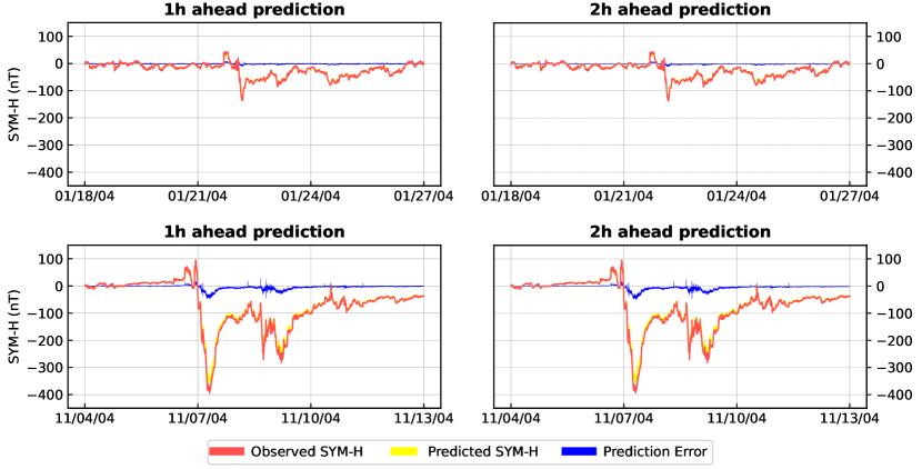
Figure 3: Predictions for storm #36 (top) and storm #37 (bottom) made by the SYMHnet model based on 1-minute resolution data. The red line represents the observed SYM-H values, the yellow dashed line represents the model’s predictions, and the blue line represents the prediction error. Both quiet time and storm time are shown in the figure.

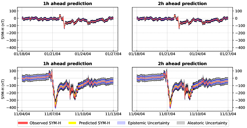
Figure 4: Uncertainty quantification results produced by the SYMHnet model in storm #36 (top) and storm #37 (bottom) based on 1-minute resolution data. The red line represents the observed SYM-H values, the yellow dashed line represents the model’s predictions, the light-blue region shows epistemic uncertainty (model uncertainty), and the light-gray region shows aleatoric uncertainty (data uncertainty). Both quiet time and storm time are shown in the figure.

Figure 4 presents uncertainty quantification results produced by SYMHnet in storm #36 and storm #37, respectively, based on the 1-minute resolution data in our database. In the figure, the red line represents the observed values of the SYM-H index, and the yellow dashed line represents the predicted values of the SYM-H index. The light-blue region shows the epistemic uncertainty (model uncertainty) and the light-gray region shows the aleatoric uncertainty (data uncertainty) of the predicted outcome. It can be seen in Figure 4 that the yellow dashed line (predicted values) is reasonably close to the red line (observed values), again demonstrating the good performance of SYMHnet. The light-blue region is tinier than the light-gray region, indicating that the model uncertainty is lower than the data uncertainty. This is due to the fact that the uncertainty in the predicted outcome is primarily caused by the noise in the input test data, not by the SYMHnet model.

4.3 Results Based on 5-Minute Resolution Data

SYMHnet can be easily modified to process 5-minute resolution data. As described in Section 3.2, the input data sample at the time point $t$ is composed of the parameter graph $G_{t}$ and a sequence of $m$ records. The difference is that the cadence of the $m$ records here is 5-minute rather than 1-minute. Furthermore, the labels of the parameter graphs $G_{t}$, $G_{t+5}$, $G_{t+10}$ are the SYM-H index values at the time points $t$ + $w$ hour, ($t$ + 5 minutes) + $w$ hour, ($t$ + 10 minutes) + $w$ hour, respectively, for $w$-hour ahead predictions where $w$ is 1 or 2.

In the following, we present experimental results based on the 5-minute resolution data in our database. As in Section 4.2, we conducted an ablation study, this time using the 5-minute resolution data. We then performed case studies on storms #36 and #37. Finally, we compared SYMHnet with related machine learning methods, all of which utilized the 5-minute resolution data in our database. Since the related methods cannot quantify uncertainty, we turned off the uncertainty quantification mechanism in SYMHnet while conducting the comparative study.

4.3.1 Ablation Study with 5-Minute Resolution Data

Table 7 presents the average values for RMSE, FSS and R² (with standard deviations enclosed in parentheses) obtained by the four models: SYMHnet, SYMHnet-B, SYMHnet-G and SYMHnet-BG, based on the 5-minute resolution data in our database. The best metric values are highlighted in boldface. It can be seen from Table 7 that SYMHnet is again the best among the four models for the 5-minute resolution data, a finding consistent with that in Table 6 for the 1-minute resolution data.

Table 7: Results of the Ablation Study Based on 5-Minute Resolution Data

Metric	Hour-ahead	SYMHnet	SYMHnet-B	SYMHnet-G	SYMHnet-BG
RMSE	1	5.914 (2.169)	6.324 (2.319)	8.262 (2.834)	10.537 (2.958)
	2	6.481 (2.201)	8.646 (2.636)	13.021 (3.315)	14.165 (3.194)
FSS	1	0.484 (0.195)	0.407 (0.087)	0.005 (0.012)	$-0.465$ (0.023)
	2	0.593 (0.096)	0.302 (0.048)	$-0.286$ (0.035)	$-0.570$ (0.042)
R2	1	0.993 (0.003)	0.912 (0.003)	0.789 (0.004)	0.601 (0.005)
	2	0.989 (0.003)	0.905 (0.003)	0.773 (0.004)	0.592 (0.005)

4.3.2 Case Studies with 5-Minute Resolution Data

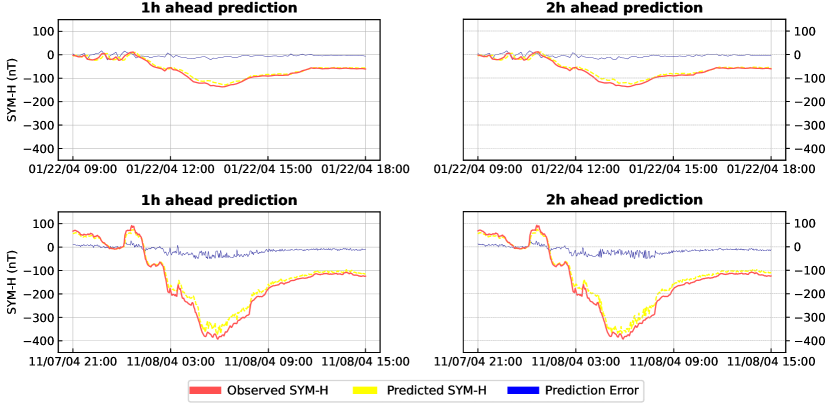
Figure 5: Predictions for storm #36 (top) and storm #37 (bottom) made by the SYMHnet model based on 5-minute resolution data. The red line represents the observed SYM-H values, the yellow dashed line represents the model’s predictions, and the blue line represents the prediction error. Only the peak storm time is shown in the figure.

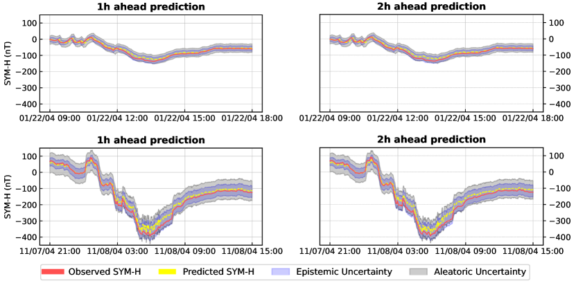
Figure 6: Uncertainty quantification results produced by the SYMHnet model in storm #36 (top) and storm #37 (bottom) based on 5-minute resolution data. The red line represents the observed SYM-H values, the yellow dashed line represents the model’s predictions, the light-blue region shows epistemic uncertainty (model uncertainty), and the light-gray region shows aleatoric uncertainty (data uncertainty). Only the peak storm time is shown in the figure.

Figure 5 shows the predictions and measured error of SYMHnet in storms #36 and #37, respectively, and Figure 6 presents the uncertainty quantification results produced by SYMHnet in these storms respectively, based on the 5-minute resolution data in our database. Unlike Figures 3 and 4, in which both quiet time and storm time are shown, Figures 5 and 6 focus on the peak storm time. In Figure 5, the measured error ranges between $-24$ nT and 25 nT for storm #36 and between $-52$ nT and 36 nT for storm #37. These results indicate that SYMHnet can properly forecast the SYM-H index even in the most intense storm period.

In Figure 6, the red line represents the observed values of the SYM-H and the yellow dashed line represents the predicted values of the SYM-H. The light-blue area shows the epistemic uncertainty (model uncertainty) and the light-gray area shows the aleatoric uncertainty (data uncertainty) of the predicted outcome. It can be seen from Figure 6 that the red line representing the observed SYM-H values is within the uncertainty interval, indicating SYMHnet’s predicted values together with the uncertainty values well cover the observed values. The overall findings here are similar to those from the 1-minute resolution data shown in Figure 4.

4.3.3 Comparative Study with 5-Minute Resolution Data

Several researchers performed SYM-H forecasting using machine learning and the 5-minute resolution data. 2021ColladoSMYH_ASYH_CNN_LSTMForecasting combined long short-term memory (LSTM) and a convolutional neural network (CNN), referred to as the LCNN method, to forecast the SYM-H index (1 and 2 hours in advance). 2022XGBoostSYMHbyIong utilized gradient boosting machines, referred to as the GBM method, to forecast the SYM-H index (also 1 and 2 hours in advance). SYMHForecasting2021ComparisonLSTMCNN compared LSTM and CNN for the prediction of the SYM-H index (only 1 hour in advance). Although the methods including ours use slightly different data samples, these methods are all developed to predict the SYM-H index values in the same set of storms. The purpose of this comparative study is to compare the prediction results/accuracies of, rather than specific models/data samples in, these methods. This comparison methodology has commonly been used in SYM-H forecasting [Collado-Villaverde . (2021), Iong . (2022), Siciliano . (2021)]. Since the related methods cannot predict uncertainties, we turned off the uncertainty quantification component in SYMHnet while carrying out the comparative study. The Burton equation [O’Brien  McPherron (2000a)], used as the baseline, is also included. The performance metric values of each method for each test storm in the test set (Table 3) are calculated. The best metric values are highlighted in boldface.

Tables 8 and 9 compare the RMSE results of these methods for 1-hour and 2-hour ahead SYM-H predictions, respectively, based on the RMSE values available in the related studies [Collado-Villaverde . (2021), Iong . (2022), O’Brien  McPherron (2000a), Siciliano . (2021)]. Tables 10 and 11 compare the FSS results of these methods for 1-hour and 2-hour ahead SYM-H predictions, respectively, based on the FSS values available in the related studies [Collado-Villaverde . (2021), Iong . (2022), Siciliano . (2021)]. Table 12 compares the R² results of these methods for 1-hour ahead and 2-hour ahead SYM-H predictions, respectively, on the same test storms. 2022XGBoostSYMHbyIong did not provide R² results, and hence the GBM method was excluded from Table 12. These tables show that SYMHnet performs better than the related methods for all except two test storms (#28 and/or #40), demonstrating the good performance and feasibility of our tool for SYM-H forecasting.

Table 8: RMSEs for 1-hr Ahead Prediction from the Comparative Study Including SYMHnet, LCNN [Collado-Villaverde . (2021)], GBM [Iong . (2022)], LSTM and CNN [Siciliano . (2021)], and Burton Equation [O’Brien  McPherron (2000a)]

	1-h ahead prediction (RMSE)
Storm #	SYMHnet	LCNN	GBM	LSTM	CNN	Burton
26	3.977	6.630	5.863	6.700	7.200	6.839
27	7.682	8.913	7.729	8.900	10.500	7.955
28	4.599	5.858	4.281	5.400	5.600	5.967
29	5.058	6.683	5.833	7.200	7.700	6.511
30	2.213	5.200	4.927	5.600	6.500	4.614
31	7.923	8.584	8.277	10.700	9.600	8.838
32	3.969	7.259	6.841	8.300	8.200	9.487
33	11.366	13.340	14.492	16.300	19.100	16.630
34	5.259	10.034	10.190	11.300	12.400	10.888
35	5.406	7.693	7.154	8.500	8.800	7.918
36	5.618	9.525	8.512	8.700	10.500	9.082
37	10.320	15.184	14.548	17.500	17.300	15.713
38	3.368	4.080	3.886	4.200	4.600	4.572
39	5.670	6.431	5.901	5.700	6.800	6.663
40	5.752	4.673	4.976	5.500	5.900	5.371
41	5.871	7.882	7.558	9.000	9.400	8.358
42	3.900	5.669	5.030	5.900	6.300	5.549

Table 9: RMSEs for 2-hr Ahead Prediction from the Comparative Study Including SYMHnet, LCNN [Collado-Villaverde . (2021)], GBM [Iong . (2022)], and Burton Equation [O’Brien  McPherron (2000a)]

	2-h ahead prediction (RMSE)
Storm #	SYMHnet	LCNN	GBM	Burton
26	4.330	8.989	8.285	10.690
27	8.577	13.418	11.585	12.465
28	4.977	5.877	5.650	8.858
29	5.515	9.314	8.826	9.776
30	2.636	7.288	7.280	6.266
31	9.737	12.436	12.613	13.604
32	4.451	8.937	9.927	13.766
33	13.745	18.481	24.519	25.729
34	5.611	13.941	13.736	14.695
35	5.830	9.932	9.504	10.586
36	5.970	12.058	12.068	13.117
37	10.923	21.084	22.327	24.446
38	3.765	5.213	5.153	6.546
39	6.252	6.798	7.391	10.159
40	6.336	5.281	5.633	6.032
41	6.857	11.707	12.121	12.622
42	4.674	8.273	7.976	8.877

Table 10: FSSs for 1-hr Ahead Prediction from the Comparative Study Including SYMHnet, LCNN [Collado-Villaverde . (2021)], GBM [Iong . (2022)], LSTM and CNN [Siciliano . (2021)]

	1-h ahead prediction (FSS)
Storm #	SYMHnet	LCNN	GBM	LSTM	CNN
26	0.418	0.031	0.143	0.020	$-0.053$
27	0.034	$-0.120$	0.028	$-0.119$	$-0.320$
28	0.229	$-0.028$	0.249	0.095	0.062
29	0.223	$-0.026$	0.104	$-0.106$	$-0.183$
30	0.520	$-0.127$	$-0.068$	$-0.214$	$-0.409$
31	0.104	0.029	0.063	$-0.211$	$-0.086$
32	0.582	0.235	0.279	0.125	0.136
33	0.317	0.198	0.129	0.020	$-0.149$
34	0.517	0.078	0.064	$-0.038$	$-0.139$
35	0.317	0.028	0.096	$-0.074$	$-0.111$
36	0.381	$-0.049$	0.063	0.042	$-0.156$
37	0.343	0.034	0.074	$-0.114$	$-0.101$
38	0.263	0.108	0.150	0.081	$-0.006$
39	0.149	0.035	0.114	0.160	$-0.021$
40	$-0.071$	0.130	0.074	$-0.024$	$-0.098$
41	0.298	0.057	0.096	$-0.077$	$-0.125$
42	0.297	$-0.022$	0.094	$-0.063$	$-0.135$

Table 11: FSSs for 2-hr Ahead Prediction from the Comparative Study Including SYMHnet, LCNN [Collado-Villaverde . (2021)], and GBM [Iong . (2022)]

	2-h ahead prediction (FSS)
Storm #	SYMHnet	LCNN	GBM
26	0.595	0.159	0.225
27	0.312	$-0.076$	0.071
28	0.438	0.337	0.362
29	0.436	0.047	0.097
30	0.579	$-0.163$	$-0.162$
31	0.284	0.086	0.073
32	0.677	0.351	0.279
33	0.466	0.282	0.047
34	0.618	0.051	0.065
35	0.449	0.062	0.102
36	0.545	0.081	0.080
37	0.553	0.138	0.087
38	0.425	0.204	0.213
39	0.385	0.331	0.272
40	$-0.050$	0.125	0.066
41	0.457	0.072	0.040
42	0.473	0.068	0.101

Table 12: R²s for 1- and 2-hr Ahead Predictions from the Comparative Study Including SYMHnet, LCNN [Collado-Villaverde . (2021)], LSTM and CNN [Siciliano . (2021)]

	1-h ahead prediction (R2)				2-h ahead prediction (R2)
Storm #	SYMHnet	LCNN	LSTM	CNN	SYMHnet	LCNN
26	0.956	0.870	0.890	0.870	0.948	0.766
27	0.952	0.939	0.940	0.920	0.940	0.862
28	0.957	0.936	0.950	0.950	0.949	0.936
29	0.955	0.922	0.930	0.920	0.946	0.848
30	0.991	0.946	0.950	0.930	0.987	0.894
31	0.976	0.971	0.960	0.970	0.963	0.939
32	0.986	0.953	0.950	0.950	0.982	0.929
33	0.979	0.965	0.960	0.950	0.969	0.932
34	0.945	0.798	0.750	0.700	0.938	0.612
35	0.954	0.907	0.900	0.890	0.947	0.845
36	0.949	0.864	0.890	0.840	0.943	0.782
37	0.993	0.966	0.960	0.960	0.992	0.934
38	0.961	0.939	0.940	0.930	0.951	0.900
39	0.964	0.932	0.960	0.940	0.943	0.924
40	0.948	0.966	0.950	0.950	0.937	0.957
41	0.984	0.969	0.960	0.960	0.978	0.931
42	0.985	0.968	0.970	0.960	0.978	0.932

5 Discussion and Conclusion

Geomagnetic activities have a significant impact on Earth, which can cause damages to spacecraft, electrical power grids, and navigation systems. Geospace scientists use geomagnetic indices to measure and quantify the geomagnetic activities. The SYM-H index provides information about the response and behavior of the Earth’s magnetosphere during geomagnetic storms. Therefore, a lot of effort has been put into SYM-H forecasting. Previous work mainly focused on 5-minute resolution data and skipped 1-minute resolution data. The higher temporal resolution of the 1-minute resolution data poses a more difficult challenge to forecast due to its highly oscillating character. This oscillating behavior could make the data more noisy to a machine learning model. As a consequence, the model requires more iterations during training with a larger number of neurons in order to learn more features and patterns hidden in the data.

In our study, the SYMHnet model architectures for processing the 1-minute resolution data and 5-minute resolution data are the same, as shown in Figure 2. The configuration details and hyperparameter values of SYMHnet for processing the 5-minute resolution data are shown in Tables 4 and 5. When processing the 1-minute resolution data, the model is configured with a larger number of neurons in the dense layers, a higher percentage in the dropout layers, and a larger number of epochs during the training phase. This configuration is designed to combat the highly oscillating behavior of the 1-minute resolution data.

Results from our experiments demonstrated the good performance of SYMHnet at both quiet time and storm time. These results were obtained from a database of 42 storms that occurred between 1998 and 2018 during the past two solar cycles (#23 and #24). As done in previous studies [Collado-Villaverde . (2021), Iong . (2022), Siciliano . (2021)], 20 storms, listed in Table 1, were used for training, 5 storms, listed in Table 2, were used for validation, and 17 storms, listed in Table 3, were used for testing. Based on the tables, the 42 storms were distributed to 14 distinct years.

To avoid bias in drawing a conclusion from the above experiments, we conducted an additional experiment using 14-fold cross validation where the data was divided into 14 partitions or folds. Each fold corresponds to one year in which at least one storm occurred. The sequential order of the data in each fold was maintained. In each run, one fold was used for testing and the other 13 folds together were used for training. Thus, the training set and test set are disjoint, and the trained model can predict unseen SYM-H values in the test set. There were 14 folds and consequently 14 runs where the average performance metric values over the 14 runs were calculated. The results of the 14-fold cross validation were consistent with those reported in the paper. These results indicate that the SYMHnet tool can be used to predict future SYM-H index values without knowing whether a storm is going to start. When the predicted SYM-H value is less than a threshold (e.g., $-30$ nT), the tool detects the occurrence of a storm. Thus, we conclude that the proposed SYMHnet is a viable machine learning method for short-term, 1 or 2-hour ahead forecasts of the SYM-H index for both 1- and 5-minute resolution data.

Data Availability Statement

• The solar wind, IMF and derived parameters along with the SYM-H index data used in our study are publicly available from NASA’s Space Physics Data Facility at http://omniweb.gsfc.nasa.gov/ow.html.

• Details of SYMHnet can be found at https://doi.org/10.5281/zenodo.10602518.

Appendix A Additional Case Studies with 1-Minute Resolution Data

Figure 7 shows the predictions and measured error of SYMHnet in storms #28, #31, #33, #40, and #42, respectively, and Figure 8 presents the uncertainty quantification results produced by SYMHnet in these storms, respectively, based on the 1-minute resolution data in our database. The period of storm #28 started on 9 January 1999 and ended on 18 January 1999, with a minimum SYM-H value of $-111$ nT and a maximum SYM-H value of 9 nT. The period of storm #31 started on 2 April 2000 and ended on 12 April 2000, with a minimum SYM-H value of $-315$ nT and a maximum SYM-H value of 16 nT. The period of storm #33 stared on 26 March 2001 and ended on 4 April 2001, with a minimum SYM-H value of $-434$ nT and a maximum SYM-H value of 109 nT. The period of storm #40 started on 26 June 2013 and ended on 4 July 2013, with a minimum SYM-H value of $-110$ nT and a maximum SYM-H value of 19 nT. The period of storm #42 started on 22 August 2018 and ended on 3 September 2018, with a minimum SYM-H value of $-205$ nT and a maximum SYM-H value of 26 nT. In Figure 7, the measured error ranges between $-46$ nT and 7 nT for storm #28, between $-58$ nT and 2 nT for storm #31, between $-69$ nT and 32 nT for storm #33, between $-12$ nT and 4 nT for storm #40, and between $-26$ nT and 7 nT for storm #42. Generally, the more intense the storm, the larger the measured error. In Figure 8, we see that SYMHnet’s predicted values together with the uncertainty values well cover the observed values, a finding consistent with that in Figure 4.

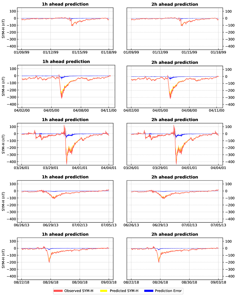
Figure 7: Predictions for storms (from top to bottom) #28 in January 1999, #31 in April 2000, #33 in March 2001, #40 in June 2013, and #42 in August 2018, made by the SYMHnet model based on 1-minute resolution data. The red line represents the observed SYM-H values, the yellow dashed line represents the model’s predictions, and the blue line represents the prediction error. Both quiet time and storm time are shown in the figure.

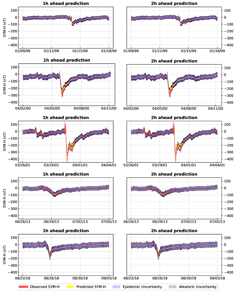
Figure 8: Uncertainty quantification results produced by the SYMHnet model in storms (from top to bottom) #28 in January 1999, #31 in April 2000, #33 in March 2001, #40 in June 2013, and #42 in August 2018, based on 1-minute resolution data. The red line represents the observed SYM-H values, the yellow dashed line represents the model’s predictions, the light-blue region shows epistemic uncertainty (model uncertainty), and the light-gray region shows aleatoric uncertainty (data uncertainty). Both quiet time and storm time are shown in the figure.

References

- Abduallah \BOthers. (\APACyear2022) \APACinsertmetastarAbduallahSEP2022{APACrefauthors}Abduallah, Y., Jordanova, V\BPBIK., Liu, H., Li, Q., Wang, J\BPBIT\BPBIL.\BCBL \BBA Wang, H. \APACrefYearMonthDay2022. \BBOQ\APACrefatitlePredicting Solar Energetic Particles Using SDO/HMI Vector Magnetic Data Products and a Bidirectional LSTM Network Predicting solar energetic particles using SDO/HMI vector magnetic data products and a bidirectional LSTM network.\BBCQ \APACjournalVolNumPagesThe Astrophysical Journal Supplement Series260116. {APACrefURL} https://doi.org/10.3847/1538-4365/ac5f56 \PrintBackRefs\CurrentBib
- Abduallah \BOthers. (\APACyear2021) \APACinsertmetastarMLaaS_RAA_Abduallah_2021{APACrefauthors}Abduallah, Y., Wang, J\BPBIT\BPBIL., Nie, Y., Liu, C.\BCBL \BBA Wang, H. \APACrefYearMonthDay2021. \BBOQ\APACrefatitleDeepSun: Machine-learning-as-a-service for solar flare prediction DeepSun: Machine-learning-as-a-service for solar flare prediction.\BBCQ \APACjournalVolNumPagesResearch in Astronomy and Astrophysics217160. {APACrefURL} https://doi.org/10.1088/1674-4527/21/7/160 \PrintBackRefs\CurrentBib
- Alobaid \BOthers. (\APACyear2022) \APACinsertmetastarKhalidCMEFronteirs2022{APACrefauthors}Alobaid, K\BPBIA., Abduallah, Y., Wang, J\BPBIT\BPBIL., Wang, H., Jiang, H., Xu, Y.\BDBLJing, J. \APACrefYearMonthDay2022. \BBOQ\APACrefatitlePredicting CME arrival time through data integration and ensemble learning Predicting CME arrival time through data integration and ensemble learning.\BBCQ \APACjournalVolNumPagesFrontiers in Astronomy and Space Sciences91013345. {APACrefURL} https://doi.org/10.3389/fspas.2022.1013345 \PrintBackRefs\CurrentBib
- Amata \BOthers. (\APACyear2008) \APACinsertmetastar2008JASTP..70..496A{APACrefauthors}Amata, E., Pallocchia, G., Consolini, G., Marcucci, M\BPBIF.\BCBL \BBA Bertello, I. \APACrefYearMonthDay2008. \BBOQ\APACrefatitleComparison between three algorithms for Dst predictions over the 2003-2005 period Comparison between three algorithms for Dst predictions over the 2003-2005 period.\BBCQ \APACjournalVolNumPagesJournal of Atmospheric and Solar-Terrestrial Physics702-4496-502. {APACrefURL} https://doi.org/10.1016/j.jastp.2007.08.041 \PrintBackRefs\CurrentBib
- Ayala Solares \BOthers. (\APACyear2016) \APACinsertmetastarAyalaEffectOfMagneticOnEarth{APACrefauthors}Ayala Solares, J\BPBIR., Wei, H\BHBIL., Boynton, R\BPBIJ., Walker, S\BPBIN.\BCBL \BBA Billings, S\BPBIA. \APACrefYearMonthDay2016. \BBOQ\APACrefatitleModeling and prediction of global magnetic disturbance in near-Earth space: A case study for Kp index using NARX models Modeling and prediction of global magnetic disturbance in near-Earth space: A case study for Kp index using NARX models.\BBCQ \APACjournalVolNumPagesSpace Weather1410899-916. {APACrefURL} https://doi.org/10.1002/2016SW001463 \PrintBackRefs\CurrentBib
- Bala \BBA Reiff (\APACyear2012) \APACinsertmetastarBala2012KpForecasting{APACrefauthors}Bala, R.\BCBT \BBA Reiff, P. \APACrefYearMonthDay2012. \BBOQ\APACrefatitleImprovements in short-term forecasting of geomagnetic activity Improvements in short-term forecasting of geomagnetic activity.\BBCQ \APACjournalVolNumPagesSpace Weather106. {APACrefURL} https://doi.org/10.1029/2012SW000779 \PrintBackRefs\CurrentBib
- Bhaskar \BBA Vichare (\APACyear2019) \APACinsertmetastarSYMHForecastStPatric2019JSWSC…9A..12B{APACrefauthors}Bhaskar, A.\BCBT \BBA Vichare, G. \APACrefYearMonthDay2019. \BBOQ\APACrefatitleForecasting of SYMH and ASYH indices for geomagnetic storms of solar cycle 24 including St. Patrick’s day, 2015 storm using NARX neural network Forecasting of SYMH and ASYH indices for geomagnetic storms of solar cycle 24 including St. Patrick’s day, 2015 storm using NARX neural network.\BBCQ \APACjournalVolNumPagesJournal of Space Weather and Space Climate9A12. {APACrefURL} https://doi.org/10.1051/swsc/2019007 \PrintBackRefs\CurrentBib
- Bloemheuvel \BOthers. (\APACyear2022) \APACinsertmetastarGNNForTimeSeries2022Stefan{APACrefauthors}Bloemheuvel, S., van den Hoogen, J., Jozinović, D., Michelini, A.\BCBL \BBA Atzmueller, M. \APACrefYearMonthDay2022. \BBOQ\APACrefatitleGraph neural networks for multivariate time series regression with application to seismic data Graph neural networks for multivariate time series regression with application to seismic data.\BBCQ \APACjournalVolNumPagesInternational Journal of Data Science and Analytics. {APACrefURL} https://doi.org/10.1007/s41060-022-00349-6 \PrintBackRefs\CurrentBib
- Burton \BOthers. (\APACyear1975) \APACinsertmetastarBurtonEaAl1975{APACrefauthors}Burton, R\BPBIK., McPherron, R\BPBIL.\BCBL \BBA Russell, C\BPBIT. \APACrefYearMonthDay1975. \BBOQ\APACrefatitleAn empirical relationship between interplanetary conditions and Dst An empirical relationship between interplanetary conditions and Dst.\BBCQ \APACjournalVolNumPagesJournal of Geophysical Research (1896-1977)80314204-4214. {APACrefURL} https://doi.org/10.1029/JA080i031p04204 \PrintBackRefs\CurrentBib
- Cai \BOthers. (\APACyear2010) \APACinsertmetastarCaiangeo-28-381-2010{APACrefauthors}Cai, L., Ma, S\BPBIY.\BCBL \BBA Zhou, Y\BPBIL. \APACrefYearMonthDay2010. \BBOQ\APACrefatitlePrediction of SYM-H index during large storms by NARX neural network from IMF and solar wind data Prediction of SYM-H index during large storms by NARX neural network from IMF and solar wind data.\BBCQ \APACjournalVolNumPagesAnnales Geophysicae282381–393. {APACrefURL} https://doi.org/10.5194/angeo-28-381-2010 \PrintBackRefs\CurrentBib
- Camporeale (\APACyear2019) \APACinsertmetastarSurvyMLComporeale2019R2{APACrefauthors}Camporeale, E. \APACrefYearMonthDay2019. \BBOQ\APACrefatitleThe Challenge of Machine Learning in Space Weather: Nowcasting and Forecasting The challenge of machine learning in space weather: Nowcasting and forecasting.\BBCQ \APACjournalVolNumPagesSpace Weather1781166-1207. {APACrefURL} https://doi.org/10.1029/2018SW002061 \PrintBackRefs\CurrentBib
- Carter \BOthers. (\APACyear2016) \APACinsertmetastarCarterEtAl2016{APACrefauthors}Carter, B\BPBIA., Yizengaw, E., Pradipta, R., Weygand, J\BPBIM., Piersanti, M., Pulkkinen, A.\BDBLZhang, K. \APACrefYearMonthDay2016. \BBOQ\APACrefatitleGeomagnetically induced currents around the world during the 17 March 2015 storm Geomagnetically induced currents around the world during the 17 March 2015 storm.\BBCQ \APACjournalVolNumPagesJournal of Geophysical Research: Space Physics1211010,496-10,507. {APACrefURL} https://doi.org/10.1002/2016JA023344 \PrintBackRefs\CurrentBib
- Chandorkar \BOthers. (\APACyear2017) \APACinsertmetastarChandorkarGaussianDST2017{APACrefauthors}Chandorkar, M., Camporeale, E.\BCBL \BBA Wing, S. \APACrefYearMonthDay2017. \BBOQ\APACrefatitleProbabilistic forecasting of the disturbance storm time index: An autoregressive Gaussian process approach Probabilistic forecasting of the disturbance storm time index: An autoregressive Gaussian process approach.\BBCQ \APACjournalVolNumPagesSpace Weather1581004-1019. {APACrefURL} https://doi.org/10.1002/2017SW001627 \PrintBackRefs\CurrentBib
- Chen \BOthers. (\APACyear2019) \APACinsertmetastarCMH-2019{APACrefauthors}Chen, Y., Manchester, W\BPBIB., Hero, A\BPBIO., Toth, G., DuFumier, B., Zhou, T.\BDBLGombosi, T\BPBII. \APACrefYearMonthDay2019. \BBOQ\APACrefatitleIdentifying Solar Flare Precursors Using Time Series of SDO/HMI Images and SHARP Parameters Identifying solar flare precursors using time series of SDO/HMI images and SHARP parameters.\BBCQ \APACjournalVolNumPagesSpace Weather17101404-1426. {APACrefURL} https://doi.org/10.1029/2019SW002214 \PrintBackRefs\CurrentBib
- Collado-Villaverde \BOthers. (\APACyear2021) \APACinsertmetastar2021ColladoSMYH_ASYH_CNN_LSTMForecasting{APACrefauthors}Collado-Villaverde, A., Muñoz, P.\BCBL \BBA Cid, C. \APACrefYearMonthDay2021. \BBOQ\APACrefatitleDeep Neural Networks With Convolutional and LSTM Layers for SYM-H and ASY-H Forecasting Deep neural networks with convolutional and LSTM layers for SYM-H and ASY-H forecasting.\BBCQ \APACjournalVolNumPagesSpace Weather196e02748. {APACrefURL} https://doi.org/10.1029/2021SW002748 \PrintBackRefs\CurrentBib
- Consolini \BBA Chang (\APACyear2001) \APACinsertmetastarConsolini2001{APACrefauthors}Consolini, G.\BCBT \BBA Chang, T\BPBIS. \APACrefYearMonthDay2001. \BBOQ\APACrefatitleMagnetic Field Topology and Criticality in Geotail Dynamics: Relevance to Substorm Phenomena Magnetic field topology and criticality in geotail dynamics: Relevance to substorm phenomena.\BBCQ \APACjournalVolNumPagesSpace Science Reviews95309-321. {APACrefURL} https://doi.org/10.1023/A:1005252807049 \PrintBackRefs\CurrentBib
- Denker \BBA LeCun (\APACyear1990) \APACinsertmetastarTransferNNTOProb10.5555/2986766.2986882{APACrefauthors}Denker, J\BPBIS.\BCBT \BBA LeCun, Y. \APACrefYearMonthDay1990. \BBOQ\APACrefatitleTransforming Neural-Net Output Levels to Probability Distributions Transforming neural-net output levels to probability distributions.\BBCQ \BIn \APACrefbtitleProceedings of the 3rd International Conference on Neural Information Processing Systems Proceedings of the 3rd International Conference on Neural Information Processing Systems (\BPG 853–859). \PrintBackRefs\CurrentBib
- Denton \BOthers. (\APACyear2016) \APACinsertmetastarVaniImprovedEmpiricalSolarWindws2016SpWea..14..511D{APACrefauthors}Denton, M\BPBIH., Henderson, M\BPBIG., Jordanova, V\BPBIK., Thomsen, M\BPBIF., Borovsky, J\BPBIE., Woodroffe, J.\BDBLPitchford, D. \APACrefYearMonthDay2016. \BBOQ\APACrefatitleAn improved empirical model of electron and ion fluxes at geosynchronous orbit based on upstream solar wind conditions An improved empirical model of electron and ion fluxes at geosynchronous orbit based on upstream solar wind conditions.\BBCQ \APACjournalVolNumPagesSpace Weather147511-523. {APACrefURL} https://doi.org/10.1002/2016SW001409 \PrintBackRefs\CurrentBib
- Gal \BBA Ghahramani (\APACyear2016) \APACinsertmetastarMoteCarolDropout10.5555/3045390.3045502{APACrefauthors}Gal, Y.\BCBT \BBA Ghahramani, Z. \APACrefYearMonthDay2016. \BBOQ\APACrefatitleDropout as a Bayesian Approximation: Representing Model Uncertainty in Deep Learning Dropout as a Bayesian approximation: Representing model uncertainty in deep learning.\BBCQ \BIn \APACrefbtitleProceedings of the 33rd International Conference on Machine Learning Proceedings of the 33rd International Conference on Machine Learning (\BPGS 1050–1059). {APACrefURL} https://doi.org/10.5555/3045390.3045502 \PrintBackRefs\CurrentBib
- Gaunt \BBA Coetzee (\APACyear2007) \APACinsertmetastarGaunteAl2007{APACrefauthors}Gaunt, C\BPBIT.\BCBT \BBA Coetzee, G. \APACrefYearMonthDay2007. \BBOQ\APACrefatitleTransformer failures in regions incorrectly considered to have low GIC-risk Transformer failures in regions incorrectly considered to have low GIC-risk.\BBCQ \BIn \APACrefbtitle2007 IEEE Lausanne Power Tech 2007 IEEE Lausanne Power Tech (\BPG 807-812). {APACrefURL} https://doi.org/10.1109/PCT.2007.4538419 \PrintBackRefs\CurrentBib
- Gleisner \BOthers. (\APACyear1996) \APACinsertmetastarLundstedt-1994{APACrefauthors}Gleisner, H., Lundstedt, H.\BCBL \BBA Wintoft, P. \APACrefYearMonthDay1996. \BBOQ\APACrefatitlePredicting geomagnetic storms from solar-wind data using time-delay neural networks Predicting geomagnetic storms from solar-wind data using time-delay neural networks.\BBCQ \APACjournalVolNumPagesAnnales Geophysicae14679-686. \PrintBackRefs\CurrentBib
- Goodfellow \BOthers. (\APACyear2016) \APACinsertmetastarGoodfellow_DeepLearningBookDBLP:books/daglib/0040158{APACrefauthors}Goodfellow, I\BPBIJ., Bengio, Y.\BCBL \BBA Courville, A\BPBIC. \APACrefYear2016. \APACrefbtitleDeep Learning Deep Learning. \APACaddressPublisherMIT Press. \PrintBackRefs\CurrentBib
- Graves (\APACyear2011) \APACinsertmetastarGraves_VaritionalNIPS2011_7eb3c8be{APACrefauthors}Graves, A. \APACrefYearMonthDay2011. \BBOQ\APACrefatitlePractical Variational Inference for Neural Networks Practical variational inference for neural networks.\BBCQ \BIn J. Shawe-Taylor, R. Zemel, P. Bartlett, F. Pereira\BCBL \BBA K\BPBIQ. Weinberger (\BEDS), \APACrefbtitleAdvances in Neural Information Processing Systems Advances in Neural Information Processing Systems (\BVOL 24). \APACaddressPublisherCurran Associates, Inc. \PrintBackRefs\CurrentBib
- Gruet \BOthers. (\APACyear2018) \APACinsertmetastarGCS2018{APACrefauthors}Gruet, M\BPBIA., Chandorkar, M., Sicard, A.\BCBL \BBA Camporeale, E. \APACrefYearMonthDay2018. \BBOQ\APACrefatitleMultiple-Hour-Ahead Forecast of the Dst Index Using a Combination of Long Short-Term Memory Neural Network and Gaussian Process Multiple-hour-ahead forecast of the Dst index using a combination of long short-term memory neural network and Gaussian process.\BBCQ \APACjournalVolNumPagesSpace Weather16111882-1896. {APACrefURL} https://doi.org/10.1029/2018SW001898 \PrintBackRefs\CurrentBib
- Hochreiter \BBA Schmidhuber (\APACyear1997) \APACinsertmetastarLSTMHochreiter1997LongSM{APACrefauthors}Hochreiter, S.\BCBT \BBA Schmidhuber, J. \APACrefYearMonthDay1997. \BBOQ\APACrefatitleLong Short-term Memory Long short-term memory.\BBCQ \APACjournalVolNumPagesNeural Computation91735-80. {APACrefURL} https://doi.org/10.1162/neco.1997.9.8.1735 \PrintBackRefs\CurrentBib
- Huang \BOthers. (\APACyear2018) \APACinsertmetastarDeepLearningFlareForecastingLoS2018ApJ…856….7H{APACrefauthors}Huang, X., Wang, H., Xu, L., Liu, J., Li, R.\BCBL \BBA Dai, X. \APACrefYearMonthDay2018. \BBOQ\APACrefatitleDeep Learning Based Solar Flare Forecasting Model. I. Results for Line-of-sight Magnetograms Deep learning based solar flare forecasting model. I. Results for line-of-sight magnetograms.\BBCQ \APACjournalVolNumPagesThe Astrophysical Journal85617. {APACrefURL} https://doi.org/10.3847/1538-4357/aaae00 \PrintBackRefs\CurrentBib
- Hung \BOthers. (\APACyear2020) \APACinsertmetastarCrossEntropyMSEUsageExample2020{APACrefauthors}Hung, C\BHBIC., Chen, Y\BHBIJ., Guo, S\BPBIJ.\BCBL \BBA Hsu, F\BHBIC. \APACrefYearMonthDay2020. \BBOQ\APACrefatitlePredicting the price movement from candlestick charts: a CNN-based approach Predicting the price movement from candlestick charts: a CNN-based approach.\BBCQ \APACjournalVolNumPagesInternational Journal of Ad Hoc and Ubiquitous Computing342111-120. {APACrefURL} https://doi.org/10.1504/IJAHUC.2020.107821 \PrintBackRefs\CurrentBib
- Iong \BOthers. (\APACyear2022) \APACinsertmetastar2022XGBoostSYMHbyIong{APACrefauthors}Iong, D., Chen, Y., Toth, G., Zou, S., Pulkkinen, T., Ren, J.\BDBLGombosi, T. \APACrefYearMonthDay2022. \BBOQ\APACrefatitleNew Findings From Explainable SYM-H Forecasting Using Gradient Boosting Machines New findings from explainable SYM-H forecasting using gradient boosting machines.\BBCQ \APACjournalVolNumPagesSpace Weather208e2021SW002928. {APACrefURL} https://doi.org/10.1029/2021SW002928 \PrintBackRefs\CurrentBib
- Jiang \BOthers. (\APACyear2021) \APACinsertmetastarHaodiFibri2021{APACrefauthors}Jiang, H., Jing, J., Wang, J., Liu, C., Li, Q., Xu, Y.\BDBLWang, H. \APACrefYearMonthDay2021. \BBOQ\APACrefatitleTracing H Fibrils through Bayesian Deep Learning Tracing H fibrils through Bayesian deep learning.\BBCQ \APACjournalVolNumPagesThe Astrophysical Journal Supplement Series256120. {APACrefURL} https://doi.org/10.3847/1538-4365/ac14b7 \PrintBackRefs\CurrentBib
- Jordanova \BOthers. (\APACyear2020) \APACinsertmetastarVania2020BookRing{APACrefauthors}Jordanova, V\BPBIK., Ilie, R.\BCBL \BBA Chen, M\BPBIW. \APACrefYear2020. \APACrefbtitleRing Current Investigations: The Quest for Space Weather Prediction Ring Current Investigations: The Quest for Space Weather Prediction. \APACaddressPublisherElsevier. {APACrefURL} https://doi.org/10.1016/C2017-0-03448-1 \PrintBackRefs\CurrentBib
- Kendall \BBA Gal (\APACyear2017) \APACinsertmetastarUncertatintyComputervision10.5555/3295222.3295309{APACrefauthors}Kendall, A.\BCBT \BBA Gal, Y. \APACrefYearMonthDay2017. \BBOQ\APACrefatitleWhat Uncertainties Do We Need in Bayesian Deep Learning for Computer Vision? What uncertainties do we need in Bayesian deep learning for computer vision?\BBCQ \BIn I. Guyon \BOthers. (\BEDS), \APACrefbtitleAdvances in Neural Information Processing Systems Advances in Neural Information Processing Systems (\BVOL 30). \APACaddressPublisherCurran Associates, Inc. \PrintBackRefs\CurrentBib
- King \BBA Papitashvili (\APACyear2005) \APACinsertmetastarOMNIWebData{APACrefauthors}King, J\BPBIH.\BCBT \BBA Papitashvili, N\BPBIE. \APACrefYearMonthDay2005. \BBOQ\APACrefatitleSolar wind spatial scales in and comparisons of hourly Wind and ACE plasma and magnetic field data Solar wind spatial scales in and comparisons of hourly Wind and ACE plasma and magnetic field data.\BBCQ \APACjournalVolNumPagesJournal of Geophysical Research: Space Physics110A2. {APACrefURL} https://doi.org/10.1029/2004JA010649 \PrintBackRefs\CurrentBib
- Klimas \BOthers. (\APACyear1996) \APACinsertmetastarKlimas1996NonLinear{APACrefauthors}Klimas, A\BPBIJ., Vassiliadis, D., Baker, D\BPBIN.\BCBL \BBA Roberts, D\BPBIA. \APACrefYearMonthDay1996. \BBOQ\APACrefatitleThe organized nonlinear dynamics of the magnetosphere The organized nonlinear dynamics of the magnetosphere.\BBCQ \APACjournalVolNumPagesJournal of Geophysical Research: Space Physics101A613089-13113. {APACrefURL} https://doi.org/10.1029/96JA00563 \PrintBackRefs\CurrentBib
- Kline \BBA Berardi (\APACyear2005) \APACinsertmetastarCrossEntropyMSEComp2005{APACrefauthors}Kline, M.\BCBT \BBA Berardi, L. \APACrefYearMonthDay2005. \BBOQ\APACrefatitleRevisiting Squared-Error and Cross-Entropy Functions for Training Neural Network Classifiers Revisiting squared-error and cross-entropy functions for training neural network classifiers.\BBCQ \APACjournalVolNumPagesNeural Comput. Appl.144310–318. {APACrefURL} https://doi.org/10.1007/s00521-005-0467-y \PrintBackRefs\CurrentBib
- Laurenza \BOthers. (\APACyear2009) \APACinsertmetastar2009SpWea…7.4008L{APACrefauthors}Laurenza, M., Cliver, E\BPBIW., Hewitt, J., Storini, M., Ling, A\BPBIG., Balch, C\BPBIC.\BCBL \BBA Kaiser, M\BPBIL. \APACrefYearMonthDay2009. \BBOQ\APACrefatitleA technique for short-term warning of solar energetic particle events based on flare location, flare size, and evidence of particle escape A technique for short-term warning of solar energetic particle events based on flare location, flare size, and evidence of particle escape.\BBCQ \APACjournalVolNumPagesSpace Weather74S04008. {APACrefURL} https://doi.org/10.1029/2007SW000379 \PrintBackRefs\CurrentBib
- Lavasa \BOthers. (\APACyear2021) \APACinsertmetastar2021SoPh..296..107L{APACrefauthors}Lavasa, E., Giannopoulos, G., Papaioannou, A., Anastasiadis, A., Daglis, I\BPBIA., Aran, A.\BDBLSanahuja, B. \APACrefYearMonthDay2021. \BBOQ\APACrefatitleAssessing the Predictability of Solar Energetic Particles with the Use of Machine Learning Techniques Assessing the predictability of solar energetic particles with the use of machine learning techniques.\BBCQ \APACjournalVolNumPagesSolar Physics2967107. {APACrefURL} https://doi.org/10.1007/s11207-021-01837-x \PrintBackRefs\CurrentBib
- Lazzús \BOthers. (\APACyear2017) \APACinsertmetastarLazzusDstSwarmOptizmizedRNN2017{APACrefauthors}Lazzús, J\BPBIA., Vega, P., Rojas, P.\BCBL \BBA Salfate, I. \APACrefYearMonthDay2017. \BBOQ\APACrefatitleForecasting the Dst index using a swarm-optimized neural network Forecasting the Dst index using a swarm-optimized neural network.\BBCQ \APACjournalVolNumPagesSpace Weather1581068-1089. {APACrefURL} https://doi.org/10.1002/2017SW001608 \PrintBackRefs\CurrentBib
- Liemohn \BOthers. (\APACyear2018) \APACinsertmetastarModelMetricsGuideline2018Liemohn{APACrefauthors}Liemohn, M\BPBIW., McCollough, J\BPBIP., Jordanova, V\BPBIK., Ngwira, C\BPBIM., Morley, S\BPBIK., Cid, C.\BDBLVasile, R. \APACrefYearMonthDay2018. \BBOQ\APACrefatitleModel Evaluation Guidelines for Geomagnetic Index Predictions Model evaluation guidelines for geomagnetic index predictions.\BBCQ \APACjournalVolNumPagesSpace Weather16122079-2102. {APACrefURL} https://doi.org/10.1029/2018SW002067 \PrintBackRefs\CurrentBib
- Liu \BOthers. (\APACyear2019) \APACinsertmetastarLiu_2019FlarePrediction{APACrefauthors}Liu, H., Liu, C., Wang, J\BPBIT\BPBIL.\BCBL \BBA Wang, H. \APACrefYearMonthDay2019. \BBOQ\APACrefatitlePredicting Solar Flares Using a Long Short-term Memory Network Predicting solar flares using a long short-term memory network.\BBCQ \APACjournalVolNumPagesThe Astrophysical Journal8772121. {APACrefURL} https://doi.org/10.3847/1538-4357/ab1b3c \PrintBackRefs\CurrentBib
- Liu \BOthers. (\APACyear2020) \APACinsertmetastarLiu_2020CMEPrediction{APACrefauthors}Liu, H., Liu, C., Wang, J\BPBIT\BPBIL.\BCBL \BBA Wang, H. \APACrefYearMonthDay2020. \BBOQ\APACrefatitlePredicting Coronal Mass Ejections Using SDO/HMI Vector Magnetic Data Products and Recurrent Neural Networks Predicting coronal mass ejections using SDO/HMI vector magnetic data products and recurrent neural networks.\BBCQ \APACjournalVolNumPagesThe Astrophysical Journal890112. {APACrefURL} https://doi.org/10.3847/1538-4357/ab6850 \PrintBackRefs\CurrentBib
- Lu \BOthers. (\APACyear2016) \APACinsertmetastarSVMwithDistanceCorrLU201648{APACrefauthors}Lu, J., Peng, Y., Wang, M., Gu, S.\BCBL \BBA Zhao, M. \APACrefYearMonthDay2016. \BBOQ\APACrefatitleSupport Vector Machine combined with Distance Correlation learning for Dst forecasting during intense geomagnetic storms Support vector machine combined with distance correlation learning for Dst forecasting during intense geomagnetic storms.\BBCQ \APACjournalVolNumPagesPlanetary and Space Science12048-55. {APACrefURL} https://doi.org/10.1016/j.pss.2015.11.004 \PrintBackRefs\CurrentBib
- Mayaud (\APACyear1980) \APACinsertmetastarMayaud1980{APACrefauthors}Mayaud, P\BPBIN. \APACrefYearMonthDay1980. \BBOQ\APACrefatitleWhat is a Geomagnetic Index? What is a geomagnetic index?\BBCQ \BIn \APACrefbtitleDerivation, Meaning, and Use of Geomagnetic Indices Derivation, Meaning, and Use of Geomagnetic Indices (\BPG 2-4). \APACaddressPublisherAmerican Geophysical Union (AGU). {APACrefURL} https://doi.org/10.1002/9781118663837.ch2 \PrintBackRefs\CurrentBib
- Moldwin \BBA Tsu (\APACyear2016) \APACinsertmetastarModldiwn2016{APACrefauthors}Moldwin, M\BPBIB.\BCBT \BBA Tsu, J\BPBIS. \APACrefYearMonthDay2016. \BBOQ\APACrefatitleStormtime Equatorial Electrojet Ground-Induced Currents Stormtime equatorial electrojet ground-induced currents.\BBCQ \BIn \APACrefbtitleIonospheric Space Weather Ionospheric Space Weather (\BPG 33-40). \APACaddressPublisherAmerican Geophysical Union (AGU). {APACrefURL} https://doi.org/10.1002/9781118929216.ch3 \PrintBackRefs\CurrentBib
- Murphy (\APACyear1988) \APACinsertmetastarMurphy1988MWRv..116.2417MUsingBurton{APACrefauthors}Murphy, A\BPBIH. \APACrefYearMonthDay1988. \BBOQ\APACrefatitleSkill Scores Based on the Mean Square Error and Their Relationships to the Correlation Coefficient Skill scores based on the mean square error and their relationships to the correlation coefficient.\BBCQ \APACjournalVolNumPagesMonthly Weather Review116122417. {APACrefURL} https://doi.org/10.1175/1520-0493(1988)116<2417:SSBOTM>2.0.CO;2 \PrintBackRefs\CurrentBib
- Newell \BOthers. (\APACyear2007) \APACinsertmetastarNewellOrderOfMag{APACrefauthors}Newell, P\BPBIT., Sotirelis, T., Liou, K., Meng, C\BHBII.\BCBL \BBA Rich, F\BPBIJ. \APACrefYearMonthDay2007. \BBOQ\APACrefatitleA nearly universal solar wind-magnetosphere coupling function inferred from 10 magnetospheric state variables A nearly universal solar wind-magnetosphere coupling function inferred from 10 magnetospheric state variables.\BBCQ \APACjournalVolNumPagesJournal of Geophysical Research: Space Physics112A1. {APACrefURL} https://doi.org/10.1029/2006JA012015 \PrintBackRefs\CurrentBib
- Nuraeni \BOthers. (\APACyear2022) \APACinsertmetastarDSTNuraeni_2022{APACrefauthors}Nuraeni, F., Ruhimat, M., Aris, M\BPBIA., Ratnasari, E\BPBIA.\BCBL \BBA Purnomo, C. \APACrefYearMonthDay2022. \BBOQ\APACrefatitleDevelopment of 24 hours Dst index prediction from solar wind data and IMF Bz using NARX Development of 24 hours Dst index prediction from solar wind data and IMF Bz using NARX.\BBCQ \APACjournalVolNumPagesJournal of Physics: Conference Series22141012024. {APACrefURL} https://dx.doi.org/10.1088/1742-6596/2214/1/012024 \PrintBackRefs\CurrentBib
- Núñez (\APACyear2011) \APACinsertmetastarSEPE10MeV2011{APACrefauthors}Núñez, M. \APACrefYearMonthDay2011. \BBOQ\APACrefatitlePredicting solar energetic proton events (E 10 MeV) Predicting solar energetic proton events (E 10 MeV).\BBCQ \APACjournalVolNumPagesSpace Weather97. {APACrefURL} https://doi.org/10.1029/2010SW000640 \PrintBackRefs\CurrentBib
- O’Brien \BBA McPherron (\APACyear2000a) \APACinsertmetastarOBrienBurton2000{APACrefauthors}O’Brien, T\BPBIP.\BCBT \BBA McPherron, R\BPBIL. \APACrefYearMonthDay2000a. \BBOQ\APACrefatitleAn empirical phase space analysis of ring current dynamics: Solar wind control of injection and decay An empirical phase space analysis of ring current dynamics: Solar wind control of injection and decay.\BBCQ \APACjournalVolNumPagesJournal of Geophysical Research: Space Physics105A47707-7719. {APACrefURL} https://doi.org/10.1029/1998JA000437 \PrintBackRefs\CurrentBib
- Pallocchia \BOthers. (\APACyear2006) \APACinsertmetastar2006SPIMFAnGeo..24..989P{APACrefauthors}Pallocchia, G., Amata, E., Consolini, G., Marcucci, M\BPBIF.\BCBL \BBA Bertello, I. \APACrefYearMonthDay2006. \BBOQ\APACrefatitleGeomagnetic Dst index forecast based on IMF data only Geomagnetic Dst index forecast based on IMF data only.\BBCQ \APACjournalVolNumPagesAnnales Geophysicae243989-999. {APACrefURL} https://doi.org/10.5194/angeo-24-989-2006 \PrintBackRefs\CurrentBib
- Panagopoulos \BOthers. (\APACyear2021) \APACinsertmetastarTGNNCovid2021{APACrefauthors}Panagopoulos, G., Nikolentzos, G.\BCBL \BBA Vazirgiannis, M. \APACrefYearMonthDay2021. \BBOQ\APACrefatitleTransfer Graph Neural Networks for Pandemic Forecasting Transfer graph neural networks for pandemic forecasting.\BBCQ \BIn \APACrefbtitleProceedings of the Thirty-Fifth AAAI Conference on Artificial Intelligence Proceedings of the Thirty-Fifth AAAI Conference on Artificial Intelligence (\BPGS 4838–4845). {APACrefURL} https://doi.org/10.1609/aaai.v35i6.16616 \PrintBackRefs\CurrentBib
- Rangarajan (\APACyear1989) \APACinsertmetastarRangarajan1989Geoma…3..323R{APACrefauthors}Rangarajan, G\BPBIK. \APACrefYearMonthDay1989. \BBOQ\APACrefatitleIndices of geomagnetic activity. Indices of geomagnetic activity.\BBCQ \APACjournalVolNumPagesGeomatik3323-384. \PrintBackRefs\CurrentBib
- Rastätter \BOthers. (\APACyear2013) \APACinsertmetastarRaster2013ComparisonDst1MinuteSpWea..11..187R{APACrefauthors}Rastätter, L., Kuznetsova, M\BPBIM., Glocer, A., Welling, D., Meng, X., Raeder, J.\BDBLGannon, J. \APACrefYearMonthDay2013. \BBOQ\APACrefatitleGeospace environment modeling 2008-2009 challenge: Dst index Geospace environment modeling 2008-2009 challenge: Dst index.\BBCQ \APACjournalVolNumPagesSpace Weather114187-205. {APACrefURL} https://doi.org/10.1002/swe.20036 \PrintBackRefs\CurrentBib
- Siami-Namini \BOthers. (\APACyear2019) \APACinsertmetastarLSTMbiLSTMComparison2019{APACrefauthors}Siami-Namini, S., Tavakoli, N.\BCBL \BBA Namin, A\BPBIS. \APACrefYearMonthDay2019. \BBOQ\APACrefatitleThe Performance of LSTM and BiLSTM in Forecasting Time Series The performance of LSTM and BiLSTM in forecasting time series.\BBCQ \BIn \APACrefbtitleIEEE International Conference on Big Data IEEE International Conference on Big Data (\BPG 3285-3292). {APACrefURL} https://doi.org/10.1109/BigData47090.2019.9005997 \PrintBackRefs\CurrentBib
- Siciliano \BOthers. (\APACyear2021) \APACinsertmetastarSYMHForecasting2021ComparisonLSTMCNN{APACrefauthors}Siciliano, F., Consolini, G., Tozzi, R., Gentili, M., Giannattasio, F.\BCBL \BBA De Michelis, P. \APACrefYearMonthDay2021. \BBOQ\APACrefatitleForecasting SYM-H Index: A Comparison Between Long Short-Term Memory and Convolutional Neural Networks Forecasting SYM-H index: A comparison between long short-term memory and convolutional neural networks.\BBCQ \APACjournalVolNumPagesSpace Weather192e2020SW002589. {APACrefURL} https://doi.org/10.1029/2020SW002589 \PrintBackRefs\CurrentBib
- Srivastava \BOthers. (\APACyear2014) \APACinsertmetastarDropOutJMLR:v15:srivastava14a{APACrefauthors}Srivastava, N., Hinton, G., Krizhevsky, A., Sutskever, I.\BCBL \BBA Salakhutdinov, R. \APACrefYearMonthDay2014. \BBOQ\APACrefatitleDropout: A Simple Way to Prevent Neural Networks from Overfitting Dropout: A simple way to prevent neural networks from overfitting.\BBCQ \APACjournalVolNumPagesJournal of Machine Learning Research15561929–1958. {APACrefURL} http://jmlr.org/papers/v15/srivastava14a.html \PrintBackRefs\CurrentBib
- Stumpo \BOthers. (\APACyear2021) \APACinsertmetastar2021SpWea..1902794S{APACrefauthors}Stumpo, M., Benella, S., Laurenza, M., Alberti, T., Consolini, G.\BCBL \BBA Marcucci, M\BPBIF. \APACrefYearMonthDay2021. \BBOQ\APACrefatitleOpen Issues in Statistical Forecasting of Solar Proton Events: A Machine Learning Perspective Open issues in statistical forecasting of solar proton events: A machine learning perspective.\BBCQ \APACjournalVolNumPagesSpace Weather1910e2021SW002794. {APACrefURL} https://doi.org/10.1029/2021SW002794 \PrintBackRefs\CurrentBib
- Temerin \BBA Li (\APACyear2002) \APACinsertmetastarTemerin2002Dst{APACrefauthors}Temerin, M.\BCBT \BBA Li, X. \APACrefYearMonthDay2002. \BBOQ\APACrefatitleA new model for the prediction of Dst on the basis of the solar wind A new model for the prediction of Dst on the basis of the solar wind.\BBCQ \APACjournalVolNumPagesJournal of Geophysical Research: Space Physics107A12SMP 31-1-SMP 31-8. {APACrefURL} https://doi.org/10.1029/2001JA007532 \PrintBackRefs\CurrentBib
- Tozzi \BOthers. (\APACyear2019) \APACinsertmetastarTozzi2019{APACrefauthors}Tozzi, R., De Michelis, P., Coco, I.\BCBL \BBA Giannattasio, F. \APACrefYearMonthDay2019. \BBOQ\APACrefatitleA Preliminary Risk Assessment of Geomagnetically Induced Currents over the Italian Territory A preliminary risk assessment of geomagnetically induced currents over the Italian territory.\BBCQ \APACjournalVolNumPagesSpace Weather17146-58. {APACrefURL} https://doi.org/10.1029/2018SW002065 \PrintBackRefs\CurrentBib
- Vichare \BOthers. (\APACyear2019) \APACinsertmetastarSpatialGStorm2019JGRA..124..982V{APACrefauthors}Vichare, G., Thomas, N., Shiokawa, K., Bhaskar, A.\BCBL \BBA Sinha, A\BPBIK. \APACrefYearMonthDay2019. \BBOQ\APACrefatitleSpatial Gradients in Geomagnetic Storm Time Currents Observed by Swarm Multispacecraft Mission Spatial gradients in geomagnetic storm time currents observed by Swarm multispacecraft mission.\BBCQ \APACjournalVolNumPagesJournal of Geophysical Research (Space Physics)1242982-995. {APACrefURL} https://doi.org/10.1029/2018JA025692 \PrintBackRefs\CurrentBib
- Viljanen \BOthers. (\APACyear2014) \APACinsertmetastarViljanen2014{APACrefauthors}Viljanen, A., Pirjola, R., Prácser, E., Katkalov, J.\BCBL \BBA Wik, M. \APACrefYearMonthDay2014. \BBOQ\APACrefatitleGeomagnetically induced currents in Europe - Modelled occurrence in a continent-wide power grid Geomagnetically induced currents in Europe - Modelled occurrence in a continent-wide power grid.\BBCQ \APACjournalVolNumPagesJ. Space Weather Space Clim.4A09. {APACrefURL} https://doi.org/10.1051/swsc/2014006 \PrintBackRefs\CurrentBib
- Volodina \BBA Challenor (\APACyear2021) \APACinsertmetastarVolodina2021ImportanceOfUncertaintyQuantification{APACrefauthors}Volodina, V.\BCBT \BBA Challenor, P. \APACrefYearMonthDay2021. \BBOQ\APACrefatitleThe importance of uncertainty quantification in model reproducibility The importance of uncertainty quantification in model reproducibility.\BBCQ \APACjournalVolNumPagesPhilosophical Transactions of the Royal Society A: Mathematical, Physical and Engineering Sciences379219720200071. {APACrefURL} https://doi.org/10.1098/rsta.2020.0071 \PrintBackRefs\CurrentBib
- Wang \BOthers. (\APACyear2003) \APACinsertmetastarWang2033DiffEqu{APACrefauthors}Wang, C\BPBIB., Chao, J\BPBIK.\BCBL \BBA Lin, C\BHBIH. \APACrefYearMonthDay2003. \BBOQ\APACrefatitleInfluence of the solar wind dynamic pressure on the decay and injection of the ring current Influence of the solar wind dynamic pressure on the decay and injection of the ring current.\BBCQ \APACjournalVolNumPagesJournal of Geophysical Research: Space Physics108A9. {APACrefURL} https://doi.org/10.1029/2003JA009851 \PrintBackRefs\CurrentBib
- Wanliss \BBA Showalter (\APACyear2006) \APACinsertmetastarHighResSYMH2006JGRA..111.2202W{APACrefauthors}Wanliss, J\BPBIA.\BCBT \BBA Showalter, K\BPBIM. \APACrefYearMonthDay2006. \BBOQ\APACrefatitleHigh-resolution global storm index: Dst versus SYM-H High-resolution global storm index: Dst versus SYM-H.\BBCQ \APACjournalVolNumPagesJournal of Geophysical Research (Space Physics)111A2A02202. {APACrefURL} https://doi.org/10.1029/2005JA011034 \PrintBackRefs\CurrentBib
- Woodroffe \BOthers. (\APACyear2016) \APACinsertmetastarVania2016SpWea..14..668W{APACrefauthors}Woodroffe, J\BPBIR., Morley, S\BPBIK., Jordanova, V\BPBIK., Henderson, M\BPBIG., Cowee, M\BPBIM.\BCBL \BBA Gjerloev, J\BPBIG. \APACrefYearMonthDay2016. \BBOQ\APACrefatitleThe latitudinal variation of geoelectromagnetic disturbances during large (Dst-100 nT) geomagnetic storms The latitudinal variation of geoelectromagnetic disturbances during large (Dst-100 nT) geomagnetic storms.\BBCQ \APACjournalVolNumPagesSpace Weather149668-681. {APACrefURL} https://doi.org/10.1002/2016SW001376 \PrintBackRefs\CurrentBib
- Xu \BOthers. (\APACyear2023) \APACinsertmetastarDstBayesianXU20233882{APACrefauthors}Xu, W., Zhu, Y., Zhu, L., Lu, J., Wei, G., Wang, M.\BCBL \BBA Peng, Y. \APACrefYearMonthDay2023. \BBOQ\APACrefatitleA class of Bayesian machine learning model for forecasting Dst during intense geomagnetic storms A class of Bayesian machine learning model for forecasting Dst during intense geomagnetic storms.\BBCQ \APACjournalVolNumPagesAdvances in Space Research7293882-3889. {APACrefURL} https://doi.org/10.1016/j.asr.2023.07.009 \PrintBackRefs\CurrentBib
- Yurchyshyn \BOthers. (\APACyear2004) \APACinsertmetastarYurchyshynBz2004SpWea22001Y{APACrefauthors}Yurchyshyn, V., Wang, H.\BCBL \BBA Abramenko, V. \APACrefYearMonthDay2004. \BBOQ\APACrefatitleCorrelation between speeds of coronal mass ejections and the intensity of geomagnetic storms Correlation between speeds of coronal mass ejections and the intensity of geomagnetic storms.\BBCQ \APACjournalVolNumPagesSpace Weather22S02001. {APACrefURL} https://doi.org/10.1029/2003SW000020 \PrintBackRefs\CurrentBib