Performance analysis of MUSIC-type imaging without diagonal elements of multi-static response matrix

Abstract

Generally, to apply the MUltiple SIgnal Classification (MUSIC) algorithm for the rapid imaging of small inhomogeneities, the complete elements of the multi-static response (MSR) matrix must be collected. However, in real-world applications such as microwave imaging or bistatic measurement configuration, diagonal elements of the MSR matrix are unknown. Nevertheless, it is possible to obtain imaging results using a traditional approach but theoretical reason of the applicability has not been investigated yet. In this paper, we establish mathematical structures of the imaging function of MUSIC from an MSR matrix without diagonal elements in both transverse magnetic (TM) and transverse electric (TE) polarizations. The established structures demonstrate why the shape of the location of small inhomogeneities can be retrieved via MUSIC without the diagonal elements of the MSR matrix. In addition, they reveal the intrinsic properties of imaging and the fundamental limitations. Results of numerical simulations are also provided to support the identified structures.

1 Introduction

Time-harmonic inverse scattering problems for the retrieval of a two-dimensional small inhomogeneities in transverse magnetic (TM) polarization (or permittivity contrast case) and transverse electric (TE) polarization (or permeability contrast case) have been considered in various researches [1, 2, 3, 4, 5, 6, 7, 8]. The principle of retrieving unknown targets is based on the Newton iteration method (i.e., determining the shape of the imhomogeneities), which minimizes the discrepancy function between the measured far-field patterns in the presence of true and man-made targets. Various techniques for reconstructing the shape of targets have also been developed, including the Newton or Gauss-Newton methods [9, 10, 11], level-set strategy [12, 6, 13, 14], factorization method [15, 16, 17], potential drop method [18], inverse Fourier transform [19], subspace migration [20, 21, 22], topological derivative [23, 24, 25], direct sampling method [26, 27, 28], and linear sampling method [29, 30, 31].

The MUltiple SIgnal Classification (MUSIC) algorithm has been successfully used for imaging arbitrary shaped targets. For example, identification of two- and three-dimensional small targets [32, 33], retrieving small targets completely embedded in a half-space [34, 35, 36, 37], detecting internal corrosion [38], damage diagnosis on complex aircraft structures [39], reconstruction of thin inhomogeneities or perfectly conducting cracks [40, 41, 42, 43], imaging of extended targets [44, 45, 46, 47], radar imaging [48], and biomedical imaging [49, 50, 51]. We also refer to [33, 52, 53, 54, 55, 37, 56, 57] for various application of MUSIC algorithm. Throughout various researches, it has been confirmed that MUSIC is a fast, stable, and effective imaging technique. Furthermore, MUSIC can be extended in a straightforward fashion to the case of multiple non-overlapping inhomogeneities. Recently, by establishing relationships with Bessel functions of integer order, various intrinsic properties of MUSIC in both full- and limited-view and aperture inverse scattering problems have been revealed [58, 59, 60, 41, 61, 62].

In several studies, the MUSIC algorithm has been applied when one can use the complete elements of a multi-static response (MSR) matrix whose elements are measured scattered field or far-field pattern. However, under certain configurations, the diagonal elements of an MSR matrix cannot be handled. For example, it is very hard to simultaneously transmit and receive the signal in microwave imaging (see [21, 63, 64, 65, 66, 67] for instance) so that the assumption that all elements of the MSR matrix are available cannot be used. This is the reason of the development of bistatic imaging technique to overcome intrinsic limitation of monostatic imaging, refer to [68, 69, 70, 71, 72]. Fortunately, the shape of inhomogeneities can still be obtained via MUSIC without diagonal elements of MSR matrix. This fact can be examined through various numerical simulation; however, the theoretical reasons for its applicability have not been investigated. This provides a stimulus for analyzing the MUSIC algorithm without the diagonal elements of an MSR matrix.

Figure 1: Illustrations of traditional (left) and current (right) simulation configurations for the incident direction $\boldsymbol{\theta}_{1}$.

In this study, we consider the MUSIC algorithm for imaging two-dimensional small inhomogeneities in TM and TE polarization from MSR matrix when the diagonal elements are cannot be handled. In order to show the feasibility, we carefully investigate the mathematical structure of a MUSIC-type imaging function by identifying a connection with the Bessel function of integer order of the first kind. This is based on the physical factorization of an MSR matrix in the presence of small inhomogeneities in TM and TE polarizations, refer to [45]. The investigated structure explains why the location of inhomogeneities can be obtained via MUSIC in both TM and TE polarizations, and it reveals the undiscovered properties of MUSIC. In order to support the theoretical results, simulation results with synthetic data polluted by random noise are exhibited.

The paper is organized as follows. In Section 2, we describe the two-dimensional direct scattering problem and introduce the far-field pattern in the presence of small inhomogeneities. In Section 3, we introduce the traditional MUSIC algorithm. In Section 4, we introduce the MUSIC algorithm, analyze the structure of the imaging function from the MSR matrix without diagonal elements, and discuss its properties. In Section 5, we present the results of numerical simulations to support the analyzed structure of MUSIC. In Section LABEL:sec:6, we extend designed algorithm for imaging of small and extended perfectly conducting cracks and compare the imaging results according to the values of diagonal elements of MSR matrix. Finally, in Section 6, we present a short conclusion including future work.

2 Direct scattering problem and far-field pattern

In this section, we introduce two-dimensional electromagnetic scattering in the presence of small inhomogeneity in TM and TE polarizations. For a detailed description, we recommend [3, 73, 74] for a more detailed discussion. We assume that there exists a circle-like small inhomogeneity $D$ with radius $\alpha$ and center $\mathbf{z}$, and every materials are characterized by the value of dielectric permittivity and magnetic permeability at the given angular frequency $\omega=2\pi f$. Here, $f$ denotes the ordinary frequency measured in hertz.

Let $\varepsilon_{\mathrm{a}}$ and $\mu_{\mathrm{a}}$ denote the value of dielectric permittivity and magnetic permeability of $D$, respectively, and we denote $\varepsilon_{\mathrm{b}}$ and $\mu_{\mathrm{b}}$ be those of $\mathbb{R}^{2}\backslash\overline{D}$. With this, the following piecewise constants of dielectric permittivity and magnetic permeability can be introduced;

$$\varepsilon(\mathbf{x})=\left\{\begin{array}[]{ccl}\varepsilon_{\mathrm{a}}&\text{for}&\mathbf{x}\in D\\ \varepsilon_{\mathrm{b}}&\text{for}&\mathbf{x}\in\mathbb{R}^{2}\backslash\overline{D}\end{array}\right.\quad\text{and}\quad\mu(\mathbf{x})=\left\{\begin{array}[]{ccl}\mu_{\mathrm{a}}&\text{for}&\mathbf{x}\in D\\ \mu_{\mathrm{b}}&\text{for}&\mathbf{x}\in\mathbb{R}^{2}\backslash\overline{D}.\end{array}\right.$$

With this, we denote $k_{\mathrm{b}}$ be the background wavenumber that satisfies $k_{\mathrm{b}}^{2}=\omega^{2}\varepsilon_{\mathrm{b}}\mu_{\mathrm{b}}$.

In this paper, we consider the illumination of plane waves with the direction of propagation $\boldsymbol{\theta}\in\mathbb{S}^{1}$:

$$u_{\operatorname*{inc}}(\mathbf{x},\boldsymbol{\theta})=e^{ik_{\mathrm{b}}\boldsymbol{\theta}\cdot\mathbf{x}},$$

where $\mathbb{S}^{1}$ is a two-dimensional unit circle centered at the origin. Then, the scattering of $u_{\operatorname*{inc}}(\mathbf{x},\boldsymbol{\theta})$ by ${D}$ leads to the following direct scattering problem for the Helmholtz equation; let $u(\mathbf{x},\boldsymbol{\theta})$ be the time-harmonic total field; then, it satisfies

$$\nabla\cdot\left(\frac{1}{\mu(\mathbf{x})}\nabla u(\mathbf{x},\boldsymbol{\theta})\right)+\omega^{2}\varepsilon(\mathbf{x})u(\mathbf{x},\boldsymbol{\theta})=0\quad\text{for}\quad\mathbf{x}\in\mathbb{R}^{2}\backslash\overline{{D}}$$ (1)

with transmission conditions at the boundaries of ${D}$. We denote $u_{\operatorname*{scat}}(\mathbf{x},\boldsymbol{\theta})=u(\mathbf{x},\boldsymbol{\theta})-u_{\operatorname*{inc}}(\mathbf{x},\boldsymbol{\theta})$ as the scattered field, which is required to satisfy the Sommerfeld radiation condition

$$\lim_{|\mathbf{x}|\to\infty}|\mathbf{x}|^{\frac{1}{2}}\left(\frac{\partial u_{\operatorname*{scat}}(\mathbf{x},\boldsymbol{\theta})}{\partial|\mathbf{x}|}-ik_{\mathrm{b}}u_{\operatorname*{scat}}(\mathbf{x},\boldsymbol{\theta})\right)=0$$

uniformly in all directions $\boldsymbol{\vartheta}=\mathbf{x}/\left|\mathbf{x}\right|\in\mathbb{S}^{1}$.

Let $u_{\infty}(\boldsymbol{\vartheta},\boldsymbol{\theta})$ be the far-field pattern of the scattered field $u_{\operatorname*{scat}}(\mathbf{x},\boldsymbol{\theta})$ with observation direction $\boldsymbol{\vartheta}\in\mathbb{S}^{1}$ that satisfies

$$u_{\operatorname*{scat}}(\mathbf{x},\boldsymbol{\theta})=\frac{e^{ik_{\mathrm{b}}|\mathbf{x}|}}{\sqrt{|\mathbf{x}|}}u_{\infty}(\boldsymbol{\vartheta},\boldsymbol{\theta})+O\left(\frac{1}{\sqrt{|\mathbf{x}|}}\right)\quad\text{uniformly in all directions}\quad\boldsymbol{\vartheta}=\frac{\mathbf{x}}{|\mathbf{x}|},\quad|\mathbf{x}|\longrightarrow\infty.$$ (2)

Then, by virtue of [3], the far-field pattern $u_{\infty}(\boldsymbol{\vartheta},\boldsymbol{\theta})$ can be represented as an asymptotic expansion formula, which plays a key role in designing the MUSIC algorithm.

Lemma 2.1 (Asymptotic Expansion Formula).

For sufficiently large $\omega$, $u_{\infty}(\boldsymbol{\vartheta},\boldsymbol{\theta})$ can be represented as

$$u_{\infty}(\boldsymbol{\vartheta},\boldsymbol{\theta})=\alpha^{2}\pi\frac{k_{\mathrm{b}}^{2}(1+i)}{4\sqrt{k_{\mathrm{b}}\pi}}\left(\frac{\varepsilon_{\mathrm{a}}-\varepsilon_{\mathrm{b}}}{\sqrt{\varepsilon_{\mathrm{b}}\mu_{\mathrm{b}}}}-\frac{2\mu_{\mathrm{b}}}{\mu_{\mathrm{a}}+\mu_{\mathrm{b}}}(\boldsymbol{\vartheta}\cdot\boldsymbol{\theta}))\right)e^{-ik_{\mathrm{b}}(\boldsymbol{\vartheta}-\boldsymbol{\theta})\cdot\mathbf{z}}+o(\alpha^{2}).$$ (3)

3 Traditional MUSIC Algorithm

In this section, we introduce the traditional MUSIC algorithm for imaging ${D}$ in dielectric permittivity (or TM polarization) and magnetic permeability (or TE polarization) cases. For the sake of simplicity, suppose that we have $N-$different number of incident and observation directions $\boldsymbol{\theta}_{n}$ and $\boldsymbol{\vartheta}_{m}$, respectively, for $n,m=1,2,\cdots,N$, and that the incident and observation directions are the same (i.e., $\boldsymbol{\vartheta}_{n}=-\boldsymbol{\theta}_{n}$). In this paper, we consider the full-view inverse problem. Therefore, we assume that $\boldsymbol{\theta}_{n}$ is uniformly distributed in $\mathbb{S}^{1}$ such that

$$\boldsymbol{\theta}_{n}=\left(\cos\frac{2\pi n}{N},\sin\frac{2\pi n}{N}\right).$$ (4)

Traditionally, the following MSR matrix is used in the MUSIC algorithm:

$$\mathbb{M}=\begin{pmatrix}u_{\infty}(\boldsymbol{\vartheta}_{1},\boldsymbol{\theta}_{1})&u_{\infty}(\boldsymbol{\vartheta}_{1},\boldsymbol{\theta}_{2})&\cdots&u_{\infty}(\boldsymbol{\vartheta}_{1},\boldsymbol{\theta}_{N-1})&u_{\infty}(\boldsymbol{\vartheta}_{1},\boldsymbol{\theta}_{N})\\ u_{\infty}(\boldsymbol{\vartheta}_{2},\boldsymbol{\theta}_{1})&u_{\infty}(\boldsymbol{\vartheta}_{2},\boldsymbol{\theta}_{2})&\cdots&u_{\infty}(\boldsymbol{\vartheta}_{2},\boldsymbol{\theta}_{N-1})&u_{\infty}(\boldsymbol{\vartheta}_{2},\boldsymbol{\theta}_{N})\\ \vdots&\vdots&\ddots&\vdots&\vdots\\ u_{\infty}(\boldsymbol{\vartheta}_{N},\boldsymbol{\theta}_{1})&u_{\infty}(\boldsymbol{\vartheta}_{N},\boldsymbol{\theta}_{2})&\cdots&u_{\infty}(\boldsymbol{\vartheta}_{N},\boldsymbol{\theta}_{N-1})&u_{\infty}(\boldsymbol{\vartheta}_{N},\boldsymbol{\theta}_{N})\\ \end{pmatrix}.$$

First, let us assume that $\varepsilon(\mathbf{x})\neq\varepsilon_{\mathrm{b}}$ and $\mu(\mathbf{x})=\mu_{\mathrm{b}}$. Based on (3), since $u_{\infty}(\boldsymbol{\vartheta}_{m},\boldsymbol{\theta}_{n})$ can be approximated as

$$u_{\infty}(\boldsymbol{\vartheta}_{m},\boldsymbol{\theta}_{n})\approx\alpha^{2}\pi\frac{k_{\mathrm{b}}^{2}(1+i)}{4\sqrt{k_{\mathrm{b}}\pi}}\left(\frac{\varepsilon_{\mathrm{a}}-\varepsilon_{\mathrm{b}}}{\sqrt{\varepsilon_{\mathrm{b}}\mu_{\mathrm{b}}}}\right)e^{-ik_{\mathrm{b}}(\boldsymbol{\vartheta}_{m}-\boldsymbol{\theta}_{n})\cdot\mathbf{z}},$$

$\mathbb{M}$ can be written as

$$\mathbb{M}=\alpha^{2}\pi\frac{k_{\mathrm{b}}^{2}(1+i)}{4\sqrt{k_{\mathrm{b}}\pi}}\left(\frac{\varepsilon_{\mathrm{a}}-\varepsilon_{\mathrm{b}}}{\sqrt{\varepsilon_{\mathrm{b}}\mu_{\mathrm{b}}}}\right)\mathbb{E}(\mathbf{z})^{T}\mathbb{E}(\mathbf{z}),$$ (5)

where

$$\mathbb{E}(\mathbf{z})=\bigg{(}e^{-ik_{\mathrm{b}}\boldsymbol{\vartheta}_{1}\cdot\mathbf{z}},e^{-ik_{\mathrm{b}}\boldsymbol{\vartheta}_{2}\cdot\mathbf{z}},\cdots,e^{-ik_{\mathrm{b}}\boldsymbol{\vartheta}_{N}\cdot\mathbf{z}}\bigg{)}\bigg{|}_{\boldsymbol{\vartheta}_{m}=-\boldsymbol{\theta}_{m}}=\bigg{(}e^{ik_{\mathrm{b}}\boldsymbol{\theta}_{1}\cdot\mathbf{z}},e^{ik_{\mathrm{b}}\boldsymbol{\theta}_{2}\cdot\mathbf{z}},\cdots,e^{ik_{\mathrm{b}}\boldsymbol{\theta}_{N}\cdot\mathbf{z}}\bigg{)}.$$ (6)

Based on the factorization of the MSR matrix, the range of $\mathbb{M}$ is determined by the span of $\mathbb{E}(\mathbf{z})$ corresponding to ${D}$; that is, we can define a signal subspace using a set of singular vectors corresponding to the nonzero singular values of $\mathbb{M}$.

Now, to introduce the imaging function of MUSIC, let us perform the singular value decomposition (SVD) of the MSR matrix $\mathbb{M}$:

$$\mathbb{M}=\sum_{n=1}^{N}\sigma_{n}\mathbf{E}_{n}\mathbf{F}_{n}^{*}\approx\sigma_{1}\mathbf{E}_{1}\mathbf{F}_{1}^{*},$$

where superscript $*$ is the mark of Hermitian, $\mathbf{E}_{n}$ and $\mathbf{F}_{n}\in\mathbb{C}^{N\times 1}$ are respectively the left- and right-singular vectors of $\mathbb{M}$, and $\sigma_{n}$ denotes singular values that satisfy

$$\sigma_{1}>0\quad\text{and}\quad\sigma_{n}\approx 0\quad\text{for}\quad n\geq 2.$$

Then, $\left\{\mathbf{E}_{1}\right\}$ and $\left\{\mathbf{E}_{2},\mathbf{E}_{3},\cdots,\mathbf{E}_{N}\right\}$ are the (orthonormal) basis of the signal and null (or noise) space of $\mathbb{M}$, respectively. Therefore, one can define the projection operator onto the noise subspace. This projection is given explicitly by

$$\mathbb{P}_{\operatorname*{noise}}=\mathbb{I}_{N}-\mathbf{E}_{1}\mathbf{E}_{1}^{*},$$

where $\mathbb{I}_{N}$ denotes the $N\times N$ identity matrix. By regarding the structure of $\mathbb{E}(\mathbf{z})$ of (6), we introduce the following unit test vector $\mathbf{f}(\mathbf{x})$: for $\mathbf{x}\in\Omega\subset\mathbb{R}^{2}$,

$$\mathbf{f}(\mathbf{x})=\frac{1}{\sqrt{N}}\bigg{(}e^{ik_{\mathrm{b}}\boldsymbol{\theta}_{1}\cdot\mathbf{x}},e^{ik_{\mathrm{b}}\boldsymbol{\theta}_{2}\cdot\mathbf{x}},\ldots,e^{ik_{\mathrm{b}}\boldsymbol{\theta}_{N}\cdot\mathbf{x}}\bigg{)}^{T},$$ (7)

where $\Omega$ denotes the region of interests (ROI). Then, there exists $N_{0}\in\mathbb{N}$ such that for any $N\geq N_{0}$, the following statement holds:

$$\mathbf{f}(\mathbf{x})\in\text{Range}(\mathbb{M})\quad\text{if and only if}\quad\mathbf{x}=\mathbf{z}\in{D}.$$

This signifies that $\mathbb{P}_{\operatorname*{noise}}(\mathbf{f}(\mathbf{x}))=0$ when $\mathbf{z}\in{D}$. Thus, we can design a MUSIC-type imaging function such that

$$\mathfrak{F}_{\operatorname*{TM}}(\mathbf{x})=\frac{1}{|\mathbb{P}_{\operatorname*{noise}}(\mathbf{f}(\mathbf{x}))|}.$$ (8)

Then, the map of $\mathfrak{F}_{\operatorname*{TM}}(\mathbf{x})$ will have peaks of large ($+\infty$ in theory) and small amplitude at $\mathbf{x}\in{D}$ and $\mathbf{x}\in\Omega\backslash\overline{{D}}$, respectively.

Next, we assume that $\varepsilon(\mathbf{x})=\varepsilon_{\mathrm{b}}$ and $\mu(\mathbf{x})\neq\mu_{\mathrm{b}}$. Based on (3), since $u_{\infty}(\boldsymbol{\vartheta}_{m},\boldsymbol{\theta}_{n})$ can be approximated as

$$u_{\infty}(\boldsymbol{\vartheta}_{m},\boldsymbol{\theta}_{n}) =-\alpha^{2}\pi\frac{k_{\mathrm{b}}^{2}(1+i)}{4\sqrt{k_{\mathrm{b}}\pi}}\frac{2\mu_{\mathrm{b}}}{\mu_{\mathrm{a}}+\mu_{\mathrm{b}}}(\boldsymbol{\vartheta}\cdot\boldsymbol{\theta})e^{-ik_{\mathrm{b}}(\boldsymbol{\vartheta}-\boldsymbol{\theta})\cdot\mathbf{z}}$$

$$=-\alpha^{2}\pi\frac{k_{\mathrm{b}}^{2}(1+i)}{4\sqrt{k_{\mathrm{b}}\pi}}\frac{2\mu_{\mathrm{b}}}{\mu_{\mathrm{a}}+\mu_{\mathrm{b}}}\left(\sum_{s=1}^{2}(\boldsymbol{\vartheta}\cdot\mathbf{e}_{s})(\boldsymbol{\theta}\cdot\mathbf{e}_{s})\right)e^{-ik_{\mathrm{b}}(\boldsymbol{\vartheta}-\boldsymbol{\theta})\cdot\mathbf{z}},$$

$\mathbb{M}$ can be written as

$$\mathbb{M}=\alpha^{2}\pi\frac{k_{\mathrm{b}}^{2}(1+i)}{4\sqrt{k_{\mathrm{b}}\pi}}\frac{2\mu_{\mathrm{b}}}{\mu_{\mathrm{a}}+\mu_{\mathrm{b}}}\sum_{s=1}^{2}\mathbb{F}_{s}(\mathbf{z})^{T}\mathbb{F}_{s}(\mathbf{z}),$$ (9)

where

$$\begin{aligned} \mathbb{F}_{s}(\mathbf{z})&=\bigg{(}(-\boldsymbol{\vartheta}_{1}\cdot\mathbf{e}_{s})e^{-ik_{\mathrm{b}}\boldsymbol{\vartheta}_{1}\cdot\mathbf{z}},(-\boldsymbol{\vartheta}_{2}\cdot\mathbf{e}_{s})e^{-ik_{\mathrm{b}}\boldsymbol{\vartheta}_{2}\cdot\mathbf{z}},\ldots,(-\boldsymbol{\vartheta}_{N}\cdot\mathbf{e}_{s})e^{-ik_{\mathrm{b}}\boldsymbol{\vartheta}_{N}\cdot\mathbf{z}}\bigg{)}\bigg{|}_{\boldsymbol{\vartheta}_{m}=-\boldsymbol{\theta}_{m}}\\ &=\bigg{(}(\boldsymbol{\theta}_{1}\cdot\mathbf{e}_{s})e^{ik_{\mathrm{b}}\boldsymbol{\theta}_{1}\cdot\mathbf{z}},(\boldsymbol{\theta}_{2}\cdot\mathbf{e}_{s})e^{ik_{\mathrm{b}}\boldsymbol{\theta}_{2}\cdot\mathbf{z}},\ldots,(\boldsymbol{\theta}_{N}\cdot\mathbf{e}_{s})e^{ik_{\mathrm{b}}\boldsymbol{\theta}_{N}\cdot\mathbf{z}}\bigg{)}.\end{aligned}$$ (10)

Based on the factorization of the MSR matrix, the range of $\mathbb{M}$ is determined by the span of $\left\{\mathbb{F}_{1}(\mathbf{z}),\mathbb{F}_{2}(\mathbf{z})\right\}$ corresponding to ${D}$. Thus, to introduce the imaging function of MUSIC, let us perform the singular value decomposition (SVD) of the MSR matrix $\mathbb{M}$:

$$\mathbb{M}=\sum_{n=1}^{N}\sigma_{n}\mathbf{E}_{n}\mathbf{F}_{n}^{*}\approx\sum_{n=1}^{2}\sigma_{n}\mathbf{E}_{n}\mathbf{F}_{n}^{*}.$$

Then, $\left\{\mathbf{E}_{1},\mathbf{E}_{2}\right\}$ and $\left\{\mathbf{E}_{3},\mathbf{E}_{4},\ldots,\mathbf{E}_{N}\right\}$ are the (orthonormal) basis of the signal and null (or noise) space of $\mathbb{M}$, respectively. Therefore, one can define the projection operator onto the noise subspace. This projection is given explicitly by

$$\mathbb{P}_{\operatorname*{noise}}=\mathbb{I}_{N}-\sum_{n=1}^{2}\mathbf{E}_{n}\mathbf{E}_{n}^{*}.$$

By regarding the structure of $\mathbb{F}_{s}(\mathbf{z})$ of (10), we introduce the following unit test vector $\mathbf{f}(\mathbf{x})$: for $\mathbf{x}\in\Omega$ and $\boldsymbol{\xi}\in\mathbb{S}^{1}$,

$$\mathbf{f}_{\mu}(\mathbf{x})=\sqrt{\frac{2}{N}}\bigg{(}(\boldsymbol{\theta}_{1}\cdot\boldsymbol{\xi})e^{ik_{\mathrm{b}}\boldsymbol{\theta}_{1}\cdot\mathbf{x}},(\boldsymbol{\theta}_{2}\cdot\boldsymbol{\xi})e^{ik_{\mathrm{b}}\boldsymbol{\theta}_{2}\cdot\mathbf{x}},\ldots,(\boldsymbol{\theta}_{N}\cdot\boldsymbol{\xi})e^{ik_{\mathrm{b}}\boldsymbol{\theta}_{N}\cdot\mathbf{x}}\bigg{)}^{T},$$ (11)

where $\Omega$ denotes the region of interests (ROI). Then, there exists $N_{0}\in\mathbb{N}$ such that for any $N\geq N_{0}$, the following statement holds:

$$\mathbf{f}_{\mu}(\mathbf{x})\in\text{Range}(\mathbb{M})\quad\text{if and only if}\quad\mathbf{x}=\mathbf{z}\in{D}.$$

This signifies that $\mathbb{P}_{\operatorname*{noise}}(\mathbf{f}(\mathbf{x}))=0$ when $\mathbf{z}\in{D}$. Thus, we can design a MUSIC-type imaging function such that

$$\mathfrak{F}_{\operatorname*{TE}}(\mathbf{x})=\frac{1}{|\mathbb{P}_{\operatorname*{noise}}(\mathbf{f}_{\mu}(\mathbf{x}))|}.$$

Then, the map of $\mathfrak{F}_{\operatorname*{TE}}(\mathbf{x})$ will have peaks of large ($+\infty$ in theory) and small amplitude at $\mathbf{x}\in{D}$ and $\mathbf{x}\in\Omega\backslash\overline{{D}}$, respectively. A more detailed description is provided in [3].

4 MUSIC algorithm without diagonal elements of MSR matrix: analysis and discussion

Hereinafter, we assume that we have no information of $u_{\infty}(\boldsymbol{\vartheta}_{n},\boldsymbol{\theta}_{n})$ for $n=1,2,\cdots,N$. That is, the obtained MSR matrix must be of the following form:

$$\mathbb{K}=\begin{pmatrix}\text{unknown}&u_{\infty}(\boldsymbol{\vartheta}_{1},\boldsymbol{\theta}_{2})&\cdots&u_{\infty}(\boldsymbol{\vartheta}_{1},\boldsymbol{\theta}_{N-1})&u_{\infty}(\boldsymbol{\vartheta}_{1},\boldsymbol{\theta}_{N})\\ u_{\infty}(\boldsymbol{\vartheta}_{2},\boldsymbol{\theta}_{1})&\text{unknown}&\cdots&u_{\infty}(\boldsymbol{\vartheta}_{2},\boldsymbol{\theta}_{N-1})&u_{\infty}(\boldsymbol{\vartheta}_{2},\boldsymbol{\theta}_{N})\\ \vdots&\vdots&\ddots&\vdots&\vdots\\ u_{\infty}(\boldsymbol{\vartheta}_{N},\boldsymbol{\theta}_{1})&u_{\infty}(\boldsymbol{\vartheta}_{N},\boldsymbol{\theta}_{2})&\cdots&u_{\infty}(\boldsymbol{\vartheta}_{N},\boldsymbol{\theta}_{N-1})&\text{unknown}\\ \end{pmatrix}.$$

It should be noted that we have no any a priori information of the crack, and it is thus difficult to approximate the diagonal terms of the MSR matrix. Throughout this paper, we set the diagonal terms to be zero and consider the following MSR matrix:

$$\mathbb{K}=\begin{pmatrix}0&u_{\infty}(\boldsymbol{\vartheta}_{1},\boldsymbol{\theta}_{2})&\cdots&u_{\infty}(\boldsymbol{\vartheta}_{1},\boldsymbol{\theta}_{N-1})&u_{\infty}(\boldsymbol{\vartheta}_{1},\boldsymbol{\theta}_{N})\\ u_{\infty}(\boldsymbol{\vartheta}_{2},\boldsymbol{\theta}_{1})&0&\cdots&u_{\infty}(\boldsymbol{\vartheta}_{2},\boldsymbol{\theta}_{N-1})&u_{\infty}(\boldsymbol{\vartheta}_{2},\boldsymbol{\theta}_{N})\\ \vdots&\vdots&\ddots&\vdots&\vdots\\ u_{\infty}(\boldsymbol{\vartheta}_{N},\boldsymbol{\theta}_{1})&u_{\infty}(\boldsymbol{\vartheta}_{N},\boldsymbol{\theta}_{2})&\cdots&u_{\infty}(\boldsymbol{\vartheta}_{N},\boldsymbol{\theta}_{N-1})&0\\ \end{pmatrix}.$$ (12)

The remaining part of the algorithm is identical to the traditional one. For TM case, since the SVD of $\mathbb{K}$ can be written as

$$\mathbb{K}=\sum_{n=1}^{N}\sigma_{n}\mathbf{U}_{n}\mathbf{V}_{n}^{*}\approx\sigma_{1}\mathbf{U}_{1}\mathbf{V}_{1}^{*},$$ (13)

we can define the projection operator onto the noise subspace

$$\mathbb{P}_{\operatorname*{noise}}=\mathbb{I}_{N}-\mathbf{U}_{1}\mathbf{U}_{1}^{*},$$ (14)

and introduce the MUSIC-type imaging function $\mathfrak{F}_{\operatorname*{DM}}$,

$$\mathfrak{F}_{\operatorname*{DM}}(\mathbf{z})=\frac{1}{|\mathbb{P}_{\operatorname*{noise}}(\mathbf{f}_{\varepsilon}(\mathbf{x}))|},$$ (15)

where $\mathbf{f}_{\varepsilon}(\mathbf{x})$ is defined in (7). Then surprisingly, the location of $\mathbf{z}\in{D}$ can be identified through the map of $\mathfrak{F}_{\operatorname*{DM}}(\mathbf{x})$ when the total number of incident/observation directions $N$ is sufficiently large.

Remark 4.1.

Although, the diagonal elements of the $\mathbb{K}$ are missing, total number of nonzero singular values is same as the total number of cracks but structure of singular values is quietly different from the ones of $\mathbb{M}$. This fact has been examined heuristically in [21].

For TE case, since the SVD of $\mathbb{K}$ can be written as

$$\mathbb{K}=\sum_{n=1}^{N}\sigma_{n}\mathbf{U}_{n}\mathbf{V}_{n}^{*}\approx\sum_{n=1}^{2}\sigma_{n}\mathbf{U}_{n}\mathbf{V}_{n}^{*},$$ (16)

we can define the projection operator onto the noise subspace

$$\mathbb{P}_{\operatorname*{noise}}=\mathbb{I}_{N}-\sum_{n=1}^{2}\mathbf{U}_{n}\mathbf{U}_{n}^{*},$$ (17)

and corresponding imaging function of the MUSIC can be introduced

$$\mathfrak{F}_{\operatorname*{DE}}^{(\varepsilon)}(\mathbf{z})=\frac{1}{|\mathbb{P}_{\operatorname*{noise}}(\mathbf{f}_{\varepsilon}(\mathbf{x}))|}\quad\text{and}\quad\mathfrak{F}_{\operatorname*{DE}}^{(\mu)}(\mathbf{z})=\frac{1}{|\mathbb{P}_{\operatorname*{noise}}(\mathbf{f}_{\mu}(\mathbf{x}))|},$$ (18)

respectively. Here, $\mathbf{f}_{\mu}(\mathbf{z})$ is defined in (11).

To confirm this applicability in both TM and TE cases, we establish mathematical structure of $\mathfrak{F}_{\operatorname*{DM}}(\mathbf{x})$ by identifying a relationship with Bessel functions.

4.1 Structure of the imaging function: TM case

For proper analysis, we introduce a result derived in [75] that plays an important role in our analysis.

Lemma 4.2.

For sufficiently large $N$, $\boldsymbol{\theta}_{n}\in\mathbb{S}^{1}$ in (4), and $\mathbf{x}\in\mathbb{R}^{2}$,

$$\frac{1}{N}\sum_{n=1}^{N}e^{ik_{\mathrm{b}}\boldsymbol{\theta}_{n}\cdot\mathbf{x}}=J_{0}(k_{\mathrm{b}}|\mathbf{x}|),$$ (19)

where $J_{n}$ denotes the Bessel function of order $n$ of the first kind.

Now, we can obtain the following results about the structure of $\mathfrak{F}_{\operatorname*{DM}}(\mathbf{z})$.

Theorem 4.3 (TM polarization case).

For sufficiently large $N$ and $k$, $\mathfrak{F}_{\operatorname*{DM}}(\mathbf{z})$ can be represented as follows:

$$\mathfrak{F}_{\operatorname*{DM}}(\mathbf{x})=\left(\frac{N^{2}-2N+1}{N^{2}-2N}\right)\Big{(}1-J_{0}(k_{\mathrm{b}}|\mathbf{x}-\mathbf{z}|)^{2}\Big{)}^{-1/2}.$$ (20)

Proof.

Based on (5), (12), and (16), $\mathbb{K}$ can be written

$$\mathbb{K}\approx\frac{\alpha^{2}k_{\mathrm{b}}^{2}(1+i)(\varepsilon_{\mathrm{a}}-\varepsilon_{\mathrm{b}})\pi}{4\sqrt{k_{\mathrm{b}}\pi\varepsilon_{\mathrm{b}}\mu_{\mathrm{b}}}}\begin{pmatrix}\vskip 6.0pt plus 2.0pt minus 2.0pt0&e^{ik_{\mathrm{b}}(\boldsymbol{\theta}_{1}+\boldsymbol{\theta}_{2})\cdot\mathbf{z}}&\cdots&e^{ik_{\mathrm{b}}(\boldsymbol{\theta}_{1}+\boldsymbol{\theta}_{N})\cdot\mathbf{z}}\\ e^{ik_{\mathrm{b}}(\boldsymbol{\theta}_{2}+\boldsymbol{\theta}_{1})\cdot\mathbf{z}}&0&\cdots&e^{ik_{\mathrm{b}}(\boldsymbol{\theta}_{2}+\boldsymbol{\theta}_{N})\cdot\mathbf{z}}\\ \vskip 6.0pt plus 2.0pt minus 2.0pt\vdots&\vdots&\ddots&\vdots\\ e^{ik_{\mathrm{b}}(\boldsymbol{\theta}_{N}+\boldsymbol{\theta}_{1})\cdot\mathbf{z}}&e^{ik_{\mathrm{b}}(\boldsymbol{\theta}_{N}+\boldsymbol{\theta}_{2})\cdot\mathbf{z}}&\cdots&0\\ \end{pmatrix}.$$

Then, performing an elementary calculus yields

$$\frac{1}{(\sigma_{1})^{2}}\mathbb{KK}^{*}=C_{\varepsilon}\begin{pmatrix}N-1&(N-2)e^{ik_{\mathrm{b}}(\boldsymbol{\theta}_{1}-\boldsymbol{\theta}_{2})\cdot\mathbf{z}}&\cdots&(N-2)e^{ik_{\mathrm{b}}(\boldsymbol{\theta}_{1}-\boldsymbol{\theta}_{N})\cdot\mathbf{z}}\\ (N-2)e^{ik_{\mathrm{b}}(\boldsymbol{\theta}_{2}-\boldsymbol{\theta}_{1})\cdot\mathbf{z}}&N-1&\cdots&(N-2)e^{ik_{\mathrm{b}}(\boldsymbol{\theta}_{2}-\boldsymbol{\theta}_{N})\cdot\mathbf{z}}\\ \vdots&\vdots&\ddots&\vdots\\ (N-2)e^{ik_{\mathrm{b}}(\boldsymbol{\theta}_{N}-\boldsymbol{\theta}_{1})\cdot\mathbf{z}}&(N-2)e^{ik_{\mathrm{b}}(\boldsymbol{\theta}_{N}-\boldsymbol{\theta}_{2})\cdot\mathbf{z}}&\cdots&N-1\end{pmatrix},$$

where

$$C_{\varepsilon}=\left(\frac{\alpha^{2}k_{\mathrm{b}}^{2}(\varepsilon_{\mathrm{a}}-\varepsilon_{\mathrm{b}})\pi}{2\sigma_{1}\sqrt{k_{\mathrm{b}}\pi\varepsilon_{\mathrm{b}}\mu_{\mathrm{b}}}}\right)^{2}.$$

Then, we have

$$\mathbb{I}-\mathbf{U}_{1}\mathbf{U}_{1}^{*}=\mathbb{I}-\frac{1}{(\sigma_{1})^{2}}\mathbb{KK}^{*}=(1-C_{\varepsilon})\mathbb{I}-C_{\varepsilon}(N-2)\begin{pmatrix}e^{ik_{\mathrm{b}}(\boldsymbol{\theta}_{1}-\boldsymbol{\theta}_{1})\cdot\mathbf{z}}&e^{ik_{\mathrm{b}}(\boldsymbol{\theta}_{1}-\boldsymbol{\theta}_{2})\cdot\mathbf{z}}&\cdots&e^{ik_{\mathrm{b}}(\boldsymbol{\theta}_{1}-\boldsymbol{\theta}_{N})\cdot\mathbf{z}}\\ e^{ik_{\mathrm{b}}(\boldsymbol{\theta}_{2}-\boldsymbol{\theta}_{1})\cdot\mathbf{z}}&e^{ik_{\mathrm{b}}(\boldsymbol{\theta}_{2}-\boldsymbol{\theta}_{2})\cdot\mathbf{z}}&\cdots&e^{ik_{\mathrm{b}}(\boldsymbol{\theta}_{2}-\boldsymbol{\theta}_{N})\cdot\mathbf{z}}\\ \vdots&\vdots&\ddots&\vdots\\ e^{ik_{\mathrm{b}}(\boldsymbol{\theta}_{N}-\boldsymbol{\theta}_{1})\cdot\mathbf{z}}&e^{ik_{\mathrm{b}}(\boldsymbol{\theta}_{N}-\boldsymbol{\theta}_{2})\cdot\mathbf{z}}&\cdots&e^{ik_{\mathrm{b}}(\boldsymbol{\theta}_{N}-\boldsymbol{\theta}_{N})\cdot\mathbf{z}}\end{pmatrix}.$$

Based on (19), since

$$e^{ik_{\mathrm{b}}\boldsymbol{\theta}_{p}\cdot\mathbf{z}}\sum_{n=1}^{N}e^{ik_{\mathrm{b}}\boldsymbol{\theta}_{n}\cdot(\mathbf{x}-\mathbf{z})}=Ne^{ik_{\mathrm{b}}\boldsymbol{\theta}_{p}\cdot\mathbf{z}}J_{0}(k_{\mathrm{b}}|\mathbf{x}-\mathbf{z}|)$$ (21)

for $p=1,2,\cdots,N$, we have

$$\begin{pmatrix}e^{ik_{\mathrm{b}}(\boldsymbol{\theta}_{1}-\boldsymbol{\theta}_{1})\cdot\mathbf{z}}&e^{ik_{\mathrm{b}}(\boldsymbol{\theta}_{1}-\boldsymbol{\theta}_{2})\cdot\mathbf{z}}&\cdots&e^{ik_{\mathrm{b}}(\boldsymbol{\theta}_{1}-\boldsymbol{\theta}_{N})\cdot\mathbf{z}}\\ e^{ik_{\mathrm{b}}(\boldsymbol{\theta}_{2}-\boldsymbol{\theta}_{1})\cdot\mathbf{z}}&e^{ik_{\mathrm{b}}(\boldsymbol{\theta}_{2}-\boldsymbol{\theta}_{2})\cdot\mathbf{z}}&\cdots&e^{ik_{\mathrm{b}}(\boldsymbol{\theta}_{2}-\boldsymbol{\theta}_{N})\cdot\mathbf{z}}\\ \vdots&\vdots&\ddots&\vdots\\ e^{ik_{\mathrm{b}}(\boldsymbol{\theta}_{N}-\boldsymbol{\theta}_{1})\cdot\mathbf{z}}&e^{ik_{\mathrm{b}}(\boldsymbol{\theta}_{N}-\boldsymbol{\theta}_{2})\cdot\mathbf{z}}&\cdots&e^{ik_{\mathrm{b}}(\boldsymbol{\theta}_{N}-\boldsymbol{\theta}_{N})\cdot\mathbf{z}}\end{pmatrix}\begin{pmatrix}e^{ik_{\mathrm{b}}\boldsymbol{\theta}_{1}\cdot\mathbf{x}}\\ e^{ik_{\mathrm{b}}\boldsymbol{\theta}_{2}\cdot\mathbf{x}}\\ \vdots\\ e^{ik_{\mathrm{b}}\boldsymbol{\theta}_{N}\cdot\mathbf{x}}\\ \end{pmatrix}=\begin{pmatrix}\displaystyle Ne^{ik_{\mathrm{b}}\boldsymbol{\theta}_{1}\cdot\mathbf{z}}J_{0}(k_{\mathrm{b}}|\mathbf{x}-\mathbf{z}|)\\ \displaystyle Ne^{ik_{\mathrm{b}}\boldsymbol{\theta}_{2}\cdot\mathbf{z}}J_{0}(k_{\mathrm{b}}|\mathbf{x}-\mathbf{z}|)\\ \vdots\\ \displaystyle Ne^{ik_{\mathrm{b}}\boldsymbol{\theta}_{N}\cdot\mathbf{z}}J_{0}(k_{\mathrm{b}}|\mathbf{x}-\mathbf{z}|)\end{pmatrix}$$

and correspondingly,

$$\mathbb{P}_{\operatorname*{noise}}(\mathbf{f}(\mathbf{x}))=(\mathbb{I}-\mathbf{U}_{1}\mathbf{U}_{1}^{*})\mathbf{f}(\mathbf{x})=\frac{1-C_{\varepsilon}}{\sqrt{N}}\begin{pmatrix}\vskip 6.0pt plus 2.0pt minus 2.0pte^{ik_{\mathrm{b}}\boldsymbol{\theta}_{1}\cdot\mathbf{x}}\\ e^{ik_{\mathrm{b}}\boldsymbol{\theta}_{2}\cdot\mathbf{x}}\\ \vskip 6.0pt plus 2.0pt minus 2.0pt\vdots\\ e^{ik_{\mathrm{b}}\boldsymbol{\theta}_{N}\cdot\mathbf{x}}\\ \end{pmatrix}-C_{\varepsilon}(N-2)\sqrt{N}\begin{pmatrix}\vskip 6.0pt plus 2.0pt minus 2.0pte^{ik_{\mathrm{b}}\boldsymbol{\theta}_{1}\cdot\mathbf{z}}J_{0}(k_{\mathrm{b}}|\mathbf{x}-\mathbf{z}|)\\ e^{ik_{\mathrm{b}}\boldsymbol{\theta}_{2}\cdot\mathbf{z}}J_{0}(k_{\mathrm{b}}|\mathbf{x}-\mathbf{z}|)\\ \vskip 6.0pt plus 2.0pt minus 2.0pt\vdots\\ e^{ik_{\mathrm{b}}\boldsymbol{\theta}_{N}\cdot\mathbf{z}}J_{0}(k_{\mathrm{b}}|\mathbf{x}-\mathbf{z}|)\end{pmatrix}.$$

Now, let us write

$$|\mathbb{P}_{\operatorname*{noise}}(\mathbf{f}(\mathbf{x}))|=\left(\mathbb{P}_{\operatorname*{noise}}(\mathbf{f}(\mathbf{x}))\cdot\overline{\mathbb{P}_{\operatorname*{noise}}(\mathbf{f}(\mathbf{x}))}\right)^{1/2}=\left(\sum_{n=1}^{N}\bigg{(}\frac{(1-C_{\varepsilon})^{2}}{N}-(\Psi_{1}+\overline{\Psi}_{1})+\Psi_{2}\overline{\Psi}_{2}\bigg{)}\right)^{1/2},$$

where

$$\Psi_{1} =(1-C_{\varepsilon})C_{\varepsilon}(N-2)e^{ik_{\mathrm{b}}\boldsymbol{\theta}_{n}\cdot(\mathbf{x}-\mathbf{z})}J_{0}(k_{\mathrm{b}}|\mathbf{x}-\mathbf{z}|)$$

$$\Psi_{2} =C_{\varepsilon}(N-2)\sqrt{N}e^{ik_{\mathrm{b}}\boldsymbol{\theta}_{n}\cdot\mathbf{z}}J_{0}(k_{\mathrm{b}}|\mathbf{x}-\mathbf{z}|).$$

Applying (21) again, we can obtain

$$\sum_{n=1}^{N}(\Psi_{1}+\overline{\Psi}_{1})=2C_{\varepsilon}(1-C_{\varepsilon})(N-2)NJ_{0}(k_{\mathrm{b}}|\mathbf{x}-\mathbf{z}|)^{2}$$

and

$$\sum_{n=1}^{N}\Psi_{2}\overline{\Psi}_{2}=C_{\varepsilon}^{2}(N-2)^{2}N^{2}J_{0}(k_{\mathrm{b}}|\mathbf{x}-\mathbf{z}|)^{2},$$

$|\mathbb{P}_{\operatorname*{noise}}(\mathbf{f}_{\varepsilon}(\mathbf{x}))|$ becomes

$$|\mathbb{P}_{\operatorname*{noise}}(\mathbf{f}_{\varepsilon}(\mathbf{x}))|=\Big{(}(1-C_{\varepsilon})^{2}-2(1-C_{\varepsilon})C_{\varepsilon}(N-2)NJ_{0}(k_{\mathrm{b}}|\mathbf{x}-\mathbf{z}|)^{2}+C_{\varepsilon}^{2}(N-2)^{2}N^{2}J_{0}(k_{\mathrm{b}}|\mathbf{x}-\mathbf{z}|)^{2}\Big{)}^{1/2}.$$

Since $|\mathbb{P}_{\operatorname*{noise}}(\mathbf{f}_{\varepsilon}(\mathbf{z}))|=0$ and $J_{0}(0)=1$,

$$(1-C_{\varepsilon})^{2}-2(1-C_{\varepsilon})C_{\varepsilon}(N-2)N+C_{\varepsilon}^{2}(N-2)^{2}N^{2}=\Big{(}(1-C_{\varepsilon})-C_{\varepsilon}N(N-2)\Big{)}^{2}=0\quad\text{implies}\quad C_{\varepsilon}=\frac{1}{(N-1)^{2}}.$$

Therefore,

$$|\mathbb{P}_{\operatorname*{noise}}(\mathbf{f}(\mathbf{x}))|=(1-C_{\varepsilon})\Big{(}1-J_{0}(k_{\mathrm{b}}|\mathbf{x}-\mathbf{z}|)^{2}\Big{)}^{1/2}=\left(\frac{N^{2}-2N}{N^{2}-2N+1}\right)\Big{(}1-J_{0}(k_{\mathrm{b}}|\mathbf{x}-\mathbf{z}|)^{2}\Big{)}^{1/2}.$$

Hence, we can derive the (20). ∎

Remark 4.2.

Based on the identified structure (20), we can observe several properties of MUSIC.

1. Since $J_{0}(0)=1$, the map of $\mathfrak{F}_{\operatorname*{DM}}(\mathbf{x})$ will contain peak of large magnitude (theoretically $+\infty$) at $\mathbf{x}=\mathbf{z}\in{D}$. This explains why MUSIC is applicable for imaging or identifying cracks without diagonal elements of an MSR matrix.

2. As in traditional MUSIC-type imaging, the resolution of the imaging result is highly dependent on the values of $k$ and $N$. This signifies that because $\mathfrak{F}_{\operatorname*{DM}}(\mathbf{x})$ is related to $J_{0}$, a result of poor resolution will obtained if $k$ is small. In contrast, if $k$ is sufficiently large (as we assume in Theorem 4.3), a result of high resolution can be obtained even in the presence of various artifacts.

3. Based on recent work [41, Section 3.5], $f_{\operatorname*{FM}}(\mathbf{x})$ can be represented as

   $$f_{\operatorname*{FM}}(\mathbf{x})=\Big{(}1-J_{0}(k_{\mathrm{b}}|\mathbf{x}-\mathbf{z}|)^{2}\Big{)}^{-1/2}.$$

   Since

   $$\lim_{N\to\infty}\mathfrak{F}_{\operatorname*{DM}}(\mathbf{x})=\lim_{N\to\infty}\left(\frac{N^{2}-2N+1}{N^{2}-2N}\right)\Big{(}1-J_{0}(k_{\mathrm{b}}|\mathbf{x}-\mathbf{z}|)^{2}\Big{)}^{-1/2}=\Big{(}1-J_{0}(k_{\mathrm{b}}|\mathbf{x}-\mathbf{z}|)^{2}\Big{)}^{-1/2}=f_{\operatorname*{FM}}(\mathbf{x}),$$

   we can examine that several incident/observation directions should be applied to increase the resolution of the imaging results, i.e, a result of poor resolution will appear if $N$ is small.

Based on the Remark 4.2, we can also examine the unique determination.

Corollary 4.4 (Unique determination of inhomogeneity).

For sufficiently large $N$ and $k$, the location of small inhomogeneity can be identified uniquely via the map of $\mathfrak{F}_{\operatorname*{DM}}(\mathbf{x})$.

4.2 Structure of the imaging function: TE case

Now, we analyze the imaging function in TE polarization. We first recall a useful result derived in [75, 76].

Lemma 4.5.

For sufficiently large $N$, $\boldsymbol{\theta}_{n}\in\mathbb{S}^{1}$ in (4), $\boldsymbol{\xi}\in\mathbb{S}^{1}$, and $\mathbf{z}\in\mathbb{R}^{2}$,

$$\begin{aligned} &\sum_{n=1}^{N}(\boldsymbol{\xi}\cdot\boldsymbol{\theta}_{n})e^{ik_{\mathrm{b}}\boldsymbol{\theta}_{n}\cdot\mathbf{z}}=iN\left(\frac{\mathbf{z}}{|\mathbf{z}|}\cdot\boldsymbol{\xi}\right)J_{1}(k_{\mathrm{b}}|\mathbf{z}|),\\ &\sum_{n=1}^{N}(\boldsymbol{\xi}\cdot\boldsymbol{\theta}_{n})^{2}=\frac{N}{2},\\ &\sum_{n=1}^{N}(\boldsymbol{\theta}_{m}\cdot\boldsymbol{\theta}_{n})(\boldsymbol{\xi}\cdot\boldsymbol{\theta}_{n})e^{ik_{\mathrm{b}}\boldsymbol{\theta}_{n}\cdot\mathbf{z}}=\frac{N}{2}(\boldsymbol{\theta}_{m}\cdot\boldsymbol{\xi})\Big{(}J_{0}(k_{\mathrm{b}}|\mathbf{z}|)+J_{2}(k_{\mathrm{b}}|\mathbf{z}|)\Big{)}-N\left(\frac{\mathbf{z}}{|\mathbf{z}|}\cdot\boldsymbol{\theta}_{m}\right)\left(\frac{\mathbf{z}}{|\mathbf{z}|}\cdot\boldsymbol{\xi}\right)J_{2}(k_{\mathrm{b}}|\mathbf{z}|).\end{aligned}$$ (22)

Theorem 4.6 (TE polarization case).

Let $\boldsymbol{\xi}=(\cos\xi,\sin\xi)$. Then, for sufficiently large $N$ and $k$, $\mathfrak{F}_{\operatorname*{DE}}^{(\varepsilon)}(\mathbf{x})$ and $\mathfrak{F}_{\operatorname*{DE}}^{(\mu)}(\mathbf{x})$ can be represented as follows:

$$\mathfrak{F}_{\operatorname*{DE}}^{(\varepsilon)}(\mathbf{x})=\left((1-C_{\mu})^{2}-2C_{\mu}(1-C_{\mu})N\left(\frac{N}{2}-2\right)J_{1}(k_{\mathrm{b}}|\mathbf{x}-\mathbf{z}|)^{2}+C_{\mu}^{2}\frac{N^{2}}{2}\left(\frac{N}{2}-2\right)^{2}J_{1}(k_{\mathrm{b}}|\mathbf{x}-\mathbf{z}|)^{2}\right)^{-1/2}$$ (23)

and

$$\mathfrak{F}_{\operatorname*{DE}}^{(\mu)}(\mathbf{x})=\left((1-C_{\mu})^{2}-2C_{\mu}(1-C_{\mu})N\left(\frac{N}{2}-2\right)J_{1}(k_{\mathrm{b}}|\mathbf{x}-\mathbf{z}|)^{2}+C_{\mu}^{2}\frac{N^{2}}{2}\left(\frac{N}{2}-2\right)^{2}J_{1}(k_{\mathrm{b}}|\mathbf{x}-\mathbf{z}|)^{2}\right)^{-1/2},$$ (24)

where $\sigma_{1}\approx\sigma_{2}=\sigma$ and

$$C_{\mu}=\left(\frac{\alpha^{2}k_{\mathrm{b}}^{2}\mu_{\mathrm{b}}\pi}{\sigma(\mu_{\mathrm{a}}+\mu_{\mathrm{b}})\sqrt{k_{\mathrm{b}}\pi}}\right)^{2}.$$

Proof.

Based on (9), (12), and (16), $\mathbb{K}$ can be written

$$\mathbb{K}\approx\frac{\alpha^{2}k_{\mathrm{b}}^{2}(1+i)\mu_{\mathrm{b}}\pi}{2(\mu_{\mathrm{a}}+\mu_{\mathrm{b}})\sqrt{k_{\mathrm{b}}\pi}}\begin{pmatrix}\vskip 6.0pt plus 2.0pt minus 2.0pt0&(\boldsymbol{\theta}_{1}\cdot\boldsymbol{\theta}_{2})e^{ik_{\mathrm{b}}(\boldsymbol{\theta}_{1}+\boldsymbol{\theta}_{2})\cdot\mathbf{z}}&\cdots&(\boldsymbol{\theta}_{1}\cdot\boldsymbol{\theta}_{N})e^{ik_{\mathrm{b}}(\boldsymbol{\theta}_{1}+\boldsymbol{\theta}_{N})\cdot\mathbf{z}}\\ (\boldsymbol{\theta}_{2}\cdot\boldsymbol{\theta}_{1})e^{ik_{\mathrm{b}}(\boldsymbol{\theta}_{2}+\boldsymbol{\theta}_{1})\cdot\mathbf{z}}&0&\cdots&(\boldsymbol{\theta}_{2}\cdot\boldsymbol{\theta}_{N})e^{ik_{\mathrm{b}}(\boldsymbol{\theta}_{2}+\boldsymbol{\theta}_{N})\cdot\mathbf{z}}\\ \vskip 6.0pt plus 2.0pt minus 2.0pt\vdots&\vdots&\ddots&\vdots\\ (\boldsymbol{\theta}_{N}\cdot\boldsymbol{\theta}_{1})e^{ik_{\mathrm{b}}(\boldsymbol{\theta}_{N}+\boldsymbol{\theta}_{1})\cdot\mathbf{z}}&(\boldsymbol{\theta}_{N}\cdot\boldsymbol{\theta}_{2})e^{ik_{\mathrm{b}}(\boldsymbol{\theta}_{N}+\boldsymbol{\theta}_{2})\cdot\mathbf{z}}&\cdots&0\\ \end{pmatrix}.$$

Then, since $\sigma_{1}\approx\sigma_{2}=\sigma$, performing an elementary calculus yields

$$\frac{1}{\sigma^{2}}\mathbb{KK}^{*}$$

$$=C_{\mu}\begin{pmatrix}N/2-1&(N/2-2)(\boldsymbol{\theta}_{1}\cdot\boldsymbol{\theta}_{2})e^{ik_{\mathrm{b}}(\boldsymbol{\theta}_{1}-\boldsymbol{\theta}_{2})\cdot\mathbf{z}}&\cdots&(N/2-2)(\boldsymbol{\theta}_{1}\cdot\boldsymbol{\theta}_{N})e^{ik_{\mathrm{b}}(\boldsymbol{\theta}_{1}-\boldsymbol{\theta}_{N})\cdot\mathbf{z}}\\ (N/2-2)(\boldsymbol{\theta}_{2}\cdot\boldsymbol{\theta}_{1})e^{ik_{\mathrm{b}}(\boldsymbol{\theta}_{2}-\boldsymbol{\theta}_{1})\cdot\mathbf{z}}&N/2-1&\cdots&(N/2-2)(\boldsymbol{\theta}_{2}\cdot\boldsymbol{\theta}_{N})e^{ik_{\mathrm{b}}(\boldsymbol{\theta}_{2}-\boldsymbol{\theta}_{N})\cdot\mathbf{z}}\\ \vskip 6.0pt plus 2.0pt minus 2.0pt\vdots&\vdots&\ddots&\vdots\\ (N/2-2)(\boldsymbol{\theta}_{N}\cdot\boldsymbol{\theta}_{1})e^{ik_{\mathrm{b}}(\boldsymbol{\theta}_{N}-\boldsymbol{\theta}_{1})\cdot\mathbf{z}}&(N/2-2)(\boldsymbol{\theta}_{N}\cdot\boldsymbol{\theta}_{2})e^{ik_{\mathrm{b}}(\boldsymbol{\theta}_{N}-\boldsymbol{\theta}_{2})\cdot\mathbf{z}}&\cdots&N/2-1\end{pmatrix}$$

and correspondingly,

$$\mathbb{I}-\sum_{m=1}^{2}\mathbf{U}_{m}\mathbf{U}_{m}^{*}=\mathbb{I}-\frac{1}{\sigma^{2}}\mathbb{KK}^{*}=\\ (1-C_{\mu})\mathbb{I}-C_{\mu}\left(\frac{N}{2}-2\right)\begin{pmatrix}(\boldsymbol{\theta}_{1}\cdot\boldsymbol{\theta}_{1})e^{ik_{\mathrm{b}}(\boldsymbol{\theta}_{1}-\boldsymbol{\theta}_{1})\cdot\mathbf{z}}&(\boldsymbol{\theta}_{1}\cdot\boldsymbol{\theta}_{2})e^{ik_{\mathrm{b}}(\boldsymbol{\theta}_{1}-\boldsymbol{\theta}_{2})\cdot\mathbf{z}}&\cdots&(\boldsymbol{\theta}_{1}\cdot\boldsymbol{\theta}_{N})e^{ik_{\mathrm{b}}(\boldsymbol{\theta}_{1}-\boldsymbol{\theta}_{N})\cdot\mathbf{z}}\\ (\boldsymbol{\theta}_{2}\cdot\boldsymbol{\theta}_{1})e^{ik_{\mathrm{b}}(\boldsymbol{\theta}_{2}-\boldsymbol{\theta}_{1})\cdot\mathbf{z}}&(\boldsymbol{\theta}_{2}\cdot\boldsymbol{\theta}_{2})e^{ik_{\mathrm{b}}(\boldsymbol{\theta}_{2}-\boldsymbol{\theta}_{2})\cdot\mathbf{z}}&\cdots&(\boldsymbol{\theta}_{2}\cdot\boldsymbol{\theta}_{N})e^{ik_{\mathrm{b}}(\boldsymbol{\theta}_{2}-\boldsymbol{\theta}_{N})\cdot\mathbf{z}}\\ \vdots&\vdots&\ddots&\vdots\\ (\boldsymbol{\theta}_{N}\cdot\boldsymbol{\theta}_{1})e^{ik_{\mathrm{b}}(\boldsymbol{\theta}_{N}-\boldsymbol{\theta}_{1})\cdot\mathbf{z}}&(\boldsymbol{\theta}_{N}\cdot\boldsymbol{\theta}_{2})e^{ik_{\mathrm{b}}(\boldsymbol{\theta}_{N}-\boldsymbol{\theta}_{2})\cdot\mathbf{z}}&\cdots&(\boldsymbol{\theta}_{N}\cdot\boldsymbol{\theta}_{N})e^{ik_{\mathrm{b}}(\boldsymbol{\theta}_{N}-\boldsymbol{\theta}_{N})\cdot\mathbf{z}}\end{pmatrix}.$$

First, we consider the structure of $\mathbb{P}_{\operatorname*{noise}}(\mathbf{f}_{\varepsilon}(\mathbf{x}))$. Based on (LABEL:Identity2), since

$$\begin{pmatrix}(\boldsymbol{\theta}_{1}\cdot\boldsymbol{\theta}_{1})e^{ik_{\mathrm{b}}(\boldsymbol{\theta}_{1}-\boldsymbol{\theta}_{1})\cdot\mathbf{z}}&(\boldsymbol{\theta}_{1}\cdot\boldsymbol{\theta}_{2})e^{ik_{\mathrm{b}}(\boldsymbol{\theta}_{1}-\boldsymbol{\theta}_{2})\cdot\mathbf{z}}&\cdots&(\boldsymbol{\theta}_{1}\cdot\boldsymbol{\theta}_{N})e^{ik_{\mathrm{b}}(\boldsymbol{\theta}_{1}-\boldsymbol{\theta}_{N})\cdot\mathbf{z}}\\ (\boldsymbol{\theta}_{2}\cdot\boldsymbol{\theta}_{1})e^{ik_{\mathrm{b}}(\boldsymbol{\theta}_{2}-\boldsymbol{\theta}_{1})\cdot\mathbf{z}}&(\boldsymbol{\theta}_{2}\cdot\boldsymbol{\theta}_{2})e^{ik_{\mathrm{b}}(\boldsymbol{\theta}_{2}-\boldsymbol{\theta}_{2})\cdot\mathbf{z}}&\cdots&(\boldsymbol{\theta}_{2}\cdot\boldsymbol{\theta}_{N})e^{ik_{\mathrm{b}}(\boldsymbol{\theta}_{2}-\boldsymbol{\theta}_{N})\cdot\mathbf{z}}\\ \vdots&\vdots&\ddots&\vdots\\ (\boldsymbol{\theta}_{N}\cdot\boldsymbol{\theta}_{1})e^{ik_{\mathrm{b}}(\boldsymbol{\theta}_{N}-\boldsymbol{\theta}_{1})\cdot\mathbf{z}}&(\boldsymbol{\theta}_{N}\cdot\boldsymbol{\theta}_{2})e^{ik_{\mathrm{b}}(\boldsymbol{\theta}_{N}-\boldsymbol{\theta}_{2})\cdot\mathbf{z}}&\cdots&(\boldsymbol{\theta}_{N}\cdot\boldsymbol{\theta}_{N})e^{ik_{\mathrm{b}}(\boldsymbol{\theta}_{N}-\boldsymbol{\theta}_{N})\cdot\mathbf{z}}\end{pmatrix}\begin{pmatrix}e^{ik_{\mathrm{b}}\boldsymbol{\theta}_{1}\cdot\mathbf{x}}\\ e^{ik_{\mathrm{b}}\boldsymbol{\theta}_{2}\cdot\mathbf{x}}\\ \vdots\\ e^{ik_{\mathrm{b}}\boldsymbol{\theta}_{N}\cdot\mathbf{x}}\\ \end{pmatrix}$$

$$=\begin{pmatrix}\displaystyle\vskip 6.0pt plus 2.0pt minus 2.0pte^{ik_{\mathrm{b}}\boldsymbol{\theta}_{1}\cdot\mathbf{z}}\sum_{n=1}^{N}(\boldsymbol{\theta}_{1}\cdot\boldsymbol{\theta}_{n})e^{ik_{\mathrm{b}}\boldsymbol{\theta}_{n}\cdot(\mathbf{x}-\mathbf{z})}\\ \displaystyle e^{ik_{\mathrm{b}}\boldsymbol{\theta}_{2}\cdot\mathbf{z}}\sum_{n=1}^{N}(\boldsymbol{\theta}_{2}\cdot\boldsymbol{\theta}_{n})e^{ik_{\mathrm{b}}\boldsymbol{\theta}_{n}\cdot(\mathbf{x}-\mathbf{z})}\\ \vdots\\ \displaystyle e^{ik_{\mathrm{b}}\boldsymbol{\theta}_{N}\cdot\mathbf{z}}\sum_{n=1}^{N}(\boldsymbol{\theta}_{N}\cdot\boldsymbol{\theta}_{n})e^{ik_{\mathrm{b}}\boldsymbol{\theta}_{n}\cdot(\mathbf{x}-\mathbf{z})}\end{pmatrix}=\begin{pmatrix}\displaystyle\vskip 6.0pt plus 2.0pt minus 2.0ptiNe^{ik_{\mathrm{b}}\boldsymbol{\theta}_{1}\cdot\mathbf{z}}\left(\frac{\mathbf{x}-\mathbf{z}}{|\mathbf{x}-\mathbf{z}|}\cdot\boldsymbol{\theta}_{1}\right)J_{1}(k_{\mathrm{b}}|\mathbf{x}-\mathbf{z}|)\\ \displaystyle iNe^{ik_{\mathrm{b}}\boldsymbol{\theta}_{2}\cdot\mathbf{z}}\left(\frac{\mathbf{x}-\mathbf{z}}{|\mathbf{x}-\mathbf{z}|}\cdot\boldsymbol{\theta}_{2}\right)J_{1}(k_{\mathrm{b}}|\mathbf{x}-\mathbf{z}|)\\ \vdots\\ \displaystyle iNe^{ik_{\mathrm{b}}\boldsymbol{\theta}_{N}\cdot\mathbf{z}}\left(\frac{\mathbf{x}-\mathbf{z}}{|\mathbf{x}-\mathbf{z}|}\cdot\boldsymbol{\theta}_{N}\right)J_{1}(k_{\mathrm{b}}|\mathbf{x}-\mathbf{z}|)\end{pmatrix},$$

we can examine that

$$\mathbb{P}_{\operatorname*{noise}}(\mathbf{f}_{\varepsilon}(\mathbf{x})) =\left(\mathbb{I}-\sum_{m=1}^{2}\mathbf{U}_{m}\mathbf{U}_{m}^{*}\right)\mathbf{f}_{\varepsilon}(\mathbf{x})$$

$$=\frac{1-C_{\mu}}{\sqrt{N}}\begin{pmatrix}e^{ik_{\mathrm{b}}\boldsymbol{\theta}_{1}\cdot\mathbf{x}}\\ e^{ik_{\mathrm{b}}\boldsymbol{\theta}_{2}\cdot\mathbf{x}}\\ \vdots\\ e^{ik_{\mathrm{b}}\boldsymbol{\theta}_{N}\cdot\mathbf{x}}\\ \end{pmatrix}-iC_{\mu}\left(\frac{N}{2}-2\right)\sqrt{N}\begin{pmatrix}\displaystyle\vskip 6.0pt plus 2.0pt minus 2.0pte^{ik_{\mathrm{b}}\boldsymbol{\theta}_{1}\cdot\mathbf{z}}\left(\frac{\mathbf{x}-\mathbf{z}}{|\mathbf{x}-\mathbf{z}|}\cdot\boldsymbol{\theta}_{1}\right)J_{1}(k_{\mathrm{b}}|\mathbf{x}-\mathbf{z}|)\\ \displaystyle e^{ik_{\mathrm{b}}\boldsymbol{\theta}_{2}\cdot\mathbf{z}}\left(\frac{\mathbf{x}-\mathbf{z}}{|\mathbf{x}-\mathbf{z}|}\cdot\boldsymbol{\theta}_{2}\right)J_{1}(k_{\mathrm{b}}|\mathbf{x}-\mathbf{z}|)\\ \vdots\\ \displaystyle e^{ik_{\mathrm{b}}\boldsymbol{\theta}_{N}\cdot\mathbf{z}}\left(\frac{\mathbf{x}-\mathbf{z}}{|\mathbf{x}-\mathbf{z}|}\cdot\boldsymbol{\theta}_{N}\right)J_{1}(k_{\mathrm{b}}|\mathbf{x}-\mathbf{z}|)\end{pmatrix}.$$

Now, let us write

$$|\mathbb{P}_{\operatorname*{noise}}(\mathbf{f}_{\varepsilon}(\mathbf{x}))|=\left(\mathbb{P}_{\operatorname*{noise}}(\mathbf{f}_{\varepsilon}(\mathbf{x}))\cdot\overline{\mathbb{P}_{\operatorname*{noise}}(\mathbf{f}_{\varepsilon}(\mathbf{x}))}\right)^{1/2}=\left(\sum_{n=1}^{N}\bigg{(}\frac{(1-C_{\mu})^{2}}{N}+(\Psi_{3}+\overline{\Psi}_{3})+\Psi_{4}\overline{\Psi}_{4}\bigg{)}\right)^{1/2},$$

where

$$\Psi_{3} =i(1-C_{\mu})C_{\mu}\left(\frac{N}{2}-2\right)e^{ik_{\mathrm{b}}\boldsymbol{\theta}_{n}\cdot(\mathbf{x}-\mathbf{z})}\left(\frac{\mathbf{x}-\mathbf{z}}{|\mathbf{x}-\mathbf{z}|}\cdot\boldsymbol{\theta}_{n}\right)J_{1}(k_{\mathrm{b}}|\mathbf{x}-\mathbf{z}|)$$

$$\Psi_{4} =-iC_{\mu}\left(\frac{N}{2}-2\right)\sqrt{N}e^{ik_{\mathrm{b}}\boldsymbol{\theta}_{n}\cdot\mathbf{z}}\left(\frac{\mathbf{x}-\mathbf{z}}{|\mathbf{x}-\mathbf{z}|}\cdot\boldsymbol{\theta}_{n}\right)J_{1}(k_{\mathrm{b}}|\mathbf{x}-\mathbf{z}|).$$

Applying (LABEL:Identity2), we can examine that

$$\sum_{n=1}^{N}\left(\frac{\mathbf{x}-\mathbf{z}}{|\mathbf{x}-\mathbf{z}|}\cdot\boldsymbol{\theta}_{n}\right)e^{ik_{\mathrm{b}}\boldsymbol{\theta}_{n}\cdot(\mathbf{x}-\mathbf{z})}=iN\left(\frac{\mathbf{x}-\mathbf{z}}{|\mathbf{x}-\mathbf{z}|}\cdot\frac{\mathbf{x}-\mathbf{z}}{|\mathbf{x}-\mathbf{z}|}\right)J_{1}(k_{\mathrm{b}}|\mathbf{x}-\mathbf{z}|)=J_{1}(k_{\mathrm{b}}|\mathbf{x}-\mathbf{z}|)$$

Hence,

$$\sum_{n=1}^{N}(\Psi_{3}+\overline{\Psi}_{3})=-2N(1-C_{\mu})C_{\mu}\left(\frac{N}{2}-2\right)J_{1}(k_{\mathrm{b}}|\mathbf{x}-\mathbf{z}|)^{2}.$$

Now, applying (LABEL:Identity2) again, we can examine that

$$\sum_{n=1}^{N}\Psi_{4}\overline{\Psi}_{4}=C_{\mu}^{2}\left(\frac{N}{2}-2\right)^{2}NJ_{1}(k_{\mathrm{b}}|\mathbf{x}-\mathbf{z}|)^{2}\sum_{n=1}^{N}\left(\frac{\mathbf{x}-\mathbf{z}}{|\mathbf{x}-\mathbf{z}|}\cdot\boldsymbol{\theta}_{n}\right)^{2}=\frac{N^{2}}{2}C_{\mu}^{2}\left(\frac{N}{2}-2\right)^{2}J_{1}(k_{\mathrm{b}}|\mathbf{x}-\mathbf{z}|)^{2}.$$

Therefore,

$$|\mathbb{P}_{\operatorname*{noise}}(\mathbf{f}_{\varepsilon}(\mathbf{x}))|=\left((1-C_{\mu})^{2}-2N(1-C_{\mu})C_{\mu}\left(\frac{N}{2}-2\right)J_{1}(k_{\mathrm{b}}|\mathbf{x}-\mathbf{z}|)^{2}+\frac{N^{2}}{2}C_{\mu}^{2}\left(\frac{N}{2}-2\right)^{2}J_{1}(k_{\mathrm{b}}|\mathbf{x}-\mathbf{z}|)^{2}\right)^{1/2}.$$

Next, we consider the structure of $\mathbb{P}_{\operatorname*{noise}}(\mathbf{f}_{\mu}(\mathbf{x}))$. Based on (LABEL:Identity2), since

$$\begin{pmatrix}(\boldsymbol{\theta}_{1}\cdot\boldsymbol{\theta}_{1})e^{ik_{\mathrm{b}}(\boldsymbol{\theta}_{1}-\boldsymbol{\theta}_{1})\cdot\mathbf{z}}&(\boldsymbol{\theta}_{1}\cdot\boldsymbol{\theta}_{2})e^{ik_{\mathrm{b}}(\boldsymbol{\theta}_{1}-\boldsymbol{\theta}_{2})\cdot\mathbf{z}}&\cdots&(\boldsymbol{\theta}_{1}\cdot\boldsymbol{\theta}_{N})e^{ik_{\mathrm{b}}(\boldsymbol{\theta}_{1}-\boldsymbol{\theta}_{N})\cdot\mathbf{z}}\\ (\boldsymbol{\theta}_{2}\cdot\boldsymbol{\theta}_{1})e^{ik_{\mathrm{b}}(\boldsymbol{\theta}_{2}-\boldsymbol{\theta}_{1})\cdot\mathbf{z}}&(\boldsymbol{\theta}_{2}\cdot\boldsymbol{\theta}_{2})e^{ik_{\mathrm{b}}(\boldsymbol{\theta}_{2}-\boldsymbol{\theta}_{2})\cdot\mathbf{z}}&\cdots&(\boldsymbol{\theta}_{2}\cdot\boldsymbol{\theta}_{N})e^{ik_{\mathrm{b}}(\boldsymbol{\theta}_{2}-\boldsymbol{\theta}_{N})\cdot\mathbf{z}}\\ \vdots&\vdots&\ddots&\vdots\\ (\boldsymbol{\theta}_{N}\cdot\boldsymbol{\theta}_{1})e^{ik_{\mathrm{b}}(\boldsymbol{\theta}_{N}-\boldsymbol{\theta}_{1})\cdot\mathbf{z}}&(\boldsymbol{\theta}_{N}\cdot\boldsymbol{\theta}_{2})e^{ik_{\mathrm{b}}(\boldsymbol{\theta}_{N}-\boldsymbol{\theta}_{2})\cdot\mathbf{z}}&\cdots&(\boldsymbol{\theta}_{N}\cdot\boldsymbol{\theta}_{N})e^{ik_{\mathrm{b}}(\boldsymbol{\theta}_{N}-\boldsymbol{\theta}_{N})\cdot\mathbf{z}}\end{pmatrix}\begin{pmatrix}(\boldsymbol{\theta}_{1}\cdot\boldsymbol{\xi})e^{ik_{\mathrm{b}}\boldsymbol{\theta}_{1}\cdot\mathbf{x}}\\ (\boldsymbol{\theta}_{2}\cdot\boldsymbol{\xi})e^{ik_{\mathrm{b}}\boldsymbol{\theta}_{2}\cdot\mathbf{x}}\\ \vdots\\ (\boldsymbol{\theta}_{N}\cdot\boldsymbol{\xi})e^{ik_{\mathrm{b}}\boldsymbol{\theta}_{N}\cdot\mathbf{x}}\\ \end{pmatrix}$$

$$=\begin{pmatrix}\displaystyle\vskip 6.0pt plus 2.0pt minus 2.0pte^{ik_{\mathrm{b}}\boldsymbol{\theta}_{1}\cdot\mathbf{z}}\sum_{n=1}^{N}(\boldsymbol{\theta}_{1}\cdot\boldsymbol{\theta}_{n})(\boldsymbol{\xi}\cdot\boldsymbol{\theta}_{n})e^{ik_{\mathrm{b}}\boldsymbol{\theta}_{n}\cdot(\mathbf{x}-\mathbf{z})}\\ \displaystyle e^{ik_{\mathrm{b}}\boldsymbol{\theta}_{2}\cdot\mathbf{z}}\sum_{n=1}^{N}(\boldsymbol{\theta}_{2}\cdot\boldsymbol{\theta}_{n})(\boldsymbol{\xi}\cdot\boldsymbol{\theta}_{n})e^{ik_{\mathrm{b}}\boldsymbol{\theta}_{n}\cdot(\mathbf{x}-\mathbf{z})}\\ \vdots\\ \displaystyle e^{ik_{\mathrm{b}}\boldsymbol{\theta}_{N}\cdot\mathbf{z}}\sum_{n=1}^{N}(\boldsymbol{\theta}_{N}\cdot\boldsymbol{\theta}_{n})(\boldsymbol{\xi}\cdot\boldsymbol{\theta}_{n})e^{ik_{\mathrm{b}}\boldsymbol{\theta}_{n}\cdot(\mathbf{x}-\mathbf{z})}\end{pmatrix}$$

$$=\begin{pmatrix}\displaystyle\vskip 6.0pt plus 2.0pt minus 2.0pt\frac{N}{2}(\boldsymbol{\theta}_{1}\cdot\boldsymbol{\xi})e^{ik_{\mathrm{b}}\boldsymbol{\theta}_{1}\cdot\mathbf{z}}\Big{(}J_{0}(k_{\mathrm{b}}|\mathbf{x}-\mathbf{z}|)+J_{2}(k_{\mathrm{b}}|\mathbf{x}-\mathbf{z}|)\Big{)}-N\left(\frac{\mathbf{x}-\mathbf{z}}{|\mathbf{x}-\mathbf{z}|}\cdot\boldsymbol{\theta}_{1}\right)\left(\frac{\mathbf{x}-\mathbf{z}}{|\mathbf{x}-\mathbf{z}|}\cdot\boldsymbol{\xi}\right)J_{2}(k_{\mathrm{b}}|\mathbf{x}-\mathbf{z}|)\\ \displaystyle\frac{N}{2}(\boldsymbol{\theta}_{2}\cdot\boldsymbol{\xi})e^{ik_{\mathrm{b}}\boldsymbol{\theta}_{2}\cdot\mathbf{z}}\Big{(}J_{0}(k_{\mathrm{b}}|\mathbf{x}-\mathbf{z}|)+J_{2}(k_{\mathrm{b}}|\mathbf{x}-\mathbf{z}|)\Big{)}-N\left(\frac{\mathbf{x}-\mathbf{z}}{|\mathbf{x}-\mathbf{z}|}\cdot\boldsymbol{\theta}_{2}\right)\left(\frac{\mathbf{x}-\mathbf{z}}{|\mathbf{x}-\mathbf{z}|}\cdot\boldsymbol{\xi}\right)J_{2}(k_{\mathrm{b}}|\mathbf{x}-\mathbf{z}|)\\ \vdots\\ \displaystyle\frac{N}{2}(\boldsymbol{\theta}_{N}\cdot\boldsymbol{\xi})e^{ik_{\mathrm{b}}\boldsymbol{\theta}_{N}\cdot\mathbf{z}}\Big{(}J_{0}(k_{\mathrm{b}}|\mathbf{x}-\mathbf{z}|)+J_{2}(k_{\mathrm{b}}|\mathbf{x}-\mathbf{z}|)\Big{)}-N\left(\frac{\mathbf{x}-\mathbf{z}}{|\mathbf{x}-\mathbf{z}|}\cdot\boldsymbol{\theta}_{N}\right)\left(\frac{\mathbf{x}-\mathbf{z}}{|\mathbf{x}-\mathbf{z}|}\cdot\boldsymbol{\xi}\right)J_{2}(k_{\mathrm{b}}|\mathbf{x}-\mathbf{z}|)\end{pmatrix},$$

we can examine that

$$\mathbb{P}_{\operatorname*{noise}}(\mathbf{f}_{\mu}(\mathbf{x}))=\left(\mathbb{I}-\sum_{m=1}^{2}\mathbf{U}_{m}\mathbf{U}_{m}^{*}\right)\mathbf{f}_{\mu}(\mathbf{x})=(1-C_{\mu})\sqrt{\frac{2}{N}}\begin{pmatrix}(\boldsymbol{\theta}_{1}\cdot\boldsymbol{\xi})e^{ik_{\mathrm{b}}\boldsymbol{\theta}_{1}\cdot\mathbf{x}}\\ (\boldsymbol{\theta}_{2}\cdot\boldsymbol{\xi})e^{ik_{\mathrm{b}}\boldsymbol{\theta}_{2}\cdot\mathbf{x}}\\ \vdots\\ (\boldsymbol{\theta}_{N}\cdot\boldsymbol{\xi})e^{ik_{\mathrm{b}}\boldsymbol{\theta}_{N}\cdot\mathbf{x}}\\ \end{pmatrix}\\ -C_{\mu}\left(\frac{N}{2}-2\right)\sqrt{2N}\begin{pmatrix}\displaystyle\vskip 6.0pt plus 2.0pt minus 2.0pt\frac{(\boldsymbol{\theta}_{1}\cdot\boldsymbol{\xi})}{2}e^{ik_{\mathrm{b}}\boldsymbol{\theta}_{1}\cdot\mathbf{z}}\Big{(}J_{0}(k_{\mathrm{b}}|\mathbf{x}-\mathbf{z}|)+J_{2}(k_{\mathrm{b}}|\mathbf{x}-\mathbf{z}|)\Big{)}-\left(\frac{\mathbf{x}-\mathbf{z}}{|\mathbf{x}-\mathbf{z}|}\cdot\boldsymbol{\theta}_{1}\right)\left(\frac{\mathbf{x}-\mathbf{z}}{|\mathbf{x}-\mathbf{z}|}\cdot\boldsymbol{\xi}\right)J_{2}(k_{\mathrm{b}}|\mathbf{x}-\mathbf{z}|)\\ \displaystyle\frac{(\boldsymbol{\theta}_{2}\cdot\boldsymbol{\xi})}{2}e^{ik_{\mathrm{b}}\boldsymbol{\theta}_{2}\cdot\mathbf{z}}\Big{(}J_{0}(k_{\mathrm{b}}|\mathbf{x}-\mathbf{z}|)+J_{2}(k_{\mathrm{b}}|\mathbf{x}-\mathbf{z}|)\Big{)}-\left(\frac{\mathbf{x}-\mathbf{z}}{|\mathbf{x}-\mathbf{z}|}\cdot\boldsymbol{\theta}_{2}\right)\left(\frac{\mathbf{x}-\mathbf{z}}{|\mathbf{x}-\mathbf{z}|}\cdot\boldsymbol{\xi}\right)J_{2}(k_{\mathrm{b}}|\mathbf{x}-\mathbf{z}|)\\ \vdots\\ \displaystyle\frac{(\boldsymbol{\theta}_{N}\cdot\boldsymbol{\xi})}{2}e^{ik_{\mathrm{b}}\boldsymbol{\theta}_{N}\cdot\mathbf{z}}\Big{(}J_{0}(k_{\mathrm{b}}|\mathbf{x}-\mathbf{z}|)+J_{2}(k_{\mathrm{b}}|\mathbf{x}-\mathbf{z}|)\Big{)}-\left(\frac{\mathbf{x}-\mathbf{z}}{|\mathbf{x}-\mathbf{z}|}\cdot\boldsymbol{\theta}_{N}\right)\left(\frac{\mathbf{x}-\mathbf{z}}{|\mathbf{x}-\mathbf{z}|}\cdot\boldsymbol{\xi}\right)J_{2}(k_{\mathrm{b}}|\mathbf{x}-\mathbf{z}|)\end{pmatrix}.$$

Now, let us write

$$|\mathbb{P}_{\operatorname*{noise}}(\mathbf{f}_{\mu}(\mathbf{x}))|=\left(\mathbb{P}_{\operatorname*{noise}}(\mathbf{f}_{\mu}(\mathbf{x}))\cdot\overline{\mathbb{P}_{\operatorname*{noise}}(\mathbf{f}_{\mu}(\mathbf{x}))}\right)^{1/2}=\left(\sum_{n=1}^{N}\bigg{(}\frac{2(1-C_{\mu})^{2}}{N}+(\Psi_{5}+\overline{\Psi}_{5})+\Psi_{6}\overline{\Psi}_{6}\bigg{)}\right)^{1/2},$$

where

$$\Psi_{5}= (1-C_{\mu})C_{\mu}\left(\frac{N}{2}-2\right)(\boldsymbol{\theta}_{n}\cdot\boldsymbol{\xi})^{2}e^{ik_{\mathrm{b}}\boldsymbol{\theta}_{1}\cdot(\mathbf{x}-\mathbf{z})}\Big{(}J_{0}(k_{\mathrm{b}}|\mathbf{x}-\mathbf{z}|)+J_{2}(k_{\mathrm{b}}|\mathbf{x}-\mathbf{z}|)\Big{)}$$

$$-2(1-C_{\mu})C_{\mu}\left(\frac{N}{2}-2\right)(\boldsymbol{\theta}_{n}\cdot\boldsymbol{\xi})\left(\frac{\mathbf{x}-\mathbf{z}}{|\mathbf{x}-\mathbf{z}|}\cdot\boldsymbol{\theta}_{n}\right)\left(\frac{\mathbf{x}-\mathbf{z}}{|\mathbf{x}-\mathbf{z}|}\cdot\boldsymbol{\xi}\right)J_{2}(k_{\mathrm{b}}|\mathbf{x}-\mathbf{z}|)$$

$$\Psi_{6}= C_{\mu}\left(\frac{N}{2}-2\right)\sqrt{2N}\left[\frac{(\boldsymbol{\theta}_{n}\cdot\boldsymbol{\xi})}{2}e^{ik_{\mathrm{b}}\boldsymbol{\theta}_{n}\cdot\mathbf{z}}\Big{(}J_{0}(k_{\mathrm{b}}|\mathbf{x}-\mathbf{z}|)+J_{2}(k_{\mathrm{b}}|\mathbf{x}-\mathbf{z}|)\Big{)}\right.$$

$$\left.-\left(\frac{\mathbf{x}-\mathbf{z}}{|\mathbf{x}-\mathbf{z}|}\cdot\boldsymbol{\theta}_{n}\right)\left(\frac{\mathbf{x}-\mathbf{z}}{|\mathbf{x}-\mathbf{z}|}\cdot\boldsymbol{\xi}\right)J_{2}(k_{\mathrm{b}}|\mathbf{x}-\mathbf{z}|)\right].$$

Now, applying (LABEL:Identity2), we can evaluate

$$\sum_{n=1}^{N}(\Psi_{5}+\overline{\Psi}_{5}) =(1-C_{\mu})C_{\mu}\left(\frac{N}{2}-2\right)\Big{(}J_{0}(k_{\mathrm{b}}|\mathbf{x}-\mathbf{z}|)+J_{2}(k_{\mathrm{b}}|\mathbf{x}-\mathbf{z}|)\Big{)}\left(\sum_{n=1}^{N}(\boldsymbol{\theta}_{n}\cdot\boldsymbol{\xi})^{2}\big{(}e^{ik_{\mathrm{b}}\boldsymbol{\theta}_{1}\cdot(\mathbf{x}-\mathbf{z})}+e^{-ik_{\mathrm{b}}\boldsymbol{\theta}_{1}\cdot(\mathbf{x}-\mathbf{z})}\big{)}\right)$$

$$=N(1-C_{\mu})C_{\mu}\left(\frac{N}{2}-2\right)\Big{(}J_{0}(k_{\mathrm{b}}|\mathbf{x}-\mathbf{z}|)+J_{2}(k_{\mathrm{b}}|\mathbf{x}-\mathbf{z}|)\Big{)}^{2}$$

and

$$\sum_{n=1}^{N}(\Psi_{6}\overline{\Psi}_{6})=2NC_{\mu}^{2}\left(\frac{N}{2}-2\right)^{2}\left[\sum_{n=1}^{N}\frac{(\boldsymbol{\theta}_{n}\cdot\boldsymbol{\xi})^{2}}{4}\Big{(}J_{0}(k_{\mathrm{b}}|\mathbf{x}-\mathbf{z}|)+J_{2}(k_{\mathrm{b}}|\mathbf{x}-\mathbf{z}|)\Big{)}^{2}\right.$$

$$.-\frac{1}{2}\left(\frac{\mathbf{x}-\mathbf{z}}{|\mathbf{x}-\mathbf{z}|}\cdot\boldsymbol{\xi}\right)\Big{(}J_{0}(k_{\mathrm{b}}|\mathbf{x}-\mathbf{z}|)+J_{2}(k_{\mathrm{b}}|\mathbf{x}-\mathbf{z}|)\Big{)}J_{2}(k_{\mathrm{b}}|\mathbf{x}-\mathbf{z}|)\left\{\sum_{n=1}^{N}(\boldsymbol{\theta}_{n}\cdot\boldsymbol{\xi})\left(\frac{\mathbf{x}-\mathbf{z}}{|\mathbf{x}-\mathbf{z}|}\cdot\boldsymbol{\theta}_{n}\right)\big{(}e^{ik_{\mathrm{b}}\boldsymbol{\theta}_{n}\cdot\mathbf{z}}+e^{-ik_{\mathrm{b}}\boldsymbol{\theta}_{n}\cdot\mathbf{z}}\big{)}\right\}$$

$$\left.+\sum_{n=1}^{N}\left(\frac{\mathbf{x}-\mathbf{z}}{|\mathbf{x}-\mathbf{z}|}\cdot\boldsymbol{\theta}_{n}\right)^{2}\left(\frac{\mathbf{x}-\mathbf{z}}{|\mathbf{x}-\mathbf{z}|}\cdot\boldsymbol{\xi}\right)^{2}J_{2}(k_{\mathrm{b}}|\mathbf{x}-\mathbf{z}|)^{2}\right]$$

$$=2NC_{\mu}^{2}\left(\frac{N}{2}-2\right)^{2}\left[\frac{N}{8}\Big{(}J_{0}(k_{\mathrm{b}}|\mathbf{x}-\mathbf{z}|)+J_{2}(k_{\mathrm{b}}|\mathbf{x}-\mathbf{z}|)\Big{)}^{2}\right.$$

$$.-\frac{1}{2}\left(\frac{\mathbf{x}-\mathbf{z}}{|\mathbf{x}-\mathbf{z}|}\cdot\boldsymbol{\xi}\right)\Big{(}J_{0}(k_{\mathrm{b}}|\mathbf{x}-\mathbf{z}|)+J_{2}(k_{\mathrm{b}}|\mathbf{x}-\mathbf{z}|)\Big{)}J_{2}(k_{\mathrm{b}}|\mathbf{x}-\mathbf{z}|)$$

$$\times\left\{N\left(\frac{\mathbf{x}-\mathbf{z}}{|\mathbf{x}-\mathbf{z}|}\cdot\boldsymbol{\xi}\right)\Big{(}J_{0}(k_{\mathrm{b}}|\mathbf{x}-\mathbf{z}|)+J_{2}(k_{\mathrm{b}}|\mathbf{x}-\mathbf{z}|)\Big{)}\left(\frac{\mathbf{x}-\mathbf{z}}{|\mathbf{x}-\mathbf{z}|}\cdot\boldsymbol{\theta}_{n}\right)\left(\frac{\mathbf{x}-\mathbf{z}}{|\mathbf{x}-\mathbf{z}|}\cdot\boldsymbol{\xi}\right)J_{2}(k_{\mathrm{b}}|\mathbf{x}-\mathbf{z}|)\right\}$$

$$\left.+\left(\frac{\mathbf{x}-\mathbf{z}}{|\mathbf{x}-\mathbf{z}|}\cdot\boldsymbol{\theta}_{n}\right)^{2}\left(\frac{\mathbf{x}-\mathbf{z}}{|\mathbf{x}-\mathbf{z}|}\cdot\boldsymbol{\xi}\right)^{2}J_{2}(k_{\mathrm{b}}|\mathbf{x}-\mathbf{z}|)^{2}\right]$$

∎

Remark 4.3.

Based on the identified structure (LABEL:Structure-TE), we can observe several properties of the imaging function.

1. The imaging function $\mathfrak{F}_{\operatorname*{DM}}(\mathbf{x})$ consists of $J_{1}(k_{\mathrm{b}}|\mathbf{x}-\mathbf{z}_{m}|)$. Therefore, as in traditional MUSIC-type imaging, the map of $\mathfrak{F}_{\operatorname*{DM}}(\mathbf{x})$ will contain two peaks of large large magnitude in the neighborhood of ${D}$ and many artifacts with small magnitude.

2. Following [41, Section 3.5], $f_{\operatorname*{FM}}(\mathbf{x})$ in the TE case can be represented as

   $$f_{\operatorname*{FM}}(\mathbf{x})=\Big{(}1-J_{1}(k_{\mathrm{b}}|\mathbf{x}-\mathbf{z}|)^{2}\Big{)}^{-1/2}.$$

   Therefore, similar to TM polarization, the obtained result should be poorer than the result obtained via $f_{\operatorname*{FM}}(\mathbf{x})$ i.e., a result of poor resolution will be obtained if $N$ is small.

3. Since

   $$\lim_{N\to\infty}\mathfrak{F}_{\operatorname*{DM}}(\mathbf{x})=f_{\operatorname*{FM}}(\mathbf{x}),$$

   it can be said that

   $$\lim_{N\to\infty}\bigg{[}(1-C_{\mu})^{2}-2N(1-C_{\mu})C_{\mu}\left(\frac{N}{2}-2\right)J_{1}(k_{\mathrm{b}}|\mathbf{x}-\mathbf{z}|)^{2}+\frac{N^{2}}{2}C_{\mu}^{2}\left(\frac{N}{2}-2\right)^{2}J_{1}(k_{\mathrm{b}}|\mathbf{x}-\mathbf{z}|)^{2}\bigg{]}\\ =1-J_{1}(k_{\mathrm{b}}|\mathbf{x}-\mathbf{z}|)^{2}.$$

   In this case, similar to the TM polarization case, $C_{\mu}=O(N^{-2})$ but complete form of the $C_{\mu}$ is unknown. Notice that if $C_{\mu}$ satisfies

   $$N\left(\frac{N}{2}-2\right)C_{\mu}=(2+\sqrt{2})(1-C_{\mu})\quad\text{or equivalently}\quad C_{\mu}=\frac{4+2\sqrt{2}}{N^{2}-4N+4+2\sqrt{2}}=O\left(\frac{1}{N^{2}}\right),$$

   then similar to the TM polarization case, $\mathfrak{F}_{\operatorname*{DM}}(\mathbf{x})$ can be written as

   $$\mathfrak{F}_{\operatorname*{DM}}(\mathbf{x})=\frac{1}{1-C_{\mu}}\Big{(}1-J_{1}(k_{\mathrm{b}}|\mathbf{x}-\mathbf{z}|)^{2}\Big{)}^{-1/2}=\left(\frac{N^{2}-4N+4+2\sqrt{2}}{N^{2}-4N}\right)\Big{(}1-J_{1}(k_{\mathrm{b}}|\mathbf{x}-\mathbf{z}|)^{2}\Big{)}^{-1/2}.$$

4. Opposite to the Corollary 4.4, the unique determination in TE polarization cannot be guaranteed via the map of $\mathfrak{F}_{\operatorname*{DM}}(\mathbf{x})$.

5 Simulation results with synthetic and experimental data

In order to validate the results in Theorems 4.3 and 4.6, some results of numerical simulation are exhibited. Motivated by the simulation configuration [63], we set the far-field pattern data were obtained in the anechoic chamber with vacuum permittivity $\varepsilon_{\mathrm{b}}=$8.854\text{\times}{10}^{-12}\text{\,}\mathrm{F}\mathrm{/}\mathrm{m}$$ and permeability $\mu_{\mathrm{b}}=$1.257\text{\times}{10}^{-6}\text{\,}\mathrm{H}\mathrm{/}\mathrm{m}$$. The ROI $\Omega$ was selected as a square region $(-$0.1\text{\,}\mathrm{m}$,$0.1\text{\,}\mathrm{m}$)\times(-$0.1\text{\,}\mathrm{m}$,$0.1\text{\,}\mathrm{m}$)$ and three circular inhomogeneities $D_{m}\subset\Omega$, $m=1,2,3$, with same radii $\alpha_{m}=$0.01\text{\,}\mathrm{m}$$, permittivities $\varepsilon_{m}$, permeabilities $\mu_{m}$, and locations $\mathbf{z}_{1}=($0.07\text{\,}\mathrm{m}$,$0.05\text{\,}\mathrm{m}$)$, $\mathbf{z}_{2}=(-$0.07\text{\,}\mathrm{m}$,$0.00\text{\,}\mathrm{m}$)$, and $\mathbf{z}_{3}=($0.02\text{\,}\mathrm{m}$,-$0.05\text{\,}\mathrm{m}$)$ were chosen. With this configuration, the far-field pattern data $u_{\infty}(\boldsymbol{\vartheta}_{j},\boldsymbol{\theta}_{l})$ of $\mathbb{K}$ were generated by solving the Foldy-Lax formulation (see [77] for instance). After the generation of the far-field pattern, $20\text{\,}\mathrm{dB}$ white Gaussian random noise was added to the unperturbed data.

Example 5.1 (Dielectric permittivity contrast case).

Figure 2 shows the maps of $\mathfrak{F}_{\operatorname*{TM}}(\mathbf{x})$ and $\mathfrak{F}_{\operatorname*{DM}}(\mathbf{x})$ with $f=$1\text{\,}\mathrm{GHz}$$ for $N=12$ and $N=36$ directions when $\varepsilon_{m}=5\varepsilon_{\mathrm{b}}$ and $\mu_{m}\equiv\mu_{\mathrm{b}}$. Based on this result, the existence of three inhomogeneities $D_{m}$ can be recognized through the maps of $\mathfrak{F}_{\operatorname*{TM}}(\mathbf{x})$ and $\mathfrak{F}_{\operatorname*{DM}}(\mathbf{x})$ but retrieved location of $D_{3}$ through the map of $\mathfrak{F}_{\operatorname*{DM}}(\mathbf{x})$ is not accurate.

Figure 3 shows the maps of $\mathfrak{F}_{\operatorname*{TM}}(\mathbf{x})$ and $\mathfrak{F}_{\operatorname*{DM}}(\mathbf{x})$ with $f=$2\text{\,}\mathrm{GHz}$$ for $N=12$ and $N=36$ directions. Opposite to the imaging result at $f=$1\text{\,}\mathrm{GHz}$$, it is possible to retrieve the location of every inhomogeneities very accurately through the map of $\mathfrak{F}_{\operatorname*{DM}}(\mathbf{x})$. However, although retrieved location of $D_{3}$ with $N=36$ is more accurate than the one with $N=12$, exact location of $D_{3}$ cannot be retrieved still.

Based on the simulation results, we can conclude that it will be very difficult to identify exact location of inhomogeneities without diagonal elements of MSR matrix when total number of directions $N$ is small. This is the reason why the condition of sufficiently large $N$ is needed in Theorem 4.3.

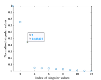
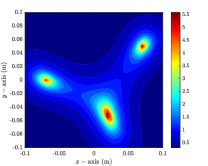
(a) with diagonal elements and $N=12$

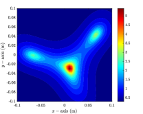
(b) without diagonal elements and $N=12$

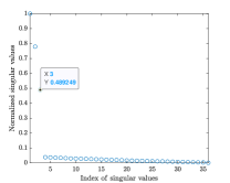
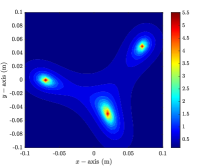
(c) with diagonal elements and $N=36$

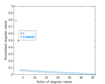
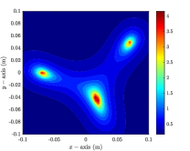
(d) without diagonal elements and $N=36$

Figure 2: (Example 5.1) Distribution of normalized singular values and maps of $\mathfrak{F}_{\operatorname*{TM}}(\mathbf{x})$ and $\mathfrak{F}_{\operatorname*{DM}}(\mathbf{x})$ at $f=$1\text{\,}\mathrm{GHz}$$.

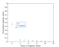
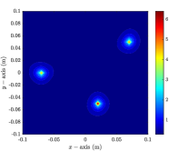
(a) with diagonal elements and $N=12$

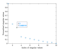
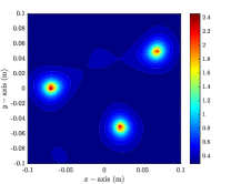
(b) without diagonal elements and $N=12$

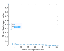
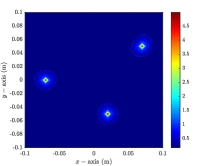
(c) with diagonal elements and $N=36$

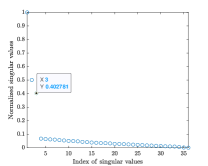
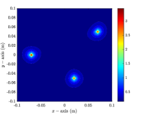
(d) without diagonal elements and $N=36$

Figure 3: (Example 5.1) Distribution of normalized singular values and maps of $\mathfrak{F}_{\operatorname*{TM}}(\mathbf{x})$ at $f=$2\text{\,}\mathrm{GHz}$$.

Example 5.2 (Magnetic permeability contrast case).

Figure 4 shows the maps of $\mathfrak{F}_{\operatorname*{TM}}(\mathbf{x})$ and $\mathfrak{F}_{\operatorname*{DM}}(\mathbf{x})$ with $f=$2\text{\,}\mathrm{GHz}$$ for $N=12$ and $N=36$ directions when $\varepsilon_{m}\equiv\varepsilon_{\mathrm{b}}$ and $\mu_{m}=5\mu_{\mathrm{b}}$. Opposite to the Example 5.1, it is impossible to recognize the existence of inhomogeneities with and without diagonal elements of the MSR matrix.

Based on the simulation result with $f=$4\text{\,}\mathrm{GHz}$$ with $N=12$ directions, it is still impossible to retrieve the inhomogeneities through the maps of $\mathfrak{F}_{\operatorname*{TM}}(\mathbf{x})$ and $\mathfrak{F}_{\operatorname*{DM}}(\mathbf{x})$. Moreover, it is very difficult to discriminate nonzero singular values of the MSR matrix without diagonal elements, refer to Figure 5. Fortunately, by increasing total number of directions $N=36$, it is very easy to discriminate nonzero singular values and possible to identify the existence of inhomogeneities by regarding the rings in the neighborhood of all $\mathbf{z}_{m}\in D_{m}$. This result supports the Remark 4.3 and we conclude that not only large number of directions $N$ but also high frequency $f$ must be applied to guarantee good imaging results.

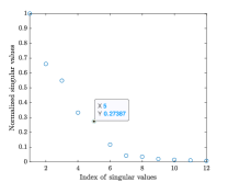
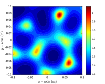
(a) with diagonal elements and $N=12$

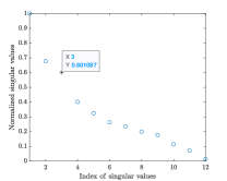
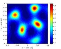
(b) without diagonal elements and $N=12$

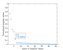
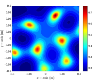
(c) with diagonal elements and $N=36$

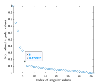
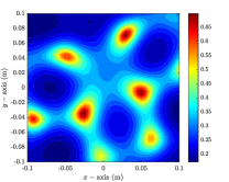
(d) without diagonal elements and $N=36$

Figure 4: (Example 5.2) Distribution of normalized singular values and maps of $\mathfrak{F}_{\operatorname*{TM}}(\mathbf{x})$ at $f=$2\text{\,}\mathrm{GHz}$$.

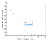
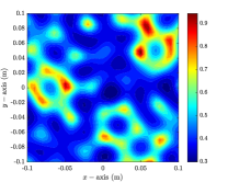
(a) with diagonal elements and $N=12$

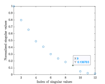
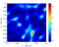
(b) without diagonal elements and $N=12$

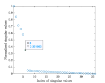
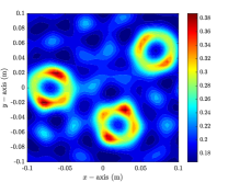
(c) with diagonal elements and $N=36$

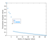
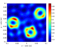
(d) without diagonal elements and $N=36$

Figure 5: (Example 5.2) Distribution of normalized singular values and maps of $\mathfrak{F}_{\operatorname*{TM}}(\mathbf{x})$ at $f=$4\text{\,}\mathrm{GHz}$$.

Example 5.3 (Simulation results with experimental data).

Here, we let us consider the simulation results with experimental data [63]. Following to the simulation configuration in the presence of two dielectric objects (twodielTM 8f.exp), the range of receivers is restricted from $60\text{\,}\mathrm{\SIUnitSymbolDegree}$ to $300\text{\,}\mathrm{\SIUnitSymbolDegree}$, with a step size of $5\text{\,}\mathrm{\SIUnitSymbolDegree}$ based on each direction of the transmitters. The transmitters are evenly distributed with step sizes of $10\text{\,}\mathrm{\SIUnitSymbolDegree}$ from $0\text{\,}\mathrm{\SIUnitSymbolDegree}$ to $350\text{\,}\mathrm{\SIUnitSymbolDegree}$. As a result, many elements (totally, $36\times 23$ measurement data) including the diagonal of the matrix $\mathbb{K}\in\mathbb{C}^{36\times 72}$ cannot be measured, We refer to Figure 6.

Although, the range of the $\mathbb{K}$ is unknown, we consider the application of the MUSIC. To this end, let us perform the SVD

$$\mathbb{K}=\sum_{n=1}^{N}\sigma_{n}\mathbf{U}_{n}\mathbf{V}_{n}^{*}\approx\sum_{n=1}^{N^{\prime}}\sigma_{n}\mathbf{U}_{n}\mathbf{V}_{n}^{*}.$$

Since $\mathbb{K}$ is non-symmetric, we cannot use the test vector $\mathbf{f}_{\varepsilon}(\mathbf{x})$ of (7) directly. Instead, based on the recent studies [22, 61], we generate projection operators onto the noise subspaces

$$\mathbb{P}_{\operatorname*{noise}}=\mathbb{I}_{N^{\prime}}-\sum_{n=1}^{N^{\prime}}\mathbf{U}_{n}\mathbf{U}_{n}^{*}\quad\text{and}\quad\mathbb{Q}_{\operatorname*{noise}}=\mathbb{I}_{N^{\prime}}-\sum_{n=1}^{N^{\prime}}\mathbf{V}_{n}\mathbf{V}_{n}^{*},$$

and unit test vectors

$$\mathbf{f}(\mathbf{x})=\frac{1}{\sqrt{36}}\bigg{(}e^{ik_{\mathrm{b}}\boldsymbol{\theta}_{1}\cdot\mathbf{x}},e^{ik_{\mathrm{b}}\boldsymbol{\theta}_{2}\cdot\mathbf{x}},\ldots,e^{ik_{\mathrm{b}}\boldsymbol{\theta}_{36}\cdot\mathbf{x}}\bigg{)}^{T}\quad\text{and}\quad\mathbf{g}(\mathbf{x})=\frac{1}{\sqrt{72}}\bigg{(}e^{-ik_{\mathrm{b}}\boldsymbol{\vartheta}_{1}\cdot\mathbf{x}},e^{-ik_{\mathrm{b}}\boldsymbol{\vartheta}_{2}\cdot\mathbf{x}},\ldots,e^{-ik_{\mathrm{b}}\boldsymbol{\vartheta}_{72}\cdot\mathbf{x}}\bigg{)}^{T}.$$

Then, the imaging function can be introduced as

$$\mathfrak{F}_{\operatorname*{DM}}(\mathbf{z})=\frac{1}{2}\left(\frac{1}{|\mathbb{P}_{\operatorname*{noise}}(\mathbf{f}(\mathbf{x}))|}+\frac{1}{|\mathbb{Q}_{\operatorname*{noise}}(\mathbf{g}(\mathbf{x}))|}\right).$$

Based on the imaging results in Figure 5.3, although exact shape of objects cannot be retrieved, the existence and outline shape of objects can be retrieved at $f=$4\text{\,}\mathrm{GHz}$$ and $6\text{\,}\mathrm{GHz}$. However, if one applies low frequency, it will be impossible to recognize the existence of objects (at $f=$1\text{\,}\mathrm{GHz}$$) or very difficult to retrieve the outline shape of objects (at $f=$2\text{\,}\mathrm{GHz}$$).

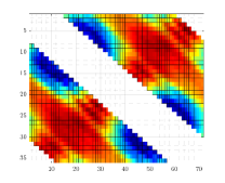
(a) $f=$1\text{\,}\mathrm{GHz}$$

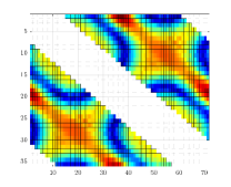
(b) $f=$2\text{\,}\mathrm{GHz}$$

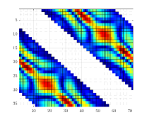
(c) $f=$4\text{\,}\mathrm{GHz}$$

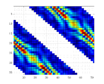
(d) $f=$6\text{\,}\mathrm{GHz}$$

Figure 6: (Example 5.3) Visualization of the absolute value of MSR matrix.

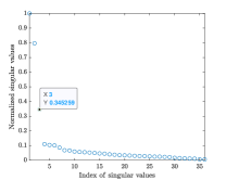
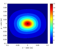
(a) $f=$1\text{\,}\mathrm{GHz}$$

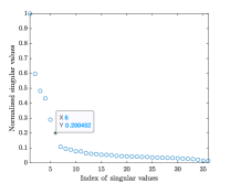
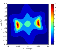
(b) $f=$2\text{\,}\mathrm{GHz}$$

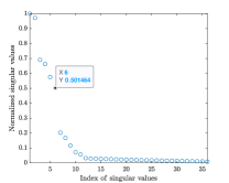
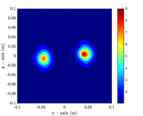
(c) $f=$4\text{\,}\mathrm{GHz}$$

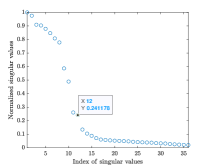
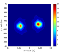
(d) $f=$6\text{\,}\mathrm{GHz}$$

Figure 7: (Example 5.3) Distribution of normalized singular values and maps of $\mathfrak{F}_{\operatorname*{DM}}(\mathbf{x})$.

6 Conclusion

In this study, we considered the MUSIC algorithm for localizing two-dimensional small inhomogeneity modeled via TM and TE polarization when the diagonal elements of MSR matrix cannot be determined. We investigated a mathematical structure of the imaging functions by establishing a relationship with the Bessel function of order $0$ (TM polarization) and $1$ (TE polarization). Based on the investigated structures, we confirmed that MUSIC can be applied to retrieve location of small inhomogeneity without the diagonal elements of the MSR matrix in both TM and TE polarizations.

Unfortunately, exact expression of $C_{\mu}$ in Theorem 4.6 is still unknown. Derivation of exact structure of the imaging function in TE polarization will be an interesting research subject. In this study, the structures were derived in the presence of single inhomogeneity but MUSIC can be applied to the identification of multiple, small inhomogeneities on the basis of simulation results. Extension to the multiple, small inhomogeneities will be the forthcoming work. Finally, extension to the three-dimensional inverse scattering problem will be an interesting research topic.

References

Ammari et al. [2005a]
H. Ammari, E. Iakovleva,
D. Lesselier, Two numerical methods for
recovering small electromagnetic inclusions from scattering amplitude at a
fixed frequency, SIAM J. Sci. Comput.
27 (2005a)
130–158.
Ammari et al. [2003a]
H. Ammari, E. Iakovleva,
S. Moskow, Recovery of small
inhomogeneities from the scattering amplitude at a fixed frequency,
SIAM J. Math. Anal. 34
(2003a) 882–900.
Ammari and Kang [2004]
H. Ammari, H. Kang,
Reconstruction of Small Inhomogeneities from Boundary
Measurements, vol. 1846 of Lecture
Notes in Mathematics, Springer-Verlag,
Berlin, 2004.
Ammari et al. [2003b]
H. Ammari, S. Moskow,
M. Vogelius, Boundary integral formulas for
the reconstruction of electromagnetic imperfections of small diameter,
ESAIM: Control Optim. Calc. Var. 9
(2003b) 49–66.
Bonnet [2008]
M. Bonnet, Inverse acoustic scattering by
small-obstacle expansion of a misfit function, Inverse
Probl. 24 (3) (2008)
Article No. 035022.
Dorn and Lesselier [2006]
O. Dorn, D. Lesselier,
Level set methods for inverse scattering,
Inverse Probl. 22 (2006)
R67–R131.
Smith and Hernandez [2019]
C. B. Smith, E. M. Hernandez,
Non-negative constrained inverse eigenvalue problems –
Application to damage identification, Mech. Syst. Signal
Proc. 129 (15) (2019)
629–644.
Zetik and Thoma [2008]
R. Zetik, R. S. Thoma,
Monostatic imaging of small objects in UWB sensor
networks, in: 2008 IEEE International Conference on
Ultra-Wideband, vol. 2, 191–194,
2008.
Kress [2003]
R. Kress, Newton’s method for inverse
obstacle scattering meets the method of least squares,
Inverse Probl. 19 (2003)
S91–S104.
Kristensen and Martinez-Panedab [2020]
P. K. Kristensen, E. Martinez-Panedab,
Phase field fracture modelling using quasi-Newton methods
and a new adaptive step scheme, Theor. Appl. Fract. Mec.
107 (2020) Article No.
102446.
Wick [2017]
T. Wick, Modified Newton methods for solving
fully monolithic phase-field quasi-static brittle fracture propagation,
Comput. Meth. Appl. Mech. Eng. 325
(2017) 577–611.
Álvarez et al. [2009]
D. Álvarez, O. Dorn,
N. Irishina, M. Moscoso,
Crack reconstruction using a level-set strategy,
J. Comput. Phys. 228
(2009) 5710–5721.
Park and Lesselier [2009a]
W.-K. Park, D. Lesselier,
Reconstruction of thin electromagnetic inclusions by a level
set method, Inverse Probl. 25
(2009a) Article No. 085010.
Ventura et al. [2002]
G. Ventura, J. X. Xu,
T. Belytschko, A vector level set method
and new discontinuity approximations for crack growth by EFG,
Int. J. Numer. Meth. Engng. 54
(2002) 923–944.
Kirsch and Grinberg [2008]
A. Kirsch, N. Grinberg, The
Factorization Method for Inverse Problems, Oxford
University Press, 2008.
Leem et al. [2020]
K. H. Leem, J. Liu,
G. Pelekanos, An extended direct
factorization method for inverse scattering with limited aperture data,
Inverse Probl. Sci. Eng.
28 (6) (2020)
754–776.
Park [2020]
W.-K. Park, Experimental validation of the
factorization method to microwave imaging, Results Phys.
17 (2020) Article No.
103071.
Ikeda et al. [1991]
K. Ikeda, M. Yoshimi,
C. Miki, Electrical potential drop method
for evaluating crack depth, Int. J. Fract.
47 (1991) 25–38.
Alves and Serranho [2004]
C. J. S. Alves, P. Serranho,
On the identification of the flatness of a sound-hard
acoustic crack, Math. Comput. Simulat.
66 (2004) 337–353.
Ammari et al. [2011]
H. Ammari, J. Garnier,
H. Kang, W.-K. Park,
K. Sølna, Imaging schemes for perfectly
conducting cracks, SIAM J. Appl. Math.
71 (1) (2011)
68–91.
Park [2019]
W.-K. Park, Real-time microwave imaging of
unknown anomalies via scattering matrix, Mech. Syst.
Signal Proc. 118 (2019)
658–674.
Park [2022a]
W.-K. Park, Real-time detection of small
anomaly from limited-aperture measurements in real-world microwave imaging,
Mech. Syst. Signal Proc. 171
(2022a) Article No. 108937.
Bonnet [2011]
M. Bonnet, Fast identification of cracks
using higher-order topological sensitivity for 2-D potential problems,
Eng. Anal. Bound. Elem. 35
(2011) 223–235.
Park [2013]
W.-K. Park, Multi-frequency topological
derivative for approximate shape acquisition of curve-like thin
electromagnetic inhomogeneities, J. Math. Anal. Appl.
404 (2013) 501–518.
Park [2012]
W.-K. Park, Topological derivative strategy
for one-step iteration imaging of arbitrary shaped thin, curve-like
electromagnetic inclusions, J. Comput. Phys.
231 (2012) 1426–1439.
Ito et al. [2012]
K. Ito, B. Jin, J. Zou,
A direct sampling method to an inverse medium scattering
problem, Inverse Probl.
28 (2) (2012)
Article No. 025003.
Kang et al. [2018]
S. Kang, M. Lambert, W.-K.
Park, Direct sampling method for imaging small dielectric
inhomogeneities: analysis and improvement, Inverse Probl.
34 (2018) Article No.
095005.
Kang et al. [2019]
S. Kang, M. Lambert, W.-K.
Park, Analysis and improvement of direct sampling method in
the mono-static configuration, IEEE Geosci. Remote Sens.
Lett. 16 (11) (2019)
1721–1725.
Cheney [2001]
M. Cheney, The linear sampling method and the
MUSIC algorithm, Inverse Probl. 17
(2001) 591–595.
Cakoni and Colton [2003]
F. Cakoni, D. Colton, The
linear sampling method for cracks, Inverse Probl.
19 (2003) 279–295.
Kirsch and Ritter [2000]
A. Kirsch, S. Ritter, A
linear sampling method for inverse scattering from an open arc,
Inverse Probl. 16 (1)
(2000) 89–105.
Ammari et al. [2007]
H. Ammari, E. Iakovleva,
D. Lesselier, G. Perrusson,
MUSIC type electromagnetic imaging of a collection of small
three-dimensional inclusions, SIAM J. Sci. Comput.
29 (2) (2007)
674–709.
Chen and Agarwal [2008]
X. Chen, K. Agarwal, MUSIC
algorithm for two-dimensional inverse problems with special characteristics
of cylinders, IEEE Trans. Antennas Propag.
56 (2008) 1080–1812.
Ammari et al. [2005b]
H. Ammari, E. Iakovleva,
D. Lesselier, A MUSIC algorithm for
locating small inclusions buried in a half-space from the scattering
amplitude at a fixed frequency, Multiscale Model. Sim.
3 (2005b)
597–628.
Iakovleva et al. [2007]
E. Iakovleva, S. Gdoura,
D. Lesselier, G. Perrusson,
Multi-static response matrix of a 3D inclusion in half
space and MUSIC imaging, IEEE Trans. Antennas Propag.
55 (2007) 2598–2609.
Griesmaier [2009]
R. Griesmaier, Reciprocity gap MUSIC
imaging for an inverse scattering problem in two-layered media,
Inverse Probl. Imag. 3
(2009) 389–403.
Song et al. [2012]
R. Song, R. Chen,
X. Chen, Imaging three-dimensional
anisotropic scatterers in multi-layered medium by MUSIC method with
enhanced resolution, J. Opt. Soc. Am. A
29 (2012) 1900–1905.
Ammari et al. [2008]
H. Ammari, H. Kang,
E. Kim, K. Louati,
M. Vogelius, A MUSIC-type algorithm for
detecting internal corrosion from electrostatic boundary measurements,
Numer. Math. 108 (2008)
501–528.
Bao et al. [2020]
Q. Bao, S. Yuan, F. Guo,
A new synthesis aperture-MUSIC algorithm for damage
diagnosis on complex aircraft structures, Mech. Syst.
Signal Proc. 136 (2020)
Article No. 106491.
Ammari et al. [2010]
H. Ammari, H. Kang,
H. Lee, W.-K. Park,
Asymptotic imaging of perfectly conducting cracks,
SIAM J. Sci. Comput. 32
(2010) 894–922.
Park [2015a]
W.-K. Park, Asymptotic properties of
MUSIC-type imaging in two-dimensional inverse scattering from thin
electromagnetic inclusions, SIAM J. Appl. Math.
75 (1)
(2015a) 209–228.
Park and Lesselier [2009b]
W.-K. Park, D. Lesselier,
Electromagnetic MUSIC-type imaging of perfectly conducting,
arc-like cracks at single frequency, J. Comput. Phys.
228 (2009b)
8093–8111.
Park and Lesselier [2009c]
W.-K. Park, D. Lesselier,
MUSIC-type imaging of a thin penetrable inclusion from its
far-field multi-static response matrix, Inverse Probl.
25 (2009c)
Article No. 075002.
Ammari et al. [2012]
H. Ammari, J. Garnier,
H. Kang, M. Lim,
K. Sølna, Multistatic imaging of
extended targets, SIAM J. Imag. Sci.
5 (2) (2012)
564–600.
Hou et al. [2006]
S. Hou, K. Sølna,
H. Zhao, A direct imaging algorithm for
extended targets, Inverse Probl. 22
(2006) 1151–1178.
Labyed and Huang [2012]
Y. Labyed, L. Huang,
Ultrasound time-reversal MUSIC imaging of extended
targets, Ultrasound Med. Biol.
38 (11) (2012)
2018–2030.
Marengo et al. [2007]
E. A. Marengo, F. K. Gruber,
F. Simonetti, Time-reversal MUSIC imaging
of extended targets, IEEE Trans. Image Process.
16 (8) (2007)
1967–1984.
Odendaal et al. [1994]
J. W. Odendaal, E. Barnard,
C. W. I. Pistorius, Two-dimensional
superresolution radar imaging using the MUSIC algorithm,
IEEE Trans. Antennas Propag. 42
(1994) 1386–1391.
Ruvio et al. [2013]
G. Ruvio, R. Solimene,
A. D’Alterio, M. J. Ammann,
R. Pierri, RF breast cancer detection
employing a noncharacterized vivaldi antenna and a MUSIC-inspired algorithm,
Int. J. RF Microwave Comput. Aid. Eng.
23 (5) (2013)
598–609.
Ruvio et al. [2014]
G. Ruvio, R. Solimene,
A. Cuccaro, D. Gaetano,
J. E. Browne, M. J. Ammann,
Breast cancer detection using interferometric MUSIC:
experimental and numerical assessment, Med. Phys.
41 (10) (2014)
Article No. 103101.
Scholz [2002]
B. Scholz, Towards virtual electrical breast
biopsy: space frequency MUSIC for trans-admittance data,
IEEE Trans. Med. Imag. 21
(2002) 588–595.
Chen and Zhong [2009]
X. Chen, Y. Zhong, MUSIC
electromagnetic imaging with enhanced resolution for small inclusions,
Inverse Probl. 25 (2009)
Article No. 015008.
Fannjiang [2011]
A. C. Fannjiang, The MUSIC algorithm for
sparse objects: a compressed sensing analysis, Inverse
Probl. 27 (3) (2011)
Article No. 035013.
Henriksson et al. [2011]
T. Henriksson, M. Lambert,
D. Lesselier, Non-iterative MUSIC-type
algorithm for eddy-current nondestructive evaluation of metal plates, in:
Electromagnetic Nondestructive Evaluation (XIV),
vol. 35 of Studies in Applied
Electromagnetics and Mechanics, 22–29,
2011.
Kirsch [2002]
A. Kirsch, The MUSIC algorithm and the
factorization method in inverse scattering theory for inhomogeneous media,
Inverse Probl. 18 (2002)
1025–1040.
Sekihara et al. [1999]
K. Sekihara, S. Nagarajan,
D. Poeppel, Y. Miyashita,
Time-frequency MEG-MUSIC algorithm, IEEE
Trans. Med. Imag. 18 (1)
(1999) 92–97.
Zhong and Chen [2007]
Y. Zhong, X. Chen, MUSIC
imaging and electromagnetic inverse scattering of multiple-scattering small
anisotropic spheres, IEEE Trans. Antennas Propag.
55 (2007) 3542–3549.
Ahn et al. [2015]
C. Y. Ahn, K. Jeon, W.-K.
Park, Analysis of MUSIC-type imaging functional for
single, thin electromagnetic inhomogeneity in limited-view inverse scattering
problem, J. Comput. Phys. 291
(2015) 198–217.
Joh et al. [2014]
Y.-D. Joh, Y. M. Kwon,
W.-K. Park, MUSIC-type imaging of
perfectly conducting cracks in limited-view inverse scattering problems,
Appl. Math. Comput. 240
(2014) 273–280.
Kang and Park [2022]
S. Kang, W.-K. Park,
Application of MUSIC algorithm for a fast identification of
small perfectly conducting cracks in limited-aperture inverse scattering
problem, Comput. Math. Appl. 117
(2022) 97–112.
Park [2022b]
W.-K. Park, A novel study on the MUSIC-type
imaging of small electromagnetic inhomogeneities in the limited-aperture
inverse scattering problem, J. Comput. Phys.
460 (2022b)
Article No. 111191.
Park [2023]
W.-K. Park, On the application of MUSIC
algorithm for identifying short sound-hard arcs in limited-view inverse
acoustic problem, Wave Motion 117
(2023) Article No. 103114.
Belkebir and Saillard [2001]
K. Belkebir, M. Saillard,
Special section: Testing inversion algorithms against
experimental data, Inverse Probl. 17
(2001) 1565–1571.
Park [2018]
W.-K. Park, Reconstruction of thin
electromagnetic inhomogeneity without diagonal elements of a multi-static
response matrix, Inverse Probl. 34
(2018) Article No. 095008.
Park [2021]
W.-K. Park, Application of MUSIC algorithm
in real-world microwave imaging of unknown anomalies from scattering matrix,
Mech. Syst. Signal Proc. 153
(2021) Article No. 107501.
Son et al. [2019]
S.-H. Son, K.-J. Lee,
W.-K. Park, Application and analysis of
direct sampling method in real-world microwave imaging,
Appl. Math. Lett. 96
(2019) 47–53.
Son et al. [2010]
S.-H. Son, N. Simonov,
H.-J. Kim, J.-M. Lee,
S.-I. Jeon, Preclinical prototype
development of a microwave tomography system for breast cancer detection,
ETRI J. 32 (2010)
901–910.
Cherniakov [2007]
M. Cherniakov, Bistatic Radar: Principles and
Practice, Wiley, 2007.
Comblet et al. [2006]
F. Comblet, A. Khenchaf,
A. Baussard, F. Pellen,
Bistatic synthetic aperture radar imaging: theory,
simulations, and validations, IEEE Trans. Antennas
Propag. 54 (11) (2006)
3529–3540.
Li et al. [2018]
T. Li, K.-S. Chen,
M. Jin, Analysis and simulation on imaging
performance of backward and forward bistatic synthetic aperture radar,
Remote Sensing 10 (11)
(2018) Article No. 1676.
Liang et al. [2019]
B. Liang, X. Shang,
X. Zhuge, J. Miao,
Bistatic cylindrical millimeter-wave imaging for accurate
reconstruction of high-contrast concave objects, Opt.
Express 27 (10) (2019)
14881–14892.
Qi et al. [2011]
Y. Qi, W. Tan, Y. Wang,
W. Hong, Y. Wu, 3D
bistatic Omega-K imaging algorithm for near range microwave imaging
systems with bistatic planar scanning geometry, Prog.
Electromagn. Res. 121 (2011)
409–431.
Rao and Chen [2006]
T. Rao, X. Chen, Analysis
of the time-reversal operator for a single cylinder under two-dimensional
settings, J. Electromagn. Waves Appl.
20 (15) (2006)
2153–2165.
Vogelius and Volkov [2000]
M. Vogelius, D. Volkov,
Asymptotic formulas for perturbations in the electromagnetic
fields due to the presence of inhomogeneities of small diameter,
ESAIM: M2AN 34 (4)
(2000) 723–748.
Park [2015b]
W.-K. Park, Multi-frequency subspace
migration for imaging of perfectly conducting, arc-like cracks in full- and
limited-view inverse scattering problems, J. Comput.
Phys. 283 (2015b)
52–80.
Park [2017]
W.-K. Park, A novel study on subspace
migration for imaging of a sound-hard arc, Comput. Math.
Appl. 74 (12) (2017)
3000–3007.
Huang et al. [2010]
K. Huang, K. Sølna,
H. Zhao, Generalized Foldy-Lax
formulation, J. Comput. Phys. 229
(2010) 4544–4553.