Dual-Space Optimization: Improved Molecule Sequence Design by
Latent Prompt Transformer

Abstract

Designing molecules with desirable properties, such as drug-likeliness and high binding affinities towards protein targets, is a challenging problem. In this paper, we propose the Dual-Space Optimization (DSO) method that integrates latent space sampling and data space selection to solve this problem. DSO iteratively updates a latent space generative model and a synthetic dataset in an optimization process that gradually shifts the generative model and the synthetic data towards regions of desired property values. Our generative model takes the form of a Latent Prompt Transformer (LPT) where the latent vector serves as the prompt of a causal transformer. Our extensive experiments demonstrate effectiveness of the proposed method, which sets new performance benchmarks across single-objective, multi-objective and constrained molecule design tasks.

1 Introduction

In drug discovery, identifying or designing molecules with specific pharmacological or chemical attributes, such as enhanced drug-likeness or high binding affinity to target proteins, is of paramount importance. However, navigating the vast space of potential drug-like molecules presents a daunting challenge.

To address this problem, several contemporary research avenues have emerged. One prominent approach involves the application of latent space generative models. This approach strives to translate the discrete molecule graph into a more manageable continuous latent vector. Once translated, molecular properties can be optimized within the continuous latent space utilizing various strategies (Gómez-Bombarelli et al., 2018; Kusner et al., 2017; Jin et al., 2018; Eckmann et al., 2022; Kong et al., 2023). Another avenue of research is more direct, employing combinatorial optimization methods such as reinforcement learning algorithms to fine-tune molecular attributes directly within the molecule graph data space (You et al., 2018; De Cao & Kipf, 2018; Zhou et al., 2019; Shi et al., 2020; Luo et al., 2021; Du et al., 2022). Diverse alternative methodologies in the data space have also gained traction, such as genetic algorithms (Nigam et al., 2020), particle-swarm strategies (Winter et al., 2019), Monte Carlo tree search (Yang et al., 2020), and scaffolding tree (Fu et al., 2021).

In this paper, we propose a Dual-Space Optimization (DSO) method that integrates latent space sampling and data space selection for molecule design. DSO iteratively updates a latent space generative model and a synthetic dataset in the optimization process that gradually shifts the generative model and the synthetic data towards regions of desired property values. The latent space generative model in DSO is realized by our proposed Latent Prompt Transformer (LPT) model that is comprised of three components: a prior model of the latent vector based on a neural transformation of Gaussian noise, a molecule generation model that generates molecule sequence by a causal transformer with the latent vector serving as the prompt, and a property predictor model that estimates the value of the target property given the latent vector.

Our method that leverages a confluence of latent and data spaces for optimization substantially outperforms baselines on several molecule design tasks. One task of particular interest is the conditional generation of molecules that bind to the NAD binding site of Phosphoglycerate dehydrogenase (PHGDH). We show that our model can both match and outperform human designed molecules given the same initial molecular backbone.

In summary, our contributions are as follows:

• Develop the Dual-Space Optimization (DSO) approach, integrating latent space sampling and data space selection in an iterative algorithm.

• Introduce a novel Latent Prompt Transformer model (LPT) for joint modeling of molecule sequences and their target properties, including pretraining and finetuning strategies.

• Demonstrate versatility of DSO with LPT, adaptable to a variety of tasks such as single-objective, multi-objective, and constrained optimization.

• Study the Phosphoglycerate dehydrogenase (PHGDH) with its NAD binding site, offering a benchmark for de novo design.

• Comprehensive experiments demonstrate the state-of-the-art performances of DSO across a wide range of molecule design tasks.

2 Problem Setup and Overview

Let $x=(x^{(1)},...,x^{(t)},...,x^{(T)})\in\mathcal{X}$ be a sequence representation of molecules (e.g. SMILES (Weininger, 1988) or SELFIES (Krenn et al., 2020; Cheng et al., 2023)), where $x^{(t)}\in\mathcal{V}$ is the $t$-th element in the vocabulary $\mathcal{V}$, and $\mathcal{X}$ is the space of molecules. In molecule design, the objective is to generate targeted molecules optimizing several properties of interest $\bm{y}=\{y_{i}=o^{p}_{i}(x)\in\mathbb{R}\}_{i=1}^{m}$ while adhering to specific constraints $\bm{c}=\{c_{j}=o^{c}_{j}(x)\in\mathbb{Z}_{2}\}_{j=1}^{n}$. Here $o^{p}(x)$ and $o^{c}(x)$ are oracle functions determining property values and constraint satisfaction, respectively. They are black-box functions whose output values can be obtained by querying existing software, such as RDKit (Landrum et al., ) and AutoDock-GPU (Santos-Martins et al., 2021). The multi-objective multi-constraint optimization (MMO) is defined as

$$\begin{split}\max_{x\in\mathcal{X}}\quad&F(x)=\{o^{p}_{1}(x),o^{p}_{2}(x),\dots,o^{p}_{m}(x)\}\\ \mathrm{s.t.}\quad&o^{c}_{j}(x)=1,\quad j=1,\ldots,n,\end{split}$$ (1)

where $o^{c}(x)=1$ denotes constraint satisfaction and $o^{c}(x)=0$ denotes constraint violation.

In the context of probabilistic modeling, the aforementioned problem is closely related to a conditional sampling problem,

$$x^{*}\sim p(x|\bm{y}=\bm{y}^{*},\bm{c}=\bm{1})$$ (2)

where $\bm{y}^{*}$ are desired values of the target properties and $\bm{c}=\bm{1}$ means all constraints are met. Note that both the property optimization and the constraint satisfaction problems are collectively addressed as multi-condition sampling problems. To simplify the notation, we shall use $y$ to represent both properties and constraints and $o(x)$ to represent the oracle functions for both properties and constraints in the following sections.

Molecule optimization in chemical (data) space typically involves iterative combinatorial search to generate proposals (e.g., $x\sim p(x|y^{*})$), coupled with oracle functions for obtaining ground-truth property values (e.g., $y=o(x)$). The discrete nature and the immense size of the search space greatly complicates the problem.

To address this challenge, we propose a Dual-Space Optimization (DSO) framework that integrates latent space sampling and data space selection for molecule design. DSO iteratively updates a latent space generative model and a synthetic dataset in the optimization process that gradually shifts the generative model and the synthetic data towards regions of desired property values.

We propose a novel latent space generative model, Latent Prompt Transformer (LPT), which jointly models the molecule sequences and properties as $p(x,y)=\int p(z,x,y)dz$. Conditional on the low-dimensional latent vector $z\in\mathbb{R}^{d}$, we assume the molecule sequence $x$ and the value of the target property $y$ are independent so that the joint probability distribution $p(z,x,y)$ can be factorized into $p(z)p(x|z)p(y|z)$. $p(z)$, the prior distribution, is modeled by a neural transformation of an isotropic Gaussian distribution, i.e. $z=U_{\alpha}(z_{0})$, $z_{0}\sim\mathcal{N}(0,I_{d})$, where $U_{\alpha}$ is a neural network with parameters $\alpha$. $p(x|z)$ is a molecule sequence generation model, which can be modeled by a causal Transformer with the latent vector $z$ serving as the prompt, guiding each step of the generation process. $p(y|z)$ can either be a regression or classification model, designed to predict a property or determine constraint satisfaction. For simplicity, we refer $p(y|z)$ as the predictor model. Hence the sampling in the chemical space can be relaxed by performing it in the low-dimensional latent space. Given desired value $y^{*}$,

$$z^{*}\sim p(z|y=y^{*}),\quad{x}\sim p(x|z=z^{*}).$$ (3)

Note that the sampling in the latent space is guided by both prior and predictor models: $z^{*}\sim p(z|y^{*})\propto p(z)p(y^{*}|z)$ via the Bayes rule. To extend the capabilities of a well-trained model beyond its observed data range, we propose to iteratively adjust the desired value as $y^{*}=y+\Delta_{y}$, where $y$ is a high value that the model has previously encountered, and $\Delta_{y}$ is a small increment. This latent space sampling enables incremental extrapolation to generate new molecules. We then use the oracle function in the data space to select the set of samples $(x^{*},y^{*})$ with optimal property values, which are used to improve the LPT thereafter. This procedure of latent space sampling, data space selection, and LPT improvement is repeated in multiple rounds, allowing for gradually shifting the latent space generative model and a set of samples towards regions of desired properties.

3 Latent Prompt Transformer (LPT)

3.1 Model

Suppose $x=(x^{(1)},...,x^{(t)},...,x^{(T)})$ is a molecule sequence, (e.g. a string-based molecule as in SELFIES (Krenn et al., 2020)), $z\in\mathbb{R}^{d}$ is the latent vector. $y\in\mathbb{R}$ is the value of the target property of interest, or $y\in\{0,1\}$ is the indication of constraint satisfaction.

Figure 1: Left: Overview of Latent Prompt Transformer (LPT). Right: Detailed illustration of generation model $p_{\beta}(x|z)$.

As shown in Fig. 1, we define the following latent variable model as the latent prompt Transformer (LPT):

$$z\sim p_{\alpha}(z),\quad[x|z]\sim p_{\beta}(x|z),\quad[y|z]\sim p_{\gamma}(y|z),$$ (4)

where $p_{\alpha}(z)$ is a prior model with parameters $\alpha$. $z$ serves as the latent prompt of the generation model $p_{\beta}(x|z)$ parameterized by a causal Transformer with parameter $\beta$. $p_{\gamma}(y|z)$ is the predictor model with parameter $\gamma$.

For the prior model, $p_{\alpha}(z)$ is formulated as a learnable neural transformation from an uninformative prior,

$$z=U_{\alpha}(z_{0}),$$ (5)

where $z_{0}$ is assumed to be isotropic Gaussian $\mathcal{N}(0,I_{d})$, and $U_{\alpha}(\cdot)$ is parametrized by an expressive neural network such as a Unet (Ronneberger et al., 2015) with parameter $\alpha$.

The generation model $p_{\beta}(x|z)$ is a conditional autoregressive model,

$$p_{\beta}(x|z)=\prod_{t=1}^{T}p_{\beta}(x^{(t)}|x^{(0)},...,x^{(t-1)},z)$$ (6)

which is parameterized by a causal Transformer with parameter $\beta$. Note that the latent vector $z$ controls every step of the autoregressive generation and it functions as a soft prompt that controls the generation of molecules. We incorporate latent vectors into our Transformer model through cross-attention. Details on model architectures are available in the Appendix A.

Given a molecule $x$, let $y$ denote the value of the target property, such as protein binding affinity or indication of drug-likeliness in a certain range. One can determine the estimated value of this property using open-source software such as RDKit (Landrum et al., ) and AutoDock-GPU (Santos-Martins et al., 2021).

Given $z$, we posit that $x$ and $y$ are conditionally independent and $z$ is the information bottleneck. Under this assumption, LPT defines the joint distribution,

$$p_{\theta}(x,y,z) =p_{\alpha}(z)p_{\beta}(x|z)p_{\gamma}(y|z),$$ (7)

where $\theta=(\alpha,\beta,\gamma)$. We use the marginal distribution $p_{\theta}(x,y)=\int p_{\theta}(x,y,z)dz$ to approximate the data distribution $p_{\mathrm{data}}(x,y)$.

For the property predictor, it can either be a regression model,

$$p_{\gamma}(y|z)=\frac{1}{\sqrt{2\pi\sigma^{2}}}\exp\left(-\frac{1}{2\sigma^{2}}(y-s_{\gamma}(z))^{2}\right),$$ (8)

or a constraint classifier,

$$p_{\gamma}(y|z)=s_{\gamma}(z)^{y}(1-s_{\gamma}(z))^{1-y}$$ (9)

where $s_{\gamma}(z)$ is a small multi-layer perceptron (MLP), predicting $y$ based on the latent prompt $z$. The variance $\sigma^{2}$ is treated as a hyper-parameter.

For tasks involving multi-objective design with target properties or multiple constraints $\bm{y}=\{y_{j}\}_{j=1}^{M}$, the above predictor can be extended to $p_{\gamma}(\bm{y}|z)=\prod_{j=1}^{M}p_{\gamma_{j}}(y_{i}|z)$, where each $p_{\gamma_{j}}(y_{i}|z)$ is parametrized as in Eq. 8 or Eq. 9.

Given this formulation, the learned latent prompt $z$ is aware of the properties and constraints while generating the molecule.

3.2 Learning

Suppose we observe training examples from the offline (collected) dataset $\mathcal{D}=\{(x_{i},y_{i}),i=1,...,n\}$. The log-likelihood function is $L(\theta)=\sum_{i=1}^{n}\log p_{\theta}(x_{i},y_{i})$.

Since $z=U_{\alpha}(z_{0})$, we can also write the model as

$$p_{\theta}(x,y)=\int p_{\beta}(x|z=U_{\alpha}(z_{0}))p_{\gamma}(y|z=U_{\alpha}(z_{0}))p_{0}(z_{0})dz_{0},$$ (10)

where $p_{0}(z_{0})\sim{\cal N}(0,I_{d})$. The learning gradient can be calculated according to

$$\begin{split}\nabla_{\theta}\log p_{\theta}(x,y)&=\mathbb{E}_{p_{\theta}(z_{0}|x,y)}[\nabla_{\theta}\log p_{\beta}(x|U_{\alpha}(z_{0}))\\ &+\nabla_{\theta}\log p_{\gamma}(y|U_{\alpha}(z_{0}))].\end{split}$$ (11)

For the prior model, the learning gradient is

$$\begin{split}\delta_{\alpha}(x,y)&=\mathbb{E}_{p_{\theta}(z_{0}|x,y)}[\nabla_{\alpha}\log p_{\beta}(x|U_{\alpha}(z_{0}))\\ &+\nabla_{\alpha}\log p_{\gamma}(y|U_{\alpha}(z_{0})))].\end{split}$$ (12)

The learning gradient for the generation model is

$$\begin{split}\delta_{\beta}(x,y)=\mathbb{E}_{p_{\theta}(z_{0}|x,y)}[\nabla_{\beta}\log p_{\beta}(x|U_{\alpha}(z_{0}))].\end{split}$$ (13)

The learning gradient for the predictor model is

$$\begin{split}\delta_{\gamma}(x,y)=\mathbb{E}_{p_{\theta}(z_{0}|x,y)}[\nabla_{\gamma}\log p_{\gamma}(y|U_{\alpha}(z_{0}))].\end{split}$$ (14)

Estimating expectations in Eqs. 12, 13 and 14 requires MCMC sampling of the posterior distribution $p_{\theta}(z_{0}|x,y)$. We recruit Langevin dynamics (Neal, 2011). For a target distribution $\pi(z)$, the dynamics iterates

$$z^{\tau+1}=z^{\tau}+s\nabla_{z}\log\pi(z^{\tau})+\sqrt{2s}\epsilon^{\tau},$$ (15)

where $\tau$ indexes the time step of the Langevin dynamics, $s$ is step size, and $\epsilon_{\tau}\sim{\mathcal{N}}(0,I_{d})$ is the Gaussian white noise. $\pi(z)$ here is the posterior $p_{\theta}(z_{0}|x,y)$, and the gradient can be efficiently computed by back-propagation. We initialize $z_{0}^{\tau=0}\sim{\mathcal{N}}(0,I_{d})$, and employ $N$ steps of Langevin dynamics (e.g. $N=15$) for approximate sampling from the posterior distribution, rendering our learning algorithm as an approximate maximum likelihood estimation. See (Pang et al., 2020; Nijkamp et al., 2020; Xie et al., 2023) for a theoretical understanding of the learning algorithm based on the finite-step MCMC.

Algorithm 1 Learning Latent Prompt Transformer (LPT)

  Input: Learning iterations $T$, initial parameters $\theta_{0}=(\alpha_{0},\beta_{0},\gamma_{0})$, observed samples $\mathcal{D}=\{x_{i},y_{i}\}_{i=1}^{n}$, posterior sampling step size $s$, the number of steps $N$, and the learning rate $\eta_{0},\eta_{1},\eta_{2}$.

  Output: $\theta_{T}$

  for $t=1$ to $T$ do

     1.Posterior sampling: For each $(x_{i},y_{i})$, sample $z_{0}\sim{p}_{\theta_{t}}(z_{0}|x_{i},y_{i})$ using Eq. 15, where the target distribution $\pi$ is ${p}_{\theta_{t}}(z_{0}|x_{i},y_{i})$.

     2.Learn prior model $p_{\alpha}(z)$, generation model $p_{\beta}(x|z)$ and predictor model $p_{\gamma}(y|z)$: Update $\theta_{t+1}$ via gradient ascent with Eqs. 12, 13 and 14

  end for

3.3 Pretrain and Finetune LPT

In practical applications with multiple molecular generation tasks, with each characterized by a different target property $y$, each model $p_{\theta}(x,y)$ may necessitate separate training. For the sake of efficiency, we adopt a two-stage training approach. In the first stage, we pretrain the model on molecules alone while ignoring the properties by maximizing $\sum_{i=1}^{n}\log p_{\theta}(x_{i})=\sum_{i=1}^{n}\log\int p_{\theta}(x_{i},z_{i})dz_{i}$. The learning gradient is

$$\nabla_{\theta}\log p_{\theta}(x)=\mathbb{E}_{p_{\theta}(z_{0}|x)}\left[\nabla_{\beta}\log p_{\theta}(x|U_{\alpha}(z_{0}))\right],$$ (16)

and the learning gradients for $\alpha$ and $\beta$ become

$$\delta_{\alpha}(x)=\mathbb{E}_{p_{\theta}(z_{0}|x)}[\nabla_{\alpha}\log p_{\beta}(x|U_{\alpha}(z_{0}))],$$ (17)

$$\delta_{\beta}(x)=\mathbb{E}_{p_{\theta}(z_{0}|x)}[\nabla_{\beta}\log p_{\beta}(x|U_{\alpha}(z_{0}))].$$ (18)

For estimating expectations in Eqs. 17 and 18, we use finite-step MCMC as in Eq. 15 by replacing the target distribution $\pi(z)$ by $p_{\theta}(z_{0}|x)$. In the second stage, we finetune the model with target properties using Eqs. 12, 13 and 14, as detailed in Alg. 1. This two-stage approach is adaptable for semi-supervised scenarios where property values are limited.

4 Dual-Space Optimization

Figure 2: Graphical illustration of Dual-Space Optimization (DSO) with LPT at the shifting iteration $t$. The plot of distribution shifting over iterations can be found in Fig. 3

.

After learning the joint distributions of molecules and properties $p_{\theta}(x,y)$, our objective is to generate a synthetic dataset of molecules with maximal values of specific target properties, as defined by oracle functions $o(x)$. Following previous studies on molecule design, we assume access to the oracle functions via software such as RDKit (Landrum et al., ) and AutoDock-GPU (Santos-Martins et al., 2021). While acknowledging the critical role of these tools in providing accurate property evaluations for molecules, our paper focuses primarily on the optimization process, not the designing of the oracle function.

In optimization cases where the target value $y^{*}$ may not be supported within the learned distribution $p_{\theta}(x,y)$, we introduce an iterative online optimization method. This process is initialized with a pretrained distribution $p_{\theta}(x,y)$ and gradually shifts the distribution over $T$ iterations.

Each iteration involves a dual-space sampling strategy: Latent Space Sampling for generating proposals and Data Space Selection for refinement of the synthetic dataset by the oracle function and Improve LPT based on the refined dataset, termed as Dual-Space Optimization (DSO). We provide an overview and a demonstration of the DSO in Fig. 2 and Fig. 3.

In this iterative framework, the optimization problem at iteration $t$ is as follows: Given the trained model at the previous time step $p_{\theta_{t-1}}(z,x,y)$ and the shifting dataset $\mathcal{D}^{t-1}=\{z_{i}^{t-1},x_{i}^{t-1},y_{i}^{t-1}\}_{i=1}^{n}$, we aim to sample proposals $\mathcal{P}^{t}=\{z_{i}^{t},x_{i}^{t},y_{i}^{t}\}$ to create an improved synthetic dataset $\mathcal{D}^{t}$. This new dataset is designed to exhibit improved desired properties over $\mathcal{D}^{t-1}$, allowing fitting and refining our model progressively. The initial dataset $\mathcal{D}^{0}$ is composed of the top-$n$ samples with desired values from the offline dataset $\mathcal{D}$.

Latent Space Sampling.

The latent space generative model enables incremental extrapolation for search, and we first sample proposals at the distribution boundary to ensure a reliable shifting. Specifically, we define

$$y^{t}=y^{t-1}+\Delta_{y}$$ (19)

where $y^{t-1}$ lies in the upper range of $\mathcal{D}^{t-1}$(e.g. the top $100$ values) and $\Delta_{y}$ is a fixed small increment to promote exploration beyond the current distribution.

The proposal $\mathcal{P}^{t}$ can be generated by ancestral sampling,

$$z_{0}\sim p_{\theta}(z_{0}|y)\propto p_{0}(z_{0})p_{\gamma}(y|z=U_{\alpha}(z_{0})),$$ (20)

and then let $z=U_{\alpha}(z_{0})$,

$$x\sim p(x|z=U_{\alpha}(z_{0})),$$ (21)

where we set $y=y^{t}$ and $\theta=\theta^{t-1}$. The Sampling in Eq. 20 can be realized by persistent Markov Chain (PMC) by iterating Eq. 15,

$$z_{0}^{\tau+1}=z_{0}^{\tau}+s\nabla_{z_{0}}(\log p_{0}(z_{0})+\log p_{\gamma}(y|U_{\alpha}(z_{0}))+\sqrt{2s}\epsilon^{\tau}.$$ (22)

Here, $z_{0}^{\tau=0}$ is initialized from the previous training step. With PMC, it is feasible to set the number of Langevin sampling steps to be relatively small, e.g. $N=2$. Consequently, the sampled $z$ is aware of the specific property values or constraints and regulated by the prior model.

Algorithm 2 Dual-Space Optimization (DSO)

  Input: Number of proposals $m$, fixed increment $\Delta_{y}$, number of PMC steps $N$, initial parameters $\theta_{t}=(\alpha_{t},\beta_{t},\gamma_{t})$, initial dataset $\mathcal{D}^{0}=\{z_{i}^{0},x_{i}^{0},y_{i}^{0}\}_{i=1}^{n}$, oracle function $o(x)$, maximum shifting iteration $T$.

  Output: $\theta^{T}$, $\mathcal{D}^{T}$

  while $\mathbb{E}_{p_{\theta}(x,y)}[o(x)]$ is increasing do

     1.Latent space sampling: Sample proposal $\mathcal{P}^{t}=\{z^{t}_{i},x^{t}_{i},y^{t}_{i}\}_{i=1}^{m}$, where $z^{t}\sim p(z|y=y^{t-1}+\Delta_{y})$ as in Eq. 20; $x^{t}\sim p(x|z=z^{t})$ as in  Eq. 21.

     2.Data space selection: Relabel proposal property values $y_{i}^{t}\to\check{y}_{i}^{t}=o(x_{i}^{t})$. Update dataset $\mathcal{D}^{t}=\mathrm{Select}(\{z_{i}^{t},x_{i}^{t},\check{y}_{i}^{t}\}_{i=1}^{m}\cup\mathcal{D}^{t-1})$ as in Eq. 23

     3.Improve LPT: Learn $\theta$ using Alg. 1 with $\mathcal{D}^{t}$.

  end while

Data Space Selection.

After generating the proposals $\mathcal{P}^{t}$, we use the oracle function $o(x)$ to relabel these proposals, $\check{y}=o(x)$, yielding a set of generated samples and their ground-truth property values as $\{z_{i}^{t},x_{i}^{t},\check{y}_{i}^{t}\}_{i=1}^{m}$.

The next step involves a select operation, designed to merge these proposals with the existing dataset to improve overall properties in the new dataset. For tasks focused on optimizing properties (i.e., maximizing specific values), this is achieved by ranking all samples and retaining the top-n entries, with n equaling the size of dataset $\mathcal{D}^{t-1}$. Alternatively, we can also choose samples that explicitly meet certain constraints.

The selection operation is defined as follows:

$$\mathcal{D}^{t}=\mathrm{Select}(\{z_{i}^{t},x_{i}^{t},\check{y}_{i}^{t}\}_{i=1}^{m}\cup\mathcal{D}^{t-1}).$$ (23)

This approach in the data space is a counterpart to our latent space sampling strategy. For instance, if the goal is to maximize a property $y_{1}$ while adhering to the constraint $y_{2}>c$, we would sample $z\sim p(z|y_{1},y_{2})\propto p(z)p(y_{1}|z)p(y_{2}|z)$ and rank the samples based on $\check{y}_{1}\mathds{1}(\check{y}_{2}>c)$, where c is a constant and $\mathds{1}(\cdot)$ is an indicator function.

Improve LPT.

With each generated synthetic dataset $\mathcal{D}^{t}$, we can improve the LPT using Alg. 1. The learning objective is,

$$\theta_{t}=\operatorname*{arg\,max}_{\theta}\mathbb{E}_{(x,y)\sim\mathcal{D}^{t}}[\log p_{\theta}(x,y)],$$ (24)

where $\theta$ is initialized from $\theta^{t-1}$. At the $t$-th shifting iteration, particularly in a single property maximization scenario, the top-$n$ selection as per Eq. 23 sets a threshold at $n$-th sample, denoted as $c^{t}$. This is because we only consider samples where $\check{y}^{t}=o(x^{t})>c^{t}$. Latent space sampling and data space selection collectively result in a new dataset as a mixture of original and the synthetic data distribution. Intuitively, training on synthetic data is a form of online learning, i.e. the samples are generated from the current model, while training on the original dataset is a form of offline learning that prevents the $\theta^{t}$ moving too far from the $\mathcal{D}^{t-1}$ to avoid mode collapse.

Compared to population-based methods such as genetic algorithms (Nigam et al., 2020) and particle-swarm algorithms (Winter et al., 2019), our method not only maintains a shifting dataset $\mathcal{D}^{t}$ (which can be considered a small population), but also a shifting model $\theta^{t}$ to fit the dataset, so that we can improve generated molecules from the model. The model itself is virtually an infinite population because it can generate infinitely many new samples.

Note that the select operation in Eq. 23 creates a series of non-decreasing thresholds, meaning $c^{t}\geq c^{t-1}$. DSO terminates when there is no further increase in $c_{t}$, indicating that $\mathbb{E}_{p_{\theta}(x,y)}[o(x)]$ is no longer increasing.

5 Experiments

We demonstrate the effectiveness of our approach across a wide range of optimization tasks. In molecule design, this includes single-objective Penalized logP (P-logP) and QED maximization (Sec. 5.2), binding affinity maximization, constrained optimization, and multi-objective optimization (Sec. 5.3). Additionally, we optimize protein sequences for high fluorescence and DNA sequences for enhanced binding affinity (Sec. 5.4). A detailed discussion of related works and baselines is provided in Appendix B.

Figure 3: Illustration of DSO of ACAA1 binding affinity across shifting iterations. For each shift iteration, we plot the densities of docking scores $E$ using AutoDock-GPU. The increase of the docking scores indicates better binding affinity.

5.1 Experiment Setup

5.1.1 Molecule Sequence Design

For molecule design tasks, we use ZINC (Irwin et al., 2012) with $250$k drug-like molecules as our offline dataset $\mathcal{D}$. We utilize RDKit (Landrum et al., ) to compute several key metrics: penalized logP, drug-likeness (QED), and the synthetic accessibility score (SA). Additionally, we use AutoDock-GPU (Santos-Martins et al., 2021) to derive docking scores $E$, which serve as proxies for estimating the binding affinity of compounds to three protein targets. These targets include the human estrogen receptor (ESR1), human peroxisomal acetyl-CoA acyl transferase 1 (ACAA1), and Phosphoglycerate dehydrogenase (PHGDH). The binding affinity is expressed in terms of the dissociation constant $K_{D}(\mathrm{nM})$.

ESR1 is a well-characterized protein with many known binders, making it a suitable reference point for evaluating molecules generated by our model, while ACAA1 has no known binders, providing an opportunity to test the model’s capability for de novo design (Eckmann et al., 2022).

Additionally, we propose to design molecules that bind to PHGDH, an enzyme pivotal in the early stages of L-serine synthesis. Recently, PHGDH has gained attention as a potential therapeutic target in cancer therapy, owing to its role in various human cancers (Zhao et al., 2020). The crystal structure of PHGDH (PDB: 2G76) is well-established, and there is a well-documented case study on the development of PHGDH inhibitors, showcasing a structure-based progression from simpler to more complex molecules targeting its NAD binding site (Spillier & Frédérick, 2021), as illustrated in Fig. 4. Furthermore, we observe that the $K_{D}$ values estimated from wet lab experiments align with the trends predicted by AutoDock-GPU. This congruence makes PHGDH-NAD an excellent case study for testing DSO on single-objective, structure-constrained, and multi-objective optimization tasks using AutoDock-GPU. More details can be found in  Appendix C.

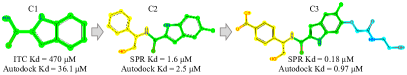
Figure 4: Development of PHGDH inhibitors (Spillier & Frédérick, 2021). Isothermal Titration Calorimetry (ITC), Surface Plasmon Resonance (SPR), and AutoDock $K_{D}$ values are measured for each inhibitor, showing that the trends between ITC/SPR and AutoDock values align well.

5.1.2 Protein and DNA Sequence Design

We further apply our method to biological sequence design to two tasks in Design-Bench (Trabucco et al., 2022): TF Bind 8 and GFP. The TF Bind 8 task aims to identify DNA sequences, each 8 bases long, with maximum binding affinity. This task contains a training set of 32,898 samples and includes an exact oracle function. The GFP task involves generating protein sequences of 237 amino acids that exhibit high fluorescence, and we use a subset of 5,000 samples as the training set following (Trabucco et al., 2022). Since an exact oracle function is unavailable for the GFP task, we follow the same oracle function preparation as in Design-Bench and train a Transformer regression model on the full dataset with 56,086 total samples as the oracle function. We evaluate the design performance and diversity of our generated samples.

5.1.3 Model Training Setup

The prior model, $p_{\alpha}(z)$, of LPT is parameterized by a 1-dimensional UNet (Ronneberger et al., 2015) where $z$ contains $4$ tokens each of size $256$. The sequence generation model, $p_{\beta}(x|z)$, is implemented as a 3-layer causal Transformer, and a 3-layer MLP acts as the predictor model, $p_{\gamma}(y|z)$. As described in Section 3.3, we pre-train LPT on molecules for 30 epochs then fine-tune with target properties for 10 epochs using Alg. 1. We perform up to 25 iterations of DSO, generating 2,500 samples per iteration, totaling a maximum of $62.5$k oracle queries. We use the AdamW optimizer (Loshchilov & Hutter, 2019; Kingma & Ba, 2014) with 0.1 weight decay. Training was conducted on an NVIDIA A6000 and took 20, 10, and 12 hours for pre-training LPT, fine-tuning LPT, and DSO respectively. More training details can be found at Appendix A.

5.2 Penalized logP and QED Maximization

Our first set of experiments focuses on optimizing the Penalized logP(P-logP) and QED properties, both of which can be calculated by RDKit. Since P-logP scores are positively correlated with the length of a molecule, we maximize Penalized logP while limiting molecule length to the maximum length of molecules in ZINC using the SELFIES (Krenn et al., 2020; Cheng et al., 2023) representation, following (Eckmann et al., 2022). From Table 1, we can see that DSO outperforms previous methods and achieves the highest QED for methods where molecule length is limited.

Table 1: P-logP and QED maximization. We report the top-3 highest scores achieved by each model. LL (Length Limit) indicates the application of a maximum molecule length limit. Baseline results are obtained from (Eckmann et al., 2022; You et al., 2018; Luo et al., 2021; Xie et al., 2021; Kong et al., 2023).

Method	LL	Penalized logP $(\uparrow)$			QED $(\uparrow)$
		1st	2rd	3rd	1st	2rd	3rd
JT-VAE	✗	5.30	4.93	4.49	0.925	0.911	0.910
GCPN	✓	7.98	7.85	7.80	0.948	0.947	0.946
MolDQN	✓	11.8	11.8	11.8	0.948	0.943	0.943
MARS	✗	45.0	44.3	43.8	0.948	0.948	0.948
GraphDF	✗	13.7	13.2	13.2	0.948	0.948	0.948
LIMO	✓	10.5	9.69	9.60	0.947	0.946	0.945
SGDS	✓	26.4	25.8	25.5	0.948	0.948	0.948
DSO	✓	38.95	38.29	38.25	0.948	0.948	0.948

5.3 Binding Affinity Maximization

5.3.1 Single-Objective Optimization

For the single-objective binding affinity optimization task, we aim to design ligands with optimal binding affinities to ESR1, ACAA1, and PHGDH as de novo design, without any constraints. DSO does not use any prior knowledge of existing binders, and exclusively uses the crystal structures of the aforementioned proteins. The predictor model $p_{\gamma}(y|z)$ for this task is a regression model that estimates docking scores. As shown in Tables 2 and 3, our model significantly surpasses other methods in all three binding affinity maximization tasks (measured by minimizing $K_{D}$), often by an order of magnitude. Furthermore, in Table 3, we present molecules with the top$-$100 scores to illustrate that our model can effectively generate a diverse pool of candidate molecules with the desired properties. Notably, our LPT-based DSO outperforms the Latent space Energy-based Model (LEBM)-based SGDS (Kong et al., 2023) in consistently sampling high-affinity molecules; we discuss further advantages in Appendix B.

Table 2: Single-objective binding affinity optimization. We report the top-3 $K_{D}\mathrm{(nM)}$ scores for each model (Eckmann et al., 2022; Kong et al., 2023).

Method	ESR1 $\mathrm{K_{D}}$ $(\downarrow)$			ACAA1 $\mathrm{K_{D}}$ $(\downarrow)$
	1st	2rd	3rd	1st	2rd	3rd
GCPN	6.4	6.6	8.5	75	83	84
MolDQN	373	588	1062	240	337	608
MARS	25	47	51	370	520	590
GraphDF	17	64	69	163	203	236
LIMO	0.72	0.89	1.4	37	37	41
SGDS	0.03	0.03	0.04	0.11	0.11	0.12
DSO	0.004	0.005	0.009	0.037	0.041	0.045

Table 3: PHGDH binding affinity maximization. We report the top-100 lowest $K_{D}(10^{-2}\mathrm{nM})$ for each model. Baselines are produced using official code.

Method	PHGDH $\mathrm{K_{D}}$ $(\downarrow)$
	1st	2rd	3rd	Top-50	Top-100
LIMO	13.87	18.79	21.15	81.16 $\pm$ 34.41	125.06 $\pm$ 52.59
SGDS	3.65	6.59	7.16	14.7 $\pm$ 5.43	24.5 $\pm$ 14.0
DSO	0.07	0.16	0.19	0.95 $\bf\pm 0.46$	1.66 $\bf\pm 0.82$

5.3.2 Structure-constrained Optimization

The structure-constrained optimization task is a conditional generation task that mirrors lead optimization in drug discovery, aiming to decorate a fixed core substructure to optimize activity and pharmacological properties.

Our model’s factorization, $p(z,x,y)=p(z)p(x|z)p(y|z)$, enables the decoupling of molecule generation and property prediction, facilitating its application in conditional generation. Given a substructure $\hat{x}=(x^{(1)},\dots,x^{(k)})$, we aim to sample from $p_{\theta}(x,y|\hat{x})$. This is accomplished by sampling $z\sim p(z|y)$ and then $x\sim p(x|\hat{x},z)$, simply requiring a rearrangement of $\hat{x}$’s sequence to start from the desired atom. In Fig. 4, Compound 2 (C2) is designed by humans as an extension of Compound 1 (C1), and Compound 3 (C3) is similarly an extension of C2. We show that: 1) given C1 or C2, our model can design similar compounds to human designed C2 or C3, and 2) our model can identify superior molecules compared to those designed by humans.

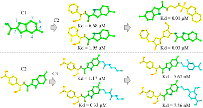
Figure 5: Structure-constrained Optimization. Conditionally generated C2 and C3 are almost identical to the human designed C2 and C3 in Fig. 4. Additionally, the right column shows further optimized compounds that achieve stronger $K_{D}$ scores.

Compound Analysis

Studies have documented numerous indole-based inhibitors for PHGDH (Spillier & Frédérick, 2021). In this experiment, we use our model to explore high-affinity inhibitors by adding functional groups to the second and sixth positions of an indole backbone. Our model highlights that aromatic or heteroaromatic groups, such as benzene or pyridine, are frequently identified as the additional group at the second position on indole. These groups exhibited a higher binding score compared to the indole backbone itself, consistent with binding affinity measurements reported in the  Spillier & Frédérick (2021); Fuller et al. (2016) (470 $\mu M$ for C1 and 1.6 $\mu M$ for C2). Additionally, we apply the model to introduce a second group on the sixth position of the indole in C2. The generated inhibitors closely resemble the structure of C3. The observed increasing binding affinities align with the literature (1.6 $\mu M$ for C2 and 0.18 $\mu M$ for C3), providing validation for our proposed method.

5.3.3 Multi-Objective Optimization

For multi-objective optimization tasks, we consider simultaneously maximizing binding affinity, QED and minimizing SA while setting QED $>0.4$ and SA $<5.5$. Results in Table 4 show that DSO is able to get comparable QED and SA to SGDS while getting much higher binding affinities to all three protein targets, which demonstrates its superior modeling capability. Generated molecules can be found in Appendix D.

Table 4: Multi-objective optimization. Report Top-2 scores of $K_{D}\mathrm{(nM)}$, QED and SA. Baseline results obtained from Eckmann et al. (2022); Kong et al. (2023) or produced using official code.

Ligand	ESR1			ACAA1			PHGDH
	$\mathrm{K_{D}}$ $\downarrow$	QED $\uparrow$	SA $\downarrow$	$\mathrm{K_{D}}$ $\downarrow$	QED $\uparrow$	SA $\downarrow$	$\mathrm{K_{D}}$ $\downarrow$	QED $\uparrow$	SA $\downarrow$
LIMO $\texttt{1}^{\texttt{st}}$	4.6	0.43	4.8	28	0.57	5.5	29.15	0.33	4.73
LIMO $\texttt{2}^{\texttt{nd}}$	2.8	0.64	4.9	31	0.44	4.9	42.98	0.20	5.32
SGDS $\texttt{1}^{\texttt{st}}$	0.36	0.44	3.99	4.55	0.56	4.07	4.47	0.54	3.37
SGDS $\texttt{2}^{\texttt{nd}}$	1.28	0.44	3.86	5.67	0.60	4.58	5.39	0.42	4.02
DSO $\texttt{1}^{\texttt{st}}$	0.04	0.58	3.46	0.18	0.50	4.85	0.02	0.50	3.11
DSO $\texttt{2}^{\texttt{nd}}$	0.05	0.46	3.24	0.21	0.61	4.18	0.03	0.43	3.22

5.4 Biological Sequence Design

We demonstrate our model’s proficiency in biological sequence design, an application of the previously mentioned single-objective optimization, through two additional benchmarks. As Table 5 indicates, DSO outperforms other methods in these tasks with a significant margin. In the TF Bind 8 task in particular, our approach surpasses GFlowNet-AL (Jain et al., 2022) in performance, a notable competitor in sample diversity generation, while maintaining comparable diversity. In GFP, we achieve much better performance with reasonable diversity.

Figure 6: Illustration of generated molecules binding to PHGDH with docking poses generated by AutoDock-GPU. Visualization of molecules designed in multi-objective optimization (left) and structure-constrained optimization (right).

Table 5: Results on GFP and TF Bind 8 with 128 samples on performance, diversity. Baselines are obtained from Jain et al. (2022).

Method	TF Bind 8		GFP
	Per.	Div.	Per.	Div.
DynaPPO	0.58 $\pm$ 0.02	5.18 $\pm$ 0.04	0.05 $\pm$ 0.008	12.54 $\pm$ 1.34
COMs	0.74 $\pm$ 0.04	4.36 $\pm$ 0.24	0.831 $\pm$ 0.003	8.57 $\pm$ 1.21
BO-qEI	0.44 $\pm$ 0.05	4.78 $\pm$ 0.17	0.045 $\pm$ 0.003	12.87 $\pm$ 1.09
CbAS	0.45 $\pm$ 0.14	5.35 $\pm$ 0.16	0.817 $\pm$ 0.012	8.53 $\pm$ 0.65
MINs	0.40 $\pm$ 0.14	5.57 $\pm$ 0.15	0.761 $\pm$ 0.007	8.31 $\pm$ 0.02
CMA-ES	0.47 $\pm$ 0.12	4.89 $\pm$ 0.01	0.063 $\pm$ 0.003	10.52 $\pm$ 4.24
AmortizedBO	0.62 $\pm$ 0.01	4.97 $\pm$ 0.06	0.051 $\pm$ 0.001	16.14 $\pm$ 2.14
GFlowNet-AL	0.84 $\pm$ 0.05	4.53 $\pm$ 0.46	0.05 $\pm$ 0.010	21.57 $\pm$ 3.73
DSO	0.954 $\pm$ 0.002	4.58 $\pm$ 0.06	0.857 $\pm$ 0.003	9.45 $\pm$ 0.23

5.5 Ablation Studies

We conduct ablation studies to investigate the key components of DSO on a challenging PHGDH single-objective optimization experiment. We consider DSO (1) Without Latent Space Selection: using samples from $z\sim p_{\alpha}(z)$ instead of $p_{\theta}(z|y)$ to generate the proposals $\mathcal{P}^{t}$. (2) Without Data Space Selection: setting $\mathcal{D}^{t}=\mathcal{P}^{t}$. (3) Without iterative improvement: setting the total shifting iteration as $1$. (4) Without learnable prior: replacing Unet prior by Gaussian $\mathcal{N}(0,I_{d})$. As Table 6 shows, all the components contribute significantly to the good performance of our model.

Table 6: Ablation Studies. Report the mean and standard deviation of top-$100$ uniquely generated molecules with the lowest $K_{D}\mathrm{(nM)}$ from the last shifting iteration.

Method	Top-100
DSO	$0.08\pm 0.04$
Without Latent Space Sampling	$403.18\pm 246.54$
Without Data Space Selection	$365.35\pm 144.94$
Without iterative improvement	$41.55\pm 19.02$
Without learnable prior	$417.22\pm 249.57$

6 Conclusion

This paper proposes a generative model-based dual-space optimization (DSO) method that leverages both latent space sampling and data space selection for challenging molecule design. Alongside DSO, we propose a novel latent space generative model, the latent prompt Transformer (LPT), that jointly models the molecule sequences and properties. The proposed DSO with LPT achieves the state-of-the-art performances across a wide range of molecule design tasks.

Our model and method can be applied to general online black-box optimization problems, and the Transformer can be replaced by other conditional generation models when the solution is not in the form of a sequence of tokens. In future work we shall explore applying our method to various difficult optimization problems in science and engineering.

Appendix A Model Architecture and Training Details

As illustrated in Fig. 1, the prior model in LPT is parameterized by Unet1D, assuming four latent vectors for $z$, each of size 256. The molecule generation model, $p_{\beta}(x|z)$, employs a 3-layer causal Transformer with an embedding size of 256 and maximum input token length of 73. The predictor model is a 3-layer MLP, which takes $z$ as input and outputs predicted property values or classification results. The total number of parameters for LPT amounts to $4.33$M.

LPT is trained in a two-step process. Initially, it is pre-trained solely on molecules for 30 epochs, using cross-entropy loss and a learning rate that varies between $7.5e{-4}$ and $7.5e{-5}$ using cosine scheduling. Subsequently, LPT is fine-tuned for 10 epochs on both molecules and their properties as per Alg. 1, adjusting the learning rate between $3e{-4}$ and $7.5e{-5}$. For multi-objective optimization, i.e., simultaneously maximizing binding affinity, QED, and minimizing SA, the predictors for binding affinity and QED/SA are selected as the regression model and classifier, which are supervised by MSE and Binary Cross Entropy (BCE) loss, respectively.

For Dual-Space Optimization (DSO), we set the maximum number of shifting iterations to 25, generating 2,500 new samples in each iteration. This results in a total of $62.5$k oracle function queries at most. Throughout these training processes, we utilize the AdamW optimizer (Loshchilov & Hutter, 2019) with a weight decay of 0.1. The pre-training, fine-tuning, and DSO phases of LPT require approximately 20, 10, and 12 hours, respectively, on a single NVIDIA A6000 GPU.

Appendix B Related Work and Baselines

Our model is based on (Kong et al., 2023). The differences are as follows. (1) While (Kong et al., 2023) used the LSTM model for molecule generation, we adopt a more expressive causal Transformer model for generation, with the latent vector serving as latent prompt. (2) While (Kong et al., 2023) used a latent space energy-based model for the prior of the latent vector, we assume that the latent $z$ is generated by a Unet transformation of a Gaussian white noise vector. This enables us to avoid the Langevin dynamics for prior sampling in learning, thus simplifies the learning algorithm. (3) We obtain much stronger experimental results, surpassing (Kong et al., 2023) and achieving new state-of-the-art performances.

For molecule generation, JT-VAE (Jin et al., 2018) utilizes a variational autoencoder (VAE). GCPN (You et al., 2018) and GraphDF (Luo et al., 2021) employ the Deep graph model to discover novel molecules. A reinforcement learning framework that fuses chemical domain knowledge with double Q-learning and randomized value functions for molecule optimization was presented by MolDQN (Zhou et al., 2019). MARS (Xie et al., 2021) develops a Markov molecular Sampling framework aimed at multi-objective drug discovery, and LIMO (Eckmann et al., 2022) uses a VAE-generated latent space with neural networks for property prediction to enable efficient gradient-based reverse optimization of molecular properties.

Compared to existing latent space generative models (Gómez-Bombarelli et al., 2018; Kusner et al., 2017; Jin et al., 2018; Eckmann et al., 2022), we assume a learnable prior model so that our model can adeptly catch up with the shifting dataset in the optimization process.

The landscape of biological sequence design is shaped by a spectrum of computational strategies. DYNAPPO (Xie et al., 2019) harnesses active learning with reinforcement learning for iterative sequence generation. GFlowNet-AL (Jain et al., 2022) capitalizes on GFlowNets for generative active learning in sequence contexts. Model-based optimization techniques like COMs (Trabucco et al., 2021) and AmortizedBO (Swersky et al., 2020) integrate Bayesian Optimization with reinforcement learning, enhancing search efficiency. BO-QEI (Wilson et al., 2017), a Bayesian optimization variant, refines the search with quantile Expected Improvement. Deep generative models, e.g., CBAs (Fannjiang & Listgarten, 2020) and MINs (Brookes et al., 2019), leverage deep learning for complex pattern discovery. Meanwhile, CMA-ES (Hansen, 2006) excels in high-dimensional optimization, adapting search strategies over generations.

Compared to population-based methods such as genetic algorithms (Nigam et al., 2020) and particle-swarm algorithms (Winter et al., 2019), our method does not only maintain a shifting dataset (which can be considered a small population), but also a shifting model to fit the dataset, so that we can generate new molecules from the model. The model itself is virtually an infinite population because it can generate infinitely many new samples.

Appendix C Background of PHGDH and its NAD binding site

Phosphoglycerate dehydrogenase (PHGDH) is an enzyme that plays a crucial role in the early stages of L-serine synthesis. Recently, PHGDH has been identified as an attractive therapeutic target in cancer therapy due to its involvement in various human cancers, 1 including breast cancer, 2 melanoma, 3 lung cancer, 4 pancreatic cancer, 5 and kidney cancer. Several studies have delved into the exploration of small molecule inhibitors targeting PHGDH including CBR-5884 (IC50 = 33$\pm$12 $\mu M$), 7 NCT-503 (IC50 = 2.5$\pm$0.6 $\mu M$), 8 AZ PHGDH inhibitor (IC50 = 180 $nM$), 9 RAZE PHGDH inhibitor (IC50 = 0.01 $\sim$ 1.5 $\mu M$), 10 PKUMDL-WQ-2201 (IC50 = 35.7 $\mu M$), 11 BI-4924 (IC50 = 2 $nM$), 12 and others. Additionally, the crystal structure of PHGDH (PDB: 2G76) has been elucidated. This makes PHGDH an excellent protein model for conducting docking calculations, aiding in the precise localization of binding sites in order to optimize our algorithms.

PHGDH utilizes nicotinamide adenine dinucleotide (oxidized form, NAD+; reduced form, NADH) as a co-factor for enzymatic activity, producing NADH during the synthesis of 3-phosphohydroxypyruvate (3PHP) from 3-phosphoglycerate (3PG) (Samanta & Semenza, 2016).

The co-crystallization of PHGDH with NAD has been documented (PDB: 5N6C). The NAD+ pocket is surrounded by hydrophobic residues of P176, Y174, L151, L193, L216, T213, T207 and L210 (Mullarky et al., 2019). Specifically, nicotinamide moiety exhibited interactions with the protein backbone (specifically A285 and C233) as well as the side chain of D259. Additionally, the hydroxyl groups of the sugar moieties were also involved in hydrogen bonds with both the protein backbone (T206) and the side chain of D174. The phosphate linker demonstrated interactions with the main chain of R154 and I155, along with the side chain of R154 (Fig. 7) (Unterlass et al., 2017).

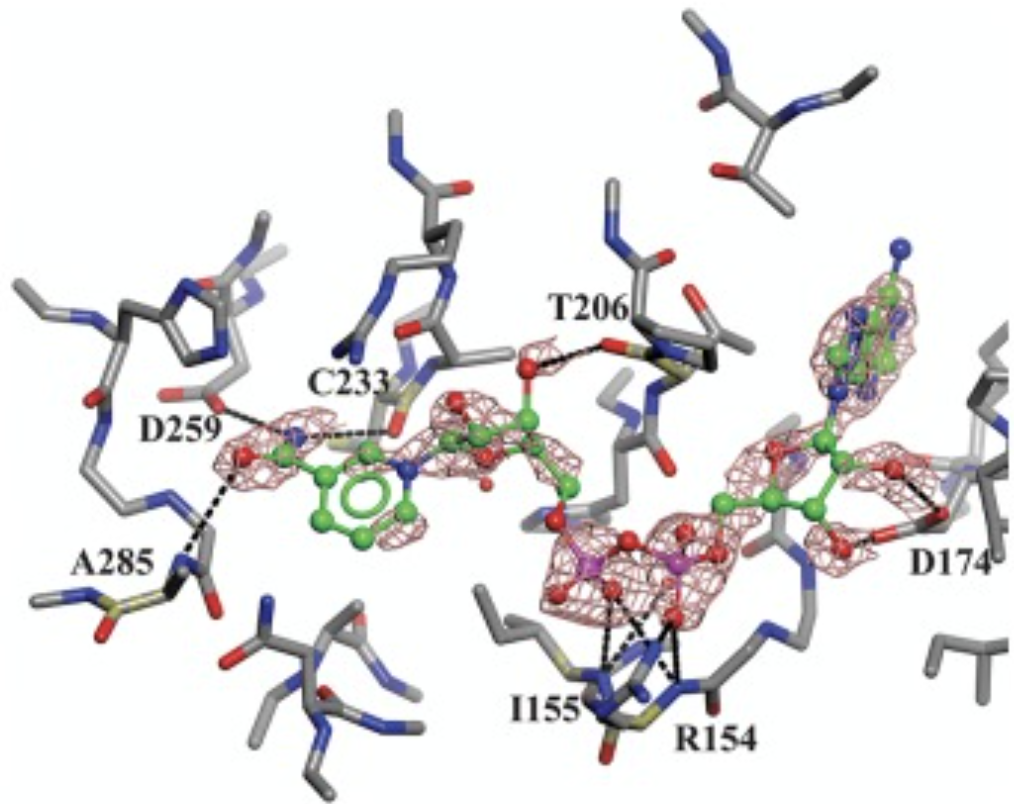
Figure 7: PHGDH with NAD binding site.

Appendix D Generated Molecules

We visualize a part of generated molecules from single and multi-objective optimization of ESR1, ACAA1, and PHGDH. Additionally, several conditionally generated C2 and C3, which have similar characteristics to human-designed ones, are also presented in Fig. 14 and Fig. 15.

D.1 Multi-Objective and Single-Objective Optimization

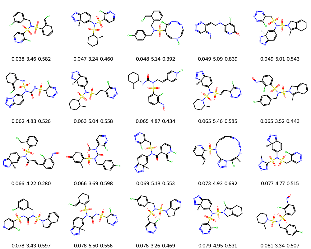
Figure 8: Molecules produced during the multi-objective optimization for ESR1. The legends denote ${K_{D}}\rm{(nM)}\downarrow$, SA$\downarrow$ and QED$\uparrow$.

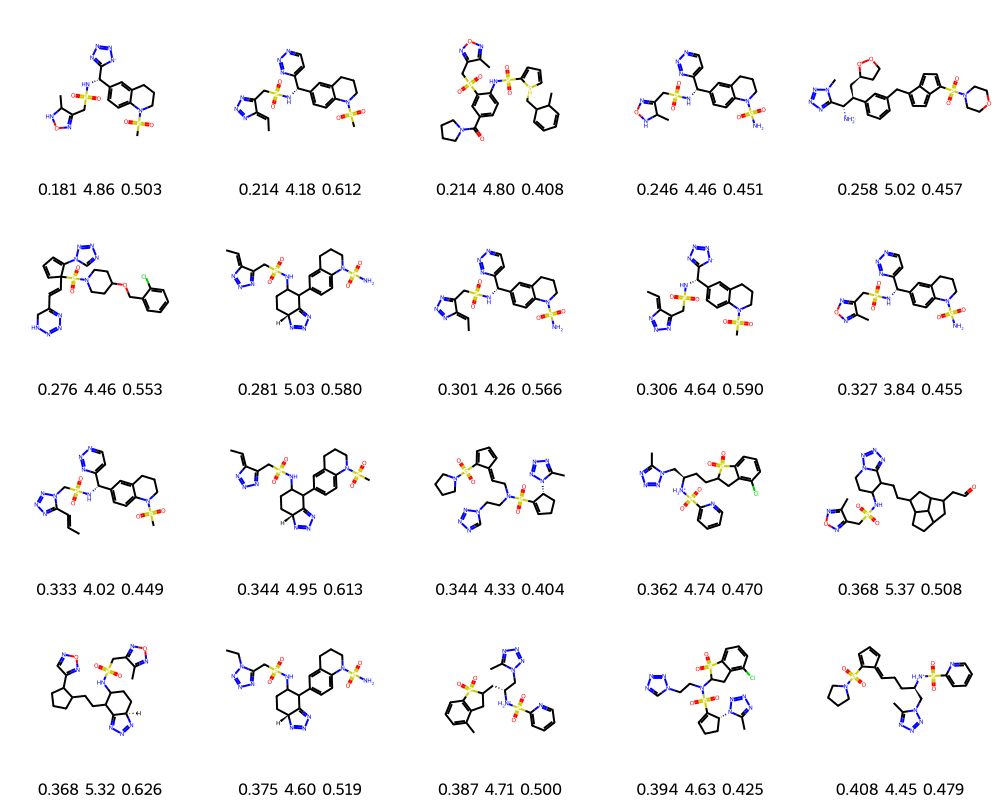
Figure 9: Molecules produced during the multi-objective optimization for ACAA1. The legends denote ${K_{D}}\rm{(nM)}\downarrow$, SA$\downarrow$ and QED$\uparrow$.

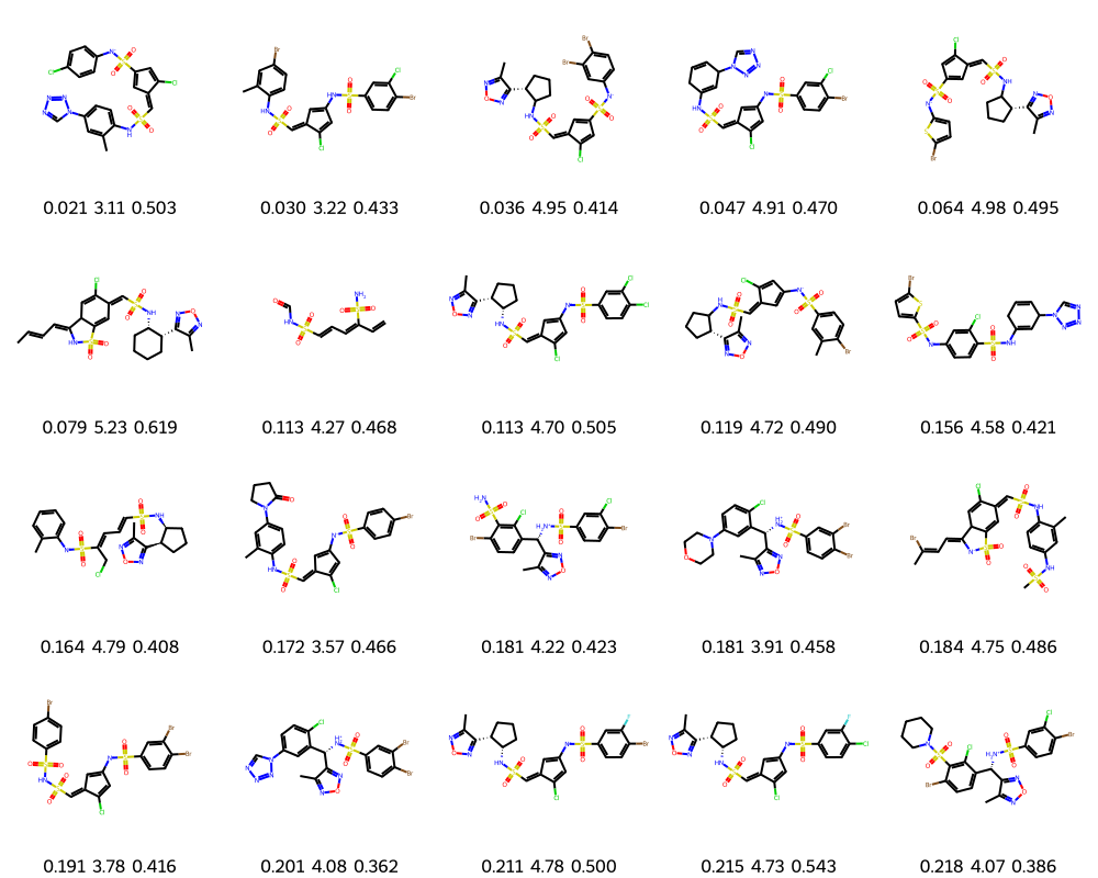
Figure 10: Molecules produced during the multi-objective optimization for PHGDH. The legends denote ${K_{D}}\rm{(nM)}\downarrow$, SA$\downarrow$ and QED$\uparrow$.

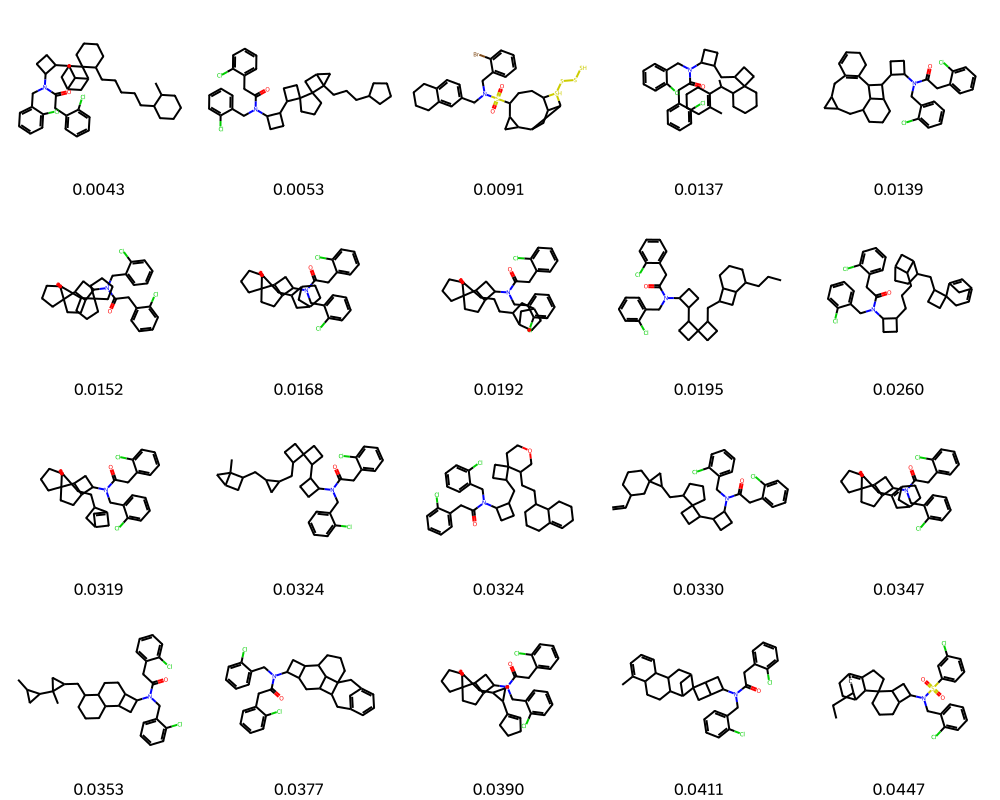
Figure 11: Molecules produced during the single-objective optimization for ESR1. The legends denote $\mathrm{K_{D}}(nM)\downarrow$.

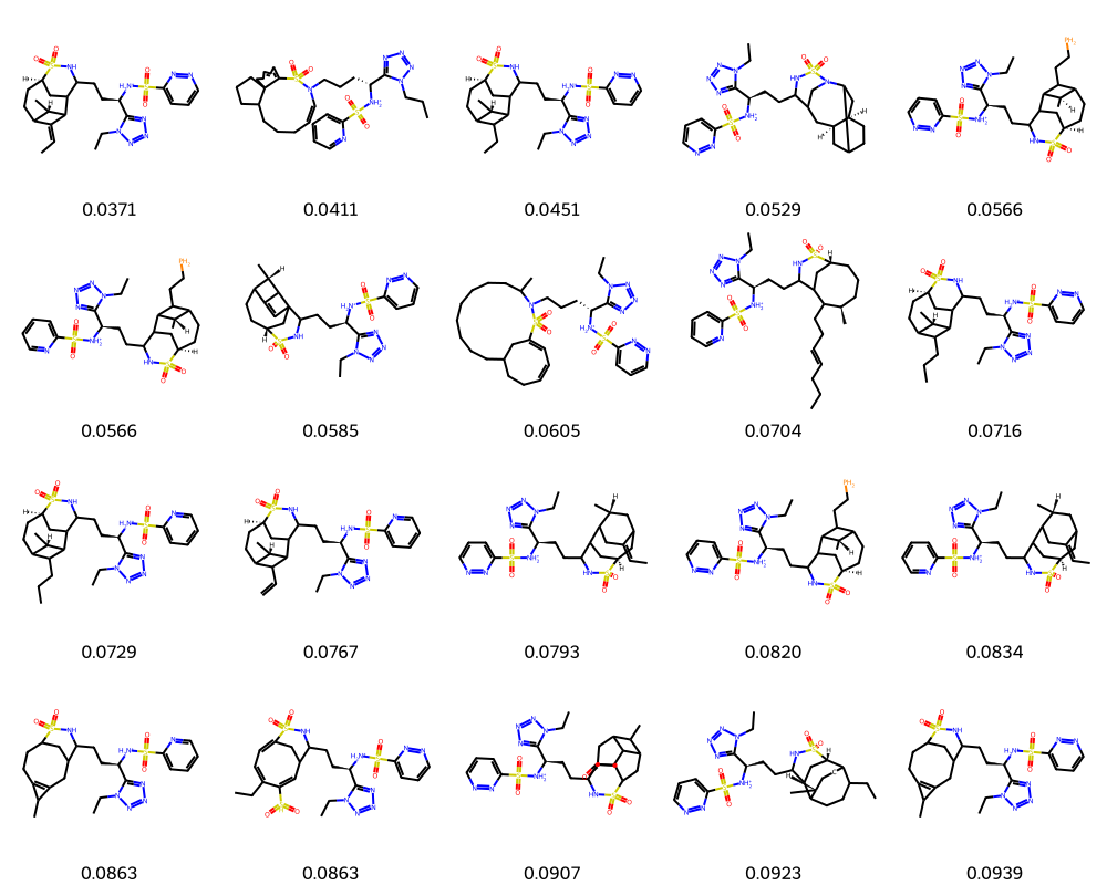
Figure 12: Molecules produced during the single-objective optimization for ACAA1. The legends denote $\mathrm{K_{D}}(nM)\downarrow$.

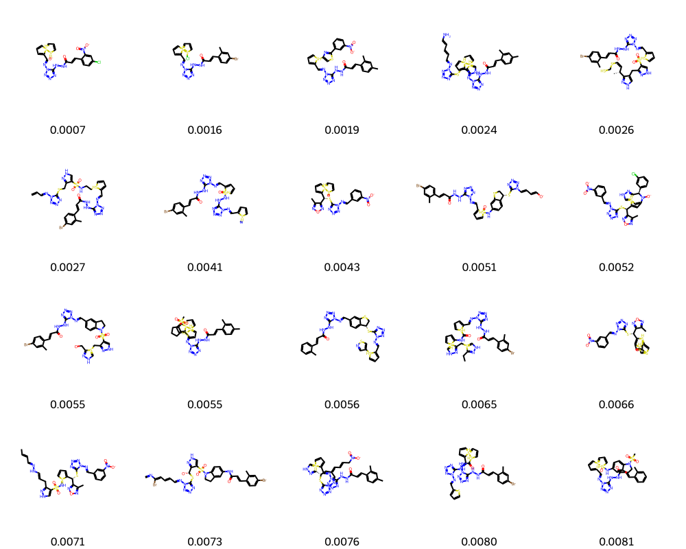
Figure 13: Molecules produced during the single-objective optimization for PHGDH. The legends denote $\mathrm{K_{D}}(nM)\downarrow$.

D.2 Structure-constrained Optimization

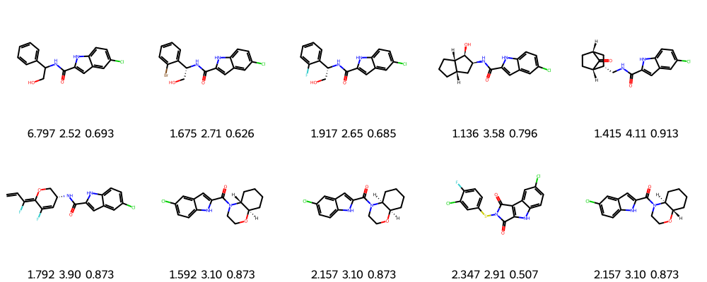
Figure 14: Molecules produced during the structure-constrained optimization from C1 to C2 for PHGDH. The legends denote $K_{D}\rm{(\mu M)}\downarrow$, SA$\downarrow$ and QED$\uparrow$.

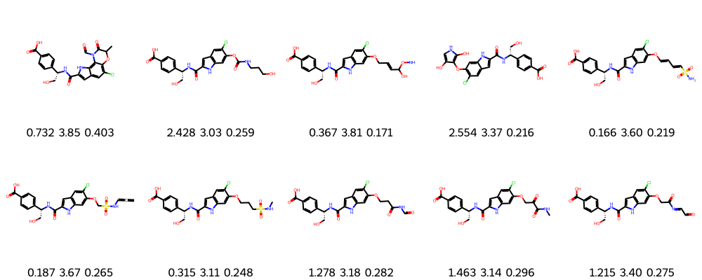
Figure 15: Molecules produced during the structure-constrained optimization from C2 to C3 for PHGDH. The legends denote $K_{D}\rm{(\mu M)}\downarrow$, SA$\downarrow$ and QED$\uparrow$.

References

- Brookes et al. (2019) Brookes, D., Park, H., and Listgarten, J. Conditioning by adaptive sampling for robust design. In International conference on machine learning (ICML), pp. 773–782. PMLR, 2019.
- Cheng et al. (2023) Cheng, A. H., Cai, A., Miret, S., Malkomes, G., Phielipp, M., and Aspuru-Guzik, A. Group selfies: a robust fragment-based molecular string representation. Digital Discovery, 2023.
- De Cao & Kipf (2018) De Cao, N. and Kipf, T. Molgan: An implicit generative model for small molecular graphs. arXiv preprint arXiv:1805.11973, 2018.
- Du et al. (2022) Du, Y., Fu, T., Sun, J., and Liu, S. Molgensurvey: A systematic survey in machine learning models for molecule design. arXiv preprint arXiv:2203.14500, 2022.
- Eckmann et al. (2022) Eckmann, P., Sun, K., Zhao, B., Feng, M., Gilson, M. K., and Yu, R. Limo: Latent inceptionism for targeted molecule generation. In International Conference on Machine Learning (ICML), 2022.
- Fannjiang & Listgarten (2020) Fannjiang, C. and Listgarten, J. Autofocused oracles for model-based design. Advances in Neural Information Processing Systems (NeurIPS), 33:12945–12956, 2020.
- Fu et al. (2021) Fu, T., Gao, W., Xiao, C., Yasonik, J., Coley, C. W., and Sun, J. Differentiable scaffolding tree for molecular optimization. arXiv preprint arXiv:2109.10469, 2021.
- Fuller et al. (2016) Fuller, N., Spadola, L., Cowen, S., Patel, J., Schönherr, H., Cao, Q., McKenzie, A., Edfeldt, F., Rabow, A., and Goodnow, R. An improved model for fragment-based lead generation at astrazeneca. Drug Discovery Today, 21(8):1272–1283, 2016.
- Gómez-Bombarelli et al. (2018) Gómez-Bombarelli, R., Wei, J. N., Duvenaud, D., Hernández-Lobato, J. M., Sánchez-Lengeling, B., Sheberla, D., Aguilera-Iparraguirre, J., Hirzel, T. D., Adams, R. P., and Aspuru-Guzik, A. Automatic chemical design using a data-driven continuous representation of molecules. ACS Central Science, 4(2):268–276, 2018.
- Hansen (2006) Hansen, N. The cma evolution strategy: a comparing review. Towards a new evolutionary computation: Advances in the estimation of distribution algorithms, pp. 75–102, 2006.
- Irwin et al. (2012) Irwin, J. J., Sterling, T., Mysinger, M. M., Bolstad, E. S., and Coleman, R. G. Zinc: a free tool to discover chemistry for biology. Journal of Chemical Information and Modeling, 52(7):1757–1768, 2012.
- Jain et al. (2022) Jain, M., Bengio, E., Hernandez-Garcia, A., Rector-Brooks, J., Dossou, B. F., Ekbote, C. A., Fu, J., Zhang, T., Kilgour, M., Zhang, D., et al. Biological sequence design with gflownets. In International Conference on Machine Learning (ICML), pp. 9786–9801. PMLR, 2022.
- Jin et al. (2018) Jin, W., Barzilay, R., and Jaakkola, T. Junction tree variational autoencoder for molecular graph generation. In International Conference on Machine Learning (ICML), pp. 2323–2332, 2018.
- Kingma & Ba (2014) Kingma, D. P. and Ba, J. Adam: A method for stochastic optimization. arXiv preprint arXiv:1412.6980, 2014.
- Kong et al. (2023) Kong, D., Pang, B., Han, T., and Wu, Y. N. Molecule design by latent space energy-based modeling and gradual distribution shifting. In Conference on Uncertainty in Artificial Intelligence (UAI), volume 216, pp. 1109–1120, 2023.
- Krenn et al. (2020) Krenn, M., Häse, F., Nigam, A., Friederich, P., and Aspuru-Guzik, A. Self-referencing embedded strings (selfies): A 100% robust molecular string representation. Machine Learning: Science and Technology, 1(4):045024, 2020.
- Kusner et al. (2017) Kusner, M. J., Paige, B., and Hernández-Lobato, J. M. Grammar variational autoencoder. In International Conference on Machine Learning (ICML), pp. 1945–1954, 2017.
- (18) Landrum, G. et al. RDKit: Open-source cheminformatics. URL https://www.rdkit.org.
- Loshchilov & Hutter (2019) Loshchilov, I. and Hutter, F. Decoupled weight decay regularization. In International Conference on Learning Representations (ICLR), 2019.
- Luo et al. (2021) Luo, Y., Yan, K., and Ji, S. Graphdf: A discrete flow model for molecular graph generation. In International Conference on Machine Learning (ICML), pp. 7192–7203, 2021.
- Mullarky et al. (2019) Mullarky, E., Xu, J., Robin, A. D., Huggins, D. J., Jennings, A., Noguchi, N., Olland, A., Lakshminarasimhan, D., Miller, M., Tomita, D., et al. Inhibition of 3-phosphoglycerate dehydrogenase (phgdh) by indole amides abrogates de novo serine synthesis in cancer cells. Bioorganic & medicinal chemistry letters, 29(17):2503–2510, 2019. URL https://www.ncbi.nlm.nih.gov/pmc/articles/PMC6702104/.
- Neal (2011) Neal, R. M. MCMC using hamiltonian dynamics. Handbook of Markov Chain Monte Carlo, 2, 2011.
- Nigam et al. (2020) Nigam, A., Friederich, P., Krenn, M., and Aspuru-Guzik, A. Augmenting genetic algorithms with deep neural networks for exploring the chemical space. In International Conference on Learning Representations (ICLR), 2020.
- Nijkamp et al. (2020) Nijkamp, E., Pang, B., Han, T., Zhou, L., Zhu, S.-C., and Wu, Y. N. Learning multi-layer latent variable model via variational optimization of short run mcmc for approximate inference. In European Conference on Computer Vision (ECCV), pp. 361–378, 2020.
- Pang et al. (2020) Pang, B., Han, T., Nijkamp, E., Zhu, S.-C., and Wu, Y. N. Learning latent space energy-based prior model. In Advances in Neural Information Processing Systems (NeurIPS), 2020.
- Ronneberger et al. (2015) Ronneberger, O., Fischer, P., and Brox, T. U-net: Convolutional networks for biomedical image segmentation. In Medical Image Computing and Computer-Assisted Intervention–MICCAI 2015: 18th International Conference, Munich, Germany, October 5-9, 2015, Proceedings, Part III 18, pp. 234–241. Springer, 2015.
- Samanta & Semenza (2016) Samanta, D. and Semenza, G. L. Serine synthesis helps hypoxic cancer stem cells regulate redox. Cancer research, 76(22):6458–6462, 2016. URL https://pubmed.ncbi.nlm.nih.gov/27811150/.
- Santos-Martins et al. (2021) Santos-Martins, D., Solis-Vasquez, L., Tillack, A. F., Sanner, M. F., Koch, A., and Forli, S. Accelerating AutoDock4 with GPUs and gradient-based local search. Journal of Chemical Theory and Computation, 17(2):1060–1073, 2021.
- Shi et al. (2020) Shi, C., Xu, M., Zhu, Z., Zhang, W., Zhang, M., and Tang, J. Graphaf: a flow-based autoregressive model for molecular graph generation. arXiv preprint arXiv:2001.09382, 2020.
- Spillier & Frédérick (2021) Spillier, Q. and Frédérick, R. Phosphoglycerate dehydrogenase (phgdh) inhibitors: A comprehensive review 2015–2020. Expert opinion on therapeutic patents, 31(7):597–608, 2021.
- Swersky et al. (2020) Swersky, K., Rubanova, Y., Dohan, D., and Murphy, K. Amortized bayesian optimization over discrete spaces. In Conference on Uncertainty in Artificial Intelligence (UAI), pp. 769–778. PMLR, 2020.
- Trabucco et al. (2021) Trabucco, B., Kumar, A., Geng, X., and Levine, S. Conservative objective models for effective offline model-based optimization. In International Conference on Machine Learning (ICML), pp. 10358–10368. PMLR, 2021.
- Trabucco et al. (2022) Trabucco, B., Geng, X., Kumar, A., and Levine, S. Design-bench: Benchmarks for data-driven offline model-based optimization. In International Conference on Machine Learning (ICML), pp. 21658–21676. PMLR, 2022.
- Unterlass et al. (2017) Unterlass, J. E., Wood, R. J., Baslé, A., Tucker, J., Cano, C., Noble, M. M., and Curtin, N. J. Structural insights into the enzymatic activity and potential substrate promiscuity of human 3-phosphoglycerate dehydrogenase (phgdh). Oncotarget, 8(61):104478, 2017. URL https://www.ncbi.nlm.nih.gov/pmc/articles/PMC5732821/.
- Weininger (1988) Weininger, D. Smiles, a chemical language and information system. 1. introduction to methodology and encoding rules. Journal of Chemical Information and Computer Sciences, 28(1):31–36, 1988.
- Wilson et al. (2017) Wilson, J. T., Moriconi, R., Hutter, F., and Deisenroth, M. P. The reparameterization trick for acquisition functions. CORR, abs/1712.00424, 2017. URL http://arxiv.org/abs/1712.00424.
- Winter et al. (2019) Winter, R., Montanari, F., Steffen, A., Briem, H., Noé, F., and Clevert, D.-A. Efficient multi-objective molecular optimization in a continuous latent space. Chemical Science, 10(34):8016–8024, 2019.
- Xie et al. (2019) Xie, J., Zhu, S., and Wu, Y. N. Learning energy-based spatial-temporal generative convnets for dynamic patterns. IEEE Transactions on Pattern Analysis and Machine Intelligence (TPAMI), abs/1909.11975, 2019. URL http://arxiv.org/abs/1909.11975.
- Xie et al. (2023) Xie, J., Zhu, Y., Xu, Y., Li, D., and Li, P. A tale of two latent flows: Learning latent space normalizing flow with short-run langevin flow for approximate inference. In Thirty-Seventh AAAI Conference on Artificial Intelligence, 2023.
- Xie et al. (2021) Xie, Y., Shi, C., Zhou, H., Yang, Y., Zhang, W., Yu, Y., and Li, L. Mars: Markov molecular sampling for multi-objective drug discovery. In International Conference on Learning Representations, 2021.
- Yang et al. (2020) Yang, X., Aasawat, T. K., and Yoshizoe, K. Practical massively parallel monte-carlo tree search applied to molecular design. arXiv preprint arXiv:2006.10504, 2020.
- You et al. (2018) You, J., Liu, B., Ying, Z., Pande, V., and Leskovec, J. Graph convolutional policy network for goal-directed molecular graph generation. In Advances in Neural Information Processing Systems (NeurIPS), pp. 6410–6421, 2018.
- Zhao et al. (2020) Zhao, X., Fu, J., Du, J., and Xu, W. The role of d-3-phosphoglycerate dehydrogenase in cancer. International Journal of Biological Sciences, 16(9):1495, 2020.
- Zhou et al. (2019) Zhou, Z., Kearnes, S., Li, L., Zare, R. N., and Riley, P. Optimization of molecules via deep reinforcement learning. Scientific Reports, 9(1):1–10, 2019.