Causal Orthogonalization: Multicollinearity, Economic Interpretability, and the Gram-Schmidt Process

Abstract

This paper considers the problem of interpreting orthogonalization model coefficients. We derive a causal economic interpretation of the Gram-Schmidt orthogonalization process and provide the conditions for its equivalence to total effects from a recursive Directed Acyclic Graph. We extend the Gram-Schmidt process to groups of simultaneous regressors common in economic data sets and derive its finite sample properties, finding its coefficients to be unbiased, stable, and more efficient than those from Ordinary Least Squares. Finally, we apply the estimator to childhood reading comprehension scores, controlling for such highly collinear characteristics as race, education, and income. The model expands Bohren et al.’s decomposition of systemic discrimination into channel-specific effects and improves its coefficient significance levels.

We are grateful to Anthony Nearman, Karen Rennick, Nathalie Steinhaur, and Dennis vanEnglesdorp for the initial motivation to solve the multicollinearity problem, W. Jason Beasley and Aaron Watt for early implementation and feedback, Peter Hull and J. Aislinn Bohren for their comments on discrimination decomposition in survey data, and Jennifer Alix-Garcia, David Kling, and David Lewis for comments on related research and project scope. Juan Carlos López-Morate suggested the exploration of and provided an excellent proof for the efficiency under included irrelevant variables property Theorem 2(G). [Name Surname; will be inserted later]

1 Introduction

Multicollinearity, or correlation among regressors, has posed a problem for statistical analysis since the introduction of Ordinary Least Squares (OLS) in 1805. Inflated standard errors depress statistical significance, and negative coefficient covariance renders models sensitive to small changes in regressor selection or functional form. A growing area of concern has been the emergence of p-hacking, the selection of regressors or functional forms to inflate statistical significance (Leamer, 1983; Gelman and Loken, 2014). The nearly structureless (empirical, ex-post) estimation approaches increasingly popular in applied research contribute to p-hacking’s allure. The statistical instability induced by any multicollinearity in the data will further exacerbate this influence on reported findings, as strategic or arbitrary replacement of one regressor with another can radically vary the conclusions. All this raises the stakes for discovering an alternative to OLS that will be both rationally interpretable and robust in the face of multicollinearity.

Various treatments for multicollinearity have been developed, each coming at some cost in terms of either coefficient bias or loss of interpretability. Step-wise methods (Hocking, 1976) and discretionary elimination of highly correlated regressors introduce omitted variable bias. The advantage of retaining all regressors via ridge regression (Hoerl and Kennard, 2000) comes at the cost of systematic downward bias.

Orthogonalization is a popular approach for applications such as computation, machine learning, and signal processing, where directly interpretable coefficients are not required (Greene, 2018; Despois and Doz, 2023). Laplace (1816) introduced his orthogonalization approach to compute Legendre’s newly popularized (1805) least-squares regression, free of Gauss’s (1809) computationally more expensive normal equations (see Stigler (1981). Laplace’s method was independently discovered by Gram (1883), Schmidt (1907), and Iwasawa (1949), and coined the Modified Gram-Schmidt Process by Wong (1935) (see Farebrother (1988)). The Gram-Schmidt is a special case of upper-triangular matrix decomposition, referred to by Francis (1961) as QR decomposition, which preserves all information in the original data set, a so-called lossless process.

Following Laplace, Pearson (1901) introduced Principal Component Analysis (PCA), another lossless decomposition approach popular for covariate-importance ranking. Partial Least Squares was introduced by Wold (1966) as a special case of Least Squares QR (Paige and Saunders, 1982) originally intended for forecasting highly collinear systems (see Wold et al., 1984). Finally, Singular Value Decomposition (SVD) (Golub and Reinsch, 1970) is a non-lossless, eigenvalue-based method popular for data compression.

The contribution of this paper is four-fold. First, we explore conditions for equivalence between the Gram-Schmidt process and Wold and Pearl’s recursive causal inference model, providing the first causally interpretable and lossless approach for removing multicollinearity. Second, we extend the Gram-Schmidt process to simultaneous regressors common in economic data sets, expanding the model’s use beyond strictly recursive regressors or causal chains. Third, we derive the finite sample properties of the Gram-Schmidt and extended Gram-Schmidt least-squares models. We show these models preserve all regressor information and that their coefficients are unbiased, stable, more efficient than OLS, and more robust to omitted variable bias and inclusion of irrelevant variables. Finally, we illustrate the extended model by replicating and extending the work of Lubotsky and Wittenberg (2006) and others, who assessed child reading and comprehension outcomes while controlling for several simultaneous groups of collinear household characteristics. Our results extend these earlier findings to the Bohren et al. (2023) decomposition, which breaks total discrimination down into its direct and systemic (intermediate) elements. We expand this decomposition further, showing how the extended model divides systemic discrimination into its channel-specific mechanisms, including education, income, and household formation.

Our interpretability result is motivated by earlier research in interdependent dynamic systems, first explored in the 1920s by economists interested in describing and forecasting simultaneous supply and demand relations. There, system identification was a primary focus. Early strategies included the instantaneous equilibrium condition, lagged endogenous variables, causal chains, and instrumental variables. Schultz (1928) introduced the cobweb model, extended by Wright (1925, 1934) to path analysis and instrumentation. Wold generalized these causal chain and dynamic system approaches to the Linear Systems of Equations Model (LSEM) (1951; 1960), showing in a time-series framework that model coefficients were asymptotically consistent (1963). Goldberger (1972) explored systems with unobservable regressors and early latent factor models. Alwin and Hauser (1975) first calculated indirect effects and their confidence intervals by using a product-of-coefficients method.

Rubin (1974) refocused causal identification away from LSEM’s lagged variables and instantaneous equilibria toward the random control trial (RCT) strategies inspired by Neyman (1923), the so-called Rubin causal model (see Holland, 1986), or Potential Outcomes approach (see Imbens, 2020). Imbens and Angrist (1994) and Card and Krueger (1994) expanded these strategies greatly, particularly the use of instrumental variables, difference-in-difference, and shape restrictions, frequently considering models with potential endogeneity from omitted variables. The resulting Causal Inference framework is used widely across academic disciplines.

Parallel to these efforts, Pearl (2000) expanded the graphical intuition of the LSEM to the Causal Mediation framework, of growing popularity in the biological, computer, and social sciences outside economics. He showed a regressor’s total effect to be a partial derivative of an independent variable with respect to the regressor’s path through a causal system, formalizing Wright’s (1934) method of path coefficients and extending Wold’s chain principle (1963) beyond a time series setting. Pearl recast Wold’s conditions in terms of Directed Acyclic Graphs (DAGs) or Bayesian Networks. One-way causality is achieved either when regressors are temporally separated from one another by the natural occurrence of the data or by experimental design, referred to as Sequential Ignorability. Pearl (2000, p. 418) shows Sequential Ignorability to be equivalent to the Gauss-Markov assumptions under the additional conditions of independent residual vectors and freedom from any heterogeneity induced by unobservable regressors. Simultaneous regressor models remain unidentified in the DAG framework.

This paper proceeds as follows. The following section introduces the Gram-Schmidt process for a simplified data set of two recursive regressors. Section 3 reviews recursive DAGs and the simultaneous regressor problem. Section 4 offers our main result - conditions under which Gram-Schmidt coefficients are equivalent in expected value to interpretable economic total effects, represented by a recursive DAG, and then derives their finite-sample estimation properties. Section 5 extends the Gram-Schmidt method to a mixed data set containing simultaneous as well as recursive regressors and derives the extended estimation properties. Section 6 illustrates the new model by replicating and expanding the work of Lubotsky and Wittenberg (2006) and others, who consider the effects of collinear family and individual characteristics on child reading and comprehension. Section 7 concludes.

2 The Gram-Schmidt Process

The Gram-Schmidt process begins with a data set $X$ consisting of $K$ real-valued variables arranged in random order. The second variable is regressed on the first and replaced with the resulting residual; then, the regression coefficient is saved. This process is repeated, each variable regressed successively on all prior and then replaced by the resulting residual, saving the coefficients. The outcome is an upper-triangular matrix of estimation coefficients $C$ and a new variable matrix $U$ constituting the orthogonal basis of the original data set, essentially preserving all variable information but in orthogonal form. The final step is to divide each residual by its standard deviation, creating the regressor set’s orthonormal basis. The latter step will be excluded below, although it is sometimes useful, and such coefficients can be interpreted in terms of standard-deviation units.

The Gram-Schmidt process can be represented by a set of line-by-line OLS regression equations, with each residual replaced by the prior equation’s residual. The simple recursive system represented in Figure 1(a) can be represented as follows:

$$x =u_{x},$$ (1)

$$z =c_{xz}u_{x}+u_{z},$$ (2)

$$y =c_{xy}u_{xy}+c_{zy}u_{z}+u_{y},$$ (3)

where $c_{xz}$, $c_{xy}$, and $c_{zy}$ are estimated coefficients, $x$, $z$, and $y$ are data vectors, and $u_{x}$, $u_{y}$, and $u_{z}$ the residuals. The coefficients can be specified as the inner-product ratios $c_{xz}=x^{\prime}z/x^{\prime}x$, where ^′ is the transpose operator.

In matrix form, the system including $y$ can be written as $X=U(C+I)$, where the $(K+1)\times N$ matrix $X=[x\;z\;y]$ is decomposed into three components: (i) the $(K+1)\times N$ matrix $U$, containing orthogonal residuals vectors $[u_{x}\;u_{z}\;u_{y}]$; (ii) the identity matrix $I$; and (iii) the upper-triangular $K\times K$ matrix

$$C=\begin{bmatrix}0&\hskip 8.5359ptc_{xz}&\hskip 8.5359ptc_{xy}\\ 0&\hskip 8.5359pt0&\hskip 8.5359ptc_{zy}\\ 0&\hskip 8.5359pt0&\hskip 8.5359pt0\end{bmatrix}$$ (4)

This procedure produces a convenient orthogonal data set $U$. But how can coefficient matrix $C$ be interpreted? To answer this, we next explore the recursive DAG model.

3 RECURSIVE DIRECTED ACYCLIC GRAPHS

DAG approaches typically involve formulating a structural system of equations, deriving the reduced form, and recovering the parameters once the system is identified. Three types of parameters are recovered in such systems: (i) direct effects, where a regressor acts, as is the case with OLS, directly on the dependent variable, holding other regressors constant; (ii) indirect effects, when a first regressor acts indirectly on the dependent variable by influencing a second regressor; and (iii) total effects, the sum of direct and indirect effects.

Figure 1 illustrates three basic causal systems: (i) the fully identified, recursive DAG; (ii) a system that is unidentified on account of an earlier-determined simultaneous regressor; and (iii) system (ii) but with a later-determined simultaneous regressor instead. Arrows indicate directions of causality of the recursive regressors $x$, $z$, and $y$, and simultaneous regressor $s$. The passage of time is shown on the far left.

(a) Recursive

(b) Early Simultaneous

(c) Late Simultaneous

Figure 1: Three causal directed-acyclic graphs.

To illustrate, consider the structural equations for the recursive example in Figure 1(a), where $x$ and $z$ are centered and ordered regressors; $y$ is the independent variable; $\beta_{ij}$, $i,j=x,z,y$, are the unobservable population parameters; and $\upsilon_{i}$ is the residual:

$$x =\upsilon_{x},$$ (5)

$$z =\beta_{xz}x+\upsilon_{z},$$ (6)

$$y =\beta_{xy}x+\beta_{zy}z+\upsilon_{y}.$$ (7)

Here, variables $x$ and $z$ are recursive because they occur one at a time in causal order by way of a temporal or experimentally designed separation. Specifically, $x$ is determined before $z$ and then affects $z$ directly through parameter $\beta_{xz}$. Regressor $x$ is also determined before y, acting upon $y$ directly through $\beta_{xy}$. Finally, $x$ exerts an indirect effect on $y$ by way of its influence on $z$, in turn influencing $y$ through $\beta_{zy}$. Together, the total effect of $x$ on $y$ is the sum of its direct and indirect effects, i.e., $(\beta_{xy}+\beta_{xz}\beta_{zy})$. By the chain rule, this total effect is also the partial derivative of $y$ with respect to $x$.

We can now assemble the total effects of the reduced form system, where residuals $\upsilon_{i}$, $i=x,z,y$ now serve as regressors:

$$x =\upsilon_{x},$$ (8)

$$z =\beta_{xz}\upsilon_{x}+\upsilon_{z},$$ (9)

$$y =(\beta_{xy}+\beta_{xz}\beta_{zy})\upsilon_{x}+\beta_{zy}\upsilon_{z}+\upsilon_{y}.$$ (10)

Note that parameter $\beta_{zy}$ is both the direct and total effect of $z$ on $y$, given that $z$ is the last regressor to be determined and influences no other regressors. This is also consistent with the Frisch-Waugh-Lovell decomposition theorem (Frisch and Waugh, 1933; Lovell, 1963), first described by Yule (1907), that $\beta_{zy}$ is recoverable from the regression of residual $\upsilon_{z}$ and $z$ on $y$.

The source of multicollinearity in this recursive system is that each regressor influences those determined later. For instance, when regressors are standardized and no spurious or incidental multicollinearity is present, the covariance between $x$ and $z$ is exactly the direct-effect parameter $\beta_{xz}$.

For convenience, the entire reduced-form system, including the dependent variable, can also be represented as a matrix decomposition $X=U(A+I)$, with upper-triangular parameter matrix:

$$A=\bNiceArray{ccc}[first-row,code-for-first-row=\scriptstyle]\\ 0&\hskip 14.22636pt\beta_{xz}\hskip 14.22636pt\beta_{xy}+\beta_{xz}\beta_{zy}\\ 0\hskip 14.22636pt0\hskip 14.22636pt\beta_{zy}\\ 0\hskip 14.22636pt0\hskip 14.22636pt0\\$$ (11)

Matrix $A$ also represents the matrix of first-order partial derivatives because $\tfrac{\partial y}{\partial x}=\beta_{xy}+\beta_{xz}\beta_{zy}$. The parameter matrix $A$ appears similar to the Gram-Schmidt coefficient matrix $C$, which we now formalize.

4 EQUIVALENCE AND ESTIMATION PROPERTIES

Under the following assumptions, an equivalence holds between Gram-Schmidt coefficients $c_{ij}\in C$ in (4), $i,j=1,...,K$, and the reduced-form DAG parameters $a_{ij}\in A$ in (11):

1. $X\subseteq\mathcal{R}^{[N\times K]}$ is a full-rank, ordered regressor matrix including dependent variable $y=x_{K}$;

2. $X$ has positive degrees of freedom $N>K$; and

3. the error vectors have zero conditional means: $E[\upsilon_{i}|x_{j}]=0$, $j=1,...,i-1$.

We will denote the sample residual vectors as $u_{i}\subseteq U$, $i=1,...,K$.

Theorem 1 (Equivalence).

Under assumptions (a) - (c), there exists a unique Gram-Schmidt coefficient matrix $C\subseteq\mathcal{R}^{[K\times K]}$ equivalent in expectation to the recursive DAG reduced-form matrix $A\subseteq\mathcal{R}^{[K\times K]}$:

$$E[C]=A.$$ (12)

A proof is provided in the Appendix.

For comparison with our current example, define the OLS estimation model of equation (7) as

$$y=b_{xy}x+b_{zy}z+u_{y}.$$ (13)

In the next theorem, we will compare the finite sample properties of Gram-Schmidt coefficients $c_{ij}$ in equations (1) - (3) with those of the OLS-estimated $b_{ij}$ in equation (13).

Define: (i) $X_{-j}$ as the full regressor set $X$ excluding regressor $x_{j}$; (ii) $X_{+k}$ as the regressor set including the additional variable $x_{k}$; (iii) $X_{<j}$ as the regressor set including ordered regressors $x_{i}$ up to, but not including, $x_{j}$, $i=1,...,j-1$; and (iv) $R_{jX_{<j}}^{2}$ as the coefficient of determination of the regression of $x_{j}$ on the set of remaining regressors $X_{<j}$. We will assume the regressor order is $i<k<j$ throughout, in which $x_{j}$ will be the $j^{\text{th}}$ equation’s dependent variable. We make one additional assumption:

1. OLS and Gram-Schmidt residuals $\upsilon_{i}$ are free of autocorrelation and heteroscedasticity, $E[\upsilon_{i}\upsilon_{i}^{\prime}|\mathbf{X}]=\sigma_{i}^{2}\mathbf{I}$.

Theorem 2 (Properties).

Under assumptions (a) - (d), the Gram-Schmidt system $X=U(C+I)$ in equations (1) - (3) obtains the following estimation properties:

(A)	Regressors are orthogonal, $u_{i}\perp u_{j}$;
(B)	Coefficients are stable, $Cov[c_{ij},c_{ji}]=0$;
(C)	Coefficients are unbiased, $E[c_{ij}]=a_{ij}$;
(D)	All information is preserved, $R_{j\,X_{<j}}^{2}=R_{j\,U_{<j}}^{2}$;
(E)	Omitted variable bias is zero, $E[c_{ij}|X]=E[c_{ij}|X_{-k}]$;
(F)	Gram-Schmidt is more efficient than OLS, $V[c_{ij}]\leq V[b_{ij}]$; and
(G)	Gram-Schmidt is more efficient than OLS under included irrelevant variables,
	$V[c_{ij}|X_{+k}]\leq V[b_{ij}|X_{+k}]$.

Proofs are provided in the Appendix.

Confidence intervals of the total effects and model inference are obtained directly from the terminal Gram-Schmidt regression, eliminating the need to reconstruct indirect effects by way of either product-of-coefficients (Alwin and Hauser (1975)) or simulation methods.

5 EXTENDED GRAM-SCHMIDT LEAST SQUARES

The Gram-Schmidt transformation is equivalent to the recursive DAG when every regressor is recursive, that is, strictly separated by time or when the experimental design is such that no feedback can occur between regressors. However, the latter is an unlikely condition in practice because regressor simultaneity is present in many naturally occurring – and even some experimentally designed – data sets, especially when data collection intervals are wide. In the present section, we extend the Gram-Schmidt process to allow a block of simultaneous regressors to replace a single recursive regressor. This preserves temporal ordering but avoids endogeneity bias because the simultaneous regressors within a block are not regressed on one another. Instead, we construct a block-upper-triangular system of coefficients, the final column representing the total effects on the dependent variable from the relevant regressor. Coefficients thus remain consistent with the dependent variable’s partial derivatives with respect to the relevant regressor’s path-specific effect described by Pearl (2000), excluding feedback effects. By omitting only the mutual regressions of the simultaneous regressors, we allow the recovered total effects to exclude only direct feedback effects among simultaneous regressors. Indirect effects of such feedback that may progress through the system are preserved in the total effects of earlier-occurring regressors.

5.1 Simultaneous Regressors

It is worthwhile first to explore the identification problem raised by these simultaneous regressors. It is well known that simultaneous equations, such as supply and demand systems, are not directly identifiable, so parameters cannot be immediately recovered. The same is true for simultaneous regressors in structural or DAG models. Consider then a simplified system with two simultaneous regressors $s$ and $x$:

$$s =\beta_{xs}x+\upsilon_{s},$$ (14)

$$x =\beta_{sx}s+\upsilon_{x},$$ (15)

$$y =\beta_{sy}s+\beta_{xy}x+\upsilon_{y}.$$ (16)

This system is unidentified because neither the simultaneous coefficients nor the residual vectors are observable.

Partial derivatives can, however, be obtained by way of the Implicit Function Theorem:

$$\frac{\partial y}{\partial x}=\beta_{xy}+\beta_{sy}\frac{1+\beta_{xs}}{1+\beta_{sx}}.$$

Unfortunately, the partial derivatives here are also functions of the unrecoverable parameters $\beta_{sx}$ and $\beta_{xs}$. We will refer to these unrecoverable parameters as feedback effects. Direct effects $\beta_{iy}$ are however fully recoverable because OLS remains unbiased, $E[b_{iy}]=\beta_{iy}$. We will also find a way to recover some feedback information from earlier-occurring regressors.

Multicollinearity is assured by the simultaneity of $x$ and $s$, illustrated by the off-diagonal elements of the variance-covariance matrix $\Sigma_{s}$ of the standardized regressors, shown here without the influence of additional spurious or incidental multicollinearity:

$$\Sigma_{s}=\bNiceArray{cc}[first-row,code-for-first-row=\scriptstyle]\\ \frac{1+\beta_{xs}^{2}}{(1-\beta_{xs}\beta_{sx})^{2}}&\hskip 8.5359pt\frac{\beta_{xs}+\beta_{sx}}{(1-\beta_{xs}\beta_{sx})^{2}}\\ \frac{\beta_{xs}+\beta_{sx}}{(1-\beta_{xs}\beta_{sx})^{2}}\hskip 8.5359pt\frac{1+\beta_{sx}^{2}}{(1-\beta_{xs}\beta_{sx})^{2}}\\$$ (17)

In the next section, we explore the information that can be recovered when a system contains both simultaneous and recursive regressors.

5.2 Mixed Simultaneous and Recursive Regressors

Consider next a system containing both an earlier- and later-determined simultaneous regressor block as illustrated in Figures 1(b) and 1(c), respectively. We will motivate the problem for the earlier-determined simultaneous block case, Fig 1(b), although the properties of the extended method shown here apply to both cases.

The structural equations assumed in Fig 1(b) are:

$$s =\beta_{xs}x+\upsilon_{s},$$

$$x =\beta_{sx}s+\upsilon_{x},$$

$$z =\beta_{sz}s+\beta_{xz}x+\upsilon_{z},$$

$$y =\beta_{sy}s+\beta_{xy}x+\beta_{zy}z+\upsilon_{y}.$$

As in our simultaneity example in subsection 5.1 above, $s$ and $x$ here are simultaneous. But $z$ has replaced $y$ as the third regressor in the simultaneous system (14)-(16), so dependent variable $y$ is now a function of three regressors. We know direct feedback effects are unrecoverable, while direct effects $\beta_{iz}$ and $\beta_{iy}$ are recoverable, though OLS will suffer from steep multicollinearity. This can be seen in the covariance between $s$ and $z$, illustrated in the following equation for standardized regressors with no additional spurious multicollinearity:

$$Cov[s,z] =\frac{\beta_{sz}(1+\beta_{xs}^{2})+\beta_{xz}(\beta_{xs}+\beta_{sx})}{(1-\beta_{xs}\beta_{sx})^{2}}.$$

As explored next, it will be possible to recover more information than direct effects alone and continue to remove the recursive portion of the multicollinearity.

5.3 The Gram-Schmidt Extension

Our first step is to derive the reduced-form equations in terms of the recursive residual $\upsilon_{z}$ – along with simultaneous regressors $x$ and $s$ – rather than in terms of the residuals as was the case for $x$ and $z$ in the original Gram-Schmidt model (8)-(10):

$$s =s,$$

$$x =x,$$

$$z =\beta_{sz}s+\beta_{xz}x+\upsilon_{z},$$

$$y =(\beta_{sy}+\beta_{sz}\beta_{zy})s+(\beta_{xy}+\beta_{xz}\beta_{zy})x+\beta_{zy}\upsilon_{z}+\upsilon_{y}.$$

This system can be specified as $X=U(A+I)$, where $U=[s\>x\>\upsilon_{z}\upsilon_{y}]$ and parameter matrix $A$ – extending (11) – is now the block-upper-triangular partial derivatives matrix:

$$A=\bNiceArray{cccc}[first-row,code-for-first-row=\scriptstyle]\\ 0&\hskip 14.22636pt0\hskip 14.22636pt\beta_{sz}\hskip 14.22636pt\beta_{sy}+\beta_{sz}\beta_{zy}\\ 0\hskip 14.22636pt0\hskip 14.22636pt\beta_{xz}\hskip 14.22636pt\beta_{xy}+\beta_{xz}\beta_{zy}\\ 0\hskip 14.22636pt0\hskip 14.22636pt0\hskip 14.22636pt\beta_{zy}\\ 0\hskip 14.22636pt0\hskip 14.22636pt0\hskip 14.22636pt0$$ (18)

The extended method is then estimated as:

$$\negthickspace\begin{rcases}s=s\\ x=x\end{rcases}\textit{ Block 1,}$$

$$\negthickspace\begin{rcases}z=c_{sz}s+c_{xz}x+u_{z}\end{rcases}\textit{ Block 2,}$$

$$\negthickspace\begin{rcases}y=c_{sy}s+c_{xy}x+c_{zy}u_{z}+u_{y}\end{rcases}\textit{ Block 3.}$$

Block 1 consists of the early simultaneous regressors $x$ and $s$, as in Figure 1(b), while blocks 2 and 3 contain only one dependent variable, similar to the recursive case in Figure 1(a). Block 1 feedback coefficients $b_{sx}$ and $b_{xs}$ are omitted, so $x$ and $s$ are not regressed on one another. However, each dependent variable in blocks 2 and 3 is regressed on all regressors in the blocks previous to it so the indirect effects $b_{sz}$ and $b_{xz}$ are recovered.

Residual regressor matrix $U$ is no longer completely orthogonal. Rather, our extended method removes all covariance between any two blocks, in the present case between the simultaneous and recursive blocks, such that (i) the off-diagonal elements of the mixed variance-covariance partitioned matrix $\Sigma_{sr}$ are zero, for instance $Cov[s,u_{z}]=0$; but (ii) the simultaneous covariance matrix $\Sigma_{s}$ from equation (17) remains in the upper left:

$$\Sigma_{sr}=\left[\begin{array}[]{cc|c}\Sigma_{s}&&\hskip 5.69046pt\makebox{\text{\large 0}}\\ \hline\cr\makebox{\text{\large 0}}&&\hskip 5.69046pt1\end{array}\right],$$

where 0 is a conforming ($2\times 1$) zeros vector.

The extended method works similarly when a simultaneous regressor block follows a recursive regressor, as in Figure 1(c):

$$\negthickspace\begin{rcases}x=x\end{rcases}\textit{ Block 1,}$$

$$\negthickspace\begin{rcases}s=c_{xs}x+u_{s}\\ z=c_{xz}x+u_{z}\end{rcases}\textit{ Block 2,}$$

$$\negthickspace\begin{rcases}y=c_{xy}x+c_{sy}u_{s}+c_{zy}u_{z}+u_{y}\end{rcases}\textit{ Block 3.}$$

Block 2 now contains the two simultaneous regressors $s$ and $z$ in Figure 1(c) that will not be regressed on one another, although each will be regressed on $x$ in block 1. Covariances between pairs of blocks are again removed in the mixed variance-covariance partitioned matrix $\Sigma_{rs}$. For instance $Cov[u_{s},u_{z}]=0$ and the simultaneous covariance matrix $\Sigma_{s}$ shifts to the lower right:

$$\Sigma_{rs}=\left[\begin{array}[]{ccc|c}1&&&\hskip 2.84544pt\makebox{\text{\large 0}}\\ \hline\cr\makebox{\text{\large 0}}&&&\hskip 2.84544pt\Sigma_{s}\end{array}\right].$$

5.4 Extended Estimation Properties

We can now state the properties of our extended Gram-Schmidt least-squares (GSLS) method, which achieves the Theorem 2 properties across blocks rather than across individual regressors. Multicollinearity is eliminated from the recursive regressors, and recursive total effects are recovered. Multicollinearity among simultaneous regressors in a given block will be reduced but not eliminated. Feedback effects recovered, but the direct and intermediate effects are included in the simultaneous regressors’ total effects.

To show this, we revise the orthogonality assumption (a) in Theorems 1 and 2. Let $X\subseteq\mathcal{R}^{[N\times K]}$ be a full-rank matrix of recursively ordered regressor blocks $m,n,h=1,...M$, each block $m$ containing one or more regressors with coefficient $c_{i(m)j(n)}$, and block $m$ determined prior to block $n$, $m<n$. Throughout, we assume the regressor order to be $i<k<j$ and the block order to be $m<h<n$, with $x_{j(n)}$ the $j^{\text{th}}$ equation’s dependent variable.

With this revision in mind, we can summarize the properties of the GSLS estimator.

Theorem 3 (Properties).

Under our revised assumptions (a) - (d) above, the GSLS system $X=U(C+I)$ obtains the following estimation properties:

(A)	Regressors are orthogonal across blocks, $u_{i(m)}\perp u_{j(n)}$;
(B)	Coefficients are stable across blocks, $Cov[c_{i(m)j(n)},c_{k(h)j(n)}]=0$;
(C)	Coefficients are unbiased, $E[c_{i(m)j(n)}]=a_{i(m)j(n)}$;
(D)	All information is preserved, $R_{j(n)\,X_{<j(n)}}^{2}=R_{j(n)\,U_{<j(n)}}^{2}$;
(E)	Omitted variable bias is zero, $E[c_{i(m)j(n)}|X]=E[c_{i(m)j(n)}|X_{-k(h)}]$;
(F)	GSLS is more efficient than OLS, $V[c_{i(m)j(n)}]\leq V[b_{i(m)j(n)}]$; and
(G)	GSLS is more efficient than OLS under included irrelevant variables,
	$V[c_{i(m)j(n)}|X_{+k(h)}]\leq V[b_{i(m)j(n)}|X_{+k(h)}]$.

Proofs are provided in the Appendix.

6 EMPIRICAL APPLICATION

We now compare the GSLS estimator to OLS using data from the Bureau of Labor Statistics’ (2016) National Longitudinal Survey of Youth (NLSY). This data has been used by several researchers (Korenman et al., 1995; Blau, 1999; Lubotsky and Wittenberg, 2006) to explore the role of parental income on child reading comprehension test scores while controlling for several strongly interrelated individual and household characteristics. All three studies cite multicollinearity as a leading motivation of their model design, regressor selection, and interpretation of results. All three include both recursive and simultaneous regressors in their analysis. Readers may replicate the plots and analysis here with software packages available for R and Stata along with the NLSY data set (Cross (2024)).

The NLSY began as a survey of 6,283 women and 6,403 men aged 14 to 21 in 1979 and includes a wide range of characteristics, including employment, income, drug use, marriage, education, cognitive assessments, and childbirth. The sample was rebalanced in 1984 to exclude women serving in the military and again in 1990 and 1991 to correct for the survey’s original over-weighting of low-income white women. We will test for any remaining sample selection bias at the end of this section. Sampling frequency in the survey was annual through 1994 and biennial thereafter. A second survey, the Child Supplement, was initiated in 1986 to study the children of women included in the 1979 NLSY cohort, biennially recording cognitive achievement and behavior.

Childhood cognitive development is drawn from the Peabody Reading Comprehension Test. From 1986 to 2014, we include all complete observations of children aged 6-14 who were attempting the test for the first time. We exclude children of mothers dropped from the survey during the 1984, 1990, and 1991 revisions. The final sample includes, from the original NLSY cohort, 6,550 children born to 3,181 mothers.

Table 1: Summary statistics of NLSY data.

	Higher income		Lower income
	Mean	Std. dev.	Mean	Std. dev.
Black (proportion)	$17$%	$0.4$	$45$%	$0.5$
White (proportion)	$64$%	$0.5$	$31$%	$0.5$
Mother’s age	$35.1$	$5.9$	$31.8$	$5.7$
Mother’s education	$13.6$	$3.2$	$11.6$	$2.6$
Mother’s AFQT (percentile)	$48.2$	$27.0$	$23.0$	$21.0$
Spouse present (proportion)	$91$%	$1.3$	$33$%	$0.5$
Spouse’s age	$34.3$	$6.8$	$37.0$	$6.3$
Spouse’s education	$12.2$	$7.9$	$13.7$	$3.7$
Child female (proportion)	$49$%	$0.5$	$49$%	$0.5$
Child’s age	$7.6$	$1.4$	$8.0$	$1.6$
Family size	$4.5$	$1.2$	$4.2$	$1.7$
Family income ($\$$10K)	$12.3$	$14.7$	$2.6$	$1.3$
Child’s test score (percentile)	$63.9$	$24.1$	$51.7$	$26.4$

Table 1 summarizes the NLSY data by child, broken out into above- and below-median family income levels. Several regressor means and standard deviations differ materially between the high- and low-income groups, suggesting the 1984, 1990, and 1991 NLSY rebalancing efforts were insufficient or did not target income specifically. In the Covariate Matching subsection below we test for any remaining influence of sample selection bias.

Consistent with all three prior studies of these data, we include annual fixed effects and recursive regressors recorded on the date of test: child’s gender and age; logs of family size and income, and mother’s race, age, education, and performance on the 1980 Armed Forces Qualification Test (AFQT), a general knowledge exam administered to all participants in the original NLSY cohort. We also control for spousal presence in the household and spousal age and education to compare results with Lubotsky and Wittenberg (2006). Three simultaneous blocks are specified: (i) annual fixed effects; (ii) mother’s race, consisting of an indicator variable for black and for Hispanic (white the omitted variable); and (iii) spousal characteristics, including spouse’s residence in the home. All factors are specified in the natural temporal order in which they are assumed to have been determined. For instance, the child’s race is defined in the Child Supplement to be the mother’s race originally reported in the NLSY. Race was predetermined at the time of the mother’s conception, so precedes the mother’s age. In turn, both the mother’s race and age were determined before her highest grade level was achieved or her AFQT score was recorded. Spousal characteristics, child age and gender, and family size and income are all recorded when the child attempts the reading and comprehension test for the first time, so may influence the child’s test score, but cannot be influenced by it.

6.1 Results

Table 2 compares, for selected regressors, the OLS direct effects with GSLS total effects, including standard errors.

Table 2: Direct and Total Effects of Selected Regressors on Child’s Reading Scores.

	OLS direct effects		GSLS total effects
	Coeff.	S.E.	Coeff.	S.E.
Hispanic	$-0.40$	$(0.79)$	$-9.99$	$(0.72)$
Black	$-0.42$	$(0.78)$	$-11.06$	$(0.64)$
Mother’s age	$0.06$	$(0.14)$	$0.01$	$(0.13)$
Mother’s education	$0.41$	$(0.11)$	$1.83$	$(0.09)$
Mother’s AFQT	$0.21$	$(0.01)$	$0.29$	$(0.01)$
Spouse present	$1.86$	$(2.53)$	$1.36$	$(2.51)$
Child female	$5.46$	$(0.55)$	$6.49$	$(0.55)$
Child’s age	$-5.67$	$(0.19)$	$-5.75$	$(0.19)$
Family size (log)	$-8.38$	$(0.89)$	$-8.29$	$(0.89)$
Family income (log)	$1.37$	$(0.37)$	$1.37$	$(0.37)$
$R^{2}$	0.28		0.28

In both interpretation and expected value, GSLS coefficients differ from OLS in a meaningful way. OLS remains unbiased, $E[b_{xy}]=\beta_{xy}$, in the presence of multicollinearity, and its estimates of structural equation (7) represent direct effects. Coefficients are interpreted in the familiar way, namely as an increase or decrease in $y$ resulting from a unit increase in $x$, ceteris paribus, assuming all other regressors are fixed or independent. In linear models, this is the partial derivative of $y$ with respect to $x$, ignoring the regressor interrelatedness that induces multicollinearity. Intuitively, any such violation of the independence assumption confounds OLS inference and coefficient stability.

GSLS estimates the total effect, namely the total unit increase (decrease) in $y$ induced by a one-unit increase in $x$, including any indirect effects on $y$ induced or caused by changes the remaining $x$-dependent regressors. The latter, by the chain rule, is the partial derivative of $y$ with respect to $x$ given all structural relationships in equations (5) - (7), what Pearl refers to as path-switching (2001) or the path-specific effect (2000). GSLS significance levels are free from the influence of multicollinearity.

6.2 Family Income

Income’s estimated direct effect in the Table 2 OLS model is identical to its total effect in the GSLS model because income is the final causally-determined regressor in the model order. The 1.37 coefficient implies a one-percent income rise boosts relative reading comprehension by 1.37 percentile points and is similar to that reported by Blau (1999) and Lubotsky and Wittenberg (2006).

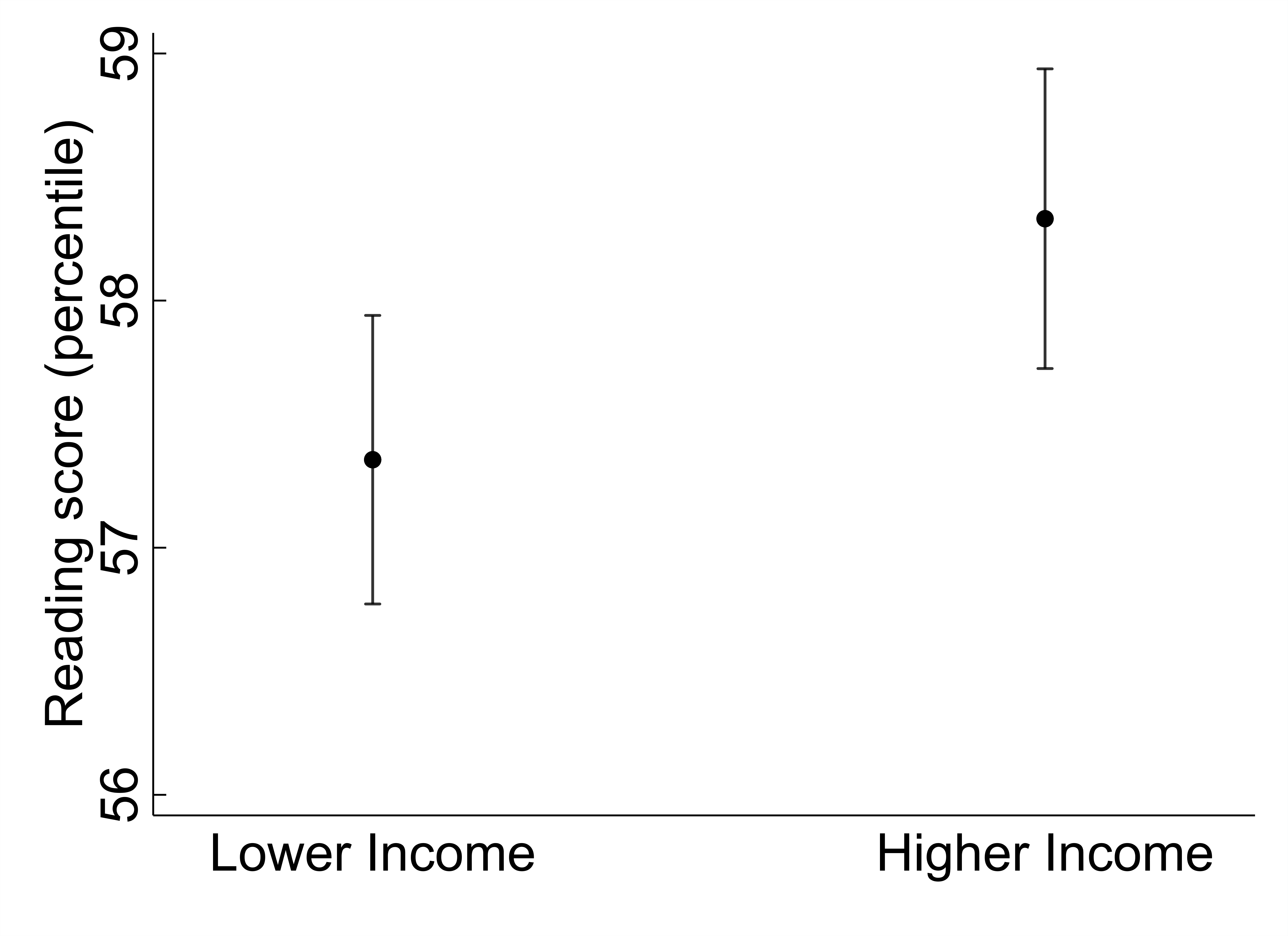
Figure 2: Family income effect on child reading and comprehension test score.

Figure 2 illustrates the GSLS estimates of income’s influence on a child’s reading score at the first and fourth quartile limits, respectively -0.32 and 0.39 of centered log income. Predicted test scores in the higher-income group are 1.12 percentage points greater than those in the lower group. This difference between the two quartile limits in income’s influence on reading comprehension is not significant at the 95% confidence level. However, it is significant over the full income range as shown in Table 2.

6.3 Race

Consistent with Blau (1999), the OLS estimate suggests no significant direct influence of maternal race on child test scores, indicated in the left-most column of Table 2. The GSLS model shows race’s total effect reduced reading scores by 10 percentile points among Hispanic children, relative to white, significant at the 99.9% confidence level. GSLS standard errors are lower than those in OLS by 9% and 18% among Hispanic and black children, respectively, illustrating the impacts of removing multicollinearity.

To understand the large rise in GSLS coefficient magnitudes, we look to the discrimination decomposition framework of Bohren et al. (2023). They define the total expected discrimination function $\Delta(y^{0})$ as the sum of direct and systemic discrimination:

$$\Delta(y^{0}) =\bar{\tau}(w,y^{0})+\delta(b,y^{0}),$$

where $b$ and $w$ are groups and $y^{0}$ is the unobservable initial qualification. The direct and systemic components here can be expressed in terms of expected values:

$$\bar{\tau}(w,y^{0})\hskip 5.69046pt =\hskip 5.69046ptE[A(w;\hskip 2.84544ptS_{i})\hskip 2.84544pt-\hskip 2.84544ptA(b;\hskip 2.84544ptS_{i})|G_{i}=w;\hskip 2.84544ptY^{0}_{i}=y^{0}],$$ (19)

$$\delta(b,y^{0})\hskip 5.69046pt =\hskip 5.69046ptE[A(b;\hskip 2.84544ptS_{i})|G_{i}=w;\hskip 2.84544ptY^{0}_{i}=y^{0}]\hskip 2.84544pt-\hskip 2.84544ptE[A(b;\hskip 2.84544ptS_{i})|G_{i}=b;\hskip 2.84544ptY^{0}_{i}=y^{0}].$$ (20)

Here, $A()$ is the action function, in our case the reading score function; $S_{i}$ is the set of signals for individual $i$, in our case the child’s racial and household background; $G_{i}$ is the set of groups ${w,b}$; and $Y^{0}_{i}$ is the set of initial qualifications, which we assume is equal across all children in the study since it represents their potential for reading before they are born.

In words, direct discrimination in (19) is the difference in action A, the test score, received by individual $i$, were they to belong to group $w$ rather than group $b$, holding the individual’s other signals (background characteristics) $S_{i}$ and initial qualification $y^{0}$ constant at group-$w$ level. This matches the interpretation shown in Table 2 of the OLS regression of test scores on race and other characteristics. Indeed, we find no evidence of direct discrimination, represented by the two nonsignificant coefficients for Hispanic and black children. This would be expected if test administration and scoring mechanisms did not differ systematically between groups.

Systemic discrimination in (20) is the expected difference between the score of a child from group $b$ but with background characteristics typical of group $w$, and the same child’s score given group $b$ background characteristics. It represents the cumulative effects of differences in access to such resources as education and employment opportunities, which Bohren et al. categorize as technological sources.

We can use GSLS to further decompose the systemic effect into its channel-specific mechanisms. Table 3 provides the intermediate-stage GSLS regression results for selected regressors. Race’s total effect on education can be seen in the second estimates column showing the regression of maternal school-grade completion on maternal race and age. Here, the total Hispanic effect on education was 1.31 fewer grades completed by an Hispanic mother than a white mother. In turn, each additional grade completed by the mother raised the child’s test score by 1.83 percentile points, as indicated in the last column of Table 3. Thus, we have a 2.4 percentile point (1.31 $\times$ 1.83) differential between Hispanic and white children attributable to maternal education. This indirect effect constituted approximately 24% of the 10-percentile Hispanic total effect.

Table 3: Intermediate GSLS step-wise regressions for selected regressors.

Dependent variable	Mother’s	Mother’s	Mother’s	Spouse	Family	Family	Child’s
	age	education	AFQT	present	size	income	score
Hispanic	$-0.27$	$-1.31$	$-26.54$	$-0.14$	$0.04$	$-0.40$	$-9.99$
	$(0.07)$	$(0.09)$	$(0.64)$	$(0.01)$	$(0.01)$	$(0.02)$	$(0.72)$
Black	$-0.46$	$-0.58$	$-30.03$	$-0.41$	$-0.01$	$-0.73$	$-11.06$
	$(0.06)$	$(0.08)$	$(0.57)$	$(0.01)$	$(0.01)$	$(0.02)$	$(0.64)$
Mother’s age		$0.11$	$2.03$	$0.01$	$0.00$	$0.04$	$0.01$
		$(0.02)$	$(0.12)$	$(0.00)$	$(0.00)$	$(0.00)$	$(0.13)$
Mother’s education			$3.50$	$0.18$	$-0.01$	$0.09$	$1.83$
			$(0.08)$	$(0.00)$	$(0.00)$	$(0.00)$	$(0.09)$
Mother’s AFQT				$0.003$	$0.003$	$0.01$	$0.29$
				$(0.00)$	$(0.00)$	$(0.00)$	$(0.01)$
Spouse present					$0.14$	$0.63$	$1.36$
					$(0.04)$	$(0.08)$	$(2.51)$
Family size (log)						$0.06$	$-8.29$
						$(0.03)$	$(0.89)$
Income (log)							$1.37$
							$(0.37)$
$R^{2}$	$0.88$	$0.11$	$0.48$	$0.19$	$0.18$	$0.46$	$0.28$

The systemic mechanism captured by the maternal AFQT test score can be recovered from the third column of Table 3 estimates, which show the GSLS regression of the mother’s AFQT score on her race, age, and education. Race’s total effect on the AFQT score was a 30 percentile point decrease among black relative to white mothers. As shown in the last column of Table 3, each AFQT percentile raised the child’s test score by 0.29 percentile points. Together, the Armed Forces Qualification Test’s systemic effect is an 8.7 percentile point (30 $\times$ 0.29) differential between black and white children, representing approximately 79% of the overall 11-percentile black total effect.

6.4 Covariate Matching

Naturally occurring data, and some survey data, are collected without much attention to experimental designs that might balance all the characteristics of interest between a treatment and control group. This weighting error may bias coefficients in OLS and related models (Rubin, 1974). To check our OLS baseline estimates for such selection bias, we again assess the effect of income and race on test scores, now using a rebalanced treatment and control set. Covariate Matching methods rebalance data by selecting a second untreated individual with characteristics similar to those of each treated individual in the sample. Such methods eschew treatment or so-called control devices, choosing instead the pair that minimizes the Mahalanobis distance between the regressor means and variances in the two groups (Dehejia and Wahba (2002)).

Table 4: Income direct effect on child’s reading test score using matched data.

	Coefficient	Std. error	z	P
Higher income	1.34	1.17	1.15	0.25
	Standardized differences		Variance ratio
	Raw	Matched	Raw	Matched
Hispanic	$-0.12$	$-0.00$	$0.84$	$1.00$
Black	$-0.63$	$0.00$	$0.58$	$1.00$
Mother’s age	$0.56$	$0.17$	$1.07$	$1.22$
Mother’s education	$0.71$	$0.18$	$1.50$	$1.25$
Mother’s AFQT	$1.04$	$0.15$	$1.65$	$1.10$
Spouse present	$1.47$	$0.00$	$0.37$	$1.00$
Spouse’s age	$1.52$	$0.07$	$0.54$	$1.07$
Spouse’s education	$1.31$	$0.13$	$0.52$	$1.14$
Child female	$-0.01$	$0.00$	$1.00$	$1.00$
Child age	$-0.25$	$0.02$	$0.77$	$1.34$
Family size (log)	$0.31$	$-0.07$	$0.42$	$1.21$

Table 4 shows the results of rebalancing income, specified as the effect of an above-median family income (treatment) relative to a below-median income (control). As desired, the matched standardized differences (differences in means) move closer to zero. The matched variance ratios are near unity, suggesting that rebalancing reduces the differences between the probability of moments of mother’s age and education despite significant differences between them in the original data.

The matched result suggests children from higher-income households score 1.34 percentile points above those from lower-income households, though not significant at the 95% confidence level. This is similar in magnitude and significance to the OLS result, implying that survey weighting had little influence on the OLS regression. As shown in Table 2, income significantly influences child reading comprehension when measured over the entire income range.

Table 5: White direct effect on child’s reading test score using matched data.

	Coefficient	Std. error	z	P
Race (white vs non-white)	0.63	0.97	0.65	0.52
	Standardized differences		Variance ratio
	Raw	Matched	Raw	Matched
Mother’s age	$0.31$	$0.08$	$0.93$	$1.06$
Mother’s education	$0.37$	$0.02$	$0.51$	$1.29$
Mother’s AFQT	$1.29$	$0.19$	$1.84$	$1.09$
Spouse present	$0.69$	$0.00$	$0.67$	$1.00$
Spouse’s age	$0.71$	$0.02$	$0.77$	$1.03$
Spouse’s education	$0.63$	$0.02$	$0.52$	$1.04$
Child female	$-0.02$	$-0.00$	$1.00$	$1.00$
Child age	$-0.21$	$0.02$	$0.74$	$1.14$
Family size (log)	$-0.02$	$-0.01$	$0.62$	$1.14$
Family income (log)	$0.70$	$0.04$	$0.99$	$1.15$

To explore the racial balancing of final NLSY 1991 survey, Table 5 provides matched effects of white (treatment) and non-white (control) on child test scores. The result might suggest that children of white mothers score 0.63 points higher than those of non-white mothers, although this is highly nonsignificant. It is also similar to the OLS results, implying the survey’s final weighting was conditionally balanced.

7 CONCLUSION

Multicollinearity has posed a statistical challenge for over 200 years. We have shown that the Gram-Schmidt process removes multicollinearity and produces interpretable causal estimates, equivalent in expected value to a recursive Directed Acyclic Graph (DAG). Total effects and statistical inference follow directly from the regression, eliminating the need for ex-post simulation or product-of-coefficients methods. The coefficients are unbiased estimates of the partial derivatives, invariant to the omission of later-determined regressors, with standard errors lower than in OLS.

We have exploited these properties to extend the Gram-Schmidt approach to recover causal effects from a previously unidentified mixed system of recursive and simultaneous regressor blocks. The extended block approach removes multicollinearity between recursive and simultaneous regressors, allowing unbiased estimates of the total effects that are free from multicollinearity.

Using a mix of recursive and simultaneous household characteristics, we have illustrated extended Gram-Schmidt least squares by applying it to the National Longitudinal Survey of Youth data on childhood reading comprehension scores. GSLS total effects tended to be greater in magnitude than OLS direct effects, especially among early-determined or inter-related regressors. The approach reduced standard errors by eliminating multicollinearity and expanded the causal interpretation of earlier studies.

Proof of Theorem 1: Existence, uniqueness, and orthogonality are shown by Wong (1935, pp. 57-59).

Coefficients $a_{ij}$ of reduced-form parameter matrix A in (11) can be expressed as the recursive sequence

$$a_{ij}=\beta_{ij}+\sum_{n=i+1}^{j-1}a_{in}\beta_{nj},$$

for $i<j$, and zero otherwise.

Define vector $k_{i}=u_{i}^{\prime}/(u_{i}^{\prime}u_{i})$ and note that $k_{i}^{\prime}x_{i}=k_{i}^{\prime}u_{i}=1$.

Now, equivalence in expectation between Gram-Schmidt coefficient matrix $C$ in (4) and the reduced-form true, underlying matrix A in (11), $E[c_{ij}]=a_{ij}$, can be shown recursively, since by assumptions (a)-(c) and Theorem 2(A) for each coefficient:

$$E[c_{ij}] =E[k_{i}^{\prime}\,x_{j}],$$ (21)

$$=E[k_{i}^{\prime}(\sum_{n=1}^{j-1}x_{n}\,\beta_{nj}+\upsilon_{j})],$$ (22)

$$=E[\sum_{n=i}^{j-1}k_{i}^{\prime}\,x_{n}\,\beta_{nj}+k_{i}^{\prime}\,\upsilon_{j}],$$ (23)

$$=\beta_{ij}+\sum_{n=i+1}^{j-1}E[c_{in}]\beta_{nj},$$ (24)

$$=\beta_{ij}+\sum_{n=i+1}^{j-1}a_{in}\beta_{nj},$$ (25)

for $i<j$, and zero otherwise. Line (25) holds because $E[c_{ij}]=a_{ij}$ follows directly from (24) for $j=i+1$, proving the $j=i+2$ case, and so forth through $j=K$.

Proof of Theorem 2: (A) The orthogonality of the regressors is shown by Wong (1935, pp. 57-59).

(B) Stability of coefficients follows directly from their orthogonality (A) since coefficient covariance

$$Cov[c_{ik},c_{jk}]=\sigma_{\upsilon_{k}}^{2}\frac{-r_{u_{i},u_{j}}}{1-r_{u_{i},u_{j}}^{2}}$$

is linear in regressor correlation $r_{u_{i},u_{j}}=u_{i}^{\prime}u_{j}/\surd(u_{i}^{\prime}u_{i}\;u_{j}^{\prime}u_{j})$ and zero for any recursive regressor pair.

(C) Unbiasedness follows e from the equivalence of conditional expectations in Theorem 1.

(D) Information preservation holds since the $R^{2}$ is a linear function of squared residual $u_{j}$, which in turn is preserved in the reduced form

$$R_{jX_{<j}}^{2}=1-\tfrac{u_{j}^{\prime}u_{j}}{x_{j}^{\prime}x_{j}}=R_{jU_{<j}}^{2}.$$

(E) Zero omitted-variable bias follows directly for the later-occurring regressors $k>i$ since regressors are orthogonal by 2(A) and coefficients are unbiased by 2(C).

(F) Variances of Gram-Schmidt coefficients are lower than in OLS. Define (i) $X_{-i}$ as the regressor set $X$ excluding regressor $x_{i}$; (ii) $X_{<i}$ as the regressor set excluding later-determined regressors $x_{i},...,x_{K}$; (iii) $B\subseteq\mathcal{R}^{[j-1\times 1]}$ as the OLS coefficient vector; and (iv) $C_{i}\subseteq\mathcal{R}^{[K\times 1]}$ as the $i^{\text{th}}$ Gram-Schmidt coefficient vector. Consider the non-trivial case when $\beta_{ij}\neq 0$.

Lemma 4.

The coefficient of determination weakly declines as regressors are excluded:

$$R_{x_{i}\;X_{<i}}^{2}\leq R_{x_{i}\;X_{-i}}^{2}.$$

This lemma is true for any regressor order, though for convenience, we specify order-of-exclusion in terms of regressors determined after $x_{i}$. The proof is standard and omitted here.

The variance of OLS coefficient $b_{ij}$ is a function of the $i^{\text{th}}$ diagonal element of the variance-covariance matrix, which can be expressed, by virtue of the Schur Complement, in terms of the $j^{th}$ regression coefficient of determination:

$$Var[b_{ij}] =\sigma_{\upsilon_{u_{j}}}(X^{\prime}X)_{ii}^{-1},$$

$$=\sigma_{\upsilon_{u_{j}}}(x_{i}^{\prime}x_{i}-B_{-i}^{\prime}(X_{-i}^{\prime}X_{-i})B_{-i})^{-1},$$

$$=\sigma_{\upsilon_{u_{j}}}(x_{i}^{\prime}x_{i}(1-R_{x_{i}\;X_{-i}}^{2}))^{-1}.$$

The variance of Gram-Schmidt coefficient $c_{ij}$ is by 2(A) a function of the residual $u_{i}$ , which by 2(A) and Lemma 1 is:

$$Var[c_{ij}] =\sigma_{\upsilon_{u_{j}}}(u_{i}^{\prime}u_{i})^{-1},$$

$$=\sigma_{\upsilon_{u_{j}}}(x_{i}^{\prime}x_{i}-C_{i}^{\prime}(X^{\prime}X)C_{i})^{-1},$$

$$=\sigma_{\upsilon_{u_{j}}}(x_{i}^{\prime}x_{i}(1-R_{x_{i}\;X_{<i}}^{2}))^{-1},$$

$$\leq\sigma_{\upsilon_{u_{j}}}(x_{i}^{\prime}x_{i}(1-R_{x_{i}\;X_{-i}}^{2}))^{-1}.$$

The result holds with strict inequality for $i=1,...j-2$ and with strict equality for $i=j-1$ because the excluded regressor set is identical between the terminal Gram-Schmidt and the OLS coefficient.

(G) Gram-Schmidt coefficients are more efficient than OLS when a later-determined irrelevant variable $x_{k}$ is included because the recursive efficiency gain (F) from Lemma 1 is preserved:

$$R_{x_{i}\;X_{<i+k}}^{2}\leq R_{x_{i}\;X_{-i+k}}^{2}.$$

Proof of Theorem 3: (A) GSLS regressors are orthogonal across blocks. Define $U_{(m)}$ as the residual block $m<n$ and $U_{<j(-m)}$ the set of all residuals excluding later-determined residuals $u_{j},...,u_{K}$ as well as residual block $U_{(m)}$. Theorem 3(A) then follows from Theorem 2(A) by the inclusion of residual block $U_{(m)}$ in the OLS regression of the first regressor, $x_{j(n)}$, in block $n$:

$$x_{j(n)}=U_{<j(-m)}C_{<j(-m)}+U_{(m)}C_{(m)}+u_{j(n)}.$$

This holds for all regressors in block $n$, since we may reorder any simultaneous regressor arbitrarily to be the first regressor in the block.

(B) Stability of coefficients across blocks follows directly from their orthogonality across blocks (A) and their stability from Theorem 2(B) mutatis mutandis.

(C) Unbiasedness. Coefficients $a_{i(m)j(n)}$ of reduced-form parameter matrix A in (18) can be expressed as the recursive sequence

$$a_{i(m)j(n)}=\beta_{i(m)j(n)}+\sum_{h=i+1}^{j-1}a_{i(m)h(k)}\beta_{h(k)j(n)},$$

for $m<n$, and zero otherwise.

Define: (i) regressor sub-matrix $X_{(m)}$ to include all $s$ simultaneous regressors in block $m$, $s=1,...,K$; (ii) coefficient sub-vector $c_{(m)j(n)}$ to be the corresponding coefficients in the $j^{th}$ GSLS regression; and (iii) matrix $k_{(m)}=(U_{(m)}^{\prime}U_{(m)})^{-1}U_{(m)}$. Note $k_{(m)}^{\prime}X_{(m)}=k_{(m)}^{\prime}U_{(m)}=I$, the $[s\times s]$ identity matrix.

Equivalence in expectation between GSLS coefficient matrix $C$ and the reduced-form, true, underlying matrix A in (18), namely $E[c_{(m)j(n)}]=a_{(m)j(n)}$, can now be shown recursively since by the revised assumptions (a)-(c) and Theorem 3(A), we have for each coefficient:

$$E[c_{(m)j(n)}] =E[k_{(m)}^{\prime}\,x_{j(n)}],$$ (26)

$$=E[k_{(m)}^{\prime}(\sum_{h=1}^{j-1}x_{h(k)}\,\beta_{h(k)j(n)}+\upsilon_{j(n)})],$$ (27)

$$=E[k_{(m)}^{\prime}\,X_{(m)}\,\beta_{(m)j(n)}$$ (28)

$$\>\>\>\>\>\>+\sum_{h=i+s}^{j-1}k_{(m)}^{\prime}\,x_{h(k)}\,\beta_{h(k)j(n)}+k_{(m)}^{\prime}\upsilon_{j(n)}],$$ (29)

$$=\beta_{(m)j(n)}+\sum_{h=i+s}^{j-1}E[c_{(m)h(k)}]\beta_{h(k)j(n)},$$ (30)

$$=\beta_{(m)j(n)}+\sum_{h=i+s}^{j-1}a_{(m)h(k)}\beta_{h(k)j(n)},$$ (31)

for $m<n$, and zero otherwise. Line (31) holds because $E[c_{(m)h(k)}]=a_{(m)h(k)}$ is shown by equation (30) for $j=i+1$, in turn proving the $j=i+2$ case and so forth until $j=K$.

(D) Information preservation follows from the preservation of reduced-form residuals in Theorem 2(D) because we may arbitrarily order regressors in the simultaneous block $(n)$ such that $x_{j}$ is the first regressor in the block.

(E) Zero omitted variable bias follows directly for regressors in later-occurring blocks $k(h)>i(m)$ since regressors are orthogonal across blocks 3(A) and coefficients are unbiased by 3(C).

(F) GSLS coefficients have lower variance than OLS. Define (i) $X_{-i(m)}$ as the regressor set $X$ excluding regressor $x_{i(m)}$; (ii) $X_{<i(m)}$ as the regressor set excluding regressors in later-determined blocks $m+1,...,M$; (iii) $B\subseteq\mathcal{R}^{[j-1\times 1]}$ as the OLS coefficient vector; and (iv) $C_{i(m)}\subseteq\mathcal{R}^{[K\times 1]}$ the $i^{\text{th}}$ as the GSLS coefficient vector. Consider the non-trivial case when $\beta_{i(m)j(n)}\neq 0$ and order block $m$ so that $x_{i(m)}$ is the last regressor in the block.

The variance of OLS coefficient $b_{i(m)j(n)}$ can now be expressed in terms of the coefficient of determination by the Schur Complement:

$$Var[b_{i(m)j(n)}]=\sigma_{\upsilon_{u_{j(n)}}}(x_{i(m)}^{\prime}x_{i(m)}(1-R_{x_{i(m)}\;X_{-i(m)}}^{2}))^{-1}.$$

The variance of GSLS coefficient $c_{i(m)j(n)}$ is a function of the residual $u_{i}$ by virtue of 3(A), in which by 3(A) and Lemma 1,

$$Var[c_{i(m)j(n)}] =\sigma_{\upsilon_{u_{j(n)}}}(u_{i(m)}^{\prime}u_{i(m)})^{-1},$$

$$=\sigma_{\upsilon_{u_{j(n)}}}(x_{i(m)}^{\prime}x_{i(m)}(1-R_{x_{i(m)}\;X_{<i(m)}}^{2}))^{-1},$$

$$\leq\sigma_{\upsilon_{u_{j(n)}}}(x_{i(m)}^{\prime}x_{i(m)}(1-R_{x_{i(m)}\;X_{-i(m)}}^{2}))^{-1}.$$

The result holds with strict inequality for $m=1,...M-1$ and strict equality for $m=M$ because, in the terminal block, the excluded regressor set in GSLS is identical to that in OLS.

(G) Coefficients $c_{i(m)j(n)}$ are more efficient in GSLS than in OLS $b_{i(m)j(n)}$ when irrelevant variable $x_{k(h)}$ is included in a later-occurring block $m<h$ because recursive efficiency gain 2(F) from Lemma 1 is preserved:

$$R_{x_{i(m)}\;X_{<i(m)+k(h)}}^{2}\leq R_{x_{i(m)}\;X_{-i(m)+k(h)}}^{2}.$$

References

- Alwin and Hauser (1975) Alwin, D.F., and R.M. Hauser (1975): “The Decomposition of Effects in Path Analysis,” American Sociological Review 40 (1), 37-–47. DOI:10.2307/2094445. \endbibitem
- Bureau of Labor Statistics’ (2016) Bureau of Labor Statistics, U.S. Department of Labor (2016): “National Longitudinal Survey of Youth 1979 cohort, 1979-2016 (rounds 1-27),” Produced and distributed by the Center for Human Resource Research, The Ohio State University. Columbus, OH. https://www.nlsinfo.org/content/access-data-investigator/investigator-user-guide. Accessed 04.27.2022. \endbibitem
- Blau (1999) Blau, D.M. (1999): “The Effect of Income on Child Development,” The Review of Economics and Statistics 81(2), 261-–76. DOI:10.1162/003465399558067. \endbibitem
- Bohren et al. (2023) Bohren, J.A., P. Hull, and A. Imas (2023): “Systemic Discrimination: Theory and Measurement,” NBER Working Paper 29820. http://www.nber.org/papers/w29820. Accessed 1.11.2024. \endbibitem
- Card and Krueger (1994) Card, D., and A. Krueger (1994): “Minimum Wages and Employment: A Case-Study of the Fast-Food Industry in New Jersey and Pennsylvania,” American Economic Review 84 (4), 772–93. DOI:10.1257/aer.90.5.1397. \endbibitem
- Cross (2024) Cross, R.M. (2024): “GSLS Software in R and Stata and NLSY Replication Data,” https://github.com/crossrm/GSLS. Accessed 01.11.2024. \endbibitem
- Dehejia and Wahba (2002) Dehejia, R.H., and S. Wahba (2002): “Propensity Score-Matching Methods for Nonexperimental Causal Studies,” The Review of Economics and Statistics 84 (1), 151-–61. DOI:10.1162/003465302317331982. \endbibitem
- Despois and Doz (2023) Despois, T, and C. Doz (2023): “Identifying and interpreting the factors in factor models via sparsity: Different approaches,” Journal of Applied Econometrics 38 (4), 533–55. DOI:10.1002/jae.2967. \endbibitem
- Farebrother (1988) Farebrother, R.W. (1988): “Linear Least Squares Computations,” 1st ed. (Boca Raton: Routledge, 1988). DOI:10.1201/9780203748923. \endbibitem
- Fisher (1970) Fisher, F.M. (1970): “A Correspondence Principle for Simultaneous Equation Models,” Econometrica 38(1), 73-–92. DOI:10.2307/1909242. \endbibitem
- Francis (1961) Francis, J.G.F. (1961): “The QR Transformation A Unitary Analogue to the LR Transformation–Part 1,” Computer Journal 4 (3), 265-–71. DOI:10.1093/comjnl/4.3.265. \endbibitem
- Frisch and Waugh (1933) Frisch, R., and F. Waugh (1933): “Partial Time Regressions as Compared with Individual Trends,” Econometrica 1 (4), 387–401. DOI:10.2307/1907330. \endbibitem
- Gauss (1809) Gauss, C.F. (1809): “Theoria Motus Corporum Coelestium,” in Sectionibus Conicis Solem Ambientium. F. Perthes and I. H. Besser, Hamburg. English translation by C. H. Davis (1857), Little, Brown, Boston. \endbibitem
- Gelman and Loken (2014) Gelman, A., and E. Loken (2014): “The Statistical Crisis in Science,” American Scientist 102 (6), 460-465. DOI:10.1511/2014.111.460. \endbibitem
- Goldberger (1972) Goldberger, A.S. (1972): “Structural Equation Methods in the Social Sciences,” Econometrica 40 (6), 979-–1001. DOI:10.2307/1913851. \endbibitem
- Golub and Reinsch (1970) Golub, G.H., and C. Reinsch (1970): “Singular Value Decomposition and Least Squares Solutions,” Numerische Mathematik 14 (5), 403–-420. DOI:10.1007/BF02163027. \endbibitem
- Gram (1883) Gram, J.P. (1883): “Ueber die Entwickelung reeller Functionen in Reihen mittels der Methode der kleinsten Quadrate,” Journal für die reine und angewandte Mathematik 94, 41–78. DOI:10.1515/crll.1883.94.41 \endbibitem
- Greene (2018) Greene, W.H. (2018): “Structural Equation Methods in the Social Sciences,” Econometric Analysis, 8th ed. (New York, NY: Pearson, 2018). \endbibitem
- Hocking (1976) Hocking, R.R. (1976): “The Analysis and Selection of Variables in Linear Regression,” Biometrics 32 (1), 1–49. https://www.jstor.org/stable/2529336. Accessed 04.27.2022. \endbibitem
- Hoerl and Kennard (2000) Hoerl, A.E., and R.W Kennard (2000): “Ridge Regression: Biased Estimation for Nonorthogonal Problems,” Technometrics 42 (1), 80–86. DOI:10.1080/00401706.2000.10485983. \endbibitem
- Holland (1986) Holland, P.W. (1986): “Statistics and Causal Inference,” Journal of the American Statistical Association 81 (396), 945-–60. DOI:10.2307/2289064. \endbibitem
- Imai et al. (2010a) Imai, K.L., L. Keele, and D. Tingley (2010): “A General Approach to Causal Mediation Analysis,” Psychological Methods 15 (4), 309-–334. DOI:10.1037/a0020761. \endbibitem
- Imai et al. (2010b) Imai, K.L., L. Keele, and T. Yamamoto (2010b): “Identification, Inference and Sensitivity Analysis for Causal Mediation Effects,” Statistical Science 25 (1), 51-–71. DOI:10.1214/10-STS321. \endbibitem
- Imbens (2020) Imbens, G.W. (2020): “Potential Outcome and Directed Acyclic Graph Approaches to Causality: Relevance for Empirical Practice in Economics,” Journal of Economic Literature 58 (4), 1129-–1179. DOI:10.1257/jel.20191597. \endbibitem
- Imbens and Angrist (1994) Imbens, G.W. and J.D. Agrist (1994): Econometrica, 62 (2), 467-–475. DOI:10.2307/2951620. \endbibitem
- Iwasawa (1949) Iwasawa, K. (1949): “On Some Types of Topological Groups,” Annals of Mathematics, Second Series, 50 (3), 507-–558. DOI:10.2307/1969548. \endbibitem
- Johnston (1972) Johnston, J. (1972): “Econometric Methods,” 2nd ed. (New York: McGraw-Hill) \endbibitem
- Korenman et al. (1995) Korenman, S., J.E. Miller, and J.E. Sjaastad (1995): “Long-Term Poverty and Child Development in the United States: Results from the NLSY,” Children and Youth Services Review 17 (1), 127-–55. DOI:10.1016/0190-7409(95)00006-X. \endbibitem
- Laplace (1816) Laplace, P.S. (1816): “Premier Supplément,” in Théorie Analytique des Probabilités, 3rd ed. with an introduction and three supplements (1816, 1818, 1820), (Mme. Courcier, Paris, 1820). \endbibitem
- Langou (2009) Langou, J. (2009): “Translation and modern interpretation of Laplace’s Théorie Analytique des Probabilités, pages 505-512, 516-520,” UC Denver CCM Technical Report no. 280. arXiv:0907.4695v1 [math.NA]. \endbibitem
- Leamer (1983) Leamer, E.E. (1983): “Let’s Take the Con Out of Econometrics,” The American Economic Review 73 (1), 31–43. https://www.jstor.org/stable/1803924. \endbibitem
- Legendre (1805) Legendre, A.M. (1805): “Nouvelles Méthodes pour la Détermination des Orbites des Comètes,” Firmin Didot, Paris; second edition Courcier, Paris, 1806. Pages 72-75 of the appendix are printed in Stigler (1986, p.56). English translation of these pages by H.A. Ruger and H.M. Walker in D.E. Smith, A Source Book of Mathematics, McGraw-Hill Book Company, New York, 1929, pp.576-579. \endbibitem
- Lewis-Beck and Mohr (1976) Lewis-Beck, M.S., and L.B. Mohr (1976): “Evaluating Effects of Independent Variables,” Political Methodology 3 (1), 27-–47. http://www.jstor.org/stable/25791441. \endbibitem
- Longley (1981) Longley, J.W. (1981): “Least squares computations and the condition of the matrix,” Communications in Statistics - Simulation and Computation 10, 593–615. DOI:10.1080/03610918108812237. \endbibitem
- Lovell (1963) Lovell, M. (1963): “Seasonal Adjustment of Economic Time Series and Multiple Regression Analysis,” Journal of the American Statistical Association. 58 (304), 993–110. DOI:10.1080/01621459.1963.10480682. \endbibitem
- Lubotsky and Wittenberg (2006) Lubotsky, D., and M. Wittenberg (2006): “Interpretation of Regressions with Multiple Proxies,” The Review of Economics and Statistics 88 (3), 549–-62. DOI:10.1162/rest.88.3.549. \endbibitem
- Neyman (1923) Neyman, J. (1923, 1990): “On the Application of Probability Theory to Agricultural Experiments. Essay on Principles. Section 9,” Statistical Science 5 (4), 465-–480. DOI:10.1214/ss/1177012031. \endbibitem
- Paige and Saunders (1982) Paige, C., and M. Saunders (1982): “LSQR: An Algorithm for Sparse Linear Equations and Sparse Least Squares,” ACM Transactions on Mathematical Software 8 (1), 43-–71. DOI:10.1145/355984.355989. \endbibitem
- Pearl (2000) Pearl, J. (2000): “Causality: Models, Reasoning, and Inference,” , 2nd ed. (Cambridge: Cambridge University Press) \endbibitem
- Pearl (2001) Pearl, J. (2001): “Direct and Indirect Effects,” UAI, arXiv:1301.2300 [cs.AI]. \endbibitem
- Pearson (1901) Pearson, K.F.R.S. (1901): “LIII. On lines and planes of closest fit to systems of points in space,” The London, Edinburgh, and Dublin Philosophical Magazine and Journal of Science 2 (11), 559–572. DOI:10.1080/14786440109462720. \endbibitem
- R (2021) R Core Team (2021): “R: A language and environment for statistical computing,” Version 4.1.2. (Vienna, Austria: R Foundation for Statistical Computing, 2021) https://www.R-project.org/. \endbibitem
- Rubin (1974) Rubin, D.B (1974): “Estimating Causal Effects of Treatments in Randomized and Nonrandomized Studies,” Journal of Educational Psychology 66 (5), 688-–701. DOI:10.1037/h0037350. \endbibitem
- Schmidt (1907) Schmidt, E (1907): “Zur Theorie der linearen und nichtlinearen Integralgleichungen,” Mathematische Annalen 63, 433-476. DOI:10.1007/BF01449770. \endbibitem
- Schultz (1928) Schultz, H. (1928): “Statistical Laws of Demand and Supply, with Special Application to Sugar,” (Illinois: The University of Chicago Press), OCLC 1936159. \endbibitem
- Stata (2020) StataCorp (2020): “Stata Statistical Software,” Release 17 (College Station, TX: StataCorp, LP) \endbibitem
- Stigler (1981) Stigler, S.M. (1981): “Gauss and the Invention of Least Squares,” The Annals of Statistics 9 (3), 465-–74. http://www.jstor.org/stable/2240811. Accessed 04.27.2022. \endbibitem
- Strotz and Wold (1960) Strotz, R.H, and H.O.A. Wold (1960): “Recursive vs. Nonrecursive Systems: An Attempt at Synthesis (Part I of a Triptych on Causal Chain Systems),” Econometrica 28 (2), 417-–27. DOI:10.2307/1907731. \endbibitem
- Wold (1951) Wold, H.O.A. (1951): “Dynamic Systems of the Recursive Type: Economic and Statistical Aspects,” Sankhyā: The Indian Journal of Statistics (1933-1960) 11 (3/4), 205–216. https://www.jstor.org/stable/25048090. Accessed 04.27.2022. \endbibitem
- Wold (1960) Wold, H.O.A. (1960): “A Generalization of Causal Chain Models (Part III of a Triptych on Causal Chain Systems),” Econometrica 28 (2), 443–63. DOI:10.2307/1907733. \endbibitem
- Wold (1963) Wold, H.O.A. (1963): “Forecasting by the chain principal,” (pp. 471-497), in M. Rosenblatt (ed.) Time Series Analysis (New York: Wiley). \endbibitem
- Wold (1966) Wold, H.O.A. (1966): “Estimation of Principal Components and Related Models by Iterative Least Squares,” (pp. 391–420), in Krishnaiaah, P.R. (ed.) Multivariate Analysis (New York: Academic Press). \endbibitem
- Wold et al. (1984) Wold, S., A. Ruhe, H.O.A. Wold, and W.J. Dunn, III (1984): “The Collinearity Problem in Linear Regression. The Partial Least Squares (PLS) Approach to Generalized Inverses,” SIAM Journal on Scientific and Statistical Computing 5 (3), 735-–43. DOI:10.1137/0905052. \endbibitem
- Wong (1935) Wong, Y.K. (1935): “An Application of Orthogonalization Process to the Theory of Least Squares,” The Annals of Mathematical Statistics 6 (2), 53-–75. http://www.jstor.org/stable/2957660. Accessed 04.27.2022. \endbibitem
- Wright (1925) Wright, S. (1925): “Corn and Hog Correlations,” Washington: U.S. Dept. of Agriculture Bulletin 1300. DOI:10.5962/bhl.title.108042 \endbibitem
- Wright (1934) Wright, S. (1934): “The Method of Path Coefficients,” Annals of Mathematical Statistics 5 (3), 161–215. DOI:10.1214/aoms/1177732676. \endbibitem
- Yule (1907) Yule, G.U. (1907): “On the Theory of Correlation for any Number of Variables, Treated by a New System of Notation,” Proceedings of the Royal Society A. 79 (529), 182–193. DOI:10.1098/rspa.1907.0028 \endbibitem
- Schur Complement (2010) Zhang, F. (ed.) (2010): “The Schur Complement and Its Applications. Numerical Methods and Algorithms,” . 4. Springer. DOI:10.1007/b105056. ISBN 0-387-24271-6. \endbibitem