Weighted Monte Carlo augmented spherical Fourier-Bessel convolutional layers for 3D abdominal organ segmentation

Abstract

Filter-decomposition-based group equivariant convolutional neural networks show promising stability and data efficiency for 3D image feature extraction. However, the existing filter-decomposition-based 3D group equivariant neural networks rely on parameter-sharing designs and are mostly limited to rotation transform groups, where the chosen spherical harmonic filter bases consider only angular orthogonality. These limitations hamper its application to deep neural network architectures for medical image segmentation. To address these issues, this paper describes a non-parameter-sharing affine group equivariant neural network for 3D medical image segmentation based on an adaptive aggregation of Monte Carlo augmented spherical Fourier Bessel filter bases. The efficiency and flexibility of the adopted non-parameter strategy enable for the first time an efficient implementation of 3D affine group equivariant convolutional neural networks for volumetric data. The introduced spherical Bessel Fourier filter basis combines both angular and radial orthogonality for better feature extraction. The 3D image segmentation experiments on two abdominal image sets, BTCV and the NIH Pancreas datasets, show that the proposed methods excel the state-of-the-art 3D neural networks with high training stability and data efficiency. The code will be available at https://github.com/ZhaoWenzhao/WVMS.

Keywords 3D group equivariant neural networks, affine group equivariance, Monte Carlo integral, spherical Fourier-Bessel bases, medical image segmentation

1 Introduction

Convolutional neural networks (CNNs) are translation-equivariant because of their sliding window strategyFukushima (1980); LeCun et al. (1989), which allows CNNs to gain high efficiency and stability in training. 3D CNNs have become a popular neural network method for 3D image segmentationIsensee et al. (2021). In recent years, there has been a rising interest in developing transformer-inspired network architectures for 3D image segmentationHatamizadeh et al. (2022). Compared with transformer architectures, CNNs are good at extracting local features but are limited to local receptive fields, while transformers are good at exploiting long-range relationships in images. The vision-transformer-related works show that a boost can be gained by combining both methodsRoy et al. (2023); Shaker et al. (2022). In addition, it has been proven that a large convolutional kernel is also helpful to help CNNs gain a larger perceptive fieldHuang et al. (2023) but it is typically difficult to trainHatamizadeh et al. (2022); Azad et al. (2024). Such difficulty is further aggravated for 3D convolutional kernels, where the number of trainable parameters grows significantly. Recent works propose to use kernel reparameterizationLee et al. (2023), or initialization with upsampled trained small kernelsRoy et al. (2023) to mitigate this problem. However, the kernel reparametrization in Lee et al. (2023) is only designed for extremely large 3D convolutional kernels (such as $21\times 21\times 21$). The kernel upsampling method significantly increases the training time.

Filter-decomposition-based group equivariant CNN (G-CNN) is a promising approach for dealing with normal large convolutional kernels to avoid performance saturation on limited medical data. G-CNN integrates group equivariance prior into the design of convolutional unitsKondor and Trivedi (2018). The convolutional kernels are stabilized together with a decoupling between the number of trainable parameters and the kernel sizeQiu et al. (2018); Cohen and Welling (2016a). In particular, group equivariant CNNs are considered to be an extension of standard CNNs by extending the translation equivariance to transform group equivariance. As we know, medical images are rich in local structures, which typically undergo various transformations. Therefore, a well-trained deep-learning model must maintain equivariance or invariance to these transforms of local structuresLenc and Vedaldi (2015). To boost the equivariance of deep learning models, one can investigate two aspects of developing a neural network model: the data and neural network architecture. From the data perspective, it is common to employ data augmentation methods for boosting neural networks’ equivariance performanceWang et al. (2022); Quiroga et al. (2020). However, its performance on unseen data is not guaranteed theoretically.

The G-CNNs are first proposed by Cohen and WellingCohen and Welling (2016b), where a 2D rotation equivariant CNN is designed based on the transformations of the same learnable convolutional kernels. A filter-decomposition-based approach called steerable CNN was developed later for roto-reflection group equivarianceCohen and Welling (2016a). After that, the considered group equivariance is extended gradually to 2D scale equivarianceSangalli et al. (2021); Sosnovik et al. (2019, 2021); Zhu et al. (2022), scale-rotation equivarianceGao et al. (2021). However, the above-mentioned research works heavily rely on parameter-sharing to build expensive convolutional units. This increases the difficulty of building deeper neural networks. Also, such parameter-sharing group equivariance greatly limits the potential for developing more complicated group equivariant CNN, such as affine group equivariant CNN. Recently, a 2D non-parameter-sharing affine group equivariant CNN has been proposedZhao et al. (2023), which shows promising data and computation efficiency and high flexibility because its non-parameter-sharing group equivariance allows integration with deep CNN architectures for practical applications.

This work aims at developing efficient 3D group equivariant convolutional units from the microarchitecture design perspective. More specifically, we focus on 3D filter-decomposition-based group equivariance CNN layers for 3D medical images. It should be noted that there has been a lot of research work on designing rotation equivariant networks specifically for 3D point clouds dataThomas et al. (2018); Zhu et al. (2023); Zhdanov et al. (2023); Shen et al. (2024), which may not be suitable for volumetric medical images. The first 3D group equivariant CNN for volumetric data is proposed in Weiler et al. (2018) for 3D rotation group equivariance. This work is summarized in Cesa et al. (2021) to have a generally applicable method for rotation equivariant CNNs of arbitrary CNNs. After that, there have been few research works for continuing to develop filter-decomposition-based 3D group equivariant CNN for 3D medical images. The existing 3D G-CNNs in this aspect rely on parameter-sharing and build computationally expensive convolutional units for good performance, which limits its application to deep CNN architectures. In addition, they are limited to rotation equivariant CNNs and mostly use simple spherical harmonic bases as filter bases, which only parameterize filters supported on a compact ball to represent angular coordinates but lack radial orthogonality.

In this work, we propose an efficient non-parameter-sharing 3D affine group equivariant CNN. Specifically, our contributions are embodied in three aspects:

• We propose $GL^{+}(3,\mathbb{R})$ affine group equivariant neural network based on a decomposition of the 3D transform matrix, which is implemented efficiently using weighted Monte Carlo group equivariant neural networks.

• Instead of the plain spherical harmonics, we introduce a more expressive basis by combining angular orthogonality and radial orthogonality that results in the spherical Fourier-Bessel bases to improve the performance of the 3D group equivariant neural networks.

• We demonstrate the use of the proposed methods to improve the state-of-the-art 3D deep CNNs’ training stability and data efficiency in 3D abdominal medical image segmentation tasks.

In the following parts of this paper, we detail our methods in the section of Methods and show the experiments and discussions in the Experiments section. The paper is summarized in the Conclusion section.

2 Methods

2.1 Group and group equivariance

This work considers 3D positive general linear group $GL^{+}(3,\mathbb{R})$ and its subgroups. The 3D positive general linear group corresponds to a 3D linear transform preserving orientation, lines, and parallelism of the 3D space. We consider the 3D transform matrix $M(a)$ for any subgroup of $GL^{+}(3,\mathbb{R})$ with $a\in\mathbb{R}^{d}$ and $d$ the number of parameters for composing the transform matrix. $M(a)$ can be any simple affine transform ($d=1$):

$$A_{1}(\alpha)=\begin{bmatrix}2^{\alpha}&0&0\\ 0&1&0\\ 0&0&1\end{bmatrix},$$ (1)

$$A_{2}(\beta)=\begin{bmatrix}1&0&0\\ 0&2^{\beta}&0\\ 0&0&1\end{bmatrix},$$ (2)

$$A_{3}(\gamma)=\begin{bmatrix}1&0&0\\ 0&1&0\\ 0&0&2^{\gamma}\end{bmatrix},$$ (3)

$$R_{1}(\theta_{1})=\begin{bmatrix}1&0&0\\ 0&\cos{\theta_{1}}&-\sin{\theta_{1}}\\ 0&\sin{\theta_{1}}&\cos{\theta_{1}}\end{bmatrix},$$ (4)

$$R_{2}(\theta_{2})=\begin{bmatrix}\cos{\theta_{2}}&0&-\sin{\theta_{2}}\\ 0&1&0\\ \sin{\theta_{2}}&0&\cos{\theta_{2}}\end{bmatrix},$$ (5)

$$R_{3}(\theta_{3})=\begin{bmatrix}\cos{\theta_{3}}&-\sin{\theta_{3}}&0\\ \sin{\theta_{3}}&\cos{\theta_{3}}&0\\ 0&0&1\end{bmatrix},$$ (6)

$$S_{01}(s_{01})=\begin{bmatrix}1&s_{01}&0\\ 0&1&0\\ 0&0&1\end{bmatrix},$$ (7)

$$S_{02}(s_{02})=\begin{bmatrix}1&0&s_{02}\\ 0&1&0\\ 0&0&1\end{bmatrix},$$ (8)

$$S_{12}(s_{12})=\begin{bmatrix}1&0&0\\ 0&1&s_{12}\\ 0&0&1\end{bmatrix},$$ (9)

$$S_{10}(s_{10})=\begin{bmatrix}1&0&0\\ s_{10}&1&0\\ 0&0&1\end{bmatrix},$$ (10)

$$S_{20}(s_{20})=\begin{bmatrix}1&0&0\\ 0&1&0\\ s_{20}&0&1\end{bmatrix},$$ (11)

$$S_{21}(s_{21})=\begin{bmatrix}1&0&0\\ 0&1&0\\ 0&s_{21}&1\end{bmatrix}.$$ (12)

We can also construct a $M(a)$ via matrix decomposition, i.e., a series of multiplication of simple transform matrices, for example,

$$M(a)=R_{1}(\theta_{1})R_{3}(\theta_{3})\cdot$$ (13)

$$A_{1}(\alpha)A_{2}(\beta)A_{3}(\gamma)\cdot$$

$$S_{20}(s_{20})S_{10}(s_{10})S_{21}(s_{21})S_{01}(s_{01})\cdot$$

$$S_{12}(s_{12})S_{02}(s_{02})$$

where we have $a=(\theta_{1},\theta_{3},\alpha,\beta,\gamma,s_{01},s_{10},s_{02},s_{20},s_{12},s_{21})\in\mathbb{R}^{11}$ a parameter vector for transformations.

We have the following theorem for the above construction:

Theorem 2.1.

Any element in $GL^{+}(3,\mathbb{R})$ can be decomposed into the form of (13). Any $3\times 3$ matrix constructed via (13) belongs to $GL^{+}(3,\mathbb{R})$.

The proof for this theorem can be found in the Appendix section. This theorem shows that such decomposition builds up the $GL^{+}(3,\mathbb{R})$ group.

A 3D affine group $G$ is constructed by a semidirect product between the space vector $\mathbb{R}^{3}$ and the general linear group. An affine group element $g\in G$ can be written as $g=(x,M(a))$ with $x\in\mathbb{R}^{3}$ the spatial position. For any group element $g_{1}$ and $g_{2}$, the group product is defined as

$$g_{1}\cdot g_{2} =(x_{1},M(a_{1}))\cdot(x_{2},M(a_{2}))$$ (14)

$$=(x_{2}+M(a_{1})x_{2}+x_{1},M(a_{1})M(a_{2}))$$

In this paper, the group we considered is assumed to be locally compact.

Applying a group transform to an index set $\mathcal{X}$ leads to a group action $T:G\times\mathcal{X}$. The group product with respect to group action satisfies

$$T(g_{1}\cdot g_{2},x)=T(g_{1},T(g_{2},x))$$ (15)

For applying a group transform to a function space $L_{V}(\mathcal{X}):\{f:\mathcal{X}\rightarrow V\}$, we have group action $\mathbb{T}_{g}$ defined accordingly as $\mathbb{T}_{g}:f\rightarrow f^{\prime}$ where $f^{\prime}(T(g,x))=f(x)$.

A group equivariance mapping $\phi:L_{V_{1}}(\mathcal{X}_{1})\rightarrow L_{V_{2}}(\mathcal{X}_{2})$ satisfies

$$\forall g\in G,\phi(\mathbb{T}_{g}(f))=\mathbb{T}^{\prime}_{g}(\phi(f))$$ (16)

where $\mathbb{T}_{g}$ and $\mathbb{T}_{g}^{\prime}$ represents the group action on function $f$ and $f^{\prime}$, respectively.

2.2 Group convolution

According to Kondor and Trivedi (2018), we have

Theorem 2.2.

A feed-forward neural network is equivariant to the action of a compact group G on its inputs if and only if each layer of the network implements a generalized form of convolution derived from the equation below

$$(\psi*f)(g)=\int_{G}\psi(g^{-1}\cdot g^{\prime})f(g^{\prime})d\mu(g^{\prime})$$ (17)

where $*$ is the convolution symbol, $\mu$ is the Haar measure, and $f,\psi:G\rightarrow\mathbb{R}$.

The convolution defined by (17) is thereby called group convolution.

2.3 Weighted Monte Carlo group convolutional network

This work adopts the weight Monte Carlo G-CNN (WMCG-CNN) strategy as in Zhao et al. (2023), which can be considered as a "preconditioning" to allow the neural network to have a good group equivariance at the starting point of the training with random weights. Specifically, given $g=(x,M(a))$ and $g^{\prime}=(u,M(b))$, weighted Monte Carlo group convolution considers weighted group convolution integration on $\mathbb{R}\times G$:

$$\begin{array}[]{l}f^{(l+1)}(g)\\ =\int_{\mathbb{R}\times G}w\cdot\psi(g^{-1}\cdot g^{\prime})f^{(l)}(g^{\prime})d\mu(g^{\prime})d\mu_{w}(w)\end{array}$$ (18)

where $f^{(l)}$ denotes the feature map of the $l$-th layer, and $\psi$ denotes the convolutional filter basis.

Let $g=(x,M(a))$ and $g^{\prime}=(u,M(b))$. We have

$$\begin{array}[]{l}f_{dec}^{(l+1)}(x,a)\\ =\int_{\mathbb{R}}\int_{\mathbb{R}^{d}}\int_{\mathbb{R}^{3}}wC(b)\psi(-x+M(-a)u,M(-a)M(b))\\ f^{(l)}(u,b)dudbdw\end{array}$$ (19)

where $d$ the number of variables in the parameter vector $a$ or $b$. $C(b)$ is the normalization coefficient with respect to the Haar measure $\mu(g^{\prime})$. For the affine matrix $M(b)$ involving scaling transforms, there is $C(b)=2^{-2\alpha_{b}-2\beta_{b}-2\gamma_{b}}$.

It should be noted that for simplicity, here the constant coefficients, bias terms, and point-wise nonlinearity in neural networks are omitted.

The discretization implementation is based on a Monte Carlo integral approximation. Different from conventional G-CNN, WMCG-CNN eliminates the weight-sharing between feature channels. Specifically, let $c_{o}$ and $c_{i}$ be the channel numbers of output and input feature maps, respectively. For each input-output channel pair, we draw randomly a sample of $b$ and a sample of weight $w$. For each output channel, we have a sample of $a$. For each sample of $a$, there are $N$ samples of $b$. Then we have

$$\begin{array}[]{l}f^{(l+1)}_{c_{o}}(x,a_{c_{o}})=\sum_{c_{i}=0}^{N-1}\sum_{u}w^{(l)}_{c_{o},c_{i}}C(b)\cdot\\ \psi(-x+M(-a_{c_{o}})u,M(-a_{c_{o}})M(b_{b_{o},c_{i}}))f^{(l)}_{c_{i}}(u,b_{c_{o},c_{i}})\par\end{array}$$ (20)

By replacing the weighted $\psi$ function with the weighted sum of multiple filter bases, we get the fully fledged WMCG-CNN. Specifically, let $W^{(l)}_{c_{o},c_{i}}(x,M(a))=\sum_{j}w^{(l)}_{c_{o},c_{i},j}\tilde{\psi}_{j}(x,M(a))$ with $j$ the basis number and $\tilde{\psi}$ the $j$-th basis. We can rewrite (20) as

$$\begin{array}[]{l}f^{(l+1)}_{c_{o}}(x,a_{c_{o}})=\sum_{c_{i}=0}^{N-1}\sum_{u}C(b)W^{(l)}_{c_{o},c_{i}}(\\ -x+M(-a_{c_{o}})u,M(-a_{c_{o}})M(b_{c_{o},c_{i}}))f^{(l)}_{c_{i}}(u,b_{c_{o},c_{i}}),\end{array}$$ (21)

As suggested in Zhao et al. (2023), the WMCG-CNN is often followed by scalar convolutional layers ($1\times 1\times 1$ convolutional kernel for 3D CNN) to boost its equivariance performance.

By pre-calculating the weights, in the inference phase, the WMCG-CNNs have the same computational burden as the standard CNN when using the same kernel size. During the training phase, there is only a tiny increase in computational burden due to the weighted sum of filter bases.

2.4 Spherical Fourier-Bessel basis

Considering a spherical coordinate, the existing works on SE(3) G-CNNWeiler et al. (2018); Cesa et al. (2021) for volumetric data use the following filter bases

$$\phi_{lmn}(\mathbf{r})=\Phi(r-n)Y_{lm}(\theta,\phi)$$ (22)

where $\mathbf{r}=(r,\theta,\phi)$, Gaussian function $\Phi(r-n)=\exp(-\frac{1}{2}(r-n)^{2}/\sigma^{2})$, and $Y_{lm}(\theta,\phi)$ is the spherical harmonics.

It is clear that the spherical harmonics satisfy angular orthogonality, which means

$$\int_{0}^{2\pi}\int_{0}^{\pi}Y_{l_{1},m_{1}}(\theta,\phi)Y^{*}_{l_{2},m_{2}}(\theta,\phi)sin(\theta)d\theta d\phi=\delta_{m_{1},m_{2}}\delta_{l_{1},l_{2}}$$ (23)

where $\delta$ is Kronecker delta symbol.

However, the radial part $\Phi(r-n)$ lacks orthogonality. It is believed that the orthogonality of bases allows a compact "good" representation of local features by using a small number of basesXie et al. (2018). Following Binney and Quinn (1991); Fisher et al. (1995), we replace the Gaussian radial function with the spherical Bessel function to have

$$\phi_{lmn}(\mathbf{r})=j_{l}(k_{n}r)Y_{lm}(\theta,\phi)$$ (24)

where $j_{l}(\cdot)$ is the spherical Bessel function. The index $k_{n}$ denotes the discrete spectrum of radial modes. As in Fisher et al. (1995), the value of $k_{n}$ satisfies the continuous boundary condition by setting $j_{l-1}(k_{n}R)=0$ for all $l$ with $R$ the maximal radial of the kernel coordinate.

The Bessel function satifies orthogonality

$$\int_{0}^{R}r^{2}j_{l}(k_{n}r)j_{l}(k_{n^{\prime}}r)dr=\delta_{n,n^{\prime}}\frac{R^{3}}{2}[j_{l}(k_{n}R)]^{2}$$ (25)

3 Experiments

3.1 Datasets and experimental setup

We validate our method on two datasets: BTCVLandman et al. (2015) and the Pancreas datasetRoth et al. (2015). All the tested networks are implemented with PyTorch. The training is performed on a GPU server with 8 A100 GPUs.

3.1.1 BTCV dataset

The BTCV datasetLandman et al. (2015) has abdominal CT scans for 30 subjects. The CT scans were obtained with contrast enhancement in the portal venous phase. For each scan, 13 organs were annotated with the help of radiologists at Vanderbilt University Medical Center. Each scan has 80 to 225 slices with 512×512 resolution and slice thickness from 1 to 6 mm. Images are resampled into anisotropy voxel spacing of about 3.0 mm, 0.76 mm, and 0.76 mm for the three directions.

In the experiments with BTCV dataset, the default training routine is based on Roy et al. (2023). The input patch size of $48\times 192\times 192$. The batch size is 2. Neural networks are trained for $1,000$ epochs with AdamW optimizer with an initial learning rate 0.001, and weight decay 0.01. nnUNetIsensee et al. (2021) is trained with SGD optimizaer with an initial learning rate of 1e-2, momentum 0.99, and weight decay 3e-5. 5-fold cross-validation (CV) is performed using 80:20 splits of training and testing data. The mean performance is reported.

3.1.2 NIH Pancreas dataset

The public NIH Pancreas datasetRoth et al. (2015) has 82 contrast-enhanced abdominal CT volumes. In the CT volumes, the pancreas was manually annotated by an experienced radiologist. The preprocessed dataset is available at Azad (2024). In the experiments, following Azad et al. (2024), 62 samples are used for training, 20 samples are for testing.

In the experiments with NIH Pancreas dataset, the default training routine is based on Azad et al. (2024). The input patch size is $96\times 96\times 96$. The batch size is 8. The neural networks are trained for $6,000$ iterations with SGD optimizer. The initial learning rate is 0.01, momentum 0.9, and weight decay 1e-4.Different from previous experiments, the MedNeXt networks are trained without deep supervision.

3.2 Ablation experiments

The ablation experiments are performed on BTCV dataset. To save time, the number of training epochs is set to 200. The mean Dice Similarity Coefficient (DSC) of five-fold CV is reported. For implementation of our methods, we adopt the filter decomposition as equation (13). We choose MedNeXt-S-k5 from Roy et al. (2023) as a base model to build a corresponding WMCG-CNN model. The default setting of the WMCG-CNN model is denoted as "MedNeXt-S-WMCG-sFB-k5-nb27-shear0.25$\pi$", where the spherical Fourier-Bessel bases are augmented with uniformly random circular shift, random rotation, random shear transformation with shear angle in the range of $[-0.25\pi,0.25\pi)$, random scaling in the range of $[1,2)$. The scaling coefficients for the three directions are of the same value, while other augmentation parameters are all independently sampled. To justify the effectiveness of the default setting, we test the cases of not using basis shift, uisng various ranges of shear angle, using only the spherical harmonicsWeiler et al. (2018); Cesa et al. (2021), and using kernel reparameterizationLee et al. (2023).

The suffixes in the model names are used to denote the models of different settings. "k$n$" means the filter size of $n\times n\times n$. "nb$n$" means $n$ bases used per filter. "sph" means the spherical Harmonic bases. "sFB" means the spherical Fourier-Bessel bases. "noshift" means no random circular shift bases. "diffscale" means the scaling coefficients for three directions are sampled independently. "REP" means the kernel reparameterization methods from Lee et al. (2023).

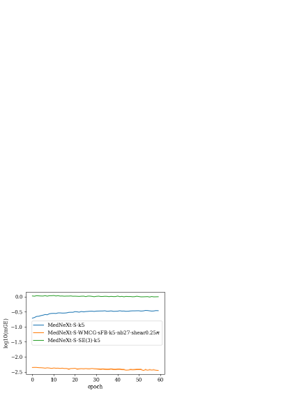
Figure 1: The mGE of the first hidden convolutional layer of the networks.

The results are shown in Table 1. We also report the number of trainable parameters in million ($10^{6}$), Params(M); the number of Multiply–Accumulate Operations in giga ($10^{9}$), MACs(G). We see that a suitable shear angle is beneficial for performance. Large shear angles can harm performance, which may be because large shear angles in discrete implementations can result in a loss of filter information. Random circular shift can slightly boost the performance, which may be because the circular shift can enhance the spatial orthogonality of filters. Anisotropic scaling is shown to reduce the segmentation performance. The possible reason is that the isotropic scaling units (i.e., the pooling method) are more common in deep neural networks. Therefore, in all the following experiments, we adopt isotropic scaling and the default range of shear angles.

It is noted that the kernel reparameterization method proposed in Lee et al. (2023) does not work well with kernel size of $5\times 5\times 5$ and can even reduce the stability of the training.

Table 1: Ablation experimental results on the BTCV dataset.

Models	Params (M)	MAE (G)	DSC
MedNeXt-S-k5-WMCG-sFB-nb27-noshift	5.56	141.94	81.98
MedNeXt-S-k5-WMCG-sFB-nb27-shear0.0	5.56	141.94	81.74
MedNeXt-S-WMCG-sFB-k5-nb27-shear0.25$\pi$	5.56	141.94	82.00
MedNeXt-S-WMCG-sFB-k5-nb27-shear0.40$\pi$	5.56	141.94	81.56
MedNeXt-S-WMCG-sFB-k5-nb27-diffscale	5.56	141.94	81.60
MedNeXt-S-WMCG-sph-k5-nb27-shear0.25$\pi$	5.56	141.94	81.69
MedNeXt-S-k5-REP	5.99	141.94	NaN

3.3 Results with different neural network architectures on abdominal organ segmentation datasets

We test the proposed methods to improve the performance of the state-of-the-art network architectures including nnUNetIsensee et al. (2021) MedNeXtRoy et al. (2023), D-LKA NetAzad et al. (2024), UNETRHatamizadeh et al. (2022), UNETR++Shaker et al. (2022), UXNetLee et al. (2022), and RepUXNetLee et al. (2023).

The experimental results are shown in Table 2 and Table 3. In the names of the tested models, SE(3) means the SE(3) group convolutional layer from Weiler et al. (2018). In the results, "NaN" means that training loss "not a number" error ocurred in the training with both the default learning rate and the ten times smaller learning rate.

MedNeXt-L-k5+SE(3) is constructed by replacing all hidden $5\times 5\times 5$-kernel convolutional layers with the corresponding SE(3)Weiler et al. (2018) G-CNN layers with the same kernel size. MedNeXt-S+WMCG-sFB-k5-nb27 and MedNeXt-L+WMCG-sFB-k5-nb27 are constructed by replacing all hidden $5\times 5\times 5$-kernel convolutional layers with the proposed WMCG-sFB-k5-nb27 G-CNN layers using the first 27 bases. "upkern-retrain" is the kernel upscaling retraining method from Roy et al. (2023), where the $3\times 3\times 3$ kernels from a trained MedNeXt are upscaled to initialize the to-be-trained $5\times 5\times 5$ MedNeXt. "bases_ext" is our proposed method for extending the number of bases in the trained WMCG-sFB layers from 27 to 125 in retraining, where the trained 27 bases are reused.

D-LKA Net+SE(3) is constructed by replacing all the $7\times 7\times 7$ convolutional layers with the corresponding SE(3) layers followed by a $1\times 1\times 1$convolutional layer. D-LKA Net+WMCG-sFB is constructed by replacing all the $7\times 7\times 7$ convolutional layers with the corresponding WMCG-sFB layer followed by a $1\times 1\times 1$convolutional layer.

RepUXNet+SE(3) is constructed by replacing all the hidden $3\times 3\times 3$ layers with the bottleneck block from MedNeXt, where the first convolutional layer is further replaced with a corresponding SE(3) layer but with the number of channel groups as 8. RepUXNet+WMCG-sFB is built by replacing the SE(3) layer in RepUXNet+SE(3) with a corresponding WMCG-sFB layer.

The experimental results in Table 2 and Table 3 show that our methods achieve superior performance to the existing SE(3) G-CNN layers consistently on the two different datasets. Our method is more efficient in training time than the kernel upscaling training method in Roy et al. (2023) and helps improving the performance of the state-of-the-art 3D neural networks.

We also display the mean group-equivariant error (mGE) in Fig. 1 for the first hidden convolutional layers in the training of the first 60 epochs. The mGE is defined as $mGE=\mathbb{E}(\|\phi(\mathbb{T}_{g}(f))-\mathbb{T}^{\prime}_{g}(\phi(f))\|)$. For calculation, for each input image, a randomly generated affine transformation $g\in G$ is used with the shear range $[-0.0625\pi,0.0625\pi)$, the scaling range $[1.0,1.1)$ and rotation angle range $[-0.125\pi,0.125\pi)$. It is shown that our method gives the smallest mGE, which allow the neural network to have a faster convergence from the beginning of the training.

Table 2: Results on the BTCV dataset.

Models	Params (M)	MAE (G)	DSC
nnUNetIsensee et al. (2021)	16.46	186.57	83.00
UNETRHatamizadeh et al. (2022)	92.95	149.08	71.16
UNETR++Shaker et al. (2022)	42.97	77.30	81.06
UXNETLee et al. (2022)	53.01	1159.10	79.38
RepUXNetLee et al. (2023)	65.83	1410.37	NaN
MedNeXt-S-k3Roy et al. (2023)	5.56	109.66	82.89
MedNeXt-S-k5Roy et al. (2023)	5.99	141.94	82.53
MedNeXt-S-k5+SE(3)	5.63	141.94	82.48
MedNeXt-S-k5+WMCG-sFB-nb27	5.56	141.94	83.10
MedNeXt-L-k3Roy et al. (2023)	61.79	419.46	83.44
MedNeXt-L-k5Roy et al. (2023)	63.01	473.73	NaN
MedNeXt-L-k5+SE(3)	61.62	473.73	82.91
MedNeXt-L-k5+WMCG-sFB-nb27	63.01	473.73	83.56
MedNeXt-L-k5+upkern-retrainRoy et al. (2023)	63.01	473.73	83.59
MedNeXt-L-k5+WMCG-sFB-nb125-bases_ext	63.01	473.73	83.61

Table 3: Results on the NIH Pancreas dataset.

Models	Params (M)	MAE (G)	DSC
UNETRHatamizadeh et al. (2022)	92.45	63.53	77.42
UNETR++Shaker et al. (2022)	96.77	102.44	80.59
UXNetLee et al. (2022)	53.01	579.55	83.37
D-LKA NetAzad et al. (2024)	62.07	166.63	81.22
D-LKA Net+SE(3)	61.67	168.04	81.66
D-LKA Net+WMCG-sFB	62.39	168.04	82.42
MedNeXt-L-k3Roy et al. (2023)	61.78	209.44	82.98
MedNeXt-L-k5Roy et al. (2023)	62.99	236.57	82.92
MedNeXt-L-k5-upkern-retrainRoy et al. (2023)	62.99	236.57	83.12
MedNeXt-L-k5+SE(3)	61.62	236.57	80.66
MedNeXt-L-k5+WMCG-sFB	62.99	236.57	83.29
RepUXNetLee et al. (2023)	65.83	704.68	83.75
RepUXNet+SE(3)	47.24	679.04	83.04
RepUXNet+WMCG-sFB	50.51	679.04	84.01

3.4 Discussions

3.4.1 Training stability

From the results on BTCV dataset, we note that the proposed network has superior training stability than plain MedNeXt. This is probably because WMCG-CNN uses bases of low frequency. In addition, the filter decomposition decouples the kernel size and the number of trainable parameters, which allows easier training. SE(3)Weiler et al. (2018); Cesa et al. (2021) also shows good training stability but has inferior segmentation quality. REPLee et al. (2023) can only work on large convolutional kernels and cause instability on middle-level kernel sizes such as $5\times 5\times 5$. Kernel upscalingRoy et al. (2023) can also improve the stability but needs significantly more training time.

3.4.2 Data efficiency

From the experiments on small-scale datasets such as BTCV dataset, we see that the proposed method shows superior data efficiency, which is embodied by its superior DSC results. The data efficiency of the proposed method can be explained by its superior group equivariance layers in training (shown in Fig. 1), as well as its low-frequency filter bases. We note that the SE(3)Weiler et al. (2018); Cesa et al. (2021) approaches give an inferior performance. This is because its filter bases have weaker representation abilities than our methods. Also, its parameter-sharing design limits the number of trainable parameters it can use. In addition, SE(3) only considers rotation and translation equivariance, while in real-world medical data, shear and scaling equivariance are also important. Kernel upscalingRoy et al. (2023) is another method that works well on the small-scale dataset. However, it significantly increases the training time.

3.4.3 Flexibility

It is clear that due to the filter decomposition strategy we use, our methods decouple the number of the trainable parameters and the kernel sizes. It also allows the freedom to select the filter bases or to design particular filter bases. Results on NIH Pancreas datasets show how to use the proposed network layer to improve the performance of the existing state-of-the-art neural network models. For optimal performance, the proposed convolutional layer should be followed by a corresponding convolutional layer. Such structure design has been widely adopted in some existing works such as ResNeXtXie et al. (2017) and ConvNeXtLiu et al. (2022).

4 Conclusion

In this work, we propose an efficient non-parameter-sharing 3D affine G-CNN by weighted aggregation of Monte Carlo augmented spherical Fourier-Bessel bases. The proposed method is superior to the state-of-the-art 3D G-CNN for medical image segmentation. The proposed methods consistently improve the performance of the state-of-the-art 3D segmentation neural networks on small-scale medical image datasets with high training stability and data efficiency. However, it should be noted that the proposed methods are not good at dealing with extremely large kernels such as $21\times 21\times 21$, where an extremely large number of filter bases are needed and can bring a huge memory burden to the GPU machine. How to mitigate this problem will be studied in future work.

Appendix: Proof of Theorem 2.1

Proof.

First, we know that $M(a)$’s determinant $|M(a)|=2^{\alpha+\beta+\gamma}>0$. Thus, all the 3D matrices generated by (13) belongs to $GL^{+}(3,\mathbb{R})$.

Second, considering any 3D matrix $\mathbf{Y}$ with a positive determinant, we need to find a suitable vector $a$ so that $M(a)=\mathbf{Y}$, such decomposition is equivalent to its inverse $M^{-1}(a)=\mathbf{Y}^{-1}$.

According to the properties of shear transform matrices, it is easier to know that by choosing suitable shear values (ie., $s_{01},s_{10},s_{02},s_{20},s_{12},s_{21}$), we can have

$$S_{20}(s_{20})S_{10}(s_{10})S_{21}(s_{21})S_{01}(s_{01})\cdot$$ (26)

$$S_{12}(s_{12})S_{02}(s_{02})\mathbf{Y}^{-1}=\mathbf{D}$$

where

$$\mathbf{D}=\begin{bmatrix}a&0&0\\ 0&b&0\\ 0&0&c\end{bmatrix},$$ (27)

and $abc>0$, $a,b,c\in\mathbb{R}$.

Therefore, for decomposing $Y$ into the form of (13), we only need to further have

$$A_{3}(-\gamma)A_{2}(-\beta)A_{1}(-\alpha)R_{3}(-\theta_{3})R_{1}(-\theta_{1})=\mathbf{D}.$$ (28)

When $a>0$, $b>0$, and $c>0$, we have $\alpha=-\log_{2}(a)$, $\beta=-\log_{2}(b)$, $\gamma=-\log_{2}(c)$, $\theta_{1}=0$, and $\theta_{3}=0$;

When $a>0$, $b<0$, and $c<0$, we have $\alpha=-\log_{2}(a)$, $\beta=-\log_{2}(-b)$, $\gamma=-\log_{2}(-c)$, $\theta_{1}=0$, and $\theta_{3}=\pi$;

When $a<0$, $b<0$, and $c>0$, we have $\alpha=-\log_{2}(-a)$, $\beta=-\log_{2}(-b)$, $\gamma=-\log_{2}(c)$, $\theta_{1}=\pi$, and $\theta_{3}=0$;

When $a<0$, $b>0$, and $c<0$, we have $\alpha=-\log_{2}(-a)$, $\beta=-\log_{2}(b)$, $\gamma=-\log_{2}(-c)$, $\theta_{1}=\pi$, and $\theta_{3}=\pi$.

The proof is complete.

∎

References

- Fukushima [1980] Kunihiko Fukushima. Neocognitron: A self-organizing neural network model for a mechanism of pattern recognition unaffected by shift in position. Biological cybernetics, 36(4):193–202, 1980.
- LeCun et al. [1989] Yann LeCun, Bernhard Boser, John S Denker, Donnie Henderson, Richard E Howard, Wayne Hubbard, and Lawrence D Jackel. Backpropagation applied to handwritten zip code recognition. Neural computation, 1(4):541–551, 1989.
- Isensee et al. [2021] Fabian Isensee, Paul F Jaeger, Simon AA Kohl, Jens Petersen, and Klaus H Maier-Hein. nnu-net: a self-configuring method for deep learning-based biomedical image segmentation. Nature methods, 18(2):203–211, 2021.
- Hatamizadeh et al. [2022] Ali Hatamizadeh, Yucheng Tang, Vishwesh Nath, Dong Yang, Andriy Myronenko, Bennett Landman, Holger R Roth, and Daguang Xu. Unetr: Transformers for 3d medical image segmentation. In Proceedings of the IEEE/CVF winter conference on applications of computer vision, pages 574–584, 2022.
- Roy et al. [2023] Saikat Roy, Gregor Koehler, Constantin Ulrich, Michael Baumgartner, Jens Petersen, Fabian Isensee, Paul F Jaeger, and Klaus H Maier-Hein. Mednext: transformer-driven scaling of convnets for medical image segmentation. In International Conference on Medical Image Computing and Computer-Assisted Intervention, pages 405–415. Springer, 2023.
- Shaker et al. [2022] Abdelrahman Shaker, Muhammad Maaz, Hanoona Rasheed, Salman Khan, Ming-Hsuan Yang, and Fahad Shahbaz Khan. Unetr++: delving into efficient and accurate 3d medical image segmentation. arXiv preprint arXiv:2212.04497, 2022.
- Huang et al. [2023] Tianjin Huang, Lu Yin, Zhenyu Zhang, Li Shen, Meng Fang, Mykola Pechenizkiy, Zhangyang Wang, and Shiwei Liu. Are large kernels better teachers than transformers for convnets? arXiv preprint arXiv:2305.19412, 2023.
- Azad et al. [2024] Reza Azad, Leon Niggemeier, Michael Hüttemann, Amirhossein Kazerouni, Ehsan Khodapanah Aghdam, Yury Velichko, Ulas Bagci, and Dorit Merhof. Beyond self-attention: Deformable large kernel attention for medical image segmentation. In Proceedings of the IEEE/CVF Winter Conference on Applications of Computer Vision, pages 1287–1297, 2024.
- Lee et al. [2023] Ho Hin Lee, Quan Liu, Shunxing Bao, Qi Yang, Xin Yu, Leon Y Cai, Thomas Z Li, Yuankai Huo, Xenofon Koutsoukos, and Bennett A Landman. Scaling up 3d kernels with bayesian frequency re-parameterization for medical image segmentation. In International Conference on Medical Image Computing and Computer-Assisted Intervention, pages 632–641. Springer, 2023.
- Kondor and Trivedi [2018] Risi Kondor and Shubhendu Trivedi. On the generalization of equivariance and convolution in neural networks to the action of compact groups. In International Conference on Machine Learning, pages 2747–2755. PMLR, 2018.
- Qiu et al. [2018] Qiang Qiu, Xiuyuan Cheng, Guillermo Sapiro, et al. Dcfnet: Deep neural network with decomposed convolutional filters. In International Conference on Machine Learning, pages 4198–4207. PMLR, 2018.
- Cohen and Welling [2016a] Taco S Cohen and Max Welling. Steerable cnns. arXiv preprint arXiv:1612.08498, 2016a.
- Lenc and Vedaldi [2015] Karel Lenc and Andrea Vedaldi. Understanding image representations by measuring their equivariance and equivalence. In Proceedings of the IEEE conference on computer vision and pattern recognition, pages 991–999, 2015.
- Wang et al. [2022] Rui Wang, Robin Walters, and Rose Yu. Data augmentation vs. equivariant networks: A theory of generalization on dynamics forecasting. arXiv preprint arXiv:2206.09450, 2022.
- Quiroga et al. [2020] Facundo Quiroga, Franco Ronchetti, Laura Lanzarini, and Aurelio F Bariviera. Revisiting data augmentation for rotational invariance in convolutional neural networks. In Modelling and Simulation in Management Sciences: Proceedings of the International Conference on Modelling and Simulation in Management Sciences (MS-18), pages 127–141. Springer, 2020.
- Cohen and Welling [2016b] Taco Cohen and Max Welling. Group equivariant convolutional networks. In International conference on machine learning, pages 2990–2999. PMLR, 2016b.
- Sangalli et al. [2021] Mateus Sangalli, Samy Blusseau, Santiago Velasco-Forero, and Jesus Angulo. Scale equivariant neural networks with morphological scale-spaces. In Discrete Geometry and Mathematical Morphology: First International Joint Conference, DGMM 2021, Uppsala, Sweden, May 24–27, 2021, Proceedings, pages 483–495. Springer, 2021.
- Sosnovik et al. [2019] Ivan Sosnovik, Michał Szmaja, and Arnold Smeulders. Scale-equivariant steerable networks. arXiv preprint arXiv:1910.11093, 2019.
- Sosnovik et al. [2021] Ivan Sosnovik, Artem Moskalev, and Arnold Smeulders. Disco: accurate discrete scale convolutions. arXiv preprint arXiv:2106.02733, 2021.
- Zhu et al. [2022] Wei Zhu, Qiang Qiu, Robert Calderbank, Guillermo Sapiro, and Xiuyuan Cheng. Scaling-translation-equivariant networks with decomposed convolutional filters. Journal of machine learning research, 23(68):1–45, 2022.
- Gao et al. [2021] Liyao Gao, Guang Lin, and Wei Zhu. Deformation robust roto-scale-translation equivariant cnns. arXiv preprint arXiv:2111.10978, 2021.
- Zhao et al. [2023] Wenzhao Zhao, Barbara D Wichtmann, Steffen Albert, Angelika Maurer, Frank G Zöllner, Ulrike Attenberger, and Jürgen Hesser. Adaptive aggregation of monte carlo augmented decomposed filters for efficient group-equivariant convolutional neural network. arXiv preprint arXiv:2305.10110, 2023.
- Thomas et al. [2018] Nathaniel Thomas, Tess Smidt, Steven Kearnes, Lusann Yang, Li Li, Kai Kohlhoff, and Patrick Riley. Tensor field networks: Rotation-and translation-equivariant neural networks for 3d point clouds. arXiv preprint arXiv:1802.08219, 2018.
- Zhu et al. [2023] Minghan Zhu, Maani Ghaffari, William A Clark, and Huei Peng. E2pn: Efficient se (3)-equivariant point network. In Proceedings of the IEEE/CVF Conference on Computer Vision and Pattern Recognition, pages 1223–1232, 2023.
- Zhdanov et al. [2023] Maksim Zhdanov, Nico Hoffmann, and Gabriele Cesa. Implicit convolutional kernels for steerable cnns. In Thirty-seventh Conference on Neural Information Processing Systems, 2023.
- Shen et al. [2024] Wen Shen, Zhihua Wei, Qihan Ren, Binbin Zhang, Shikun Huang, Jiaqi Fan, and Quanshi Zhang. Rotation-equivariant quaternion neural networks for 3d point cloud processing. IEEE Transactions on Pattern Analysis and Machine Intelligence, 2024.
- Weiler et al. [2018] Maurice Weiler, Mario Geiger, Max Welling, Wouter Boomsma, and Taco S Cohen. 3d steerable cnns: Learning rotationally equivariant features in volumetric data. Advances in Neural Information Processing Systems, 31, 2018.
- Cesa et al. [2021] Gabriele Cesa, Leon Lang, and Maurice Weiler. A program to build e (n)-equivariant steerable cnns. In International Conference on Learning Representations, 2021.
- Xie et al. [2018] Pengtao Xie, Wei Wu, Yichen Zhu, and Eric Xing. Orthogonality-promoting distance metric learning: convex relaxation and theoretical analysis. In International Conference on Machine Learning, pages 5403–5412. PMLR, 2018.
- Binney and Quinn [1991] James Binney and Thomas Quinn. Gaussian random fields in spherical coordinates. Monthly Notices of the Royal Astronomical Society, 249(4):678–683, 1991.
- Fisher et al. [1995] Karl B Fisher, Ofer Lahav, Yehuda Hoffman, Donald Lynden-Bell, and Saleem Zaroubi. Wiener reconstruction of density, velocity and potential fields from all-sky galaxy redshift surveys. Monthly Notices of the Royal Astronomical Society, 272(4):885–908, 1995.
- Landman et al. [2015] Bennett Landman, Zhoubing Xu, J Igelsias, Martin Styner, T Langerak, and Arno Klein. Miccai multi-atlas labeling beyond the cranial vault–workshop and challenge. In Proc. MICCAI Multi-Atlas Labeling Beyond Cranial Vault—Workshop Challenge, volume 5, page 12, 2015.
- Roth et al. [2015] Holger R Roth, Le Lu, Amal Farag, Hoo-Chang Shin, Jiamin Liu, Evrim B Turkbey, and Ronald M Summers. Deeporgan: Multi-level deep convolutional networks for automated pancreas segmentation. In Medical Image Computing and Computer-Assisted Intervention–MICCAI 2015: 18th International Conference, Munich, Germany, October 5-9, 2015, Proceedings, Part I 18, pages 556–564. Springer, 2015.
- Azad [2024] Reza Azad. The nih pancreas dataset, 2024. URL https://github.com/xmindflow/deformableLKA/tree/main/3D.
- Lee et al. [2022] Ho Hin Lee, Shunxing Bao, Yuankai Huo, and Bennett A Landman. 3d ux-net: A large kernel volumetric convnet modernizing hierarchical transformer for medical image segmentation. arXiv preprint arXiv:2209.15076, 2022.
- Xie et al. [2017] Saining Xie, Ross Girshick, Piotr Dollár, Zhuowen Tu, and Kaiming He. Aggregated residual transformations for deep neural networks. In Proceedings of the IEEE conference on computer vision and pattern recognition, pages 1492–1500, 2017.
- Liu et al. [2022] Zhuang Liu, Hanzi Mao, Chao-Yuan Wu, Christoph Feichtenhofer, Trevor Darrell, and Saining Xie. A convnet for the 2020s. In Proceedings of the IEEE/CVF conference on computer vision and pattern recognition, pages 11976–11986, 2022.