Quantum correlations in the steady state of light-emitter ensembles from perturbation theory

Abstract

The coupling of a quantum system to an environment leads generally to decoherence, and it is detrimental to quantum correlations within the system itself. Yet some forms of quantum correlations can be robust to the presence of an environment – or may even be stabilized by it. Predicting (let alone understanding) them remains arduous, given that the steady state of an open quantum system can be very different from an equilibrium thermodynamic state; and its reconstruction requires generically the numerical solution of the Lindblad equation, which is extremely costly for numerics. Here we focus on the highly relevant situation of ensembles of light emitters undergoing spontaneous decay; and we show that, whenever their Hamiltonian is perturbed away from a U(1) symmetric form, steady-state quantum correlations can be reconstructed via pure-state perturbation theory. Our main result is that in systems of light emitters subject to single-emitter or two-emitter driving, the steady state perturbed away from the U(1) limit generically exhibits spin squeezing; and it has minimal uncertainty for the collective-spin components, revealing that squeezing represents the optimal resource for entanglement-assisted metrology using this state.

1 Introduction

Quantum correlations [1], and in particular many-body entanglement [2], are the central resource of quantum many-body devices processing quantum information or simulating complex interacting Hamiltonians [3]. The ability to engineer arbitrary entangled quantum states of e.g a system of $N$ qubits amounts in principle to controlling an exponentially large (in $N$) amount of information – as opposed to linear in $N$ for classical information. Nonetheless quantum information of $N$ qubits is as astronomically large as it is fragile to the presence of an environment. Since information is stored in the relative phases and amplitudes of many-body superposition states, it is extremely sensitive to decoherence and dissipation, generically reducing entangled states to statistical mixtures of states. To counter this effect, the most obvious strategy is to decouple qubits from their environment as much as possible. Yet a more specialized strategy to preserve entanglement in open quantum systems consists in finding forms of entanglement which are robust to the presence of an environment, or that are even stabilized by it. Such robustness to, or assistance from the environment can come from distinct mechanisms. One relevant example is collective dissipation in driven-dissipative systems, in which the degrees of freedom are driven individually, but the elementary dissipation processes can induce entanglement in the system [4]. Through an appropriate engineering of the coupling of the system to the environment, one can obtain steady state entanglement and complex non-equilibrium phases of matter [4, 5, 6, 7]. Another important example is the competition between dissipation (individual or collective) and entangling Hamiltonian dynamics [8, 9, 10, 11]. As a result, the stationary state of the dissipative quantum system can feature entanglement going beyond the paradigm of unitary evolutions, or beyond that of ground-state physics for interacting Hamiltonians.

Understanding the kind of entangled states which can emerge as stationary states of driven-dissipative many-body systems is a formidable theoretical challenge. Indeed reconstructing the stationary state of generic dissipative systems is numerically prohibitive already in systems of $\sim O(10)$ elementary degrees of freedom (such as qubit ensembles). And approximation schemes to tackle the stationary state are often limited in the amount of entanglement that they can describe, either within the system itself (such as in mean-field approaches [9]); or of the system with the environment (such as in approaches based on reduced Hilbert spaces [12]). A significant effort has been devoted in recent years to the development of methods that can accurately describe the properties of open quantum systems [9, 12, 13, 14, 15, 16, 17, 18, 19, 20, 21, 10]. However, the understanding of their correlation properties remains very challenging, and difficult to guess without a dedicated microscopic calculation.

In this work we offer a framework to understand and predict the correlation properties of stationary states of an important class of dissipative quantum systems, i.e. ensembles of quantum emitters coupled to the vacuum of the electromagnetic field [22]. If the Hamiltonian governing the unitary dynamics of the system has rotation (U(1)) symmetry along the quantization axis of the emitters, then the steady state of the system is trivial, and it corresponds to all the emitters in their ground state. We show that a U(1)-symmetry-breaking perturbation in the Hamiltonian, if treated within pure-state perturbation theory, induces quantum correlations in the steady state. This happens at first order in the perturbation, if the perturbation drives pairs of emitters; or at second order, if the perturbation drives individual emitters independently. In particular, the perturbed states possess a very clear form of quantum correlations, i.e. spin squeezing, and they have minimal uncertainty for the collective-spin operators, so that squeezing is their optimal metrological resource [23]. The perturbative calculations can be fully worked out in the case of collective-spin models with individual or collective emission; they allow one to understand the steady state as a perturbed, arbitrarily excited eigenstate of the system’s Hamiltonian; and they can be tested successfully against exact results. The insight gained from these reference models serves as a very useful template for the understanding of more complex situations of models with spatially structured interactions and/or spatially structured collective emission, of direct relevance to current experiments on collective light-matter interactions [24, 25].

Our paper is structured as follows: Sec. 2 discusses the general setting of pure-state perturbation theory for the steady state of the dissipative dynamics; Sec.  3 discusses the models of dissipation of interest to this work; Sec. 4 introduces the collective-spin properties used to characterize quantum correlations; Sec 5 applies the perturbative approach to the case of models with two-emitter driving, formulating the condition under which squeezing is expected in the steady state in the form of a "squeezing theorem" for dissipative steady states; Sec. 6 reconstructs the squeezing properties for the collective XYZ model and transverse-field Ising model with single-emitter dissipation; Sec. 7 discusses instead models with single-emitter drive and collective dissipation, with special focus on the driven Dicke model. A discussion of the experimental implications and conclusions are offered in Secs. 8 and  9.

Figure 1: Sketch of the physical situations of interest to this work: (a) the unperturbed reference is a system of light emitters interacting via a U(1)-symmetric Hamiltonian, and emitting photons in the environment; (b) a Hamiltonian perturbation $\lambda H_{1}$ associated with a two-emitter drive, re-exciting (or de-exciting) the emitters in pairs, can break the U(1) symmetry; (c) a single-emitter (Rabi) drive with strength $\Omega$.

2 Pure-state perturbation theory for the steady state of the Lindblad equation

2.1 General setting

The focus of our work are open quantum systems that interact with a Markovian environment, and can be described by a Lindblad master equation [26]

$$\partial_{t}{\rho}={\cal L}[\rho]=-i\left[{H},{\rho}\right]+\sum_{j}\mathcal{D}\left(\sqrt{\gamma_{j}}\leavevmode\nobreak\ {L}_{j}\right)[\rho],$$ (1)

where ${\cal L}[.]$ denotes the Liouvillian superoperator, ${H}$ is the system’s Hamiltonian, ${\rho}$ the system’s density matrix, and $\mathcal{D}\left(\sqrt{\gamma_{j}}\leavevmode\nobreak\ {L}_{j}\right)$ represents the dissipative process associated with the jump operators $\sqrt{\gamma_{j}}\leavevmode\nobreak\ {L}_{j}$, and it reads

$$\mathcal{D}\left(\sqrt{\gamma_{j}}\leavevmode\nobreak\ {L}_{j}\right)[\rho]=\frac{\gamma_{j}}{2}\left(2{L}_{j}{\rho}{L}_{j}^{\dagger}-\left\{{L}_{j}^{\dagger}{L}_{j},{\rho}\right\}\right).$$ (2)

Our goal is the search of the steady state $\rho_{ss}$ such that ${\cal L}[\rho_{\rm ss}]=0$. The general setting for perturbation theory of Markovian open quantum systems [27, 28, 29, 30, 31, 32] assumes that the Liouvillian can be written as ${\cal L}={\cal L}_{0}+\lambda{\cal L}_{1}$, where ${\cal L}_{0}[.]=-i[H_{0},(.)]+\sum_{j}\mathcal{D}_{0}\left(\sqrt{\gamma_{j}}\leavevmode\nobreak\ {L}_{j}\right)[.]$ is an unperturbed Liouvillian for which the steady state ($\rho_{\rm ss}=\rho_{0}$) is known; while $\lambda{\cal L}_{1}$ is a perturbation, parametrized by $\lambda\in\mathbb{R}$. Since our focus is on elementary mechanisms inducing quantum correlations in the steady state, we shall specialize our interest to the case in which

1. the unperturbed steady state is a unique, pure state, $\rho_{0}=|\phi_{0}\rangle\langle\phi_{0}|$, corresponding to an eigenstate of $H_{0}$, and such that, for all $j$, $L_{j}|\phi_{0}\rangle=0$;

2. the perturbation is purely Hamiltonian, and the perturbed Hamiltonian reads $H=H_{0}+\lambda H_{1}$.

The relevance of the above assumptions to experiments is rather clear. The steady state of systems of $N$ degrees of freedom coupled to a dissipative environment is typically one in which each degree of freedom loses all its energy to the environment, and falls to its single-body ground state, so that $\sum_{j}\mathcal{D}_{0}\left(\sqrt{\gamma_{j}}\leavevmode\nobreak\ {L}_{j}\right)[\rho_{0}]=0$; and at the same time this state is also a (generically excited) eigenstate of the many-body Hamiltonian $H_{0}$, ${H}_{0}|\phi_{0}\rangle=E_{0}|\phi_{0}\rangle$ so that $[H_{0},\rho_{0}]=0$. This is the case e.g. of light emitters (real or artificial atoms) which are not driven, and which therefore decay to their single-body ground state after having emitted. A most natural way of perturbing this steady state in an experiment is to perturb the Hamiltonian with a driving term $\lambda H_{1}$ which alters its symmetry, such that $[H_{0}+\lambda H_{1},\rho_{0}]\neq 0$.

We want to stress that the perturbation $\lambda H_{1}$, although involving the Hamiltonian only, should be still viewed as a perturbation to the Liouvillian super-operator, i.e. as $\lambda{\cal L}_{1}[.]=i\lambda[H_{1},(.)]$. And its smallness should not be measured in comparison with the Hamiltonian term of the Liouvillian only (which may be vanishing, as we will see in the examples offered in this work); but also in comparison with the dissipative part.

The perturbed steady state can be written in general as a power series of the perturbation

$$\rho_{\rm ss}=\rho_{0}+\lambda\rho_{1}+\lambda^{2}\rho_{2}+...$$ (3)

and this state will be generically a mixed state. Yet, since $\rho_{0}$ is pure, we can imagine that the corrections $\lambda\rho_{1}$, $\lambda^{2}\rho_{2}$, etc. alter minimally its purity, so that the perturbed state can in fact be searched for in the form of a pure state as well. Under this assumption we write $\rho_{\rm ss}$ as $|\phi_{0}^{\prime}\rangle\langle\phi_{0}^{\prime}|$ with

$$|\phi_{0}^{\prime}\rangle=|\phi_{0}\rangle+\lambda|\psi_{1}\rangle+\lambda^{2}|\psi_{2}\rangle+...$$ (4)

so that

$$\rho_{ss} \approx\leavevmode\nobreak\ \rho_{0}+\lambda\left(|\phi_{0}\rangle\langle\psi_{1}|+|\psi_{1}\rangle\langle\phi_{0}|\right)$$

$$+\lambda^{2}\left(|\psi_{1}\rangle\langle\psi_{1}|+|\psi_{2}\rangle\langle\phi_{0}|+|\phi_{0}\rangle\langle\psi_{2}|\right)+O(\lambda^{3})\leavevmode\nobreak\ .$$ (5)

Here we shall provide the main results of pure-state perturbation theory relevant for the study provided below.

Injecting the expansion Eq. (3) into the Lindblad equation, imposing the condition of stationarity, and equating terms of same order in $\lambda$, one obtains the following conditions on the first- and second-order corrections to the steady state:

$$\dot{\rho}_{1} =-i[H_{0},\rho_{1}]-i[H_{1},\rho_{0}]$$ (6)

$$+\sum_{j}\gamma_{j}\left[L_{j}\rho_{1}L_{j}^{\dagger}-\frac{1}{2}\{L^{\dagger}_{j}L_{j},\rho_{1}\}\right]=0,$$

$$\dot{\rho}_{2} =-i[H_{0},\rho_{2}]-i[H_{1},\rho_{1}]$$ (7)

$$+\sum_{j}\gamma_{j}\left[L_{j}\rho_{2}L_{j}^{\dagger}-\frac{1}{2}\{L^{\dagger}_{j}L_{j},\rho_{2}\}\right]=0.$$

Given the Hamiltonian eigenbasis $H|\phi_{n}\rangle=E_{n}|\phi_{n}\rangle$, and assuming the unperturbed steady state $|\phi_{0}\rangle$ to be a non-degenerate eigenstate of $H$, we can decompose the pure-state perturbations $|\psi_{1}\rangle$ and $|\psi_{2}\rangle$ in Eq. (4) on the $\{|\phi_{n}\rangle\}$ basis as

$$|\psi_{1}\rangle =\sum_{n\neq 0}c_{n}|\phi_{n}\rangle$$

$$|\psi_{2}\rangle =\left(1-\frac{1}{2}\langle\psi_{1}|\psi_{1}\rangle\right)|\phi_{0}\rangle+\sum_{n\neq 0}d_{n}|\phi_{n}\rangle\leavevmode\nobreak\ .$$ (8)

As in ordinary perturbation theory for Hamiltonian eigenstates [33], the first-order correction can be taken to be orthogonal to the unperturbed state, while the second-order one needs to have overlap with the unperturbed state in order to enforce normalization of the perturbed state.

Imposing the conditions of stationarity, Eqs. (6)-(7), on the states $|\psi_{1}\rangle$ and $|\psi_{2}\rangle$, and projecting them onto the Hamiltonian eigenstates $\langle\phi_{n}|$ from the left and $|\phi_{0}\rangle$ from the right, leads to the following coupled equations for the $c_{n}$ and $d_{n}$ coefficients:

$$(E_{n}-E_{0})c_{n}+\langle\phi_{n}|H_{1}|\phi_{0}\rangle$$ (9)

$$-\frac{i}{2}\sum_{m}c_{m}\langle\phi_{n}|\sum_{j}\gamma_{j}L^{\dagger}_{j}L_{j}|\phi_{m}\rangle=0,\leavevmode\nobreak\$$

$$\left(E_{n}-E_{0}\right)d_{n}+\langle\phi_{n}|H_{1}|\psi_{1}\rangle-c_{n}\langle\phi_{0}|H_{1}|\phi_{0}\rangle$$

$$+i\sum_{j}\gamma_{j}\langle\phi_{n}|L_{j}|\psi_{1}\rangle\langle\psi_{1}|L_{j}^{\dagger}|\phi_{0}\rangle$$

$$-\frac{i}{2}\sum_{j}\sum_{m}\gamma_{j}\langle\phi_{n}|L_{j}^{\dagger}L_{j}|\phi_{m}\rangle d_{m}=0$$ (10)

where in the second equation we have kept the $|\psi_{1}\rangle$ symbol for the sake of brevity.

The above equations clearly provide the formal solution to the perturbation problem if the matrix elements of the Hamiltonian perturbation $H_{1}$ and of the jump operators $L_{j},L_{j}^{\dagger}$ on the basis of the unperturbed Hamiltonian eigenstates are known. We would like to stress that this aspect is made possible because we are restricting our attention to the steady state of the Lindblad dynamics, and we are taking it as a pure state. Previous works [27, 28, 29] have rather tackled the more ambitious problem of reconstructing the full perturbed Liouvillian spectrum and the corresponding generalized eigenvectors. This problem is significantly more involved, as the equations defining the perturbation to the generalized eigenvectors require the pseudo-inversion of non-Hermitian super-operators.

2.2 Special case: $\sum_{j}\gamma_{j}L^{\dagger}_{j}L_{j}$ commutes with the unperturbed Hamiltonian

A special case – relevant to all the examples that we shall provide in the following – is the one in which the jump operators satisfy the following condition

$$[\sum_{j}\gamma_{j}L^{\dagger}_{j}L_{j},H_{0}]=0\leavevmode\nobreak\ .$$ (11)

For this choice of jump operators, $\sum_{j}\gamma_{j}L^{\dagger}_{j}L_{j}$ is diagonal on the eigenbasis of $H_{0}$, simplifying significantly the equations Eqs. (9)-(2.1) above. Indeed this allows for an explicit expression of the first- and second-order corrections to the pure stationary state:

$$|\psi_{1}\rangle=-\sum_{n\neq 0}\frac{\langle\phi_{n}|H_{1}|\phi_{0}\rangle}{\langle H_{0}^{\rm(NH)}\rangle_{n}-E_{0}}\leavevmode\nobreak\ |\phi_{n}\rangle$$ (12)

$$|\psi_{2}\rangle=$$

$$\sum_{n\neq 0,m\neq 0}\frac{\langle\phi_{n}|H_{1}|\phi_{m}\rangle\langle\phi_{m}|H_{1}|\phi_{0}\rangle}{(\langle{H}_{0}^{\rm(NH)}\rangle_{n}-E_{0})(\langle{H}_{0}^{\rm(NH)}\rangle_{m}-E_{0})}\leavevmode\nobreak\ |\phi_{n}\rangle$$

$$-\sum_{n\neq 0}\frac{\langle\phi_{0}|H_{1}|\phi_{0}\rangle\langle\phi_{n}|H_{1}|\phi_{0}\rangle}{(\langle{H}_{0}^{\rm(NH)}\rangle_{n}-E_{0})^{2}}|\phi_{n}\rangle$$

$$-\frac{1}{2}\sum_{n\neq 0}\frac{|\langle\phi_{n}|H_{1}|\phi_{0}\rangle|^{2}}{\left|\langle{H}_{0}^{\rm(NH)}\rangle_{n}-E_{0}\right|^{2}}\leavevmode\nobreak\ |\phi_{0}\rangle\leavevmode\nobreak\$$

$$-i\sum_{j}\gamma_{j}\sum_{n\neq 0}\frac{\langle\phi_{n}|L_{j}|\psi_{1}\rangle\langle\psi_{1}|L_{j}^{\dagger}|\phi_{0}\rangle}{\langle{H}_{0}^{\rm(NH)}\rangle_{n}-E_{0}}\leavevmode\nobreak\ |\phi_{n}\rangle$$ (13)

Here we have introduced the unperturbed, non-Hermitian (NH) Hamiltonian

$${H}_{0}^{\rm(NH)}={H}_{0}-i\sum_{j}\frac{\gamma_{j}}{2}{L}_{j}^{\dagger}{L}_{j},$$ (14)

such that $\langle{H}_{0}^{\rm(NH)}\rangle_{n}=\langle\phi_{n}|{H}_{0}^{\rm(NH)}|\phi_{n}\rangle=E_{n}-i\sum_{j}\frac{\gamma_{j}}{2}\langle{L}_{j}^{\dagger}{L}_{j}\rangle_{n}$ are the complex, unperturbed eigenenergies of the NH Hamiltonian, possessing otherwise the same eigenbasis as $H_{0}$ thanks to the hypothesis Eq. (11).

Comparing with standard non-degenerate perturbation theory [33] it is immediate to verify that the first-order correction Eq. (12) has the same form as that of the first-order perturbation to the eigenstates in closed systems when replacing $H_{0}\to{H}_{0}^{\rm(NH)}$. The same applies as well to the first three lines of Eq. (13), but the fourth line is instead a new term purely introduced by dissipation.

3 Systems of light emitters

3.1 Individual vs. collective spontaneous emission

In the rest of our work we shall specialize our attention to systems of light emitters – such as real or artificial atoms undergoing spontaneous emission – described as dissipative ensembles of two-level systems or qubits, with ground state $|g\rangle$ and excited state $|e\rangle$. They can be described in terms of spin operators ${\bm{S}}_{i}$ $(i=1,....,N)$, with corresponding spin states $|g\rangle=|\downarrow\rangle$ and $|e\rangle=\uparrow\rangle$ along the quantization axis $z$. A useful quantity in the rest of this work will be the collective spin operator ${\bm{J}}=\sum_{i}{\bm{S}}_{i}$. In the following we will assume the unperturbed Hamiltonian $H_{0}(\{\bm{S}_{i}\})$ to be U(1) symmetric, namely conserving the collective spin component $J^{z}$, $[H_{0},J^{z}]=0$, or, equivalently, the number of excited emitters.

The coupling to the environment will be described in terms of spontaneous emission of photons, in the two limits of 1) individual spontaneous emission and 2) collective spontaneous emission:

1. individual emission: in this case the jump operators are single-spin lowering operators $L_{j}\to S_{i}^{-}$, describing emitters which are all coupled to different light modes. If we assume the decay rates to be uniform, $\gamma_{j}=\gamma$, we have that $\sum_{j}\gamma_{j}L_{j}^{\dagger}L_{j}$ reduces to $\gamma\sum_{i}S_{i}^{+}S_{i}^{-}=\gamma(J^{z}+N/2)$, therefore commuting with the unperturbed Hamiltonian;

2. collective emission: in this case the jump operator is unique, $L_{j}\to J^{-}=\sum_{i}S_{i}^{-}$, describing emission of all emitters into the same light mode. In this case $\sum_{j}\gamma_{j}L_{j}^{\dagger}L_{j}=\frac{\Gamma}{N}J^{+}J^{-}=\frac{\Gamma}{N}\left[{\bm{J}}^{2}-(J^{z})^{2}+J^{z}\right]$. This operator commutes with the unperturbed Hamiltonian when the latter conserves not only the total magnetization, but also the collective spin length, namely if $[{\bm{J}}^{2},H_{0}]=0$.

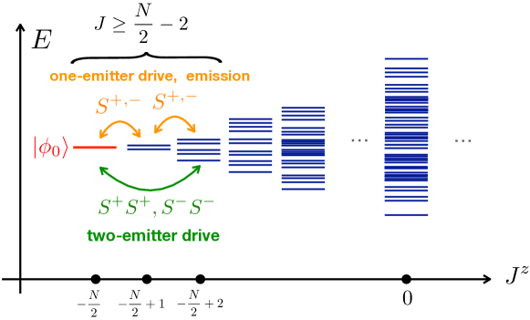
Figure 2: Sketch of perturbation theory from the unperturbed $|\phi_{0}\rangle=|\downarrow\downarrow...\downarrow\rangle$ state. We picture here a generic spectrum of a $U(1)$-symmetric Hamiltonian, whose eigenstates can be labeled by the quantum number $J^{z}$. The two-emitter drive to first order, or the one-emitter drive to second order, connect the unperturbed state, with $J^{z}=-N/2$ and maximum spin length ${\bm{J}}^{2}=J(J+1)$ and $J=N/2$, with states with $J^{z}=-N/2+2$ and spin length $J\geq N/2-2$. Hence the perturbed state is a superposition of highly atypical, large-spin Hamiltonian eigenstates.

For both of the above cases of interest to this work, the pure state $|\phi_{0}\rangle=|gg...g\rangle=|\downarrow\downarrow...\downarrow\rangle$ is the unique steady state of the unperturbed dissipative dynamics. Moreover both cases satisfy the assumption of the previous Sec. 2.2 (adding the extra condition $[{\bm{J}}^{2},H_{0}]=0$ in case 2), which leads to the explicit expressions for the state perturbation as in Eqs. (12)-(13). This situation lends itself to a rather interesting interpretation: the perturbed, pure steady state of the dissipative evolution can be viewed as the perturbed version of the Hamiltonian eigenstate $|\phi_{0}\rangle$ induced by the Hamiltonian $H_{1}$ to first order, and by the $H_{1}$ and the jump operators $L_{j},L_{j}^{\dagger}$ to second order, namely as the perturbation of a (generically) excited Hamiltonian eigenstate. The perturbation operators $H_{1}$ and $L_{j},L_{j}^{\dagger}$ will mainly admix $|\phi_{0}\rangle$ with other excited states in the same energy range, but with a fundamental restriction as we will highlight below.

3.2 Extremal properties of the unperturbed and perturbed state

A relevant $H_{1}$ perturbation to $U(1)$ symmetric Hamiltonians breaks the U(1) symmetry, namely the conservation of the number of excited emitters. This implies that the perturbation corresponds generically to driving, which we will consider as having two different forms (see sketch in Fig. 1): 1) two-emitter drive exciting/de-exciting pairs of emitters together, of the kind $S_{i}^{+}S_{j}^{+}+S_{i}^{-}S_{j}^{-}$ (for $i\neq j$) where $S_{i}^{\pm}=S_{i}^{x}\pm iS_{i}^{y}$ are raising/lowering spin operators; and 2) single-emitter drive, of the kind $S^{+}_{i}+S^{-}_{i}$. The two-emitter drive will be discussed in Secs. 5, while the single-emitter drive will be discussed in Sec. 7.

At this point, it is crucial to understand the special role played by the unperturbed state $|\phi_{0}\rangle$ within perturbation theory. Indeed this state is extremal in that it maximizes (in absolute value) the projection $J^{z}$, and hence the collective spin length ${\bm{J}}^{2}=J(J+1)$ with $J=N/2$. All the operators associated to single-emitter and two-emitter drives, as well as the jump operators $L,L^{\dagger}$ related to emission, can only connect the $|\phi_{0}\rangle$ state to states with $J=N/2-2$ (to first order in the two-emitter drive operators, and to second order in the single-emitter drive and jump operators) – see sketch in Fig. 2. This implies that, to lowest order in perturbation theory, the perturbed state has only support on high-spin Hamiltonian eigenstates, representing a highly atypical portion of the spectrum, even when the unperturbed Hamiltonian $H_{0}$ is chaotic. This aspect suggests that, regardless of the details of the Hamiltonian, the nature of the perturbed steady state will be close to that obtained for models with long-range interactions (both in $H_{0}$ as well as in $H_{1}$), whose eigenstates possess a well defined total spin length ${\bm{J}}^{2}$ with small or no fluctuations. In the rest of this work we will work with collective-spin Hamiltonians, whose choice is not only convenient technically (see below), but also justified by the above remarks.

4 Collective-spin properties and spin squeezing

Before we apply pure-state perturbation theory to specific examples, it is important to introduce the quantities that we shall use to characterize the quantum correlations induced by the perturbation in the steady state of the system.

The unperturbed steady state of our interest $|\phi_{0}\rangle=|\downarrow\downarrow...\downarrow\rangle$ is an example of a coherent spin state (CSS). The collective spin of this state points along the $z$ axis, $\langle J^{z}\rangle=-\frac{N}{2}$, and the transverse spin components have equal uncertainties

$${\rm Var}(J^{x})={\rm Var}(J^{y})=N/4\leavevmode\nobreak\ .$$ (15)

In fact we can extend the above property by considering a generalized definition of the collective spin as having transverse, perpendicular components $J_{1}^{\perp}$ and $J_{2}^{\perp}$, such that $[J_{1}^{\perp},J_{2}^{\perp}]=iJ^{z}$, in the form

$$J_{1}^{\perp}= \sum_{i}\left(\cos\theta_{i}S_{i}^{x}+\sin\theta_{i}S_{i}^{y}\right)$$

$$= \frac{1}{2}\sum_{i}\left(S_{i}^{+}e^{-i\theta_{i}}+S_{i}^{-}e^{i\theta_{i}}\right)\leavevmode\nobreak\ ,$$ (16)

and

$$J_{2}^{\perp}= \sum_{i}\left(-\sin\theta_{i}S_{i}^{x}+\cos\theta_{i}S_{i}^{y}\right)$$

$$= -\frac{1}{2}\sum_{i}\left(S_{i}^{+}e^{i\theta_{i}}+S_{i}^{-}e^{-i\theta_{i}}\right)\leavevmode\nobreak\ .$$ (17)

where $\theta_{i}$ are local angles. For a CSS we have that ${\rm Var}(J_{1}^{\perp})={\rm Var}(J_{2}^{\perp})=N/4$, and in particular ${\rm Var}(J_{1}^{\perp}){\rm Var}(J_{2}^{\perp})=|\langle J^{z}\rangle|^{2}/4$, saturating the Heisenberg uncertainty relation for spin operators. As a consequence the CSS represents an example of a minimal uncertainty state.

As we shall see, Hamiltonian perturbations breaking its U(1) symmetry have the immediate effect of redistributing the uncertainties on the transverse components in the steady state, inducing squeezing of the collective spin. Squeezing of a transverse collective spin component can be quantified by the squeezing parameter [34]

$$\xi^{2}_{R}=\frac{N\min_{\perp}{\rm Var}(J^{\perp})}{\langle J^{z}\rangle^{2}}\leavevmode\nobreak\ .$$ (18)

where the minimization $\min_{\perp}$ is made over all possible choices of the local angles $\theta_{i}$. If $\xi_{R}^{2}<1$ the collective spin exhibits squeezing, which is a fundamental form of quantum correlation. Indeed squeezed states are entangled [35]; and their entanglement has an immediate metrological significance, making them more sensitive to rotations more than any coherent spin state [34].

Because the collective spin components must satisfy the Heisenberg uncertainty relation ${\rm Var}(J_{1}^{\perp}){\rm Var}(J_{2}^{\perp})\geq|\langle J^{z}\rangle|^{2}/4$, if one component (e.g. $J_{1}^{\perp}$) acquires the minimum variance $\min_{\perp}{\rm Var}(J^{\perp})$ and is squeezed (namely $\xi_{R}^{2}<1$), the other one (e.g. $J_{2}^{\perp}$) must be anti-squeezed (namely $\xi_{R}^{2}>1$ for it), and in particular it has the property of exhibiting the largest variance among all the collective-spin components transverse to the average orientation. The anti-squeezed component captures therefore the strongest form of spin-spin correlations appearing in the system. To quantify the quantum nature of these correlations, one can introduce the quantum Fisher information (QFI) associated with $J_{2}^{\perp}$, which is most generally defined for a state $\rho=\sum_{k}p_{k}|k\rangle\langle k|$ (with $|k\rangle$ forming an orthonormal basis) as [36]

$${\rm QFI}(J_{2}^{\perp})=2\sum_{kl}\frac{(p_{k}-p_{l})^{2}}{p_{k}-p_{l}}|\langle k|J_{2}^{\perp}|l\rangle|^{2}\leavevmode\nobreak\ .$$ (19)

In particular the QFI bounds the uncertainty with which one can estimate the angle $\phi$ of a rotation $e^{-i\phi J^{\perp}_{2}}$, generated by the operator $J_{2}^{\perp}$, by making arbitrary measurements on the state, $(\delta\phi)^{2}\geq 1/{\rm QFI}(J_{2}^{\perp})$. The QFI satisfies the inequality (descending from the above bound and the fact that ${\rm QFI}(J_{2}^{\perp})\leq 4{\rm Var}(J_{2}^{\perp})$ [23]):

$$4{\rm Var}(J_{1}^{\perp}){\rm Var}(J_{2}^{\perp})\geq{\rm Var}(J_{1}^{\perp}){\rm QFI}(J_{2}^{\perp})\geq|\langle J^{z}\rangle|^{2}$$ (20)

implying that

$$\xi_{R}^{-2}\leq{\rm QFI}(J_{2}^{\perp})/N\leavevmode\nobreak\ .$$ (21)

If the squeezed state is a state of minimal uncertainty, this means that the inequality chain Eq. (20) collapses to an equality, and in particular that $\xi_{R}^{-2}={\rm QFI}(J_{2}^{\perp})/N$. For such a state squeezing is the optimal metrological resource, namely rotations can be best estimated by simply measuring the average orientation of the collective-spin operator.

5 Two-emitter driving and individual emission: squeezing theorem

5.1 Two-emitter driving

The first example of perturbation that we shall consider is a most general, parity-conserving bilinear Hamiltonian perturbation $H_{1}$ in the form $H_{1}=H_{1,d}+H_{1,o}$ where

$$H_{1,d}=\sum_{lm}\left(J_{lm}S_{l}^{+}S_{m}^{-}+{\rm h.c.}\right)+H_{\rm diag}$$ (22)

is a $J^{z}$-conserving term, and

$$H_{1,o}=\sum_{lm}\left(K_{lm}S_{l}^{+}S_{m}^{+}+{\rm h.c.}\right)\leavevmode\nobreak\$$ (23)

is a $J^{z}$-non-conserving one. Here $H_{\rm diag}$ is an arbitrary Hamiltonian which is diagonal on the eigenbasis of the $S_{i}^{z}$ operators. The perturbation $H_{1,o}$ contains two-emitter driving terms, which are essential to perturb the steady state.

Indeed, given that $[H_{0},J^{z}]=0$, the Hamiltonian eigenstates $|\phi_{n}\rangle$ can be chosen to be also eigenstates of $J^{z}$. In particular $|\phi_{0}\rangle$ is the only state in the $J^{z}=-N/2$ sector. Given that $H_{1,d}$ cannot couple different $J^{z}$ sectors, we have that

$$\langle\phi_{n}|H_{1,d}|\phi_{0}\rangle\sim\delta_{n0}\leavevmode\nobreak\ .$$ (24)

Hence the state $|\phi_{0}\rangle$ can only be perturbed by the $H_{1,o}$ operator. Within that operator the terms of the kind $S_{l}^{+}S_{m}^{+}$ are the only ones that do not annihilate the $|\phi_{0}\rangle$ state, and they map that state onto states belonging to the $J^{z}=-N/2+2$ sector, that we will denote as ${\cal S}_{-N/2+2}$ in the following.

Since the perturbation $H_{1}$ introduces emitter-emitter couplings, it can by itself give rise to quantum correlations in the steady state. Hence we will consider the case of individual (i.e. uncorrelated) spontaneous emission $L_{j}\to S_{i}^{-}$ with a uniform rate $\gamma$ for all emitters. This coupling to the environment has clearly the tendency to decorrelate the emitters. The form of quantum correlations stabilized in the steady state will therefore be of a kind which is robust to a decorrelating environment.

5.2 Squeezing theorem

Applying the formulas of Sec. 2.2, the first-order perturbation to the steady state takes the form

$$|\psi_{1}\rangle=\sum_{n\in{\cal S}_{-N/2+2}}\frac{\langle\phi_{n}|\sum_{lm}K_{lm}S_{l}^{+}S_{m}^{+}|\phi_{0}\rangle}{E_{0}-E_{n}+i\gamma}|\phi_{n}\rangle,$$ (25)

since

$$\frac{1}{2}\langle\phi_{n}|\sum_{i}S_{i}^{+}S_{i}^{-}|\phi_{n}\rangle=\frac{1}{2}(-N/2+2+N/2)=1\leavevmode\nobreak\ .$$ (26)

As a consequence

$$\langle(J^{\perp})^{2}\rangle^{\prime}=\frac{N}{4}+\lambda\left(\langle\phi_{0}|(J^{\perp})^{2}|\psi_{1}\rangle+{\rm c.c.}\right)+O(\lambda^{2}),$$ (27)

where we introduced the short-hand notation for the expectation values on the perturbed state $\langle(...)\rangle^{\prime}=\langle\phi_{0}^{\prime}|(...)|\phi_{0}^{\prime}\rangle$. The matrix element $\langle\phi_{0}|(J^{\perp})^{2}|\psi_{1}\rangle$ can be written as

$$\langle\phi_{0}|(J^{\perp})^{2}|\psi_{1}\rangle=-\frac{1}{4}\sum_{n\in{\cal S}_{-N/2+2}}\frac{\sum_{lm}\sum_{ij}e^{i(\theta_{i}+\theta_{j})}\langle\phi_{n}|K_{lm}S_{l}^{+}S_{m}^{+}|\phi_{0}\rangle\langle\phi_{0}|S_{i}^{-}S_{j}^{-}|\phi_{n}\rangle}{E_{n}-E_{0}-i\gamma}=-F(\{\theta_{i}\})\leavevmode\nobreak\ .$$ (28)

Given that

$$\langle J^{z}\rangle^{\prime}=-\frac{N}{2}+O(\lambda^{2}),$$ (29)

the squeezing parameter to first order takes the value

$$\xi_{R}^{2}=1-\frac{8\lambda}{N}\leavevmode\nobreak\ {\rm Re}[F(\{\theta_{i}\})]+O(\lambda^{2})\leavevmode\nobreak\ .$$ (30)

The above results implies the following

Theorem 1

The steady state of an ensemble of emitters with U(1)-symmetric unperturbed Hamiltonian subject to individual emission – whose unique steady state is $|\phi_{0}\rangle=|\downarrow\downarrow...\rangle$ – is perturbed to a spin-squeezed state (within first-order perturbation theory) by a perturbation of the form of Eq. (23) iff

$$\max_{\{\theta_{i}\}}{\rm Re}[F(\{\theta_{i}\})]>0\leavevmode\nobreak\$$ (31)

where the function $F$ is defined in Eq. (28).

The angles $\{\theta_{i}\}$ maximizing the function ${\rm Re}[F]$ define the generalized collective-spin component $J^{\perp}_{1}$ which is maximally squeezed; and, in turn, the angles $\{\theta_{i}+\pi/2\}$ define the anti-squeezed component $J_{2}^{\perp}$, namely the local spin components $-\sin(\theta_{i})S_{i}^{x}+\cos(\theta_{i})S_{i}^{y}$ which are most strongly correlated with one another between different sites.

If the condition Eq. (31), defining the squeezed transverse component $J^{\perp}_{1}$, is satisfied, then the perpendicular component $J^{\perp}_{2}$ is automatically anti-squeezed since $\langle\phi_{0}|(J_{1}^{\perp})^{2}|\psi_{1}\rangle=-\langle\phi_{0}|(J_{2}^{\perp})^{2}|\psi_{1}\rangle$, and therefore

$$\langle(J^{\perp}_{2})^{2}\rangle^{\prime}=\frac{N}{4}+2\lambda\max_{\{\theta_{i}\}}{\rm Re}[F({\theta_{i}}]+O(\lambda^{2}).$$ (32)

As a consequence, the perturbed state has the property

$$\langle(J^{\perp}_{1})^{2}\rangle^{\prime}\langle(J^{\perp}_{2})^{2}\rangle^{\prime}=\frac{N^{2}}{16}+O(\lambda^{2})=\frac{|\langle J^{z}\rangle^{\prime}|^{2}}{4}+O(\lambda^{2})$$ (33)

namely it is a minimal uncertainty state, for which squeezing is the optimal metrological property.

The above theorem extends to dissipative steady states a simple theorem recently put forward by one of the authors for Hamiltonian ground states [37]. The present result highlights the importance of spin squeezing as the first form of quantum correlation that can be stabilized when perturbing the factorized stead state $|\phi_{0}\rangle$ with a bilinear perturbation (a two-emitter drive). The assumption of having a bilinear perturbation in the spin operators is not a fundamental limitation. If we had included in $H_{1}$ an off-diagonal perturbation which is linear in the spin operators, e.g. proportional to $J^{x}$ or $J^{y}$, this would not change the above results within first-order perturbation theory. Indeed, due to the structure of the squeezing parameter Eq. (18), linear operators in the spins cannot give contributions to first order, because they cannot compensate the effect of the bilinear operator $(J^{\perp})^{2}$ on the unperturbed state (see Eq. (12)). On the other hand they can perturb the state to second order, as we will discuss in Sec. 7.

In the following section we will test the predictions of pure-state perturbation theory and the relevance of spin squeezing in two examples widely studied in the recent literature on dissipative quantum spin models.

6 Application to collective spin Hamiltonians

In the following we will consider collective-spin Hamiltonians of the form

$${H}=\sum_{\alpha=x,y,z}\left[\frac{\mathcal{J}_{\alpha}}{N}(J^{\alpha})^{2}+h_{\alpha}J^{\alpha}\right],$$ (34)

which can be decomposed into an unperturbed, U(1)-symmetric part, and a symmetry-breaking perturbation. Specifically, we will discuss the collective XYZ model [38] and the collective transverse-field Ising model [11] with dissipation in the form of individual emission with uniform decay rates. These models are particularly suitable for a test of our perturbative results, since they admit an efficient numerical solution thanks to the permutational symmetry of their Hamiltonians [15], offering a valuable benchmark. For these numerical simulations we resort to the implementation of the permutational invariant solver in QuTiP [39, 40].

6.1 Example I: the dissipative XYZ model

We consider the collective (or infinite-dimensional) XYZ Heisenberg model [38] with individual spontaneous emission, whose Hamiltonian can be written as

$$H=\frac{1}{N}\sum_{i,j}\left({\cal J}_{x}S_{i}^{x}S_{j}^{x}+{\cal J}_{y}S_{i}^{y}S_{j}^{y}+{\cal J}_{z}S_{i}^{z}S_{j}^{z}\right),$$ (35)

where the sums $\sum_{i(j)}$ run over the $N$ emitters. This Hamiltonian – both in its collective-spin form, as well as when cast on finite-dimensional lattices – has been the subject of many theoretical studies in the recent past [8, 9, 41, 42, 43, 38, 10].

Choosing $\mathcal{J}_{x}=\mathcal{J}_{y}$, one recovers a U(1)-symmetric XXZ model, conserving the magnetization $J^{z}$. The dissipative XXZ model clearly admits the state $|\phi_{0}\rangle=|\downarrow\downarrow...\downarrow\rangle$ as its unique steady state. It is useful to recast the latter state as a Dicke state $|\phi_{0}\rangle=|J=N/2,M=-N/2\rangle$ with maximal spin length ${\bm{J}}^{2}=J(J+1)=N/2(N/2+1)$ and $J^{z}=M$.

The Hamiltonian Eq. (35) can be rewritten in the form

$${H}=H_{0}+\lambda H_{1},$$ (36)

with

$$H_{0}=\frac{\mathcal{J}}{N}\left[(J^{x})^{2}+(J^{y})^{2}\right]+\frac{\mathcal{J}_{z}}{N}(J^{z})^{2},$$ (37)

and

$$\lambda H_{1}=\frac{\delta{\cal J}}{2N}\left[(J^{+})^{2}+(J^{-})^{2}\right]$$ (38)

where we have introduced the symbols

$${\cal J}=\frac{{\cal J}_{x}+{\cal J}_{y}}{2}\leavevmode\nobreak\ \leavevmode\nobreak\ \leavevmode\nobreak\ \leavevmode\nobreak\ \leavevmode\nobreak\ \leavevmode\nobreak\ {\delta\cal J}=\frac{{\cal J}_{x}-{\cal J}_{y}}{2}\leavevmode\nobreak\ .$$ (39)

Given the permutation invariance of the Hamiltonian (including the perturbation), we can choose uniform angles $\theta_{i}=\theta$ in the definition of the transverse spin components Eqs. (16) and (17) without loss of generality. In particular the permutationally invariant perturbation will couple the Dicke state $|\phi_{0}\rangle=|J=N/2,M=-N/2\rangle$ to another Dicke state only, namely $|\phi_{2}\rangle=|J=N/2,M=-N/2+2\rangle$ via a double spin flip. This means that the sum of Eq. (28) collapses to only one state. Moreover Dicke states are all eigenstates of the all-to-all XXZ Hamiltonian with eigenvalues

$$E(J,M)= \langle J,M|H_{0}|J,M\rangle,$$ (40)

$$= \frac{\cal J}{N}J(J+1)+\frac{1}{N}({\cal J}_{z}-{\cal J})M^{2},$$ (41)

so that the only relevant transition energy is $E_{2}-E_{0}=2\left({\cal J}-{\cal J}_{z}\right)\left(N-2\right)/N$.

Moreover we get

$$\langle\phi_{2}|H_{1}|\phi_{0}\rangle =\frac{\delta\cal J}{2N}\left\langle\phi_{2}\right|(J^{+})^{2}\left|\phi_{0}\right\rangle,$$ (42)

$$=\frac{\delta\cal J}{2}\sqrt{2\left(N-1\right)/N}.$$

As a consequence the function $F\left(\{\theta\}\right)$ from theorem 1 takes the form

$$F(\{\theta\})= \frac{1}{8}\frac{\delta{\cal J}(N-1)e^{i2\theta}}{\left({\cal J}-{\cal J}_{z}\right)\left(N-2\right)/N-i\gamma},$$ (43)

$$= \frac{\alpha e^{i2\theta}}{\beta-i\gamma}.$$ (44)

where we introduced the symbols

$$\alpha =\frac{N-1}{4}\leavevmode\nobreak\ \delta{\cal J}$$ (45)

$$\beta =\frac{2(N-2)}{N}\left({\cal J}-{\cal J}_{z}\right)\leavevmode\nobreak\ .$$ (46)

In terms of these symbols the real part of $F$ reads

$${\rm Re}[F(\{\theta\})]=\frac{\alpha\left(\beta\cos 2\theta-\gamma\sin 2\theta\right)}{\beta^{2}+\gamma^{2}}.$$ (47)

Figure 3: (a) Minimal spin squeezing parameter $\xi_{\rm R}^{2}$ as a function of $\delta\mathcal{J}$ for the exact solution (full black lines) and the perturbative solution (dashed colored lines). This corresponds to a perturbation perpendicular to the $\mathcal{J}$ axis (see also Fig. 5). Parameters used are $N=20$, $\mathcal{J}_{z}=\gamma$ , and $\mathcal{J}=-1.8\gamma,-0.8\gamma,-0.2\gamma$ (resp. blue, dark red, and orange, as indicated on the figure). (b) The angle $\phi_{min}$ for which the spin squeezing parameter is minimal (see panel (a)). Same parameters as panel (a) (from top to bottom; $\mathcal{J}=-0.2\gamma,-0.8\gamma,-1.8\gamma$).

6.1.1 Onset of squeezing in the perturbed state

The presence of squeezing in the steady state is then governed by condition (31), and depends on the angle $\theta$. The angle $\theta$ extremizing ${\rm Re}[F(\{\theta_{i}\})]$ is given by (see appendix A)

$$\theta_{ex.}=\frac{1}{2}\tan^{-1}\left(-\frac{\gamma}{\beta}\right)+k\frac{\pi}{2}\quad k\in\mathbb{Z}$$ (48)

and it exhibits a subtle dependence on both the Hamiltonian parameters and the dissipation strength that we will discuss in Sec. 6.1.2.

For the extremal angle $\theta_{\rm ex}$ the real part of the $F$ function takes the form (see appendix A)

$${\rm Re}\left[F(\left\{\theta_{\rm ex}\right\})\right]=\frac{\alpha\cos(k\pi)}{\sqrt{\beta^{2}+\gamma^{2}}}.$$ (49)

The sign of this function (determining the existence of squeezing) depends on the integer $k$ and on the sign of $\alpha$, but it does not depend on the sign of $\beta$. Yet, whenever the perturbation breaks the U(1) symmetry, namely $\alpha\neq 0$, one can always find an extremizing angle for which ${\rm Re}(F)>0$: this is achieved by choosing $k$ even (odd) for $\alpha>0$ ($\alpha<0$). This implies that the U(1)-symmetry-breaking perturbation always induces squeezing in the steady state, as per the above theorem. The above result is clearly exhibited in Fig. 3, where we compare the squeezing parameter predicted by perturbation theory with the exact result for $N=20$ spins as an example. There we see that, as predicted by pure-state perturbation theory, the squeezing parameter $\xi_{R}^{2}$ decreases linearly from its unperturbed unit value. The deviation from the perturbative predictions can clearly be attributed to beyond-linear effects, as well as to the fact that the steady-state develops some finite entropy (albeit subextensive [44]), not accounted for by pure-state perturbation theory.

The prediction of perturbation theory for the squeezing parameter agrees with the exact result over a larger interval of perturbation values when $\mathcal{J}\ll\mathcal{J}_{z}$ and $\mathcal{J}\gg\mathcal{J}_{z}$, namely far away from the SU(2)-symmetric point (for the Hamiltonian) ${\cal J}_{x}={\cal J}_{y}={\cal J}_{z}$. To understand this result it is important to remind that, for a critical value of the perturbation $\delta{\cal J}$ (dependent on the value of ${\cal J}/\gamma$), the steady-state phase diagram features a phase transition [38] from a paramagnetic phase – continuously connected with the unperturbed U(1)-symmetric steady state; to a ferromagnetic phase, which develops long-range correlations for one spin component in the $xy$ plane (see the sketch in Fig. 5, and Sec. 6.1.2 for further discussion). The critical value of $\delta{\cal J}$ is minimal (in absolute value) for ${\cal J}={\cal J}_{z}$ and it grows upon increasing the difference between ${\cal J}$ and ${\cal J}_{z}$. The predictions of perturbation theory break down upon approaching the phase transition, and this occurs for larger $\delta{\cal J}$ values the larger the anisotropy between ${\cal J}$ and ${\cal J}_{z}$. Nonetheless, even when perturbing the steady state away from the SU(2) symmetric point, perturbation theory correctly captures the onset of squeezing, showing that this is a universal feature of the paramagnetic phase close to the U(1)-symmetric line ${\cal J}_{x}={\cal J}_{y}$. As we will discuss in the next section, pure-state perturbation theory also predicts correctly which collective-spin component is squeezed and which one is anti-squeezed; and in this sense, it provides insight into important features of the steady-state phase diagram, even going beyond its strict range of applicability.

Figure 4: Optimal angle $\theta$ in the $(x,y)$-plain that minimises the spin squeezing parameter in the XYZ model as predicted by (a) the perturbative approach and (b) the exact solution for a system with $N=20$ spins and $\mathcal{J}_{z}=\gamma$. Black dashed lines show the mean-field phase transition between the paramagnetic phase and ferromagnetic phase – corresponding to the exact solution for the all-to-all connected model in the thermodynamic limit [38, 45].

6.1.2 Angle of squeezing vs. anti-squeezing; insight into the ferromagnetic phases

Eq. (48) from perturbation theory gives an explicit prediction of the extremal angle for squeezing and anti-squeezing as a function of the Hamiltonian parameter and the dissipation strength. The extremal squeezing angle $\theta_{\rm ex}$ is plotted in Fig. 4 across the steady-state phase diagram, as a function of the ratios ${\cal J}_{x}/\gamma$ and ${\cal J}_{y}/\gamma$ at fixed ${\cal J}_{z}/\gamma=1$, comparing pure-state perturbation theory with the exact result from Ref. [38]. We observe that the subtle dependence of the angle on both the Hamiltonian parameters and the dissipation strength is correctly captured by perturbation theory within its strict regime of applicability, namely within the paramagnetic phase continuously connected with the unperturbed limit ${\cal J}_{x}={\cal J}_{y}$.

In order to make sense of the angle map of Fig. 4, it is instructive to take the limite of a negligible dissipation, i.e. to consider $|\mathcal{J-J}_{z}|\gg\gamma$. In this limit the ratio $\gamma/\beta$ becomes negligible, and therefore one obtains ${\rm Re}[F(\theta)]\approx\alpha\cos(2\theta)/\beta$, which for $\alpha/\beta>0$ is maximized by $\theta=0\leavevmode\nobreak\ ({\rm mod}\leavevmode\nobreak\ \pi)$ and for $\alpha/\beta<0$ it is maximized by $\theta=\pi/2\leavevmode\nobreak\ ({\rm mod}\leavevmode\nobreak\ \pi)$. The two conditions, $\alpha/\beta>0$ and $\alpha/\beta<0$, divide the $({\cal J}_{x},{\cal J}_{y})$ plane into four quadrants, which are oriented with the $\pi/4$-rotated axes $\delta{\cal J}$ and ${\cal J}-{\cal J}_{z}$. The condition $\alpha/\beta>0$ is met when $\delta{\cal J}>0$ and ${\cal J}>{\cal J}_{z}$, defining the quadrant I; or $\delta{\cal J}<0$ and ${\cal J}<{\cal J}_{z}$, defining the quadrant III. In these two quadrants the maximum squeezing angle is therefore $\theta=0\leavevmode\nobreak\ ({\rm mod}\leavevmode\nobreak\ \pi)$. The angle $\theta=\pi/2\leavevmode\nobreak\ ({\rm mod}\leavevmode\nobreak\ \pi)$ is instead the maximum squeezing angle in the quadrant II: $\delta{\cal J}>0$ and ${\cal J}<{\cal J}_{z}$; and quadrant IV: $\delta{\cal J}<0$ and ${\cal J}>{\cal J}_{z}$. The four quadrants with $\theta=0\leavevmode\nobreak\ ({\rm mod}\leavevmode\nobreak\ \pi)$ and $\theta=\pi/2\leavevmode\nobreak\ ({\rm mod}\leavevmode\nobreak\ \pi)$ are clearly visible in Fig. 4(a); and they are repeated in Fig. 5 for clarity. Introducing a finite dissipation $\gamma$ has then the main effect of rounding off the transition between the two values of $\theta=0\leavevmode\nobreak\ ({\rm mod}\leavevmode\nobreak\ \pi)$ or $\pi/2\leavevmode\nobreak\ ({\rm mod}\leavevmode\nobreak\ \pi)$ when moving above or below the ${\cal J}_{x}={\cal J}_{y}$ line.

The angle $\theta$ shown in the figure determines the maximally squeezed component of the collective spin, but correspondingly the angle $\theta+\pi/2\leavevmode\nobreak\ ({\rm mod}\leavevmode\nobreak\ \pi)$ determines the anti-squeezed spin component, developing the strongest ferromagnetic correlations. These correlations become long-ranged across the paramagnetic-to-ferromagnetic transition, whose description is clearly beyond the scopes of perturbation theory. Yet the nature of the ferromagnetic correlations can be understood to a large extent from perturbation theory.

First of all, it is remarkable to see that the dominant correlations are in the $xy$ plane, and they are ferromagnetic regardless of the signs of the Hamiltonian couplings ${\cal J}_{x}$ and ${\cal J}_{y}$. Moreover the spin component exhibiting the strongest correlations does not correspond necessarily to the spin component with the largest Hamiltonian coupling. Perturbation theory predicts that the strongest ferromagnetic correlations are exhibited by the $x$ spin components in quadrants I and III, and by the $y$ spin component in quadrants II and IV; while the strongest coupling in the Hamiltonian is ${\cal J}_{x}$ in quadrants II and III, and ${\cal J}_{y}$ in quadrants I and IV. Clearly the onset of ferromagnetism in the steady state cannot be easily understood in terms of energy extremization.

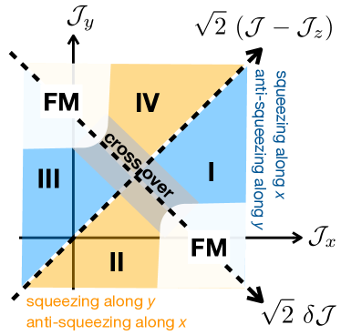
Figure 5: Sketch of the steady-state phase diagram of the dissipative XYZ model, indicating the squeezed/anti-squeezed collective-spin components predicted by perturbation theory.

On the other hand, the pure-state perturbation picture predicts that the perturbed state has the simple form of a superposition of two Dicke states:

$$|\phi_{0}^{\prime}\rangle\approx |J=N/2,M=-N/2\rangle$$

$$+\zeta|J=N/2,M=-N/2+2\rangle$$ (50)

such that

$$\langle\phi_{0}^{\prime}|S_{i}^{x}S_{j}^{x}|\phi_{0}^{\prime}\rangle =\zeta^{\prime}$$

$$\langle\phi_{0}^{\prime}|S_{i}^{y}S_{j}^{y}|\phi_{0}^{\prime}\rangle =-\zeta^{\prime}$$ (51)

where $\zeta^{\prime}=\zeta/\sqrt{2N(N-1)}$ . Given that

$$\zeta=-\frac{\sqrt{2N(N-1)}}{4(N-2)}\frac{\delta{\cal J}}{{\cal J}-{\cal J}^{z}}$$ (52)

we obtain positive, ferromagnetic correlations (and anti-squeezing) for the $x$ spin component when ${\delta{\cal J}}<0,{{\cal J}-{\cal J}^{z}}>0$ or ${\delta{\cal J}}>0,{{\cal J}-{\cal J}^{z}}<0$ (quadrants II and IV respectively), while negative correlations (ans squeezing) appear for the $y$ spin component. On the other hand, for ${\delta{\cal J}}>0,{{\cal J}-{\cal J}^{z}}>0$ and ${\delta{\cal J}}<0,{{\cal J}-{\cal J}^{z}}<0$ (quadrants I and III respectively) ferromagnetic correlations appear for the $y$ spin component etc. This is in agreement with the previous analysis of the extremizing angle. The picture of the correlation structure is summarized in Fig. 5.

Figure 6: Minimal spin squeezing parameter $\xi_{\rm R}^{2}$ in the dissipative TFI model as a function of $\mathcal{J}_{x}$ for the exact solution (full black line) and the perturbative solution (dashed orange line). Inset: the angle $\phi_{min}$ for which the spin squeezing parameter is minimal. Parameters used are $N=20$,$\Delta=-6\gamma$ (as indicated on the figure).

6.2 Example II: the dissipative transverse field Ising model

In the following we discuss a second model with two-emitter driving, namely the transverse-field Ising (TFI) model with collective (or infinite-dimensional) interactions and spontaneous local emission along the field axis [11], whose Hamiltonian is given by

$$H=\frac{{\cal J}_{x}}{N}\sum_{i,j}S_{i}^{x}S_{j}^{x}+\Delta\sum_{i}S_{i}^{z}\leavevmode\nobreak\ .$$ (53)

The dissipation is the same as for the previous model, namely we have single-emitter jump operators $L_{j}\to S_{i}^{-}$ with uniform single-emitter decay rate $\gamma$.

The Hamiltonian $H$ can be decomposed as a U(1)-symmetric unperturbed term and a symmetry-breaking perturbation ${H}=H_{0}+\lambda H_{1}$, with

$$H_{0}=\Delta J^{z},$$ (54)

and

$$\lambda H_{1} =\frac{{\cal J}_{x}}{N}\sum_{i,j}S_{i}^{x}S_{j}^{x}$$ (55)

$$=\frac{{\cal J}_{x}}{4N}\left[(J^{+})^{2}+(J^{-})^{2}+J^{+}J^{-}+J^{-}J^{+}\right]\leavevmode\nobreak\ .$$

The unique steady state $|\phi_{0}\rangle$ in the unperturbed limit $\lambda=0$ is, as before, the coherent spin state aligned with the $-z$ axis. And, as in the previous example, it is connected by the perturbation $H_{1}$ to only one eigenstate of the unperturbed Hamiltonian, namely the Dicke state $|\phi_{2}\rangle=|J=N/2,M=-N/2+2\rangle$. Since Dicke states have the unperturbed energies $E(J=N/2,M)=\Delta M$, the energy difference entering in the denominator of the first-order correction to the steady state, Eq. (12), is simply $E_{2}-E_{0}=2\Delta$.

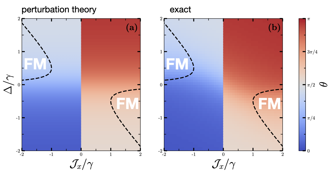
Figure 7: Optimal angle $\theta$ in the $(x,y)$-plain that minimises the spin squeezing parameter in the TFI model as predicted by (a) the perturbative approach and (b) the exact solution for a system with $N=20$. Black dashed lines show the mean-field phase transition between the paramagnetic phase and ferromagnetic phase.

Figure 8: Sketch of the steady-state phase diagram of the dissipative TFI model, indicating the squeezed/anti-squeezed collective-spin components predicted by perturbation theory.

The matrix element in the numerator of the first-order correction to the steady state reads instead

$$\langle\phi_{2}|H_{1}|\phi_{0}\rangle =\frac{{\cal J}_{x}}{4N}\left\langle\phi_{2}\right|(J^{+})^{2}\left|\phi_{0}\right\rangle,$$ (56)

$$=\frac{{\cal J}_{x}}{4}\sqrt{\frac{2\left(N-1\right)}{N}}\leavevmode\nobreak\ .$$ (57)

As a consequence the $F$ function entering in the squeezing parameter reads

$$F(\{\theta_{i}\})=\frac{e^{i2\theta}}{8}\frac{{\cal J}_{x}(N-1)}{2\Delta-i\gamma}=\frac{\alpha e^{i2\theta}}{\beta-i\gamma},$$ (58)

where $\alpha$ and $\beta$ are given by

$$\alpha =\frac{1}{8}{\cal J}_{x}(N-1)$$ (59)

$$\beta =2\Delta\leavevmode\nobreak\ .$$ (60)

The $F$ function has the same form as for the XYZ model, Eq. (43), and therefore the angle $\theta$ extremizing it and the corresponding extremal value have the same expression as those in Eqs. (48) and (49). As a consequence, for any (finite) value of the perturbation ${\cal J}_{x}$ and of the field $\Delta$ one can always find an angle $\theta$ for which squeezing appears. Fig. 6 shows an example of the optimal squeezing parameter and optimal angle for a system with $N=20$ spins, and for a field with strength $\Delta=-6\gamma$. The pure-state perturbation results capture the linear onset of squeezing upon adding a finite ${\cal J}_{x}$ perturbation. The agreement with the exact result – obtained again with the technique developed in Ref. [15] – degrades upon increasing the perturbation because the steady state develops some finite entropy, and most importantly because the system can experience a phase transition to ferromagnetism [11] (see Fig. 8 for a sketch of the phase diagram).

The full dependence of the squeezing angle on the Hamiltonian parameters ${\cal J}_{x}$ and $\Delta$, and on the dissipation strength $\gamma$, is shown in Fig. 7. To understand the main features of the angle map across the phase diagram, we can extract the optimal squeezing angle simply by taking the limit of negligible dissipation ($|\gamma/\beta|\ll 1$) in Eq. (47), which gives ${\rm Re}F\approx\alpha\cos(2\theta)/\beta$. This implies that $\theta=0\leavevmode\nobreak\ ({\rm mod}\leavevmode\nobreak\ \pi)$ is the optimal squeezing angle if $\alpha/\beta>0$, i.e. if $\Delta>0$ and ${\cal J}_{x}>0$, or $\Delta<0$ and ${\cal J}_{x}<0$ (quadrants I and III in the $({\cal J}_{x},\Delta)$ plane – see Fig. 8); while $\theta=\pi/2\leavevmode\nobreak\ ({\rm mod}\leavevmode\nobreak\ \pi)$ is the optimal squeezing angle in the two complementary quadrants $\Delta>0$ and ${\cal J}_{x}<0$, or $\Delta<0$ and ${\cal J}_{x}>0$ (quadrants II and IV respectively). The presence of a finite dissipation $\gamma$ introduces a smooth crossover in the squeezing angle between quadrant I and quadrant II, and between quadrant III and quadrant IV. Fig. 8 summarizes the structure of correlations (i.e. the squeezed vs. anti-squeezed collective-spin component) across the phase diagram of the system.

7 Single-emitter drive and second order perturbation theory

In this section we consider the most elementary form of drive which perturbs a dissipative system of emitters out of the state with all emitters in the ground state – namely single-emitter (or Rabi) drive. This generically corresponds to a perturbation in the form

$$\lambda{H}_{1}=-\frac{1}{2}\sum_{i}\Omega_{i}\left(e^{i\phi_{i}}S_{i}^{+}+e^{-i\phi_{i}}S_{i}^{-}\right)$$ (61)

where $\Omega_{i}$ is the local amplitude of the Rabi drive at site $i$, and $\phi_{i}$ the local phase.

The state perturbed by $H_{1}$ to first order experiences a net rotation of the collective spin away from the $z$ axis, but it remains a coherent spin state without any form of correlations. Indeed the first-order perturbed state is a superposition between the unperturbed state $|\phi_{0}\rangle\in{\cal S}_{-N/2}$ and a state in the magnetization sector with $M=-N/2+1$, $|\phi_{1}\rangle\in{\cal S}_{-N/2+1}$, so that $\langle\phi_{1}|S_{i}^{+}S_{j}^{-}|\phi_{0}\rangle=\langle\phi_{1}|S_{i}^{+}S_{j}^{+}|\phi_{0}\rangle=0$ for any $i\neq j$. To observe correlations one needs the superposition of $|\phi_{0}\rangle$ with a state $|\phi_{2}\rangle$ in the magnetization sector ${\cal S}_{-M/2+2}$, which can only be achieved at second order in the perturbation. Moreover the appearance of correlations requires also an interacting unperturbed Hamiltonian and/or collective emission, given that otherwise the state of the emitters remains perfectly factorized as in the unperturbed case.

In the following we apply the results of Sec. 2 for second-order perturbation theory to the relevant example of the driven Dicke model.

7.1 Example: the driven Dicke model

The driven Dicke model [46, 47] describes a symmetric coupling between the emitters and their environment, with a jump operator $\sqrt{\Gamma/N}J^{-}$. The emitters are driven away from their ground state by a uniform Rabi field along e.g. the $x$-direction, namely the unperturbed Hamiltonian is vanishing, $H_{0}=0$, while the perturbing Hamiltonian simply reads:

$$\lambda H_{1}=-\Omega J^{x}\leavevmode\nobreak\$$ (62)

namely it is of the form of Eq. (61) with uniform $\Omega_{i}=\Omega$ and $\phi_{i}=0$.

As already pointed out above, within first-order perturbation theory only the average collective spin can rotate, but correlations cannot appear; while they appear instead to second order. Applying Eqs. (12) and (13) we obtain for the perturbed state the form:

$$|\phi_{0}^{\prime}\rangle=\left(1-\frac{N\Omega^{2}}{2\Gamma^{2}}\right)\left|-\frac{N}{2}\right\rangle+\frac{i\Omega\sqrt{N}}{\Gamma}\left|-\frac{N}{2}+1\right\rangle$$

$$-\frac{\Omega^{2}N^{2}}{\Gamma^{2}\sqrt{2N(N-1)}}\left|-\frac{N}{2}+2\right\rangle+\mathcal{O}\left(\frac{\Omega^{3}}{\Gamma^{3}}\right)$$ (63)

where we have adopted the shorthand notation $|J=N/2,M\rangle\to|M\rangle$ for Dicke states. Expressions for various expectation values with respect to $|\phi^{\prime}_{0}\rangle$ can be found in App. B. We would like to point out that the collective emission plays a crucial role in keeping the perturbed state in the symmetric Dicke manifold, thereby allowing for the appearance of correlations, as the Dicke states are generically entangled except for the fully polarized ones. If the emission were not fully collective, the last term in Eq. (13) would admix the unperturbed state with states going out of the symmetric manifold.

The perturbed state develops a rotated net collective spin

$$\langle{\bm{J}}\rangle=\frac{N}{2}(0,\cos\phi,\sin\phi)=\frac{N}{2}\bm{e}_{\phi}$$ (64)

where

$$\cos\phi =-\frac{2\Omega}{\Gamma}+\mathcal{O}\left(\frac{\Omega^{3}}{\Gamma^{3}}\right)$$

$$\sin\phi =-\left(1-\frac{2\Omega^{2}}{\Gamma^{2}}\right)+\mathcal{O}\left(\frac{\Omega^{3}}{\Gamma^{3}}\right)\leavevmode\nobreak\ .$$ (65)

The squeezed component of the collective spin must therefore be searched for in the plane transverse to this rotated collective spin, namely as

$$J^{\theta}=\cos\theta\leavevmode\nobreak\ J^{x}+\sin\theta J^{\phi^{\prime}}\leavevmode\nobreak\$$ (66)

where $J^{\phi^{\prime}}=-\sin\phi\leavevmode\nobreak\ J^{y}+\cos\phi\leavevmode\nobreak\ J^{z}$ is the collective spin component orthogonal to $\bm{e}_{\phi}$ in the $yz$ plane.

By construction $J^{\theta}$ is orthogonal to the net orientation of the collective spin, and therefore $\langle J^{\theta}\rangle=\langle J^{x}\rangle=\langle J^{\phi^{\prime}}\rangle=0$. On the other hand

$$\langle(J^{\theta})^{2}\rangle =\cos^{2}\theta\leavevmode\nobreak\ \langle(J^{x})^{2}\rangle+\sin^{2}\theta\leavevmode\nobreak\ \langle(J^{\phi^{\prime}})^{2}\rangle$$

$$+\cos\theta\sin\theta\leavevmode\nobreak\ \langle J^{x}J^{\phi^{\prime}}+J^{\phi^{\prime}}J^{x}\rangle\leavevmode\nobreak\ .$$ (67)

One finds that $\langle J^{x}J^{\phi^{\prime}}+J^{\phi^{\prime}}J^{x}\rangle=0$ for the perturbed state in Eq. (63). To evaluate the rest of the above expression, after a lengthy but straightforward calculation one can show that

$$\langle(J^{x})^{2}\rangle=\frac{N}{4}-\frac{N\Omega^{2}}{2\Gamma^{2}}+\mathcal{O}\left(\frac{\Omega^{3}}{\Gamma^{3}}\right)$$ (68)

and

$$\langle(J^{\phi^{\prime}})^{2}\rangle=\frac{N}{4}+\frac{N\Omega^{2}}{2\Gamma^{2}}+\mathcal{O}\left(\frac{\Omega^{3}}{\Gamma^{3}}\right)\leavevmode\nobreak\ .$$ (69)

Hence we find that the $J^{x}$ fluctuations are squeezed below the projection noise $N/4$, while those of $J^{\phi^{\prime}}$ are anti-squeezed. In fact these collective spin components correspond to those maximizing (resp. minimizing) the squeezing parameter, since

$$\xi_{R}^{2} =\frac{N\leavevmode\nobreak\ {\rm Var}(J^{\theta})}{\langle\bm{J}\rangle^{2}}$$

$$=1+\frac{2\Omega^{2}}{\Gamma^{2}}\left(\sin^{2}\theta-\cos^{2}\theta\right)$$ (70)

which is clearly minimized for $\theta=0$, namely the maximally squeezed spin component corresponds to $J^{x}$. Moreover, we observe that

$$\langle(J^{x})^{2}\rangle\langle(J^{\phi^{\prime}})^{2}\rangle=\frac{|\langle\bm{J}\rangle|^{2}}{4}+\mathcal{O}\left(\frac{\Omega^{3}}{\Gamma^{3}}\right)$$ (71)

namely the squeezed state is again of minimal uncertainty.

The results for the minimal spin squeezing parameter ($\theta=0$) from second-order perturbation theory are compared to the exact results in Fig. 9. The second-order approach reproduces the quadratic onset of squeezing as a function of the drive $\Omega$, and follows its quadratic development for a rather broad parameter range – roughly equaling half of the extension of the paramagnetic phase in the steady state. Second order perturbation theory clearly breaks down on approach to the super-radiant transition [46, 47], occurring for $\Omega/\Gamma=1/2$.

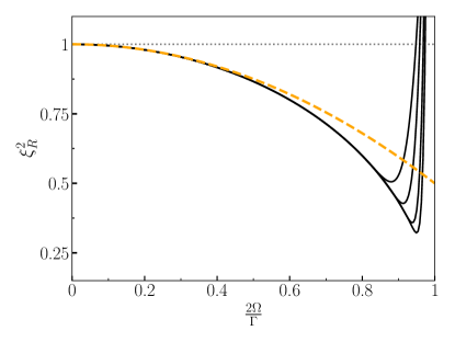
Figure 9: Minimal spin squeezing parameter $\xi_{\rm R}^{2}$ in the dissipative TFI model as a function of $\frac{2\Omega}{\Gamma}$. The black lines show the exact solutions for $N=50,100,200,300$ (decreasing minimum as $N$ increases). The orange dashed line shows the result of the second order perturbative approach.

8 Discussion

Throughout this work we have shown that spin squeezing is a form of quantum correlations which is promoted by the interplay between Hamiltonian driving and dissipation, either in the form of individual emission or of collective emission. A few previous works already identified squeezing as a characteristic feature of steady states in driven-dissipative quantum systems. In particular Ref. [8] found squeezing in the paramagnetic phase of the dissipative XYZ model on two- and three-dimensional lattices and nearest-neighbor interactions by evaluating Gaussian quantum fluctuations around the mean-field steady state. This result has been confirmed in Ref. [10] for the two-dimensional dissipative XYZ model, by making use of a truncated cumulant expansion of quantum fluctuations for each pure state within a quantum-trajectory approach to the driven dissipative dynamics. Spin squeezing in the paramagnetic steady state of the driven Dicke model has been previously reported in Ref. [47]. Our work encompasses all these results for weak driving, by defining the general conditions under which squeezing is expected in the paramagnetic phase, close to the trivial (i.e. undriven) steady state.

All of the applications we discussed in this work focus on collective-spin models (namely on Hamiltonians $H_{0}$ and $H_{1}$ only depending on the collective spin operator ${\bm{J}}$); yet the results we presented arguably apply to a much broader class of models. As discussed in Sec. 3.2, first- and second-order perturbation theory starting from the coherent spin state $|\phi_{0}\rangle$ can only produce states with $J\geq N/2-2$. Hence both the unperturbed Hamiltonian $H_{0}$ as well as its perturbation $H_{1}$ act on the states of interest as projected onto this large-spin sector of Hilbert space

$$H_{0(1)}\to H^{\rm(eff)}_{0(1)}={\cal P}_{J\geq N/2-2}\leavevmode\nobreak\ H_{0(1)}\leavevmode\nobreak\ {\cal P}_{J\geq N/2-2}$$ (72)

where ${\cal P}_{J\geq N/2-2}$ is the projector on the sector with $J\geq N/2-2$. Regardless of the range of interactions in $H_{0(1)}$, the projected Hamiltonians $H^{\rm(eff)}_{0(1)}$ have effectively long-range interactions. As an example, the Hamiltonian projected onto the sector with maximal $J=N/2$ has only infinite-range interactions (namely it depends only on the ${\bm{J}}$ operator). Therefore the physics of the collective-spin models explored in this work applies in fact also to their short-range-interacting versions, as long as one focuses on perturbative effects close to the $U(1)$ symmetric limit.

Single-emitter driving as in the driven Dicke model is obviously very relevant to experiments, as it is obtained by coupling the emitters to a Rabi field. The physics of the driven Dicke model has been recently realized experimentally in Ref. [25], and one can therefore expect squeezing to be a feature of the steady state at weak driving, and possibly up to the super-radiant transition. On the other hand, the experimental relevance of two-emitter driving is less obvious. Nonetheless, as discussed in Ref. [8], two-emitter driving can be realized by coupling pairs of emitters to pairs of lasers that are strongly detuned from single-emitter transitions, but are instead resonant for two-photon two-emitter transitions.

9 Conclusions

In this work we have introduced pure-state perturbation theory for the steady state of open quantum systems, valid when the system Hamiltonian is perturbed away from a known limit admitting a pure state as steady state. The assumption of a pure perturbed state allows for closed expressions of the coefficient of the perturbed state on the unperturbed Hamiltonian eigenbasis, and particularly so when the non-Hermitian Hamiltonian of the open quantum system is diagonalized by the eigenbasis of the unperturbed Hamiltonian.

Pure-state perturbation theory offers a significant insight into the physical properties of the perturbed steady state, in particular for what concerns quantum correlations. In this work we have focused our attention on ensembles of light emitters – i.e. qubits or (artificial) atoms – and we characterized quantum correlations by considering collective-spin properties, in particular the uncertainty of its components perpendicular to the average orientation. For ensembles of light emitters which emit photons individually, we could formulate a theorem for the onset of spin squeezing under the effect of two-emitter driving, based on first-order perturbation theory. The theorem applies to relevant models of collective interactions among emitters, i.e. the dissipative XYZ model [38] and the dissipative transverse-field Ising model [11] with all-to-all couplings. Furthermore we showed that single-emitter drive, in the form of Rabi coupling, leads to spin squeezing when the emitters are collectively coupled to the environment, as modeled by the driven Dicke model. Perturbation theory allows for explicit expressions of the perturbed states, and it shows that the spin-squeezed states are of minimal uncertainty, namely spin squeezing is their optimal resource for metrology, since the inverse spin-squeezing parameter coincides with the quantum Fisher information.

Our pure-state perturbation results are tested against exact results, and they exhibit a rather large domain of accuracy away from the unperturbed limit, validating the pure-state assumption. The near purity, or low entropy, of the perturbed state allows the Hamiltonian perturbation to induce quantum correlations in the steady state. It is important to point out that the low entropy of the steady state is actually a condition valid when the dissipation is much stronger than the drive, keeping the system close to the (pure) ground state of each emitter. The fast dissipation prevents the emitters from being highly excited and therefore from radiating significantly into the environment – something which would entail instead a significant entropy in the steady state. Hence the form of quantum correlations described in this work are the result of a very specific interplay between dissipation and drive, resulting in the so-called normal phase within the steady-state phase diagram. This can be contrasted with the super-radiant phase, developing long-range correlations among the emitters, but also a large entropy due to the important emission of radiation into the environment.

The perturbative approach allows for analytical predictions of the steady state and its quantum correlation properties when the system is weakly driven. But, more generally, the predictions of perturbation theory provide a significant insight into the mechanisms leading to the appearance of the specific correlation patterns of the steady state, which can characterize the phase diagram beyond the strict limit of applicability of the perturbative approach. This is crucial in the absence of a simple variational principle – such as the minimization of the free energy – which dictates the form of the steady state, and which could allow for an intuitive (e.g. semiclassical) prediction of its properties. A relevant example provided in this work is offered by the appearance of ferromagnetic correlations in the steady state of the dissipative XYZ model, in spite of the Hamiltonian interactions being antiferromagnetic; and the fact that the most correlated spin components are not necessarily those which are most strongly interacting. These predictions go clearly beyond what one can reconstruct via mean-field theory, which pictures the whole paramagnetic phase as being identical to the U(1)-symmetric steady state [38]. The insight acquired via perturbation theory can be used as a precious guidance in the understanding and the design of many-body quantum states resulting from the competition between strong dissipation and a weak drive; and it can be applied rather broadly to dissipative quantum many-body systems. In this work we focused on ensembles of light emitters, relevant to a very broad spectrum of physical systems ranging from atomic physics (e.g. Rydberg atoms [8], atomic ensembles close to the super-radiant transition [47, 25], etc.) to solid-state physics [24]. Yet it is clear that one can apply the same scheme to different degrees of freedom – e.g. to coupled bosonic modes leaking into the environment, and close to their vacuum state.

Appendix A Calculation of ${\rm Re}\left[F(\left\{\theta_{\rm ex}\right\})\right]$

In this section we detail the calculations of the function ${\rm Re}\left[F(\left\{\theta_{\rm ex}\right\})\right]$ appearing in theorem 1, assuming that its real part can be written in the form of Eq. (47). That is, one can write

$${\rm Re}\left[F(\left\{\theta_{\rm ex}\right\})\right]=\frac{\alpha\left(\beta\cos 2\theta_{\rm ex}-\gamma\sin 2\theta_{\rm ex}\right)}{\beta^{2}+\gamma^{2}}.$$ (73)

The angle $\theta_{\rm ex}$ extremizing the function leads to a vanishing derivative of Eq. (73) with respect to $\theta$ to zero. The result of Eq. (48) is then obtained as follows

$$\frac{d}{d\theta}{\rm Re}[F(\{\theta\})]=0\leavevmode\nobreak\ \leavevmode\nobreak\ \leavevmode\nobreak\ \leavevmode\nobreak\ \Leftrightarrow\leavevmode\nobreak\ \leavevmode\nobreak\ \leavevmode\nobreak\ \leavevmode\nobreak\ \tan 2\theta=-\frac{\gamma}{\beta}\leavevmode\nobreak\ \leavevmode\nobreak\ \leavevmode\nobreak\ \leavevmode\nobreak\ \Leftrightarrow\leavevmode\nobreak\ \leavevmode\nobreak\ \leavevmode\nobreak\ \leavevmode\nobreak\ \theta_{ex}=\frac{1}{2}\tan^{-1}\left(-\frac{\gamma}{\beta}\right)+k\frac{\pi}{2}\quad k\in\mathbb{Z}.$$ (74)

We can now substitute this result in Eq. (73), and calculate for which angle ${\rm Re}\left[F(\left\{\theta_{\rm ex}\right\})\right]>0$, i.e. spin squeezing occurs. This yields

$${\rm Re}\left[F(\left\{\theta_{\rm ex}\right\})\right]=\frac{\alpha\left[\beta\cos\left(\tan^{-1}\left(-\frac{\gamma}{\beta}\right)+k\pi\right)-\gamma\sin\left(\tan^{-1}\left(-\frac{\gamma}{\beta}\right)+k\pi\right)\right]}{\beta^{2}+\gamma^{2}}\leavevmode\nobreak\ .$$ (75)

We can simplify this expression via standard trigonometric formulas, and using the fact that $\cos(\tan^{-1}(x))=\frac{1}{\sqrt{1+x^{2}}}$ and $\sin(\tan^{-1}(x))=\frac{x}{\sqrt{1+x^{2}}}$. Hence,

$$\cos\left(\tan^{-1}\left(-\frac{\gamma}{\beta}\right)+k\pi\right)=\frac{\cos(k\pi)}{\sqrt{1+\frac{\gamma^{2}}{\beta^{2}}}},$$ (76)

and

$$\sin\left(\tan^{-1}\left(-\frac{\gamma}{\beta}\right)+k\pi\right)=\frac{-\frac{\gamma}{\beta}}{\sqrt{1+\frac{\gamma^{2}}{\beta^{2}}}}\cos\left(k\pi\right).$$ (77)

Substituting this result in Eq. (75) finally allows us to write

$${\rm Re}\left[F(\left\{\theta_{\rm ex}\right\})\right]=\frac{\alpha\left[\beta^{2}\frac{\cos(k\pi)}{\sqrt{\beta^{2}+\gamma^{2}}}+\gamma^{2}\frac{\cos\left(k\pi\right)}{\sqrt{\beta^{2}+\gamma^{2}}}\right]}{\beta^{2}+\gamma^{2}}=\frac{\alpha\cos(k\pi)}{\sqrt{\beta^{2}+\gamma^{2}}}.$$ (78)

Appendix B Perturbation-theory predictions for the driven Dicke model

In this section we provide the reader with a list of the results for the expectation values of collective spin operators, and products thereof, for the driven Dicke model discussed in Section 7.1, as obtained for the perturbed state $|\phi_{0}^{\prime}\rangle$ given in Eq. 63. After a straightforward calculation, one obtains up to second order in $\Omega/\Gamma$:

$$\langle\phi_{0}^{\prime}|J^{x}|\phi_{0}^{\prime}\rangle =0\leavevmode\nobreak\ ,$$ (79)

$$\langle\phi_{0}^{\prime}|J^{y}|\phi_{0}^{\prime}\rangle =-\frac{\Omega N}{\Gamma}\leavevmode\nobreak\ ,$$ (80)

$$\langle\phi_{0}^{\prime}|J^{z}|\phi_{0}^{\prime}\rangle =-\frac{N}{2}+\frac{\Omega^{2}N}{\Gamma^{2}}\leavevmode\nobreak\ ,$$ (81)

$$\langle\phi_{0}^{\prime}|J^{z}|\phi_{0}^{\prime}\rangle^{2} =\frac{N^{2}}{4}-\frac{\Omega^{2}N^{2}}{\Gamma^{2}}\leavevmode\nobreak\ ,$$ (82)

$$\langle\phi_{0}^{\prime}|\left(J^{x}\right)^{2}|\phi_{0}^{\prime}\rangle =\frac{N}{4}-\frac{\Omega^{2}N}{2\Gamma^{2}}\leavevmode\nobreak\ ,$$ (83)

$$\langle\phi_{0}^{\prime}|\left(J^{y}\right)^{2}|\phi_{0}^{\prime}\rangle =\frac{N}{4}+\frac{1}{2}\frac{\Omega^{2}}{\Gamma^{2}}N(2N-1)\leavevmode\nobreak\ ,$$ (84)

$$\langle\phi_{0}^{\prime}|\left(J^{z}\right)^{2}|\phi_{0}^{\prime}\rangle =\frac{N^{2}}{4}-\frac{\Omega^{2}}{\Gamma^{2}}N\left(N-1\right)\leavevmode\nobreak\ .$$ (85)

For the expressions of the form $\langle\phi_{0}^{\prime}|J^{\alpha}J^{\beta}|\phi_{0}^{\prime}\rangle+\langle\phi_{0}^{\prime}|J^{\beta}J^{\alpha}|\phi_{0}^{\prime}\rangle$ one finds

$$\langle\phi_{0}^{\prime}|J^{x}J^{y}|\phi_{0}^{\prime}\rangle+\langle\phi_{0}^{\prime}|J^{y}J^{x}|\phi_{0}^{\prime}\rangle =0\leavevmode\nobreak\ ,$$ (86)

$$\langle\phi_{0}^{\prime}|J^{x}J^{z}|\phi_{0}^{\prime}\rangle+\langle\phi_{0}^{\prime}|J^{z}J^{x}|\phi_{0}^{\prime}\rangle =0\leavevmode\nobreak\ ,$$ (87)

$$\langle\phi_{0}^{\prime}|J^{y}J^{z}|\phi_{0}^{\prime}\rangle+\langle\phi_{0}^{\prime}|J^{z}J^{y}|\phi_{0}^{\prime}\rangle =\frac{\Omega}{\Gamma}N\left(N-1\right)\leavevmode\nobreak\ .$$ (88)

References

- Frérot et al. [2023] I. Frérot, M. Fadel and M. Lewenstein, Probing quantum correlations in many-body systems: a review of scalable methods, Reports on Progress in Physics 86, 114001 (2023).
- Horodecki et al. [2009] R. Horodecki, P. Horodecki, M. Horodecki and K. Horodecki, Quantum Entanglement, Rev. Mod. Phys. 81, 865 (2009).
- Georgescu et al. [2014] I. M. Georgescu, S. Ashhab and F. Nori, Quantum simulation, Rev. Mod. Phys. 86, 153 (2014).
- Verstraete et al. [2009] F. Verstraete, M. M. Wolf and J. I. Cirac, Quantum computation and quantum-state engineering driven by dissipation, Nat. Phys. 5, 633 (2009).
- Diehl et al. [2008] S. Diehl, A. Micheli, A. Kantian, B. Kraus, H. P. Büchler and P. Zoller, Quantum states and phases in driven open quantum systems with cold atoms, Nat. Phys. 4, 878 (2008).
- Weimer et al. [2010] H. Weimer, M. Müller, I. Lesanovsky, P. Zoller and H. P. Büchler, A Rydberg quantum simulator, Nature Physics 6, 382 (2010).
- Müller et al. [2012] M. Müller, S. Diehl, G. Pupillo and P. Zoller, Engineered Open Systems and Quantum Simulations with Atoms and Ions, Adv. At. Mol. Opt. Phys. 61, 1 (2012).
- Lee et al. [2013] T. E. Lee, S. Gopalakrishnan and M. D. Lukin, Unconventional Magnetism via Optical Pumping of Interacting Spin Systems, Phys. Rev. Lett. 110, 257204 (2013).
- Jin et al. [2016] J. Jin, A. Biella, O. Viyuela, L. Mazza, J. Keeling, R. Fazio and D. Rossini, Cluster Mean-Field Approach to the Steady-State Phase Diagram of Dissipative Spin Systems, Phys. Rev. X 6, 031011 (2016).
- Verstraelen et al. [2023] W. Verstraelen, D. Huybrechts, T. Roscilde and M. Wouters, Quantum and Classical Correlations in Open Quantum Spin Lattices via Truncated-Cumulant Trajectories, PRX Quantum 4, 030304 (2023).
- Overbeck et al. [2017] V. R. Overbeck, M. F. Maghrebi, A. V. Gorshkov and H. Weimer, Multicritical behavior in dissipative Ising models, Phys. Rev. A 95, 042133 (2017).
- Finazzi et al. [2015] S. Finazzi, A. Le Boité, F. Storme, A. Baksic and C. Ciuti, Corner-Space Renormalization Method for Driven-Dissipative Two-Dimensional Correlated Systems, Phys. Rev. Lett. 115, 080604 (2015).
- Weimer [2015] H. Weimer, Variational Principle for Steady States of Dissipative Quantum Many-Body Systems, Phys. Rev. Lett. 114, 040402 (2015).
- Sieberer et al. [2016] L. M. Sieberer, M. Buchhold and S. Diehl, Keldysh field theory for driven open quantum systems, Reports on Progress in Physics 79, 096001 (2016).
- Shammah et al. [2018] N. Shammah, S. Ahmed, N. Lambert, S. De Liberato and F. Nori, Open quantum systems with local and collective incoherent processes: Efficient numerical simulations using permutational invariance, Phys. Rev. A 98, 063815 (2018).
- Vicentini et al. [2019] F. Vicentini, A. Biella, N. Regnault and C. Ciuti, Variational Neural-Network Ansatz for Steady States in Open Quantum Systems, Phys. Rev. Lett. 122, 250503 (2019).
- Nagy and Savona [2019] A. Nagy and V. Savona, Variational Quantum Monte Carlo Method with a Neural-Network Ansatz for Open Quantum Systems, Phys. Rev. Lett. 122, 250501 (2019).
- Hartmann and Carleo [2019] M. J. Hartmann and G. Carleo, Neural-Network Approach to Dissipative Quantum Many-Body Dynamics, Phys. Rev. Lett. 122, 250502 (2019).
- Weimer et al. [2021] H. Weimer, A. Kshetrimayum and R. Orús, Simulation methods for open quantum many-body systems, Rev. Mod. Phys. 93, 015008 (2021).
- Deuar et al. [2021] P. Deuar, A. Ferrier, M. Matuszewski, G. Orso and M. H. Szymanska, Fully Quantum Scalable Description of Driven-Dissipative Lattice Models, PRX Quantum 2, 010319 (2021).
- Mink et al. [2022] C. D. Mink, D. Petrosyan and M. Fleischhauer, Hybrid discrete-continuous truncated Wigner approximation for driven, dissipative spin systems, arXiv preprint arXiv:2203.17120 (2022).
- Reitz et al. [2022] M. Reitz, C. Sommer and C. Genes, Cooperative Quantum Phenomena in Light-Matter Platforms, PRX Quantum 3, 010201 (2022).
- Pezzè et al. [2018] L. Pezzè, A. Smerzi, M. K. Oberthaler, R. Schmied and P. Treutlein, Quantum metrology with nonclassical states of atomic ensembles, Rev. Mod. Phys. 90, 035005 (2018).
- Cong et al. [2016] K. Cong, Q. Zhang, Y. Wang, G. T. Noe, A. Belyanin and J. Kono, Dicke superradiance in solids, J. Opt. Soc. Am. B 33, C80 (2016).
- Ferioli et al. [2021] G. Ferioli, A. Glicenstein, F. Robicheaux, R. T. Sutherland, A. Browaeys and I. Ferrier-Barbut, Laser-Driven Superradiant Ensembles of Two-Level Atoms near Dicke Regime, Phys. Rev. Lett. 127, 243602 (2021).
- Breuer and Petruccione [2007] H. Breuer and F. Petruccione, The Theory of Open Quantum Systems (OUP Oxford, 2007).
- Benatti et al. [2011] F. Benatti, A. Nagy and H. Narnhofer, Asymptotic entanglement and Lindblad dynamics: a perturbative approach, Journal of Physics A: Mathematical and Theoretical 44, 155303 (2011).
- Li et al. [2014] A. C. Y. Li, F. Petruccione and J. Koch, Perturbative approach to Markovian open quantum systems, Scientific Reports 4, 4887 (2014).
- Li et al. [2016] A. C. Y. Li, F. Petruccione and J. Koch, Resummation for Nonequilibrium Perturbation Theory and Application to Open Quantum Lattices, Phys. Rev. X 6, 021037 (2016).
- Gómez et al. [2018] E. A. Gómez, J. D. Castaño-Yepes and S. P. Thirumuruganandham, Perturbation theory for open quantum systems at the steady state, Results in Physics 10, 353 (2018).
- Lenarčič et al. [2018] Z. Lenarčič, F. Lange and A. Rosch, Perturbative approach to weakly driven many-particle systems in the presence of approximate conservation laws, Phys. Rev. B 97, 024302 (2018).
- Kato [1995] T. Kato, Perturbation theory for linear operators, Classics in Mathematics (Springer, 1995).
- Landau and Lifshitz [1981] L. Landau and E. Lifshitz, Quantum Mechanics: Non-Relativistic Theory, Course of Theoretical Physics, Vol. 3 (Elsevier Science, 1981).
- Wineland et al. [1994] D. J. Wineland, J. J. Bollinger, W. M. Itano and D. J. Heinzen, Squeezed atomic states and projection noise in spectroscopy, Phys. Rev. A 50, 67 (1994).
- Sørensen et al. [2001] A. Sørensen, L.-M. Duan, J. I. Cirac and P. Zoller, Many-particle entanglement with Bose–Einstein condensates, Nature 409, 63 (2001).
- Braunstein and Caves [1994] S. L. Braunstein and C. M. Caves, Statistical distance and the geometry of quantum states, Phys. Rev. Lett. 72, 3439 (1994).
- Roscilde et al. [2021] T. Roscilde, F. Mezzacapo and T. Comparin, Spin squeezing from bilinear spin-spin interactions: Two simple theorems, Phys. Rev. A 104, L040601 (2021).
- Huybrechts et al. [2020] D. Huybrechts, F. Minganti, F. Nori, M. Wouters and N. Shammah, Validity of mean-field theory in a dissipative critical system: Liouvillian gap, -symmetric antigap, and permutational symmetry in the model, Phys. Rev. B 101, 214302 (2020).
- Johansson et al. [2012] J. Johansson, P. Nation and F. Nori, QuTiP: An open-source Python framework for the dynamics of open quantum systems, Computer Physics Communications 183, 1760 (2012).
- Johansson et al. [2013] J. Johansson, P. Nation and F. Nori, QuTiP 2: A Python framework for the dynamics of open quantum systems, Computer Physics Communications 184, 1234 (2013).
- Rota et al. [2017] R. Rota, F. Storme, N. Bartolo, R. Fazio and C. Ciuti, Critical behavior of dissipative two-dimensional spin lattices, Phys. Rev. B 95, 134431 (2017).
- Rota et al. [2018] R. Rota, F. Minganti, A. Biella and C. Ciuti, Dynamical properties of dissipative XYZ Heisenberg lattices, New Journal of Physics 20, 045003 (2018).
- Huybrechts and Wouters [2019] D. Huybrechts and M. Wouters, Cluster methods for the description of a driven-dissipative spin model, Phys. Rev. A 99, 043841 (2019).
- Huybrechts and Roscilde [2024] D. Huybrechts and T. Roscilde, in preparation (2024).
- Carollo and Lesanovsky [2021] F. Carollo and I. Lesanovsky, Exactness of Mean-Field Equations for Open Dicke Models with an Application to Pattern Retrieval Dynamics, Phys. Rev. Lett. 126, 230601 (2021).
- Narducci et al. [1978] L. M. Narducci, D. H. Feng, R. Gilmore and G. S. Agarwal, Transient and steady-state behavior of collective atomic systems driven by a classical field, Phys. Rev. A 18, 1571 (1978).
- Hannukainen and Larson [2018] J. Hannukainen and J. Larson, Dissipation-driven quantum phase transitions and symmetry breaking, Phys. Rev. A 98, 042113 (2018).