A randomized algorithm for simultaneously diagonalizing symmetric matrices by congruence

Abstract

A family of symmetric matrices $A_{1},\ldots,A_{d}$ is SDC (simultaneous diagonalization by congruence) if there is an invertible matrix $X$ such that every $X^{T}A_{k}X$ is diagonal. In this work, a novel randomized SDC (RSDC) algorithm is proposed that reduces SDC to a generalized eigenvalue problem by considering two (random) linear combinations of the family. We establish exact recovery: RSDC achieves diagonalization with probability $1$ if the family is exactly SDC. Under a mild regularity assumption, robust recovery is also established: Given a family that is $\epsilon$-close to SDC then RSDC diagonalizes, with high probability, the family up to an error of norm ${\mathcal{O}}(\epsilon)$. Under a positive definiteness assumption, which often holds in applications, stronger results are established, including a bound on the condition number of the transformation matrix. For practical use, we suggest to combine RSDC with an optimization algorithm. The performance of the resulting method is verified for synthetic data, image separation and EEG analysis tasks. It turns out that our newly developed method outperforms existing optimization-based methods in terms of efficiency while achieving a comparable level of accuracy.

1 Introduction

A family of real symmetric $n\times n$ matrices $(A_{1},\ldots,A_{d})$ is called simultaneously diagonalizable by congruence (SDC) if there is an invertible matrix $X$ such that $X^{T}A_{k}X$ is diagonal [16, 28, 32]. Under the stronger assumption that $X$ is orthogonal, such a family is usually called jointly diagonalizable (JD), which is equivalent to assuming that it is commuting. In this work, we extend our previous study [27] on randomized methods for JD to SDC.

SDC problems arise in a wide range of applications. Classically, in Blind Source Separation (BSS) [18] signal reconstruction is performed by applying SDC to covariance matrices associated with the observed noisy signals. It also plays a crucial role in robust Canonical Polyadic (CP) decomposition of tensors, see for example [21, Algorithm 3.1]. Recent applications of SDC include transfer learning [42], remote sensing [29], and quadratic programming [28, 32].

Due to noise caused by, e.g., modeling, estimation or round-off errors, the SDC assumption is virtually never satisfied in practice. Instead, one encounters a family $(\tilde{A}_{1},\ldots,\tilde{A}_{d})=(A_{1}+\epsilon E_{1},\ldots,A_{d}+\epsilon E_{d})$ that is nearly SDC, that is, the members $A_{k}$ of an underlying (unknown) SDC family are perturbed by error matrices $\epsilon E_{k}$. Most existing algorithms for addressing such SDC problems proceed by considering an optimization problem of the form

$$\min_{\tilde{X}\text{ invertible}}\mathcal{L}(\tilde{X}),$$ (1.1)

where $\mathcal{L}(\tilde{X})$ is a suitable loss function measuring off-diagonality for each transformed matrix $\tilde{X}^{T}\tilde{A}_{k}\tilde{X}$. A natural choice is

$$\mathcal{L}(\tilde{X}):=\sum_{k=1}^{d}\big{\|}\operatorname{offdiag}(\tilde{X}^{T}\tilde{A}_{k}\tilde{X})\big{\|}^{2}_{F},$$ (1.2)

where $\operatorname{offdiag}(\cdot)$ sets the diagonal entries of a matrix to zero and $\|\cdot\|_{F}$ denotes the Frobenius norm. Various optimization methods, including a quasi-Newton method [43] and an alternating Gauss-Newton iteration [40] have been applied to this loss function. One obvious issue when working with (1.2) is that $\mathcal{L}(\tilde{X})$ can be made arbitrarily small by simply rescaling $\tilde{X}$. A popular strategy to bypass this problem is to additionally impose the constraint that $\tilde{X}$ is in the oblique manifold $\operatorname{\mathcal{OB}}(n,n)$, that is, each column of $\tilde{X}$ has Euclidean norm $1$. For example in [40], the columns of $\tilde{X}$ are renormalized after each iteration. Exploiting that $\operatorname{\mathcal{OB}}(n,n)$ forms a Riemannian manifold, one can apply Riemannian optimization techniques [3, 15] to SDC, such as Riemannian trust region [2], Riemannian BFGS [14] and Riemannian conjugate gradient [41, 12] methods.

When $\tilde{A}_{k}$ is not only symmetric but also positive definite, a popular choice [34] of the loss function is given by

$$\mathcal{L}(\tilde{X}):=\frac{1}{2n}\sum_{k=1}^{d}[\log\det\operatorname{diag}(\tilde{X}^{T}\tilde{A}_{k}\tilde{X})-\log\det(\tilde{X}^{T}\tilde{A}_{k}\tilde{X})],$$ (1.3)

where $\operatorname{diag}(A):=A-\operatorname{offdiag}(A)$. As this loss function is invariant under column scaling [34], no additional constraint needs to be imposed on $\tilde{X}$. In many signal processing applications [18], the positive definite assumption is implied by the fact that $\tilde{A}_{k}$ is a sample covariance matrix. In this situation, the loss function (1.3) can be interpreted as the KL-divergence between zero-mean multivariate Gaussian distributions with covariance matrices $\tilde{X}^{T}\tilde{A}_{k}\tilde{X}$ and $\operatorname{diag}(\tilde{X}^{T}\tilde{A}_{k}\tilde{X})$ [13]. In the original paper [34], the optimization problem (1.1) with loss function (1.3) is solved by a Jacobi-like method, successively applying invertible $2\times 2$ transformations acting on pairs of columns. In [1], a quasi-Newton method is proposed that uses an approximate Hessian of (1.3). In [14], a Riemannian optimization algorithm that optimizes (1.3) directly on the manifold of invertible matrices is developed and analyzed.

Optimization-based SDC algorithms enjoy two major advantages: Their convergence analysis inherits the theory of the underlying optimization algorithms [43, 40] and they can be easily modified to suit more specific applications [40, 33]. However, to the best of our knowledge, none of the existing methods is guaranteed to converge to the global minimum of (1.1). Moreover, as observed in [27], optimization-based algorithms are often significantly slower than methods that utilize well-tuned linear algebra software.

In this paper, we propose and analyze a novel randomized SDC (RSDC) algorithm that is not only simpler but often also significantly faster than optimization-based SDC algorithms. The core concept is simple: Similar to existing methods for JD [27, 23], for learning latent variable models [5, 6, 7], for robust CP decomposition tensors [25] and for joint Schur decomposition [20], we obtain $\tilde{X}$ by diagonalizing two random linear combinations of the matrices in the family. In contrast, existing work [24, 21] on SDC in the context of the CP decomposition utilizes two fixed matrices from the family. RSDC is straightforward to implement and exploits existing high-quality software for generalized eigenvalue problems implemented in, e.g., LAPACK [8, 30, 36]. Moreover, unlike optimization-based methods, RSDC comes with recovery guarantees: Given a family that is (exactly) SDC, RSDC returns, with probability one, a matrix $X$ that transforms the family to diagonal form by congruence. Given a well-behaved (the precise meaning will be clarified in Section 2) family that is nearly SDC, RSDC returns after column normalization, with high probability, an error (1.2) of ${\mathcal{O}}(\epsilon)$. Furthermore, the accuracy can be further improved by refining the output of RSDC with the quasi-Newton method from [43].

The rest of this paper is organized as follows: In Section 2, preliminaries about matrix pairs and families will be covered. In Section 3, the Randomized SDC (RSDC) algorithm is introduced and its exact recovery is established. In Section 4, the robust recovery of RSDC is established under certain regularity and positive definiteness assumptions. Section 5 covers important implementation details as well as the refinement of the output returned by RSDC. Section 6 showcases the accuracy and efficiency of our algorithms through extensive numerical experiments, comparing with several state-of-the-art SDC solvers on both synthetic data and applications.

2 Preliminaries

In this section, we discuss the basic properties of matrix families in the context of SDC.

For $d=2$, a matrix family becomes a matrix pair $(A,B)\in{\mathbb{R}}^{n\times n}\times{\mathbb{R}}^{n\times n}$, closely associated with the generalized eigenvalue problem [26, 37] for the matrix pencil $A-\lambda B$. Such a pair is called regular if the polynomial $\lambda\mapsto\det(A-\lambda B)$ does not vanish. If a symmetric matrix pair $(A,B)$ is regular and SDC then its Weierstrass canonical form [37, Chapter VI, Theorem 1.13] is always diagonal. This implies that regularity is not sufficient to ensure the SDC property for a symmetric matrix pair $(A,B)$. For example, consider

$$A=\begin{bmatrix}0&1\\ 1&\epsilon\end{bmatrix},\quad B=\begin{bmatrix}0&1\\ 1&0\end{bmatrix},\quad\epsilon\neq 0.$$ (2.1)

If there was an invertible matrix $X$ such that $X^{T}AX=D_{A}$, $X^{T}BX=D_{B}$ are diagonal, $X^{-1}B^{-1}AX=D_{B}^{-1}D_{A}$ is diagonal. However,

$$B^{-1}A=\begin{bmatrix}1&\epsilon\\ 0&1\end{bmatrix}$$

which is clearly not diagonalizable and leads to a contradiction. Thus $(A,B)$ is not SDC. The example (2.1) also shows that arbitrarily small perturbations can destroy the SDC property, as the pair is clearly SDC for $\epsilon=0$.

Let us now consider a family of $d\geq 2$ matrices: $A_{1},\ldots,A_{d}\in\mathbb{R}^{n\times n}$. Given a vector

of scalars $\mu\in\mathbb{R}^{d}$, we define

$$A(\mu):=\mu_{1}A_{1}+\ldots+\mu_{d}A_{d}.$$

In the following, we will now extend certain concepts, such as regularity, from matrix pairs to matrix families.

Definition 1.

A family $(A_{1},\ldots,A_{d})$ with $A_{k}\in{\mathbb{R}}^{n\times n}$ is called regular if $\mu\mapsto\det(A(\mu))$ does not vanish.

Because $\det(A(\mu))$ is polynomial in the entries of $\mu$, it follows that a family is regular if and only if $A(\mu)$ is invertible for almost every $\mu\in\mathbb{R}^{d}$.

It clearly holds for all $\mu$ that

$$\ker(A(\mu))\subseteq\ker(A_{1})\cap\cdots\cap\ker(A_{d}).$$ (2.2)

Thus, a necessary (but not sufficient) condition for regularity is that $\ker(A_{1})\cap\cdots\cap\ker(A_{d})=\{0\}$. The following lemma identifies two situations in which equality holds in (2.2). Here and in the following, ${\mathbb{R}}_{>0}^{d}$ denotes the set of vectors of length $d$ with positive entries.

Lemma 2.

1. Let $A_{1},\ldots,A_{d}$ be symmetric positive semidefinite. Then $\ker(A(\mu))=\ker(A_{1})\cap\cdots\cap\ker(A_{d})$ holds for any $\mu\in{\mathbb{R}}_{>0}^{d}$.

2. Let $(A_{1},\ldots,A_{d})$ be SDC. Then $\ker(A(\mu))=\ker(A_{1})\cap\cdots\cap\ker(A_{d})$ holds for almost every $\mu\in{\mathbb{R}}^{d}$.

Proof.

(i) To establish the other inclusion in (2.2), let $x\in\ker(A(\mu))$. Then $x^{T}A(\mu)x=\mu_{1}x^{T}A_{1}x+\ldots+\mu_{d}x^{T}A_{d}x=0.$ Because each $A_{k}$ is positive semidefinite and $\mu$ is positive, this implies $x^{T}A_{k}x=0$ and, in turn, $x\in\ker(A_{k})$ for every $k$.

(ii) Let $X$ be invertible such that $X^{T}A_{k}X=D_{k}$ is diagonal for $k=1,\ldots,d$. This implies $X^{T}A(\mu)X=D(\mu)$ and

$$\ker(A_{k})=X\ker(D_{k}),\quad\ker(A(\mu))=X\ker(D(\mu)).$$

For generic $\mu$, $D(\mu)$ has a zero diagonal entry if and only if all the corresponding diagonal entries of $D_{k}$ are zero as well. This shows $\ker(D(\mu))=\ker(D_{1})\cap\cdots\cap\ker(D_{d})$. ∎

The following definition is partly motivated by Lemma 2.

Definition 3.

A family $(A_{1},\ldots,A_{d})$ of symmetric matrices is called positive definite (PD) if $A(\mu)$ is positive definite for every $\mu\in{\mathbb{R}}_{>0}^{d}$.

For $d=2$, Definition 3 is stronger than the classical definition of a definite pair [37], which only requires the existence of at least one positive definite linear combination. Using Lemma 2, it follows that a family $(A_{1},\ldots,A_{d})$ is PD if and only if each $A_{k}$ is positive semidefinite and $\ker(A_{1})\cap\cdots\cap\ker(A_{d})=\{0\}$. Clearly, a PD family is also regular.

3 Exact recovery of SDC

3.1 Basic idea and template algorithm

In [4], it is explained why JD is generically a one-matrix problem, while SDC is generically a two-matrix problem. In analogy to our work on JD in [27, Algorithm 1], this suggests that one can hope to solve the SDC problem from two linear combinations. More formally, given a family $(A_{1},\ldots,A_{d})$ that is SDC, we form two random linear combinations

$$A(\mu)=\mu_{1}A_{1}+\ldots+\mu_{d}A_{d},\quad A(\theta)=\theta_{1}A_{1}+\ldots+\theta_{d}A_{d},$$

and find an invertible $X$ (if it exists) such that $X^{T}A(\mu)X$ and $X^{T}A(\theta)X$ are diagonal. This idea leads to the Randomized SDC (RSDC) summarized in Algorithm 1. Implementation details, especially concerning Line 3, will be covered in Section 5. We will establish exact and robust recovery of this algorithm in Sections 3.2 and 4, respectively.

Algorithm 1 Randomized Simultaneous Diagonalization via Congruence (RSDC)

Input: An SDC family $(A_{1},\ldots,A_{d})$.
Output: Invertible matrix $X$ such that $X^{T}A_{k}X$ is diagonal for $k=1,\ldots,d$.

1:  Draw $\mu,\theta\in\mathbb{R}^{d}$ from specified distributions.

2:  Compute $A(\mu)=\mu_{1}A_{1}+\cdots+\mu_{d}A_{d}$, $A(\theta)=\theta_{1}A_{1}+\cdots+\theta_{d}A_{d}$.

3:  Compute an invertible $X$ such that $X^{T}A(\mu)X$ and $X^{T}A(\theta)X$ are diagonal.

4:  return  $X$

3.2 Exact recovery

Trivially, any pair of linear combinations $(A(\mu),A(\theta))$ of an SDC family is also SDC. It turns out that a congruence transformation diagonalizing this pair almost always diagonalizes the whole family. To show this, we exploit an existing connection between SDC and JD or, equivalently, commutativity.

Lemma 4 ([32, Theorem 3.1 (ii)]).

A family $(A_{1},\ldots A_{d})$ of symmetric matrices is SDC if and only if there is an invertible matrix $P$ such that $(P^{T}A_{1}P,\ldots,P^{T}A_{d}P)$ is a commuting family.

Remark 5.

If there is a positive definite linear combination $A(\theta)$ and, hence, $A(\theta)=LL^{T}$ admits a Cholesky factorization, one can choose $P=L^{-1}$ in Lemma 4; see [32, Theorem 2.1].

Next, we extend our exact recovery result [27, Theorem 2.2] on joint diagonalization from orthogonal to invertible similarity transformations.

Lemma 6 (Joint diagonalization by similarity).

Let $(A_{1},\ldots,A_{d})$ be a commuting family such that $A(\mu)$ is diagonalizable for almost every $\mu\in\mathbb{R}^{d}$ . Given $\mu\in\mathbb{R}^{d}$, let $X$ be an invertible matrix such that $X^{-1}A(\mu)X$ is diagonal. Then, for almost every $\mu\in\mathbb{R}^{d}$, $X^{-1}A_{k}X$ is also diagonal for $k=1,\ldots,d$.

Proof.

The proof of this result is along the lines of the proof of [27, Theorem 2.2]; we mainly include it for the sake of completeness. Without loss of generality, we may assume that the first $n_{1}\geq 1$ columns of $X$ span the eigenspace $\mathcal{X}_{1}$ belonging to an eigenvalue $\lambda_{1}(\mu)$ of $A(\mu)$. Then

$$X^{-1}A(\mu)X=\begin{bmatrix}\lambda_{1}(\mu)I_{n_{1}}&0\\ 0&A_{22}(\mu)\end{bmatrix},\quad X^{-1}A_{k}X=\begin{bmatrix}A_{11}^{(k)}&A_{12}^{(k)}\\ A_{21}^{(k)}&A_{22}^{(k)}\end{bmatrix},$$

with $A_{11}^{(k)}\in\mathbb{R}^{n_{1}\times n_{1}}$. As similarity transformations preserve commutativity, the matrix $X^{-1}A(\mu)X$ commutes with each $X^{-1}A_{k}X$. This implies

$$A_{12}^{(k)}(\lambda_{1}(\mu)I-A_{22}(\mu))=0,\quad(A_{22}(\mu)-\lambda_{1}(\mu)I)A_{21}^{(k)}=0.$$

Because $\lambda_{1}(\mu)$ is not an eigenvalue of $A_{22}(\mu)$, we conclude that

$$X^{-1}A_{k}X=\begin{bmatrix}A_{11}^{(k)}&0\\ 0&A_{22}^{(k)}\end{bmatrix}.$$

Because $A_{11}^{(1)},\ldots,A_{11}^{(d)}$ are commuting and $\mu_{1}A_{11}^{(1)}+\cdots+\mu_{d}A_{11}^{(d)}=\lambda_{1}(\mu)I_{n_{1}}$, it follows that each $A_{11}^{(k)}$ is diagonal, in fact, a multiple of the identity matrix [27, Lemma 2.1]. Because the family $A_{22}^{(1)},\ldots,A_{22}^{(d)}$ satisfies the assumptions of the lemma, we can conclude the proof by induction. ∎

We are now ready to state and prove our exact recovery result for Algorithm 1.

Theorem 7 (Exact recovery).

Let $(A_{1},\ldots,A_{d})$ be SDC. Then the following holds for almost every $(\mu,\theta)\in{\mathbb{R}}^{d}\times{\mathbb{R}}^{d}$: If $X$ is an invertible matrix such that $X^{T}A(\mu)X$ and $X^{T}A(\theta)X$ are diagonal, then the matrices $X^{T}A_{k}X$ are diagonal for $k=1,\ldots,d$.

Proof.

By Lemma 4, there exists an invertible matrix $P\in{\mathbb{R}}^{n\times n}$ such that $(B_{1},\ldots,B_{d})$ with $B_{k}:=P^{T}A_{k}P$ is a commuting family. Note that $\ker(A_{k})=P\ker(B_{k})$ and therefore $\ker(A(\mu))=P\ker(B(\mu))$. This relation together with Lemma 2 imply that

$$\ker(B(\mu))=\ker(B_{1})\cap\cdots\cap\ker(B_{d})$$ (3.1)

holds for almost every $\mu\in{\mathbb{R}}^{d}$. For the rest of the proof, we assume that this relation holds.

By the assumptions, $D_{\mu}:=X^{T}A(\mu)X$ and $D_{\theta}:=X^{T}A(\theta)X$ are diagonal and it thus follows that

$$Y^{T}B(\mu)Y=D_{\mu},\quad Y^{T}B(\theta)Y=D_{\theta},$$ (3.2)

where $Y:=P^{-1}X$ is invertible. It remains to show that $Y^{T}B_{k}Y$ is diagonal for $k=1,\ldots,d$.

First consider $\ker(B_{1})\cap\cdots\cap\ker(B_{d})=\emptyset$. By (3.1), $B(\mu)$ is invertible and therefore $D_{\mu}$ is invertible, and

$$Y^{-1}B(\mu)^{-1}B(\theta)Y=D_{\mu}^{-1}D_{\theta}.$$

Note that the family $\big{(}B(\mu)^{-1}B_{1},\ldots,B(\mu)^{-1}B_{d}\big{)}$ is also commuting because $B(\mu)^{-1}$ commutes with each $B_{k}$. Moreover, $Y^{-1}B(\mu)^{-1}B(\theta)Y$ is diagonal. This allows us to apply Lemma 6 to this family and conclude that

$$C_{k}:=Y^{-1}B(\mu)^{-1}B_{k}Y$$ (3.3)

is diagonal for almost every $\theta$. By (3.2), $Y^{-1}=D_{\mu}^{-1}Y^{T}B(\mu)$ and plugging this relation into (3.3) gives

$$Y^{T}B(\mu)B(\mu)^{-1}B_{k}Y=D_{\mu}C_{k},$$

which concludes the proof.

We now treat the case when $\ker(B_{1})\cap\cdots\cap\ker(B_{d})\neq\emptyset$ by deflation. Then $B(\mu)$ is not invertible and therefore $D_{\mu}$ is not invertible. We assume, without loss of generality, that its zero diagonal entries appear first. Thus, $\ker(B(\mu))=Y\ker(D_{\mu})$ with suitable partition $Y=\begin{bmatrix}Y_{1}&Y_{2}\end{bmatrix}$ where $\operatorname{span}(Y_{1})=\ker(B(\mu))$. Considering the QR factorization of Y

$$Y=\begin{bmatrix}Q_{1}&Q_{2}\end{bmatrix}\begin{bmatrix}R_{1}&*\\ 0&R_{2}\end{bmatrix},$$

we have $\operatorname{span}(Q_{1})=\ker(B(\mu))$. Then

$$Y^{T}B(\mu)Y =\begin{bmatrix}R^{T}_{1}&0\\ *&R^{T}_{2}\end{bmatrix}\begin{bmatrix}Q^{T}_{1}\\ Q^{T}_{2}\end{bmatrix}B(\mu)\begin{bmatrix}Q_{1}&Q_{2}\end{bmatrix}\begin{bmatrix}R_{1}&*\\ 0&R_{2}\end{bmatrix}$$

$$=\begin{bmatrix}R^{T}_{1}&0\\ *&R^{T}_{2}\end{bmatrix}\begin{bmatrix}0&0\\ 0&Q_{2}^{T}B(\mu)Q_{2}\end{bmatrix}\begin{bmatrix}R_{1}&*\\ 0&R_{2}\end{bmatrix}$$

$$=\begin{bmatrix}0&0\\ 0&R_{2}^{T}Q_{2}^{T}B(\mu)Q_{2}R_{2}^{T}\end{bmatrix}.$$

From (3.1), it follows that $\ker(B_{k})\subset\ker(B(\mu))$. Thus, defining $B^{\prime}_{k}:=Q_{2}^{T}B_{k}Q_{2}$,

$$Y^{T}B_{k}Y=\begin{bmatrix}0&0\\ 0&R_{2}^{T}B^{\prime}_{k}R_{2}\end{bmatrix}$$

with $\ker(B^{\prime}_{1})\cap\cdots\cap\ker(B^{\prime}_{d})=\emptyset$. Because $Y$ is invertible, $R_{2}$ is invertible. Moreover, the family $\{B^{\prime}_{1},\ldots,B^{\prime}_{d}\}$ is commuting, $R_{2}^{T}B^{\prime}(\mu)R_{2},R_{2}^{T}B^{\prime}(\theta)R_{2}$ are diagonal and $\ker(B^{\prime}_{1})\cap\cdots\cap\ker(B^{\prime}_{d})\neq\emptyset$. This reduces the problem to the case covered in the first part of the proof. ∎

Remark 8.

For later purposes, we note that the first part of the proof also allows us to conclude that the statement of Theorem 7 holds for almost every $\theta\in{\mathbb{R}}^{d}$ if $\mu\in{\mathbb{R}}^{d}$ is chosen such that $A(\mu)$ is invertible.

4 Robust recovery

We now consider the situation when Algorithm 1 is applied to a family $(\tilde{A}_{1},\ldots,\tilde{A}_{d})$ that is not SDC itself but close to an SDC family $(A_{1},\ldots,A_{d})$. Algorithm 1 then proceeds by forming a pair $\big{(}\tilde{A}(\theta),\tilde{A}(\mu)\big{)}$ of two random linear combinations of $\tilde{A}_{1},\ldots,\tilde{A}_{d}$. We aim at showing a robustness result for Algorithm 1 of the following form: Any invertible $\tilde{X}$ such that $\tilde{X}^{T}\tilde{A}(\mu)\tilde{X}$ and $\tilde{X}^{T}\tilde{A}(\theta)\tilde{X}$ are diagonal nearly diagonalizes the whole family $(\tilde{A}_{1},\ldots,\tilde{A}_{d})$. While the exact recovery result of Theorem 7 applies to general SDC families, our robustness analysis will only consider regular (Definition 1) and, in particular, positive definite (Definition 3) SDC families. This restriction is due to the fact that non-regular families are not well-behaved under perturbations.

4.1 Perturbation results

This section collects preliminary results on the perturbation theory for generalized eigenvalue problems [37, 31].

Given a regular matrix pair $(A,B)$, a scalar $\lambda$ is called a (finite) eigenvalue with associated eigenvector $x\not=0$ if $Ax=\lambda Bx$. The eigenspace associated with $\lambda$ is $\ker(A-\lambda B)$ and $\lambda$ is a semi-simple eigenvalue if the dimension of its eigenspace matches its algebraic multiplicity. Deflating subspaces generalize eigenspaces of matrix pairs; just as invariant subspaces generalize eigenspaces of matrices. Concretely, a pair of subspaces $(\mathcal{X},\mathcal{Y})$ is a pair of right/left deflating subspaces of $(A,B)$ if $\dim(\mathcal{X})=\dim(\mathcal{Y})$ and $A\mathcal{X},B\mathcal{X}$ are both contained in $\mathcal{Y}$. Note that the subspace $\mathcal{Y}$ is uniquely defined by $\mathcal{X}$ [31] and that any eigenspace of $(A,B)$ is also a right deflating subspace.

Let us consider orthogonal matrices $\begin{bmatrix}X_{1}&X_{\perp}\end{bmatrix}\in{\mathbb{R}}^{n\times n}$, $\begin{bmatrix}Y_{1}&Y_{\perp}\end{bmatrix}\in{\mathbb{R}}^{n\times n}$ partitioned such that $X_{1},Y_{1}\in{\mathbb{R}}^{n\times\ell}$. Then, by definition, $\big{(}\operatorname{span}(X_{1}),\operatorname{span}(Y_{1})\big{)}$ is a pair of deflating subspaces if and only if

$$\begin{split}\begin{bmatrix}Y_{1}&Y_{\perp}\end{bmatrix}^{T}A\begin{bmatrix}X_{1}&X_{\perp}\end{bmatrix}&=\begin{bmatrix}A_{11}&A_{12}\\ 0&A_{22}\end{bmatrix},\quad A_{11}\in{\mathbb{R}}^{\ell\times\ell},\\ \begin{bmatrix}Y_{1}&Y_{\perp}\end{bmatrix}^{T}B\begin{bmatrix}X_{1}&X_{\perp}\end{bmatrix}&=\begin{bmatrix}B_{11}&B_{12}\\ 0&B_{22}\end{bmatrix},\quad B_{11}\in{\mathbb{R}}^{\ell\times\ell}.\end{split}$$ (4.1)

Lemma 9.

With the notation introduced above, suppose that $\operatorname{span}(X_{1})$ is the eigenspace associated with a semi-simple, finite eigenvalue $\lambda\in\mathbb{R}$ of $(A,B)$. Given $E,F\in{\mathbb{R}}^{n\times n}$, the perturbed matrix pair $(A+\epsilon E,B+\epsilon F)$ has a right deflating subspace $\mathcal{\tilde{X}}_{1}=\operatorname{span}(\tilde{X}_{1})$ such that

$$\tilde{X}_{1}=X_{1}+\epsilon X_{\perp}Z_{1}+{\mathcal{O}}(\epsilon^{2})\in{\mathbb{R}}^{n\times n}$$ (4.2)

holds for sufficiently small $\epsilon$, with the matrix $Z_{1}\in\mathbb{R}^{(n-\ell)\times\ell}$ uniquely given by

$$Z_{1}=\big{(}Y_{\perp}^{T}(\lambda B-A)X_{\perp}\big{)}^{-1}Y_{\perp}^{T}(E-\lambda F)X_{1}.$$ (4.3)

Proof.

Existing perturbation expansions, see [38, Corollary 4.1.7] and [31, Theorem 2.8], state that (4.2) holds with

$$\operatorname{vec}(Z_{1})=C_{11}\operatorname{vec}(E_{21})+C_{12}\operatorname{vec}(F_{21}),$$ (4.4)

where $E_{21}:=Y_{\perp}^{T}EX_{1}$, $F_{21}:=Y_{\perp}^{T}FX_{1}$, and

$$C_{11} =(B^{T}_{11}\otimes I_{n-\ell})(A^{T}_{11}\otimes B_{22}-B^{T}_{11}\otimes A_{22})^{-1},$$

$$C_{12} =(-A^{T}_{11}\otimes I_{n-\ell})(A^{T}_{11}\otimes B_{22}-B^{T}_{11}\otimes A_{22})^{-1},$$

with $\operatorname{vec}(\cdot)$ denoting the vectorization of a matrix. Because $\mathcal{X}_{1}$ is an eigenspace associated with $\lambda$, we have that $A_{11}B_{11}^{-1}=\lambda I_{\ell}$ and, thus, the relations above simplify to

$$C_{11}=I_{\ell}\otimes(\lambda B_{22}-A_{22})^{-1},\quad C_{12}=-\lambda I_{\ell}\otimes(\lambda B_{22}-A_{22})^{-1}.$$

Inserted into (4.4), this shows (4.3) by using basic properties of the Kronecker product. The uniqueness of $Z_{1}$ follows from the uniqueness of the Taylor expansion together with the fact that $X_{\perp}$ has full column rank. ∎

For the purpose of analyzing the impact of perturbations on diagonalization by congruence, we require the following variant of Lemma 9.

Lemma 10.

Let $(A,B)$ be SDC and let $X=\begin{bmatrix}X_{1}&X_{2}\end{bmatrix}\in\mathbb{R}^{n\times n}$ be an invertible matrix such that: $X^{T}AX$, $X^{T}BX$ are diagonal and $X_{1}\in\mathbb{R}^{n\times\ell}$ is an orthonormal basis of the eigenspace associated with a semi-simple eigenvalue $\lambda\in\mathbb{R}$. Given $E,F\in{\mathbb{R}}^{n\times n}$, the perturbed matrix pair $(A+\epsilon E,B+\epsilon F)$ has a right deflating subspace $\tilde{\mathcal{X}}_{1}=\operatorname{span}(\tilde{X}_{1})$ such that

$$\tilde{X}_{1}=\hat{X}_{1}+\epsilon X_{2}Z_{1}+\mathcal{O}(\epsilon^{2})\in{\mathbb{R}}^{n\times n}$$ (4.5)

holds for sufficiently small $\epsilon$, where

$$\hat{X}_{1}=X_{1}(I-\epsilon X_{1}^{T}X_{2}(X_{2}^{T}(\lambda B-A)X_{2})^{-1}X_{2}^{T}(E-\lambda F)X_{1})$$ (4.6)

and $Z_{1}\in{\mathbb{R}}^{(n-\ell)\times\ell}$ is uniquely given by

$$Z_{1}=(X_{2}^{T}(\lambda B-A)X_{2})^{-1}X_{2}^{T}(E-\lambda F)X_{1}.$$ (4.7)

Proof.

As $X_{1}$ spans a right deflating subspace we can find orthogonal matrices $\begin{bmatrix}X_{1},X_{\perp}\end{bmatrix}$, $\begin{bmatrix}Y_{1},Y_{\perp}\end{bmatrix}$ satisfying (4.1). Because $X_{2}^{T}AX_{1}=0$, $X_{2}^{T}BX_{1}=0$, and $X$ is invertible, we have

$$\operatorname{span}(X_{\perp})=\operatorname{span}((I-X_{1}X_{1}^{T})X_{2}),\quad\operatorname{span}(Y_{\perp})=\operatorname{span}(X_{2}).$$

Therefore, there exist invertible matrices $C_{X},C_{Y}$ such that

$$X_{\perp}=(I-X_{1}X_{1}^{T})X_{2}C_{X},\quad Y_{\perp}=X_{2}C_{Y}.$$

Inserted into the perturbation expansion of Lemma 9, this yields

$$\tilde{X}_{1} =X_{1}+\epsilon X_{\perp}\big{(}Y_{\perp}^{T}(\lambda B-A)X_{\perp}\big{)}^{-1}Y_{\perp}^{T}(E-\lambda F)X_{1}+{\mathcal{O}}(\epsilon^{2})$$

$$=X_{1}+\epsilon(I-X_{1}X_{1}^{T})X_{2}(X_{2}^{T}(\lambda B-A)(I-X_{1}X_{1}^{T})X_{2})^{-1}X_{2}^{T}(E-\lambda F)X_{1}+{\mathcal{O}}(\epsilon^{2})$$

$$=X_{1}+\epsilon(I-X_{1}X_{1}^{T})X_{2}(X_{2}^{T}(\lambda B-A)X_{2})^{-1}X_{2}^{T}(E-\lambda F)X_{1}+{\mathcal{O}}(\epsilon^{2})$$

$$=X_{1}(I-\epsilon X_{1}^{T}X_{2}(X_{2}^{T}(\lambda B-A)X_{2})^{-1}X_{2}^{T}(E-\lambda F)X_{1})$$

$$+\epsilon X_{2}(X_{2}^{T}(\lambda B-A)X_{2})^{-1}X_{2}^{T}(E-\lambda F)X_{1}+{\mathcal{O}}(\epsilon^{2}),$$

where we used $(\lambda B-A)(I-X_{1}X_{1}^{T})=(\lambda B-A)$ in the second equality. It can be directly verified that the last expression matches (4.5). ∎

4.2 A structural bound

Let ${\mathcal{A}}=(A_{1},\ldots,A_{d})$ be a regular SDC family and let $X$ be an invertible matrix such that $D_{k}:=X^{T}A_{k}X$ is diagonal. Let $\theta\in\mathbb{R}^{d}$ be an arbitrary fixed vector such that $A(\theta)$ and, hence, $D(\theta)=\theta_{1}D_{1}+\cdots+\theta_{d}D_{d}$ is invertible. Then the diagonal matrix $\Lambda_{k}=D_{k}D(\theta)^{-1}$ contains the eigenvalues of the pair $(A_{k},A(\theta))$. Collecting all diagonal entries at position $i$ into a vector $[\Lambda_{1}(i,i),\ldots,\Lambda_{d}(i,i)]\in\mathbb{R}^{d}$, we may reorder the columns of $X$ so that identical vectors are grouped together. In other words, we may assume that

$$\Lambda_{k}=\begin{bmatrix}\lambda^{(k)}_{1}I_{n_{1}}\\ &\ddots&\\ &&\lambda^{(k)}_{m}I_{n_{m}}\end{bmatrix},\ [\lambda^{(1)}_{i},\ldots,\lambda^{(d)}_{i}]\not=[\lambda^{(1)}_{j},\ldots,\lambda^{(d)}_{j}],\ \forall i\not=j.$$ (4.8)

It is simple to see that this grouping does not depend on the particular choice of $\theta$.

By (4.8), the matrix $\Lambda(\mu)=D(\mu)D(\theta)^{-1}=\mu_{1}\Lambda_{1}+\cdots+\mu_{d}\Lambda_{d}$ takes the following form for almost every $\mu$:

$$\Lambda(\mu)=\begin{bmatrix}\lambda_{1}(\mu)I_{n_{1}}\\ &\ddots&\\ &&\lambda_{m}(\mu)I_{n_{m}}\end{bmatrix},\ \lambda_{i}(\mu)\not=\lambda_{j}(\mu),\ \forall i\not=j.$$ (4.9)

Partitioning $X=[X_{1},\ldots,X_{m}]$ with $X_{i}\in\mathbb{R}^{n\times n_{i}}$, we thus have that $\operatorname{span}(X_{i})$ is the eigenspace of $A(\mu)A(\theta)^{-1}$ associated with the eigenvalue $\lambda_{i}(\mu)$. Without loss of generality, we may assume that the columns of $X_{i}$ are orthonormal.

We are now ready to state the following structural bound on robust recovery.

Theorem 11 (Structural bound).

Given a regular SDC family $\mathcal{A}=(A_{1},\ldots,A_{d})$ with $d\geq 2$, consider the perturbed family $\widetilde{\mathcal{A}}=(\tilde{A}_{1},\ldots,\tilde{A}_{d})$ with $\tilde{A}_{k}=A_{k}+\epsilon E_{k}$ such that $\left\|E_{1}\right\|_{F}^{2}+\cdots+\left\|E_{d}\right\|_{F}^{2}=1$ and $\epsilon>0$. For $\theta\in{\mathbb{R}}^{d}$ such that $A(\theta)$ is invertible, define the diagonal matrices $\Lambda_{k}$ and $\Lambda(\mu)$ as in (4.8)–(4.9). Then the following is true for almost every $\mu\in{\mathbb{R}}^{d}$: For any invertible matrix $\tilde{X}\in{\mathbb{R}}^{n\times n}$ such that $\tilde{X}^{T}\tilde{A}(\mu)\tilde{X}$ and $\tilde{X}^{T}\tilde{A}(\theta)\tilde{X}$ are diagonal, it holds that

$$\frac{1}{\|\tilde{X}\|_{2}^{2}}\Big{(}\sum_{k=1}^{d}\big{\|}\operatorname{offdiag}(\tilde{X}^{T}\tilde{A}_{k}\tilde{X})\big{\|}_{F}^{2}\Big{)}^{1/2}$$

$$\ \leq \sqrt{d}\big{(}D_{\max}\|E(\mu)\|_{F}+(\lambda^{\mu}_{\max}D_{\max}+\lambda_{\max})\|E(\theta)\|_{F}\big{)}\epsilon+\epsilon+\mathcal{O}(\epsilon^{2})$$

where $\lambda^{\mu}_{\max}:=\|\Lambda(\mu)\|_{2}$, $\lambda_{\max}:=\max_{k}\|\Lambda_{k}\|_{2}$, and

$$D_{\max}:=\max_{i,k}\{\|(\Lambda_{k}-\lambda^{(k)}_{i}I)(\lambda_{i}(\mu)I-\Lambda(\mu))^{\dagger}\|_{2}\}.$$ (4.10)

Proof.

Let $X=[X_{1},\ldots,X_{d}]$ be the matrix described above. In particular, $X_{i}$ is, for almost every $\mu$, an orthonormal basis for the eigenspace of $(A(\mu),A(\theta))$ associated with the semi-simple eigenvalue $\lambda_{i}(\mu)$. Because the norm of the off-diagonal part is invariant under reordering the columns of $\tilde{X}$, we may assume without loss of generality that $\tilde{X}=[\tilde{X}_{1},\ldots,\tilde{X}_{m}]$, where each $\tilde{X}_{i}\in\mathbb{R}^{n\times n_{i}}$ spans a right deflating subspace for the perturbed matrix pair $(\tilde{A}(\mu),\tilde{A}(\theta))$ that is close to $\operatorname{span}(X_{i})$ in the sense of Lemmas 9 and 10.

Using that $\tilde{X}^{T}\tilde{A}(\theta)\tilde{X}\Lambda_{k}$ is diagonal and that a diagonal modification does not affect the off-diagonal norm, we obtain that

$$\operatorname{offdiag}(\tilde{X}^{T}A_{k}\tilde{X})$$

$$= \operatorname{offdiag}(\tilde{X}^{T}A_{k}\tilde{X}-\tilde{X}^{T}\tilde{A}(\theta)\tilde{X}\Lambda_{k})$$

$$= \operatorname{offdiag}(\tilde{X}^{T}A_{k}\tilde{X}-\tilde{X}^{T}A(\theta)\tilde{X}\Lambda_{k})+\epsilon\cdot\operatorname{offdiag}(\tilde{X}^{T}E(\theta)\tilde{X}\Lambda_{k}).$$ (4.11)

We rewrite the first term in (4.11) as follows:

$$\tilde{X}^{T}(A_{k}\tilde{X}-A(\theta)\tilde{X}\Lambda_{k})=\tilde{X}^{T}\big{[}(A_{k}-\lambda^{(k)}_{1}A(\theta))\tilde{X}_{1},\ \ldots,\ (A_{k}-\lambda^{(k)}_{m}A(\theta))\tilde{X}_{m}\big{]}.$$ (4.12)

Considering the first block $(A_{k}-\lambda^{(k)}_{1}A(\theta))\tilde{X}_{1}$ in the right-hand side of (4.12), we set $X_{-1}=\begin{bmatrix}X_{2}&\ldots&X_{m}\end{bmatrix}$ and apply Lemma 10 to obtain, for sufficiently small $\epsilon$, a basis $\bar{X}_{1}$ such that $\operatorname{span}(\hat{X}_{1})=\operatorname{span}(\tilde{X}_{1})$ and

$$\bar{X}_{1}=\hat{X}_{1}+\epsilon X_{-1}(X^{T}_{-1}(\lambda_{1}(\mu)A(\theta)-A(\mu))X_{-1})^{-1}X_{-1}^{T}F_{1}X_{1}+\mathcal{O}(\epsilon^{2})$$ (4.13)

where $F_{1}:=E(\mu)-\lambda_{1}(\mu)E(\theta)$ and $\hat{X}_{1}$ is a basis of $\operatorname{span}(X_{1})$ satisfying $\hat{X}_{1}=X_{1}+\mathcal{O}(\epsilon)$. As there is an invertible matrix $C_{1}\in\mathbb{R}^{n_{1}\times n_{1}}$ such that $\tilde{X}_{1}=\bar{X}_{1}C_{1}$, we can rewrite (4.13) as

$$\tilde{X}_{1}=\hat{X}_{1}C_{1}+\epsilon X_{-1}(X^{T}_{-1}(\lambda_{1}(\mu)A(\theta)-A(\mu))X_{-1})^{-1}X_{-1}^{T}F_{1}X_{1}C_{1}+\mathcal{O}(\epsilon^{2}).$$ (4.14)

Using that $(A_{k}-\lambda^{(k)}_{1}A(\theta))\hat{X}_{1}=0$, this implies

$$(A_{k}-\lambda^{(k)}_{1}A(\theta))\tilde{X}_{1}$$

$$= \epsilon(A_{k}-\lambda^{(k)}_{1}A(\theta))X_{-1}(X_{-1}^{T}(\lambda_{1}(\mu)A(\theta)-A(\mu))X_{-1})^{-1}X_{-1}^{T}F_{1}X_{1}C_{1}+\mathcal{O}(\epsilon^{2})$$

$$= \epsilon X^{-T}X^{T}(A_{k}-\lambda^{(k)}_{1}A(\theta))X(X^{T}(\lambda_{1}(\mu)A(\theta)-A(\mu))X)^{\dagger}X^{T}F_{1}X_{1}C_{1}+\mathcal{O}(\epsilon^{2})$$

$$= \epsilon X^{-T}(\Lambda_{k}-\lambda^{(k)}_{1}I)(\lambda_{1}(\mu)I-\Lambda(\mu))^{\dagger}X^{T}F_{1}X_{1}C_{1}+\mathcal{O}(\epsilon^{2}).$$

For general $i\in\{1,\ldots,m\}$, we obtain in an analogous fashion that

$$(A_{k}-\lambda^{(k)}_{i}A(\theta))\tilde{X}_{i}=\epsilon X^{-T}\tilde{D}_{i}^{(k)}X^{T}F_{i}X_{i}C_{i}+\mathcal{O}(\epsilon^{2}),$$ (4.15)

where $F_{i}=E(\mu)-\lambda_{i}(\mu)E(\theta)$, $\tilde{D}_{i}^{(k)}=(\Lambda_{k}-\lambda^{(k)}_{i}I)(\lambda_{i}(\mu)I-\Lambda(\mu))^{\dagger}$ and $C_{i}\in\mathbb{R}^{n_{i}\times n_{i}}$ is invertible. Note that $D_{\max}=\max_{i,k}\{\|\tilde{D}_{i}^{(k)}\|_{2}\}$. Plugging (4.15) into (4.12) yields

$$\tilde{X}^{T}A_{k}\tilde{X}-\tilde{X}^{T}A(\theta)\tilde{X}\Lambda_{k}$$

$$=\epsilon\tilde{X}^{T}X^{-T}\begin{bmatrix}\tilde{D}_{1}^{(k)}X^{T}F_{1}X_{1}C_{1}&\cdots&\tilde{D}_{m}^{(k)}X^{T}F_{m}X_{m}C_{m}\end{bmatrix}+\mathcal{O}(\epsilon^{2})$$

$$=\epsilon C^{T}\begin{bmatrix}\tilde{D}_{1}^{(k)}X^{T}F_{1}X_{1}&\cdots&\tilde{D}_{m}^{(k)}X^{T}F_{m}X_{m}\end{bmatrix}C+\mathcal{O}(\epsilon^{2})$$

$$=\epsilon\begin{bmatrix}\tilde{D}_{1}^{(k)}(XC)^{T}F_{1}X_{1}&\cdots&\tilde{D}_{m}^{(k)}(XC)^{T}F_{m}X_{m}\end{bmatrix}C+\mathcal{O}(\epsilon^{2}),$$

where $C=\operatorname{diag}(C_{1},\ldots,C_{m})$. The second equality above exploits the property $\tilde{X}=\bar{X}C=XC+{\mathcal{O}}(\epsilon)$, and the third equality uses that the block diagonal matrix $C$ commutes with the diagonal matrix $\tilde{D}_{i}^{(k)}$ for each $i$. Thus, we get

$$\|\operatorname{offdiag}(\tilde{X}^{T}A_{k}\tilde{X}-\tilde{X}^{T}A(\theta)\tilde{X}\Lambda_{k})\|_{F}$$

$$\leq \epsilon D_{\max}\|XC\|_{2}\big{\|}\begin{bmatrix}F_{1}X_{1}&\cdots&F_{m}X_{m}\end{bmatrix}C\big{\|}_{F}+\mathcal{O}(\epsilon^{2})$$

$$\leq \epsilon D_{\max}\|XC\|_{2}(\|E(\mu)\|_{F}\|XC\|_{2}+\|E(\theta)\|_{F}\|X\Lambda(\mu)C\|_{2})+\mathcal{O}(\epsilon^{2})$$

$$= \epsilon D_{\max}\|XC\|_{2}(\|E(\mu)\|_{F}\|XC\|_{2}+\|E(\theta)\|_{F}\|XC\Lambda(\mu)\|_{2})+\mathcal{O}(\epsilon^{2})$$

$$\leq \epsilon\|\tilde{X}\|_{2}^{2}D_{\max}(\|E(\mu)\|_{F}+\lambda^{\mu}_{\max}\|E(\theta)\|_{F})+\mathcal{O}(\epsilon^{2}),$$ (4.16)

where the third equality uses that $C$ and $\Lambda(\mu)$ commute and the last inequality again uses $\tilde{X}=XC+{\mathcal{O}}(\epsilon)$.

It remains to bound the second term in (4.11):

$$\big{\|}\operatorname{offdiag}(\tilde{X}^{T}E(\theta)\tilde{X}\Lambda_{k})\big{\|}_{F}\leq\|\tilde{X}\|_{2}^{2}\lambda_{\max}\|E(\theta)\|_{F}.$$

Plugging this bound together with (4.16) into (4.11) and using the triangle inequality establish the result of the theorem. ∎

4.3 Probabilistic bounds for robust recovery

By analyzing the quantities involved in the bound of Theorem 11, we derive probabilistic bounds for random $\theta,\mu$, specifically for Gaussian random vectors ($\sim\mathcal{N}(0,I_{d})$). Recall that $m$ is the number of distinct eigenvalue vectors defined in (4.8).

Lemma 12.

Let $D_{\max}$ be defined as in (4.10) and assume that $\mu\sim\mathcal{N}(0,I_{d})$. Then the inequality $D_{\max}\|\mu\|_{2}\leq R$ holds for any $R>0$ with probability at least $1-\sqrt{\frac{d}{2\pi}}\frac{m(m-1)}{R}$.

Proof.

The proof is along the lines of the proof of Theorem 3.4 in [27]. We include the proof for the sake of completeness. Following the notation introduced in (4.8),

$$D_{\max}=\max_{i,k}\{\|(\Lambda_{k}-\lambda^{(k)}_{i}I)(\lambda_{i}(\mu)I-\Lambda(\mu))^{\dagger}\|_{2}\}=\max_{i,j,k,i\neq j}\big{\{}\big{|}\vec{\Delta}^{(ij)}_{k}/\langle\vec{\Delta}^{(ij)},\mu\rangle\big{|}\big{\}},$$

with the nonzero vector $\vec{\Delta}^{(ij)}:=[\lambda_{j}^{(1)}-\lambda_{i}^{(1)},\ldots,\lambda_{j}^{(d)}-\lambda_{i}^{(d)}]\in{\mathbb{R}}^{d}$. For a fixed pair $i,j$ such that $i\neq j$, we have that

$$\mathrm{Prob}\big{(}\max_{k}\big{\{}\big{|}\|\mu\|_{2}\vec{\Delta}^{(ij)}_{k}/\langle\vec{\Delta}^{(ij)},\mu\rangle\big{|}\big{\}}\geq R\big{)}$$

$$= \mathrm{Prob}\big{(}\big{|}\langle\vec{\Delta}^{(ij)},\mu/\|\mu\|_{2}\rangle/\vec{\Delta}^{(ij)}_{k^{*}}\big{|}\leq 1/R\big{)}$$

$$\leq \mathrm{Prob}\big{(}\big{|}\langle\vec{\Delta}^{(ij)}/\|\vec{\Delta}^{(ij)}\|_{2},\mu/\|\mu\|_{2}\rangle\big{|}\leq 1/R\big{)}\leq\sqrt{\frac{2d}{\pi}}\frac{1}{R}$$

where in the first equality $k^{*}:=\operatorname*{arg\,max}_{k}\{|\vec{\Delta}^{(ij)}_{k}|\}$ and the last inequality is a standard result in the literature [22]; see also [27, Lemma 3.1]. Applying the union bound for the $m(m-1)/2$ different pairs of $i,j$ concludes the proof. ∎

Lemma 13.

With the eigenvalue components $\lambda^{(k)}_{i}$ defined as in (4.8), suppose that

$$\big{\|}\big{[}\lambda^{(1)}_{i},\ldots,\lambda^{(d)}_{i}\big{]}\big{\|}_{2}\|\theta\|_{2}\leq C,\quad i=1,\ldots,m,$$ (4.17)

holds for some $C>0$. Then the constants $\lambda^{\mu}_{\max},\lambda_{\max}$ of Theorem 11 satisfy

$$\lambda^{\mu}_{\max}\|E(\theta)\|_{F}\leq C\|\mu\|_{2},\quad\lambda_{\max}\|E(\theta)\|_{F}\leq C.$$ (4.18)

If $\theta\sim\mathcal{N}(0,I_{d})$ then the inequality (4.17), and thus (4.18), holds with probability at least $1-\sqrt{\frac{2d}{\pi}}\frac{m}{C}$.

Proof.

Using $\|E_{1}\|_{F}^{2}+\cdots+\|E_{d}\|_{F}^{2}=1$ and the Cauchy-Schwarz inequality, we obtain that $\|E(\theta)\|_{F}\leq\|\theta\|_{2}$. Because of

$$\lambda_{\max}^{\mu}=\max_{i}\sum_{k}|\mu_{k}||\lambda_{i}^{(k)}|\leq\max_{i}\big{\|}\big{[}\lambda^{(1)}_{i},\ldots,\lambda^{(d)}_{i}\big{]}\big{\|}_{2}\|\mu\|_{2},$$

we obtain the first inequality in (4.18) from (4.17). Similarly, $\lambda_{\max}\|E(\theta)\|_{F}\leq\max_{i,k}|\lambda_{i}^{(k)}|\|\theta\|_{2}$ implies the second inequality.

It remains to bound the probability that (4.17) fails. For this purpose, we use that $\lambda^{(k)}_{i}$ is a diagonal element of $D_{k}D(\theta)^{-1}$ and, hence, there is $j$ such that $\lambda^{(k)}_{i}=D_{k}(j,j)/\langle\Xi_{j},\theta\rangle$ with $\Xi_{j}=\begin{bmatrix}D_{1}(i,i)&\ldots&D_{d}(i,i)\end{bmatrix}$. In turn, we have that

$$\mathrm{Prob}\big{(}\big{\|}\big{[}\lambda^{(1)}_{i},\ldots,\lambda^{(d)}_{i}\big{]}\big{\|}_{2}\|\theta\|_{2}\geq C\big{)}=\mathrm{Prob}\big{(}\|\Xi_{j}\|\|\theta\|_{2}/|\langle\Xi_{j},\theta\rangle|\geq C\big{)}\leq\sqrt{\frac{2d}{\pi}}\frac{1}{C},$$

where the last inequality is, again, a standard result in the literature [22]. Applying the union bound for $i=1,\ldots,m$ concludes the proof. ∎

Theorem 14 (Main theorem for regular families).

Under the setting of Theorem 11, assume that $\theta,\mu$ are independent Gaussian random vectors. If $\tilde{X}$ is any invertible matrix such that $\tilde{X}^{T}\tilde{A}(\mu)\tilde{X}$ and $\tilde{X}^{T}\tilde{A}(\theta)\tilde{X}$ are diagonal, we have

$$\mathrm{Prob}\Big{(}\frac{1}{\|\tilde{X}\|_{2}^{2}}\Big{(}\sum_{k=1}^{d}\big{\|}\operatorname{offdiag}(\tilde{X}^{T}\tilde{A}_{k}\tilde{X})\big{\|}_{F}^{2}\Big{)}^{1/2} \leq(R^{2}+1)\epsilon+{\mathcal{O}}(\epsilon^{2})\Big{)}$$

$$\geq 1-\frac{\sqrt{5}}{\sqrt{2\pi}}\frac{m^{3/2}d^{3/4}}{R}.$$

Proof.

By the union bound, the bounds of Lemmas 12 and 13 hold with probability at least

$$1-\sqrt{\frac{d}{2\pi}}\frac{m(m-1)}{R}-\sqrt{\frac{2d}{\pi}}\frac{m}{C}\geq 1-\sqrt{\frac{d}{2\pi}}\frac{m^{2}}{R},$$ (4.19)

where we set $C=2R/m$. Noting that the invertibility of $A(\theta)$ is satisfied with probability one, we can insert the bounds of the lemmas into the result of Theorem 11 and obtain that the off-diagonal error scaled by $\|\tilde{X}\|_{2}^{-2}$ is, up to $\mathcal{O}(\epsilon^{2})$, bounded by

$$\sqrt{d}\big{(}D_{\max}\|E(\mu)\|_{F}+(\lambda^{\mu}_{\max}D_{\max}+\lambda_{\max})\|E(\theta)\|_{F}\big{)}\epsilon+\epsilon$$

$$\leq \sqrt{d}(R+CR+C)\epsilon+\epsilon=\sqrt{d}(R+2R^{2}/m+2R/m)\epsilon+\epsilon\leq(5\sqrt{d}R^{2}/m)\epsilon+\epsilon,$$

where we used $R\geq m$ in the last inequality (for $R<m$ the lower bound (4.19) becomes void). Performing the substitution $R\leftarrow(mR^{2}/5\sqrt{d})^{1/2}$ completes the proof. ∎

The bound of Theorem 14 implies that the output error is ${\mathcal{O}}(m^{3}d^{3/2}\delta^{-2}\epsilon)$, with failure probability at most $\delta$. In practice, the empirical output error is observed to be ${\mathcal{O}}(\delta^{-1})$ for regular families, which remains open to be proved. However, in the positive definite case, this bound improves to ${\mathcal{O}}(m^{2}d^{2}\delta^{-1}\epsilon)$ when making a fixed choice for $\theta$.

Theorem 15 (Main theorem for PD families).

Under the setting of Theorem 11, assume that $\mu$ is a Gaussian random vector and $\theta=\big{[}1/d,\ldots,1/d\big{]}$. Further assume that ${\mathcal{A}}$ is a positive definite family. If $\tilde{X}$ is any invertible matrix such that $\tilde{X}^{T}\tilde{A}(\mu)\tilde{X}$ and $\tilde{X}^{T}\tilde{A}(\theta)\tilde{X}$ are diagonal, we have

$$\mathrm{Prob}\Big{(}\frac{1}{\|\tilde{X}\|_{2}^{2}}\Big{(}\sum_{k=1}^{d}\big{\|}\operatorname{offdiag}(\tilde{X}^{T}\tilde{A}_{k}\tilde{X})\big{\|}_{F}^{2}\Big{)}^{1/2} \leq(1+R)\epsilon+{\mathcal{O}}(\epsilon^{2})\Big{)}$$

$$\geq 1-\frac{3}{\sqrt{2\pi}}\frac{d^{2}m(m-1)}{R}.$$

Proof.

When $\theta=\big{[}1/d,\ldots,1/d\big{]},$ with the notation introduced at the beginning of Section 4.2, $\Lambda_{k}=D_{k}D(\theta)^{-1}$ and thus $\lambda_{i}^{(k)}\leq d$. Then the bound of Lemma 13 always holds with $C=d$. Moreover, the bound of Lemma 12 holds with probability at least

$$1-\sqrt{\frac{d}{2\pi}}\frac{m(m-1)}{R}.$$

Noting that the invertibility of $A(\theta)$ is satisfied because ${\mathcal{A}}$ is a PD family, we can insert the bounds of the lemmas into the result of Theorem 11 and obtain that the off-diagonal error scaled by $\|\tilde{X}\|_{2}^{-2}$ is, up to $\mathcal{O}(\epsilon^{2})$, bounded by

$$\sqrt{d}\big{(}D_{\max}\|E(\mu)\|_{F}+(\lambda^{\mu}_{\max}D_{\max}+\lambda_{\max})\|E(\theta)\|_{F}\big{)}\epsilon+\epsilon$$

$$\leq \sqrt{d}(R+dR+d)\epsilon+\epsilon\leq 3d^{3/2}R\epsilon+\epsilon.$$

Performing the substitution $R\leftarrow R/(3d^{3/2})$ completes the proof. ∎

For SDC problems arising in BSS, it is common to utilize only one matrix from a PD family (instead of forming an average like in Theorem 15) during the so-called prewhitening [11]. In other words, the pair $(\tilde{A}(\mu),\tilde{A}_{k})$, with a fixed matrix $\tilde{A}_{k}$, is simultaneously diagonalized by congruence for determining the SDC transformation for the whole family. However, the result and proof of Theorem 15 suggest that considering only one matrix, no matter how well-chosen, instead of the average $\tilde{A}(\theta)$ could potentially lead to a large error, as indeed sometimes observed in the BSS community [17, 40, 14].

4.4 Controlling the condition number for a PD family

While the results from Theorems 14 and 15 ensure that the transformation matrix $\tilde{X}$ is invertible and the bounds do not depend on the norm of $\tilde{X}$, they do not guarantee a well-conditioned $\tilde{X}$. In the PD case, an asymptotic bound on the condition number $\kappa(\tilde{X})=\|\tilde{X}\|_{2}\|\tilde{X}^{-1}\|_{2}$ can be established for a specific variant of Algorithm 1.

Consider the symmetric positive definite SDC family ${\mathcal{A}}=\{A_{k}\}$ and the perturbed family $\tilde{\mathcal{A}}=\{A_{k}+\epsilon E_{k}\}$. Instead of choosing $\theta$ randomly in the two linear combinations $\tilde{A}(\theta)$ and $\tilde{A}(\mu)$, we fix $\theta=[1/d,\ldots,1/d]$ as done in Theorem 15. By positive definiteness, $A(\theta)$ is positive definite. While the family $\tilde{\mathcal{A}}$ might not be positive definite, $\tilde{A}(\theta)$ is still positive definite for sufficiently small $\epsilon$, which allows us to compute the Cholesky factorization $\tilde{A}(\theta)=\tilde{L}\tilde{L}^{T}$, with $\tilde{L}$ lower triangular. Then, by the spectral decomposition, we determine an orthogonal matrix $\tilde{Q}$ such that $\tilde{Q}^{T}\tilde{L}^{-1}\tilde{A}(\mu)\tilde{L}^{-T}\tilde{Q}$ is diagonal. As a result, the matrix

$$\tilde{X}=\tilde{L}^{-T}\tilde{Q}$$ (4.20)

simultaneously diagonalizes $\tilde{A}(\mu)$ and $\tilde{A}(\theta)$ by congruence. We will use the described procedure to realize Line 3 of Algorithm 1 for determining $\tilde{X}$. The following lemma shows that $\tilde{X}$ is well conditioned, for sufficiently small $\epsilon$, if there exists at least one well-conditioned convex combination in the family ${\mathcal{A}}$. For simplicity, we also assume that all matrices $A_{k}$ have spectral norm $1$, which can always be achieved by scaling.

Lemma 16.

With the notation and assumptions introduced above, suppose that $\|A_{1}\|_{2}=\cdots=\|A_{d}\|_{2}=1$, the matrix $\tilde{X}$ defined in (4.20) satisfies, for $\epsilon$ sufficiently small,

$$\kappa(\tilde{X})\leq d\sqrt{\kappa^{*}}+{\mathcal{O}}(\epsilon).$$

where $\kappa^{*}:=\min_{\mu\in\Delta^{d}}\{\kappa(A(\mu))\}$ and $\Delta^{d}:=\{\mu\in{\mathbb{R}}^{d},\mu_{1}+\cdots+\mu_{d}=1,\mu_{k}\geq 0\}$.

Proof.

By definition,

$$\kappa^{*}=\min_{\mu\in\Delta^{d}}\frac{\max_{v\in\mathcal{S}^{n-1}}\langle\mu,\Xi_{v}\rangle}{\min_{v\in\mathcal{S}^{n-1}}\langle\mu,\Xi_{v}\rangle}$$ (4.21)

where $\Xi_{v}:=[v^{T}A_{1}v,\ldots,v^{T}A_{d}v]\in{\mathbb{R}}^{d}$ and $\mathcal{S}^{n-1}=\{v\in\mathbb{R}^{n}\colon\|v\|_{2}=1\}$. For any $\mu\in\Delta^{d}$, the denominator in (4.21) is bounded from above by

$$\min_{v\in\mathcal{S}^{n-1}}\{\langle\mu,\Xi_{v}\rangle\}\leq\min_{v\in\mathcal{S}^{n-1}}\{\|\mu\|_{1}\|\Xi_{v}\|_{\infty}\}\leq d\cdot\min_{v\in\mathcal{S}^{n-1}}\{\langle\theta,\Xi_{v}\rangle\}.$$

With the following lower bound for the numerator in (4.21),

$$\max_{v\in\mathcal{S}^{n-1}}\{\langle\mu,\Xi_{v}\rangle\}\geq\max_{k}\{\mu_{k}\|A_{k}\|_{2}\}=\max_{k}\{\mu_{k}\}\geq 1/d,$$

it thus holds that

$$\kappa^{*}\geq\frac{1}{d^{2}\cdot\min_{v\in\mathcal{S}^{n-1}}\{\langle\theta,\Xi_{v}\rangle\}\}}\geq d^{2}\kappa(A(\theta)),$$

where we used $\|A(\theta)\|_{2}\leq 1$. Since $\kappa(\tilde{A}(\theta))\leq\kappa(A(\theta))+{\mathcal{O}}(\epsilon)$,

$$\kappa(\tilde{X})=\kappa(\tilde{L})=\kappa(\tilde{A}(\theta))^{1/2}\leq\kappa(A(\theta))^{1/2}+{\mathcal{O}}(\epsilon)\leq d\sqrt{\kappa^{*}}+{\mathcal{O}}(\epsilon).$$

∎

5 Implementation details

In this section, we discuss important implementation details and improvements for Algorithm 1.

5.1 RSDC details

Line 3 of Algorithm 1 requires the simultaneous diagonalization by congruence of two random linear combinations $\big{(}\tilde{A}(\theta),\tilde{A}(\mu)\big{)}$ for a nearly SDC family $(\tilde{A}_{1},\ldots,\tilde{A}_{d})$. As seen for the matrix pair (2.1), this might not be possible even for arbitrarily small perturbations of SDC families. Thus, one needs to assume that $\big{(}\tilde{A}(\theta),\tilde{A}(\mu)\big{)}$ is SDC. If, additionally, this pair is regular, there is a strong link between the transformation matrix and the matrix of eigenvectors.

Lemma 17.

Let $(A,B)$ be a symmetric regular SDC pair. Then the following hold:

1. If $X$ is an invertible matrix such that $X^{T}AX,X^{T}BX$ are diagonal then $X$ is a matrix of eigenvectors of $(A,B)$, that is, there are diagonal matrices $D_{A}$, $D_{B}$ such that $AXD_{B}=BXD_{A}$.

2. If $X$ is an invertible matrix of eigenvectors of $(A,B)$ then there exists an orthogonal matrix $Q$ such that $(XQ)^{T}A(XQ),(XQ)^{T}B(XQ)$ are diagonal.

Proof.

(i) Defining $D_{A}:=X^{T}AX$, $D_{B}:=X^{T}BX=D_{B}$, we immediately have that $AXD_{B}=X^{-T}D_{A}D_{B}=X^{-T}D_{B}D_{A}=BXD_{A}$.

(ii) Considering the relation $AXD_{B}=BXD_{A}$ for an eigenvector matrix $X$, the regularity assumption implies that there is a linear combination $D(\mu):=\mu_{A}D_{A}+\mu_{B}D_{B}$ with $\mu_{A}\neq 0$ and $\mu_{B}\neq 0$ such that $D(\mu)$ is invertible. Then $X^{T}(\mu_{A}A+\mu_{B}B)XD_{A}D(\mu)^{-1}=X^{T}AX$ implies that

$$X^{T}AX\cdot X^{T}(\mu_{A}A+\mu_{B}B)X =X^{T}(\mu_{A}A+\mu_{B}B)XD_{A}D(\mu)^{-1}X^{T}(\mu_{A}A+\mu_{B}B)X$$

$$=X^{T}(\mu_{A}A+\mu_{B}B)XD(\mu)^{-1}D_{A}X^{T}(\mu_{A}A+\mu_{B}B)X$$

$$=X^{T}(\mu_{A}A+\mu_{B}B)X\cdot X^{T}AX,$$

where we used the symmetry of the involved factors in the last equality. Therefore, $X^{T}AX$ and $X^{T}BX$ commute, implying that there exists an orthogonal matrix $Q$ such that $Q^{T}X^{T}AXQ$ and $Q^{T}X^{T}BXQ$ are diagonal. ∎

Lemma 17 implies for a regular symmetric pair that being SDC is equivalent to being diagonalizable [37, p.297]. If all eigenvalues are simple then $X$ is uniquely determined up to column reordering and scaling. This implies that the matrix $Q$ in Lemma 17 (ii) can be chosen to be the identity matrix. In other words, solving the generalized eigenvalue problem

$$\tilde{A}(\theta)\tilde{X}\Theta=\tilde{A}(\mu)\tilde{X}\Lambda$$ (5.1)

directly gives the matrix $\tilde{X}$ that diagonalizes $(\tilde{A}(\mu),\tilde{A}(\theta))$ by congruence. In general, this does not hold and – as shown in the proof of Lemma 17 – $Q$ can be computed by jointly diagonalizing the commuting symmetric matrices $\tilde{X}^{T}\tilde{A}(\mu)\tilde{X}$ and $\tilde{X}^{T}\tilde{A}(\theta)\tilde{X}$, using the algorithms from [27, 39]. For none of the experiments reported in Section 6, this orthogonal joint diagonalization step was necessary. Thus, we only use the generalized eigenvalue solver by LAPACK [8], which is based on the QZ algorithm [31, 26], to obtain $\tilde{X}$ from (5.1) and keep the orthogonal joint diagonalization step optional.

The success probability of Algorithm 1 can be easily boosted by considering several independent random linear combinations and choosing the candidate that minimizes the off-diagonal error (1.2). As (1.2) is not invariant under column scaling, it is necessary to normalize the columns of the returned transformation matrix before comparing the quality of different trials.

Algorithm 2 Randomized Simultaneous Diagonalization via Congruence (RSDC)

Input: Nearly SDC family $(\tilde{A}_{1},\ldots,\tilde{A}_{d})$, number of trials $L$.
Output: Invertible matrix $\tilde{X}$ such that $\tilde{X}^{T}\tilde{A}_{k}\tilde{X}$ is nearly diagonal for $k=1,\ldots,d$.

1:  for $i=1$ to $L$ 

2:     Draw $\mu,\theta\in\mathbb{R}^{d}$ from specific distribution.

3:     Compute $\tilde{A}(\mu)=\mu_{1}\tilde{A}_{1}+\cdots+\theta_{d}\tilde{A}_{d}$, $\tilde{A}(\theta)=\theta_{1}\tilde{A}_{1}+\cdots+\theta_{d}\tilde{A}_{d}$.

4:     Compute matrix of eigenvectors $\tilde{X}_{i}$ for $(\tilde{A}(\mu),\tilde{A}(\theta))$ via QZ algorithm.

5:     [optional] Compute orthogonal matrix $\tilde{Q}$ that jointly diagonalizes $\tilde{X}_{i}^{T}\tilde{A}(\mu)\tilde{X}_{i}$, $\tilde{X}_{i}^{T}\tilde{A}(\theta)\tilde{X}_{i}$ and set $\tilde{X}_{i}\leftarrow\tilde{X}_{i}\tilde{Q}$.

6:     Normalize $\tilde{X}_{i}$ so that each column has norm $1$.

7:  end for

8:  Let $i^{*}=\operatorname*{arg\,min}_{i}\Big{\{}\sum\limits_{k=1}^{d}\big{\|}\operatorname{offdiag}(\tilde{X}_{i}^{T}\tilde{A}_{k}\tilde{X}_{i})\big{\|}_{F}^{2}\Big{\}}$.

9:  return  $\tilde{X}=\tilde{X}_{i^{*}}$

The considerations of this section lead to Algorithm 2. Note that in Line $2$ of Algorithm 2, both $\mu,\theta$ are Gaussian random vectors if we only know that the input family is regular, while we choose $\theta=[1/d,\ldots,1/d]$ if the input family is known to be positive definite.

5.2 Iterative refinement with FFDIAG

In the orthogonal JD case, we used deflation [27] to improve the output of the randomized algorithm. Due to the lack of orthogonality of $\tilde{X}$ in SDC, the benefits of deflation are less clear for Algorithm 2. Instead, we use the output of Algorithm 1 as a (good) starting point for an optimization algorithm. Our results from Section 4 provide theoretical justification for this choice.

The particular optimization algorithm considered in this work is the quasi-Newton method FFDIAG from [43], which aims at minimizing the off-diagonal error (1.2) by multiplicative updates of the form $\tilde{X}_{i+1}=(I+W)\tilde{X}_{i}$ for some carefully chosen $W$; see [43, Algorithm 1] for more details. FFDIAG uses the identity matrix as the starting point and, quite remarkably, the need for investigating a smarter initialization is explicitly mentioned in [43]; we believe that RSDC is an excellent candidate. For the implementation of FFDIAG, we follow the library PYBSS and further improve the efficiency by vectorizing for loops. The stopping criterion of FFDIAG considered throughout this paper is $\|\tilde{X}_{i+1}-\tilde{X}_{i}\|_{F}\leq$1\text{\times}{10}^{-8}$$, which is the default used in PYBSS.

RFFDIAG, the described combination of RSDC with FFDIAG, is summarized in Algorithm 3. To demonstrate how the randomized initial guess helps FFDIAG, we consider $d=10$ randomly generated SDC matrices of size $100\times 100$; the matrices are generated in the same way as the noiseless SDC matrices in Section 6.1. FFDIAG initialized with the identity matrix requires $47$ iterations to converge. In contrast, when initialized with the output of RDSC, it only requires $1$ iteration.

Algorithm 3 Randomized FFDIAG (RFFDIAG)

Input: Nearly SDC family $\tilde{{\mathcal{A}}}=(\tilde{A}_{1},\ldots,\tilde{A}_{d})$, maximum number of iterations $N$.
Output: Invertible matrix $\tilde{X}$ such that $\tilde{X}^{T}\tilde{A}_{k}\tilde{X}$ is nearly diagonal for $k=1,\ldots,d$.

1:  $\tilde{X}_{0}=\text{RSDC}(\tilde{\mathcal{A}},1)$ % Calling Algorithm 2 with $L=1$.

2:  $\tilde{X}=\text{FFDIAG}(\tilde{X}_{0},\tilde{{\mathcal{A}}},N)$ % Calling FFDIAG with starting point $\tilde{X}_{0}$.

3:  return  $\tilde{X}$

6 Numerical experiments

We have implemented the algorithms described in this paper in Python 3.8; the code is available at https://github.com/haoze12345/rsdc. Throughout this section, we use $L=3$ trials to boost the success probability of RSDC when using it as a stand-alone algorithm. The number of maximum iterations of RFFDIAG is set to $10$ because it requires only few iterations to converge, as demonstrated in Section 5.2. We have found these settings to offer a good compromise between accuracy and efficiency. All experiments were carried out on a Dell XPS 13 2-In-1 with an Intel Core i7-1165G7 CPU and 16GB of RAM. All execution times are reported in milliseconds.

In the following, we demonstrate the performance of RSDC and RFFDIAG for synthetic data, image separation, and electroencephalographic recordings. The numerical experiments are organized to be closer and closer to real-world scenarios. Before delving into these extensive numerical experiments, we provide an overview of the alternative algorithms and their implementations.

For FFDIAG, we use our own optimized implementation, as introduced in Section 5.2. PHAM [34] minimizes the loss (1.3) by decomposing the diagonalizer into $n(n-1)/2$ invertible elementary transformations and minimizing (3) successively for each elementary transform. PHAM’s implementation is available in [9]. Note that PHAM is the method of choice for the Blind Source Separation (BSS) task in [10], which we compare to in Section 6.4. QNDIAG [1], a quasi-Newton’s method, also minimizes loss (1.3) with an efficient approximation of the Hessian. We use its original implementation in [1]. FFDIAG, PHAM and QNDIAG are compared with our novel randomized algorithms on synthetic data in Section 6.1. UWEDGE [40] serves as the preferred SDC solver for image separation tasks in [33]; we compare to the original implementation from [33] for the quality of image separation and efficiency in Section 6.3. UWEDGE minimizes the loss (1.2) iteratively as follows: Given the current estimated diagonalizer $\tilde{X}_{i}$, compute the best “mixing” matrix $\tilde{V}_{i}$ such that $\tilde{V}_{i}\operatorname{diag}(\tilde{X}_{i}^{T}A_{k}\tilde{X}_{i})\tilde{V}_{i}^{T}$ is as close to $\tilde{X}_{i}^{T}A_{k}\tilde{X}_{i},i=1,\ldots,d$ as possible and set $\tilde{X}_{i+1}=\tilde{X}_{i}\tilde{V}_{i}^{-T}$. For all the alternative algorithms, we use the identity as the initial values and keep all parameters, such as stopping criteria, default for all numerical experiments.

6.1 Synthetic data

In this section, we compare our algorithms with FFDIAG, PHAM and QNDIAG on synthetic data.

For this experiment, synthetic nearly SDC families $\tilde{\mathcal{A}}=\{\tilde{A}_{k}=VD_{k}V^{T}+\epsilon E_{k}\in{\mathbb{R}}^{n\times n}\}_{k=1}^{d}$ have been generated as follows. The matrix $V$ is fairly well-conditioned, obtained from normalizing the columns of a Gaussian random matrix. Each diagonal entry of $D_{k}$ is the absolute value of an i.i.d. standard normal random variable, shifted by $0.01$ to ensure sufficiently strong positivity. We consider three different sizes $(d,n)=(10,10),(100,10),(10,100)$ and three different noise levels $\epsilon_{1}=0$, $\epsilon_{2}=10^{-6}$, and $\epsilon_{3}=10^{-3}$. The perturbation directions $E_{k}$ are Gaussian random matrices normalized such that $\sum_{k=1}^{d}\left\|E_{k}\right\|_{F}^{2}=1$. Because the positive definiteness of each matrix is assumed by QNDIAG and PHAM, we enforce PD by repeatedly generating $E_{k}$ until all matrices $\tilde{A}_{k}$ are positive definite. We always scale the columns of the output $\tilde{X}$ to have norm $1$ so that the output error is comparable among different algorithms. The obtained results are shown in the Table 1–3. The execution times and errors for each setting are averaged over 100 runs with the same family of matrices. We have repeated the same experiments for several randomly generated nearly SDC families (with the same settings) to verify that the results shown in Table 1–3 are representative.

Table 1: Comparison for synthetic data ($d=10,n=10$)

Name	Time $\epsilon_{1}$	Error $\epsilon_{1}$	Time $\epsilon_{2}$	Error $\epsilon_{2}$	Time $\epsilon_{3}$	Error $\epsilon_{3}$
FFDIAG	$1.53$	$4.14\text{\times}{10}^{-11}$	$1.88$	$9.11\text{\times}{10}^{-07}$	$1.27$	$9.26\text{\times}{10}^{-4}$
PHAM	$27.75$	$2.38\text{\times}{10}^{-09}$	$26.06$	$1.16\text{\times}{10}^{-06}$	$26.97$	$1.13\text{\times}{10}^{-3}$
QNDIAG	$1.30$	$3.32\text{\times}{10}^{-09}$	$1.30$	$1.16\text{\times}{10}^{-06}$	$1.10$	$1.13\text{\times}{10}^{-3}$
RSDC	$0.42$	$7.06\text{\times}{10}^{-15}$	$0.32$	$4.41\text{\times}{10}^{-06}$	$0.50$	$4.57\text{\times}{10}^{-3}$
RFFDIAG	$0.24$	$3.42\text{\times}{10}^{-16}$	$0.45$	$9.11\text{\times}{10}^{-07}$	$0.48$	$9.26\text{\times}{10}^{-4}$

Table 2: Comparison for synthetic data ($d=100,n=10$)

Name	Time $\epsilon_{1}$	Error $\epsilon_{1}$	Time $\epsilon_{2}$	Error $\epsilon_{2}$	Time $\epsilon_{3}$	Error $\epsilon_{3}$
FFDIAG	5.05	$7.79\text{\times}{10}^{-11}$	4.70	$1.14\text{\times}{10}^{-06}$	5.84	$1.14\text{\times}{10}^{-3}$
PHAM	42.28	$1.42\text{\times}{10}^{-13}$	33.97	$1.18\text{\times}{10}^{-06}$	40.17	$1.15\text{\times}{10}^{-3}$
QNDIAG	3.61	$1.98\text{\times}{10}^{-08}$	4.02	$1.18\text{\times}{10}^{-06}$	3.74	$1.15\text{\times}{10}^{-3}$
RSDC	0.71	$2.31\text{\times}{10}^{-14}$	0.63	$5.05\text{\times}{10}^{-06}$	0.54	$5.29\text{\times}{10}^{-3}$
RFFDIAG	0.70	$1.56\text{\times}{10}^{-15}$	0.63	$1.14\text{\times}{10}^{-06}$	1.41	$1.14\text{\times}{10}^{-3}$

Table 3: Comparison for synthetic data ($d=10,n=100$)

Name	Time $\epsilon_{1}$	Error $\epsilon_{1}$	Time $\epsilon_{2}$	Error $\epsilon_{2}$	Time $\epsilon_{3}$	Error $\epsilon_{3}$
FFDIAG	$120.48$	$4.99\text{\times}{10}^{-11}$	$126.93$	$1.08\text{\times}{10}^{-06}$	$146.54$	$9.61\text{\times}{10}^{-4}$
PHAM	$6930.17$	$1.08\text{\times}{10}^{-07}$	$6967.46$	$1.37\text{\times}{10}^{-06}$	$8161.35$	$1.19\text{\times}{10}^{-3}$
QNDIAG	$123.05$	$2.21\text{\times}{10}^{-13}$	$586.69$	$1.36\text{\times}{10}^{-06}$	$470.17$	$1.20\text{\times}{10}^{-3}$
RSDC	$47.07$	$1.27\text{\times}{10}^{-13}$	$54.39$	$5.38\text{\times}{10}^{-05}$	$62.89$	$1.08\text{\times}{10}^{-2}$
RFFDIAG	$23.44$	$1.14\text{\times}{10}^{-15}$	$31.42$	$1.08\text{\times}{10}^{-06}$	$64.22$	$9.94\text{\times}{10}^{-4}$

We have also tested the algorithms on relatively ill-conditioned matrices. For this purpose, we set $\epsilon=0$, $d=20$, and $n=30$. The matrix $V$ is generated as described above, while the diagonal entries of $D_{k}$ are a random permutation of the vector

$$\begin{bmatrix}10^{0}&10^{8/(n-1)}&10^{16/(n-1)}&\ldots&10^{8}\end{bmatrix}^{T}.$$

The results are shown in Table 4.

Table 4: Comparison for synthetic, ill-conditoned matrices

Name	Time	Error
FFDIAG	$4.58$	$9.24\text{\times}{10}^{-12}$
PHAM	$799.21$	$5.66\text{\times}{10}^{-1}$
QNDIAG	$38.77$	$1.74\text{\times}{10}^{-11}$
RSDC	$2.85$	$3.44\text{\times}{10}^{-14}$
RFFDIAG	$0.99$	$1.03\text{\times}{10}^{-15}$

From all the above experiments on synthetic data, we can conclude that RFFDIAG is significantly more efficient than PHAM and QNDIAG, while reaching a level of accuracy that is comparable or better. PHAM and QNDIAG struggle to obtain good accuracy for ill-conditioned matrices, while they pose no problem for RFFDIAG. Among the algorithms considered in this paper, RFFDIAG offers the best compromise between accuracy and efficiency.

6.2 Application: Blind Source Separation

In Blind Source Separation (BSS), the observed $n$ signals $x_{i}(t)$, $i=1,\ldots,n$, are assumed to be a linear mixture of $n$ source signals $s_{j}(t)$:

$$x_{i}(t)=\sum_{j=1}^{n}A_{ij}s_{j}(t),\text{or }x(t)=As(t)$$

with some (unknown) non-singular matrix $A\in{\mathbb{R}}^{n\times n}$. The source signals $s_{1}(t),\ldots,s_{n}(t)$ are assumed to be jointly stationary random processes, that there is at most one Gaussian source, and that for each $t$, the signals $s_{1}(t),\ldots,s_{n}(t)$ are mutually independent random variables. The task of BSS is to estimate a matrix $B\in\mathbb{R}^{n\times n}$ only from the observed signals such that the unmixed signals $(Bx)_{j}(t)$ is a scalar multiple of some source signal $s_{j}(t)$. Under these assumptions, it is easy to see that the covariance matrix $\mathbb{E}[xx^{T}]=A\mathbb{E}[ss^{T}]A^{T}$ is diagonalized by congruence via $A^{-T}$ as $s_{1}(t),\ldots,s_{n}(t)$ are mutually independent. Other second-order statistics, e.g., time-lagged covariance matrices [11], Fourier cospectra [10], or even covariance matrices of different signal segments [35], of the observed signals $x_{i}(t)$ share the same simultaneous diagonalizer via congruence as the covariance matrix. Therefore, the unmixing matrix $B$ can be estimated by performing SDC on those second-order statistics. See, e.g., [18] for an overview of BSS and other SDC families given the observed signals. The experiments conducted in the following two subsections are two real-world examples of BSS.

6.3 Real data: image separation

We perform an image separation experiment, following Example 1 from [33]. The source signals in this example are vectorized images of landscapes. We mixed the same $4$ photos of landscapes as in [33] with a random Gaussian mixing matrix $A\in{\mathbb{R}}^{4\times 4}$.

We then compute the covariance matrices of different signal segments of the observed mixed signals, which results in $1350$ matrices of size $4\times 4$ to be jointly diagonalized. We apply RSDC and RFFDIAG to this family of nearly SDC matrices and compare them with UWEDGE, which is the solver used in [33]. The obtained results are shown in Figure 1. The execution time, averaged over 100 runs for the same mixing matrix $A$, of each algorithm is reported in Table 5. In this experiment, only the execution times of the SDC part are measured. Visually, the separation achieved by RSDC is poor. In contrast, both UWEDGE and RFFDIAG lead to almost perfect reconstruction of the original images. Our new algorithm RFFDIAG is nearly two times faster than UWEDGE.

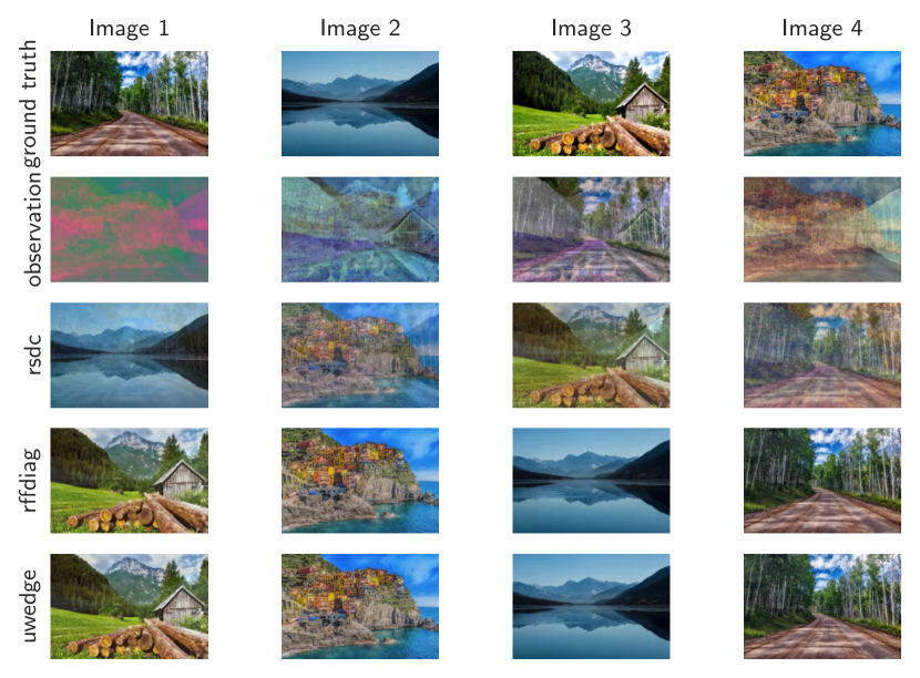
Figure 1: Results for image separation example from Section 6.3. The first row shows the original images, the second row the mixed images, and the last 3 rows show the unmixed images obtained by RSDC, RFFDIAG, and UWEDGE.

Table 5: Average running time in image separation

Algorithm name	Avg running time(ms)
RSDC	$2.32$
RFFDIAG	$23.39$
UWEDGE	$46.14$

6.4 Real data: electroencephalographic recordings

Finally, we test our randomized SDC algorithms on real electroencephalographic (EEG) recordings. In Human EEG, the signals observed at the different electrodes on the scalp are approximately linear mixtures of the source signals in the brain [19, Chapter 8.2]. Specifically, in [10] it is suggested that the eye-blinking noise signal can be separated by performing SDC on the Fourier cospectra of the EEG recording. This leads to a family of $d=33$ matrices of size $17\times 17$. We follow the implementation in [9], where the involved SDC solver is PHAM. The power spectrum and the topographic map of the estimated blink source signal with this default choice are shown in Figure 2. We can see that, from the topographic map of the source signal on the scalp, the source signal is indeed concentrated among the eyes, which confirms that this signal corresponds to eye-blink.

We applied RSDC and RFFDIAG to the same data and the results are shown in Figures 3 and 4 respectively. From the figures, we can see that both the algorithms identify the blink signals successfully and their power spectra are also close to the one estimated by the default solver. However, we can observe from the topographic map that the result of RSDC is more noisy.

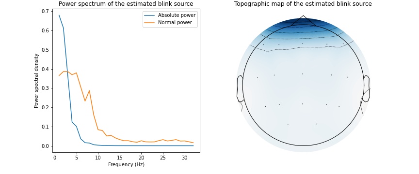
Figure 2: Power spectrum and topographic map of the blink source by PHAM

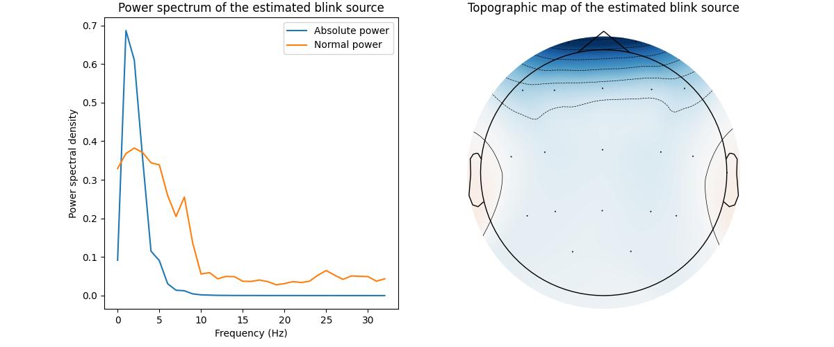
Figure 3: Power spectrum and topographic map of the blink source by RSDC

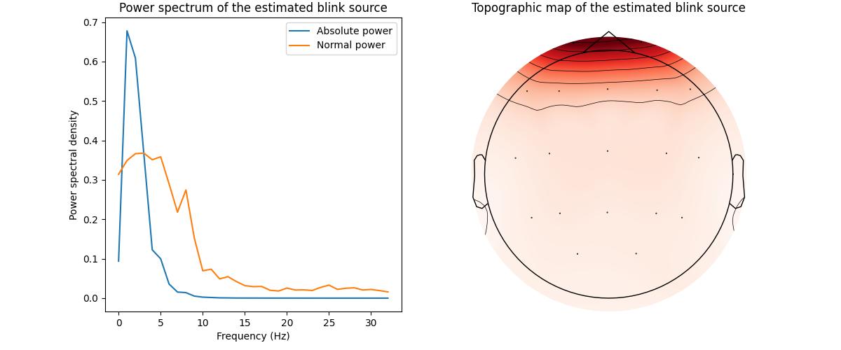
Figure 4: Power spectrum and topographic map of the blink source by RFFDIAG

Next, we compare the execution time of different SDC algorithms involved in this BSS task, averaged over $100$ repeated runs; see Table 6. In particular, RFFDIAG yields significantly faster performance than PHAM, while achieving a comparable level of accuracy.

Table 6: Average running time in eye-blind signal separation

Algorithm name	Avg running time(ms)
PHAM	$275.49$
RSDC	$1.42$
RFFDIAG	$2.69$

7 Conclusions

In this paper, we have proposed and analyzed RSDC, a novel randomized algorithm for performing (approximate) simultaneous diagonalization by congruence. Our numerical experiments show that this algorithm is best used in combination with an optimization method that uses the output of RSDC as starting point. The resulting algorithm, RFFDIAG, appears to offer a good compromise between efficiency and accuracy, outperforming existing solvers; sometimes by a large margin.

Acknowledgments.

The authors thank Nela Bosner, University of Zagreb, for inspiring discussions related to this work.

References

• Ablin et al. [2019] P. Ablin, J.-F. Cardoso, and A. Gramfort. Beyond Pham’s algorithm for joint diagonalization. In Proceedings of ESANN, Bruges, Belgium, April 2019.
• Absil and Gallivan [2006] P.-A. Absil and K. A. Gallivan. Joint diagonalization on the oblique manifold for independent component analysis. In Proceedings of ICASSP, volume V, pages 945–948, 2006.
• Absil et al. [2008] P.-A. Absil, R. Mahony, and R. Sepulchre. Optimization Algorithms on Matrix Manifolds. Princeton University Press, Princeton, NJ, 2008.
• Afsari [2008] B. Afsari. Sensitivity analysis for the problem of matrix joint diagonalization. SIAM J. Matrix Anal. Appl., 30(3), 2008.
• Anandkumar et al. [2012] A. Anandkumar, D. Hsu, and S. M. Kakade. A method of moments for mixture models and hidden markov models. In Proceedings of COLT, volume 23 of Proc. Mach. Learn. Res., pages 33.1–33.34, 2012.
• Anandkumar et al. [2014] A. Anandkumar, R. Ge, D. Hsu, S. M. Kakade, and M. Telgarsky. Tensor decompositions for learning latent variable models. J. Mach. Learn. Res., 15:2773–2832, 2014.
• Anandkumar et al. [2015] A. Anandkumar, D. P. Foster, D. Hsu, S. M. Kakade, and Y.-K. Liu. A spectral algorithm for latent Dirichlet allocation. Algorithmica, 72(1):193–214, 2015.
• Anderson et al. [1999] E. Anderson, Z. Bai, C. Bischof, L. S. Blackford, J. Demmel, J. Dongarra, J. Du Croz, A. Greenbaum, S. Hammarling, A. McKenney, and D. Sorensen. LAPACK Users’ Guide. Society for Industrial and Applied Mathematics, third edition, 1999.
• Barachant et al. [2022] A. Barachant, Q. Barthélemy, J.-R. King, A. Gramfort, S. Chevallier, P. L. C. Rodrigues, E. Olivetti, V. Goncharenko, G. W. vom Berg, G. Reguig, A. Lebeurrier, E. Bjäreholt, M. S. Yamamoto, P. Clisson, and M.-C. Corsi. pyriemann/pyriemann: v0.3, July 2022. URL https://pyriemann.readthedocs.io/en/latest/.
• Barthélemy et al. [2017] Q. Barthélemy, L. Mayaud, Y. Renard, D. Kim, S.-W. Kang, J. Gunkelman, and M. Congedo. Online denoising of eye-blinks in electroencephalography. Neurophysiol Clin., 47(5):371–391, 2017.
• Belouchrani et al. [1997] A. Belouchrani, K. Abed-Meraim, J.-F. Cardoso, and E. Moulines. A blind source separation technique using second-order statistics. IEEE Trans. Signal Process., 45(2):434–444, 1997.
• Bosner [2023] N. Bosner. Efficient algorithms for joint approximate diagonalization of multiple matrices. Preprint, 2023. URL https://doi.org/10.21203/rs.3.rs-2581723/v1.
• Bouchard et al. [2018] F. Bouchard, J. Malick, and M. Congedo. Riemannian optimization and approximate joint diagonalization for blind source separation. IEEE Trans. Signal Process., 66(8):2041–2054, 2018.
• Bouchard et al. [2020] F. Bouchard, B. Afsari, J. Malick, and M. Congedo. Approximate joint diagonalization with Riemannian optimization on the general linear group. SIAM J. Matrix Anal. Appl., 41(1):152–170, 2020.
• Boumal [2023] N. Boumal. An introduction to optimization on smooth manifolds. Cambridge University Press, 2023.
• Bustamante et al. [2020] M. D. Bustamante, P. Mellon, and M. V. Velasco. Solving the problem of simultaneous diagonalization of complex symmetric matrices via congruence. SIAM J. Matrix Anal. Appl., 41(4):1616–1629, 2020.
• Cardoso [1994] J.-F. Cardoso. On the performance of orthogonal source separation algorithms. In Proceedings of EUSIPCO, volume 94, pages 776–779, 1994.
• Chabriel et al. [2014] G. Chabriel, M. Kleinsteuber, E. Moreau, H. Shen, P. Tichavský, and A. Yeredor. Joint matrices decompositions and blind source separation: A survey of methods, identification, and applications. IEEE Signal Process. Mag., 31(3):34–43, 2014.
• Congedo et al. [2014] M. Congedo, S. Rousseau, and C. Jutten. An introduction to eeg source analysis with an illustration of a study on error-related potentials. In Guide to Brain-Computer Music Interfacing, pages 163–189. Springer, 2014.
• Corless et al. [1997] R. M. Corless, P. M. Gianni, and B. M. Trager. A reordered Schur factorization method for zero-dimensional polynomial systems with multiple roots. In Proceedings of ISSAC, pages 133–140. ACM, 1997.
• De Lathauwer [2006] L. De Lathauwer. A link between the canonical decomposition in multilinear algebra and simultaneous matrix diagonalization. SIAM J. Matrix Anal. Appl., 28(3):642–666, 2006.
• Dixon [1983] J. D. Dixon. Estimating extremal eigenvalues and condition numbers of matrices. SIAM J. Numer. Anal., 20(4):812–814, 1983.
• Ehler et al. [2019] M. Ehler, S. Kunis, T. Peter, and C. Richter. A randomized multivariate matrix pencil method for superresolution microscopy. Electron. Trans. Numer. Anal., 51:63–74, 2019.
• Evert et al. [2022a] E. Evert, M. Vandecappelle, and L. De Lathauwer. Canonical polyadic decomposition via the generalized Schur decomposition. IEEE Signal Process. Lett., 29:937–941, 2022a.
• Evert et al. [2022b] E. Evert, M. Vandecappelle, and L. De Lathauwer. A recursive eigenspace computation for the canonical polyadic decomposition. SIAM J. Matrix Anal. Appl., 43(1):274–300, 2022b.
• Golub and Van Loan [2013] G. H. Golub and C. F. Van Loan. Matrix computations. Johns Hopkins Studies in the Mathematical Sciences. JHU Press, Baltimore, MD, fourth edition, 2013.
• He and Kressner [2024] H. He and D. Kressner. Randomized joint diagonalization of symmetric matrices. SIAM J. Matrix Anal. Appl., 45(1):661–684, 2024.
• Jiang and Li [2016] R. Jiang and D. Li. Simultaneous diagonalization of matrices and its applications in quadratically constrained quadratic programming. SIAM J. Optim., 26(3):1649–1668, 2016.
• Khachatrian et al. [2021] E. Khachatrian, S. Chlaily, T. Eltoft, W. Dierking, F. Dinessen, and A. Marinoni. Automatic selection of relevant attributes for multi-sensor remote sensing analysis: A case study on sea ice classification. IEEE J. Sel. Top. Appl. Earth Obs. Remote Sens., 14:9025–9037, 2021.
• Kågström and Kressner [2006] B. Kågström and D. Kressner. Multishift variants of the QZ algorithm with aggressive early deflation. SIAM J. Matrix Anal. Appl., 29(1):199–227, 2006.
• Kressner [2005] D. Kressner. Numerical methods for general and structured eigenvalue problems, volume 46 of Lecture Notes in Computational Science and Engineering. Springer-Verlag, Berlin, 2005.
• Le and Nguyen [2022] T. H. Le and T. N. Nguyen. Simultaneous diagonalization via congruence of Hermitian matrices: some equivalent conditions and a numerical solution. SIAM J. Matrix Anal. Appl., 43(2):882–911, 2022.
• Pfister et al. [2019] N. Pfister, S. Weichwald, P. Bühlmann, and B. Schölkopf. Robustifying independent component analysis by adjusting for group-wise stationary noise. J. Mach. Learn. Res., 20:Paper No. 147, 50, 2019.
• Pham [2001] D. T. Pham. Joint approximate diagonalization of positive definite Hermitian matrices. SIAM J. Matrix Anal. Appl., 22(4):1136–1152, 2001.
• Pham and Cardoso [2001] D. T. Pham and J.-F. Cardoso. Blind separation of instantaneous mixtures of nonstationary sources. IEEE Trans. Signal Process., 49(9):1837–1848, 2001.
• Steel [2023] T. Steel. Fast Algorithms for Generalized Eigenvalue Problems. PhD thesis, KU Leuven, 2023.
• Stewart and Sun [1990] G. W. Stewart and J.-G. Sun. Matrix perturbation theory. Computer Science and Scientific Computing. Academic Press, Inc., Boston, MA, 1990.
• Sun [1998. Revised 2002] J.-G. Sun. Stability and accuracy: Perturbation analysis of algebraic eigenproblems. Technical Report UMINF 98-07, Department of Computing Science, University of Umeå, Umeå, Sweden, 1998. Revised 2002. Available from https://people.cs.umu.se/jisun/Jiguang-Sun-UMINF98-07-rev2002-02-20.pdf.
• Sutton [2023] B. Sutton. Simultaneous diagonalization of nearly commuting Hermitian matrices: do-one-then-do-the-other. IMA J. Numer. Anal, page drad033, 2023.
• Tichavský and Yeredor [2009] P. Tichavský and A. Yeredor. Fast approximate joint diagonalization incorporating weight matrices. IEEE Trans. Signal Process., 57(3):878–891, 2009.
• Urdaneta and Leon [2018] H. L. Urdaneta and H. F. O. Leon. Solving joint diagonalization problems via a Riemannian conjugate gradient method in Stiefel manifold. Proc. Ser. Brazil. Soc. Comput. Appl. Math, 6(2), 2018.
• Zhang et al. [2022] S. Zhang, E. Soubies, and C. Févotte. Leveraging joint-diagonalization in transform-learning NMF. IEEE Trans. Signal Process., 70:3802–3817, 2022.
• Ziehe et al. [2003/04] A. Ziehe, P. Laskov, G. Nolte, and K.-R. Müller. A fast algorithm for joint diagonalization with non-orthogonal transformations and its application to blind source separation. J. Mach. Learn. Res., 5:777–800, 2003/04.