Event-Triggered Parameterized Control of Nonlinear Systems

Abstract

This paper deals with event-triggered parameterized control (ETPC) of nonlinear systems with external disturbances. In this control method, between two successive events, each control input to the plant is a linear combination of a set of linearly independent scalar functions. At each event, the controller updates the coefficients of the parameterized control input so as to minimize the error in approximating a continuous time control signal and communicates the same to the actuator. We design an event-triggering rule that guarantees global uniform ultimate boundedness of trajectories of the closed loop system. We also ensure the absence of zeno behavior by showing the existence of a uniform positive lower bound on the inter-event times. We illustrate our results through numerical examples, which indicate that the proposed control method leads to a significant improvement in average inter-event time and minimum inter-event time compared to the event-triggered zero-order-hold control.

I INTRODUCTION

Event-triggered control (ETC) is a commonly used control method in applications with resource constraints. Most of the ETC literature designs zero-order-hold (ZOH) sampled-data controllers. However, in many common communication protocols, including TCP and UDP [1], there is a minimum packet size. Thus, ZOH control may lead to an increase in the total number of communication instances due to under utilization of each packet. With this motivation, in this paper, we propose a non-ZOH control method and design it for control of nonlinear systems with external disturbances.

I-A Literature Review

An introduction to ETC and an overview of the literature on it can be found in [2, 3, 4, 5]. Typically, in ETC and in the closely related self-triggered control [6] and periodic event-triggered control [7], control input is applied in ZOH fashion, i.e., the control input to the plant is held constant between any two successive events. There are some exceptions to this rule though. For example, in model-based ETC [8, 9, 10, 11, 12], both the controller and the actuator use identical copies of a model of the system, whose states are updated synchronously in an event-triggered manner. The model generates a time-varying control input even between two successive events. In event/self-triggered model predictive control [13, 14, 15], the actuator applies a part of an optimal control trajectory, which is generated by solving a finite horizon optimal control problem at each triggering instant. Recent studies in [16, 17] show that communication resources can be utilized more efficiently by transmitting only some of the samples of the generated control trajectory to the actuator, based on which a sampled data first-order-hold (FOH) control input is applied. In event-triggered dead-beat control [18], a sequence of control inputs is transmitted to the actuator in an event-triggered manner. The actuator stores this control sequence in a buffer and applies it till the next packet is received. In team-triggered control [19, 20] each agent makes promises to its neighbors about their future states or controls and informs them if these promises are violated later.

References [21, 22, 23] use generalized sampled-data hold functions (GSHF) in the control of linear time-invariant systems. The idea of GSHF is to periodically sample the output of the system and generate the control by means of a hold function applied to the resulting sequence. To the best of our knowledge, this idea was first explored in the context of ETC only in our recent work [24], in which we propose an event-triggered parameterized control (ETPC) method for stabilization of linear systems. In [25], we use a similar idea to design an event-triggered polynomial controller for trajectory tracking by unicycle robots.

I-B Contributions

The contributions of this paper are given below:

• We design an event-triggered parameterized controller, for nonlinear systems with external disturbances, that guarantees global uniform ultimate boundedness of trajectories of the closed loop system and non-Zeno behavior of inter-event times.

• Our approach requires fewer communication packets compared to ZOH or FOH control, as our method can be fine tuned to utilize the full payload of each packet.

• Compared to model-based ETC, our method requires lesser computational resources at the actuator and also provides greater privacy and security.

• Compared to model-based ETC and GSHF based control, we can easily generalize our approach to a variety of settings, including to nonlinear systems and distributed systems.

• Compared to the event-triggered MPC or deadbeat control method, at each event, our proposed method requires only a limited number of parameters to be sent irrespective of the time duration of the signal.

• In this paper, we generalize the control method proposed in our previous work [24] to nonlinear control settings with external disturbances. Our recent work [25] considers a similar control method for the trajectory tracking by unicycle robots using event-triggered polynomial control. On the other hand, in the current paper, we consider a more generalized problem setup and also incorporate the effect of external disturbances.

I-C Notation

Let , $\mathbb{R}_{\geq 0}$ and $\mathbb{R}_{>0}$ denote the set of all real numbers, the set of non-negative real numbers and the set of positive real numbers, respectively. Let ${\mathbb{N}}$ and ${\mathbb{N}}_{0}$ denote the set of all positive and non-negative integers, respectively. For any $x\in^{n}$, $\left\lVert x\right\rVert$ denotes the euclidean norm. A continuous function $\alpha:[0,\infty)\to[0,\infty)$ is said to be of class $\mathcal{K}_{\infty}$ if it is strictly increasing, $\alpha(0)=0$ and $\alpha(r)\to\infty$ as $r\to\infty$. For any right continuous function $f:_{\geq 0}\to^{n}$ and $t\geq 0$, $f(t^{+}):=\lim\limits_{s\to t^{+}}f(s)$. For any two functions $v,w:[0,\infty]\rightarrow_{\geq 0}$ and $y\in\mathbb{R}_{>0}$, let

$$\langle v,w\rangle_{y}^{T}:=\int_{0}^{T}y^{\tau}v(\tau)w(\tau)\mathrm{d}\tau.$$

Note that $\langle v,w\rangle_{y}^{T}$ is the inner product of the functions $y^{\tau/2}v(\tau)$ and $y^{\tau/2}w(\tau)$ restricted to the domain of $\tau$ to $[0,T]$.

II PROBLEM SETUP

In this section, we present the system dynamics, the parameterized control law and the objective of this paper.

System Dynamics and Control Law

Consider a nonlinear system with external disturbance,

$$\dot{x}=f(x,u,d),\quad\forall t\geq t_{0}=0,$$ (1)

where $x\in^{n}$, $u\in^{m}$, $d\in^{q}$ and $t\in\mathbb{R}_{\geq 0}$, respectively, denote the system state, the control input, the external disturbance and the time. In this paper, we consider event-triggered generalized sampled data control instead of the typical zero-order hold control. We call our proposed method event-triggered parametrized control (ETPC).

Specifically, consider a set of functions

$$\Phi:=\left\{\phi_{j}:[0,\infty]\to\right\}_{j=0}^{p}.$$

We let the $i^{\text{th}}$ control input, for $i\in\{1,2,\ldots,m\}$, between two successive events be

$$u_{i}(t_{k}+\tau)=P(\textbf{a}_{i}(k),\tau):=\sum_{j=0}^{p}a_{ji}(k)\phi_{j}(\tau),\ \forall\tau\in[0,t_{k+1}-t_{k}).$$

Here $(t_{k})_{k\in{\mathbb{N}}_{0}}$ is the sequence of communication time instants at which the controller updates the coefficients of the parameterized control input, $\textbf{a}(k):=[a_{ji}(k)]\in^{(p+1)\times m}$, and communicates them to the actuator. The update times $(t_{k})_{k\in{\mathbb{N}}_{0}}$ are determined in an event-triggered manner. Now, we can write the control law as,

$$u(t_{k}+\tau)=\textbf{a}^{\text{T}}(k)\phi(\tau),\ \forall\tau\in[0,t_{k+1}-t_{k}),$$ (2)

where $\phi(\tau):=\begin{bmatrix}\phi_{0}(\tau)&\phi_{1}(\tau)&\ldots&\phi_{p}(\tau)\end{bmatrix}^{\text{T}}$.

The general configuration of the ETPC system considered in this paper is depicted in Figure 1.

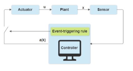
Figure 1: Event-triggered parameterized control configuration

Here, the system state is continuously available to the controller which has enough computational resources to evaluate the event-triggering condition and to update the coefficients of the control input at an event-triggering instant.

Assumptions

We make the following assumptions throughout this paper.

1. There exist $\gamma:^{n}\to^{m}$ and a continuously differentiable Lyapunov-like function $V:^{n}\to$ such that

   $$\alpha_{1}(\left\lVert x\right\rVert)\leq V(x)\leq\alpha_{2}(\left\lVert x\right\rVert),$$

   $$\frac{\partial V}{\partial x}f(x,\gamma(x)+e,d)\leq-\alpha_{3}(\left\lVert x\right\rVert)+\rho_{1}(\left\lVert e\right\rVert)+\rho_{2}(\left\lVert d\right\rVert)$$

   where $\alpha_{1}(.)$, $\alpha_{2}(.)$, $\alpha_{3}(.)$, $\rho_{1}(.)$, $\rho_{2}(.)$ are class $\mathcal{K}_{\infty}$ functions and $e\in^{m}$ is the actuation error.

2. $f(.)$ is Lipschitz on compact sets, with $f(0)=0$ and $\gamma(.)$ is continuously differentiable with $\gamma(0)=0$.

3. There exists $D\geq 0$ such that $\left\lVert d(t)\right\rVert\leq D,\ \forall t\geq t_{0}$.

Note that, Assumption (A1) indicates that there exists a continuous-time feedback controller that makes the system (1) input-to-state-stable (ISS) with respect to the actuation error $e$ and the external disturbance $d$. Assumption (A2) is a common technical assumption in the literature on nonlinear systems. Finally, Assumption (A3) means that the disturbance signal is uniformly upper bounded, which is again common in the literature. Throughout this paper, we make the following standing assumption regarding $\Phi$.

1. Each function $\phi_{j}\in\Phi$ is continuously differentiable. $\phi_{0}$ is a non-zero constant function and $\phi_{j}(0)=0$, $\forall j\in\{1,2,\ldots,p\}$. Let $T$ be a fixed parameter and suppose $\Phi$ is a set of linearly independent functions when restricted to $[0,T]$, i.e., $\sum_{j=0}^{p}c_{j}\phi_{j}(t)=0,$ $\forall t\in[0,T]$ iff $c_{j}=0,$ $\forall j\in\{0,1,\ldots,p\}$.

Objective

Our objective is to design a parameterized control law (2) and an event-triggering rule for implicitly determining the communication instants $(t_{k})_{k\in{\mathbb{N}}_{0}}$ so that the trajectories of the closed loop system are globally uniformly ultimately bounded. We also wish to ensure the absence of zeno behavior by showing the existence of a uniform positive lower bound on the inter-event times.

III DESIGN AND ANALYSIS OF EVENT-TRIGGERED CONTROLLER

In this section, we first design a parameterized control law and an event-triggering rule to achieve our objective. Then, we analyze the designed control system.

III-A Control Law

The proposed control method is based on the idea of emulating a continuous time model based control signal using a parametrized time-varying signal as in (2). In particular, consider the following model for some time horizon $T$,

$$\dot{\hat{x}}=f(\hat{x},\gamma(\hat{x}),0),\quad\forall t\in[t_{k},t_{k}+T],\quad\hat{x}(t_{k})=x(t_{k}),\ k\in{\mathbb{N}}_{0}.$$ (3)

Here $\hat{x}$ is the state of the model, which is the same as (1) but with zero disturbance. The model state is reinitialized with $\hat{x}(t_{k})=x(t_{k})$ at each event time $t_{k}$ for $k\in{\mathbb{N}}_{0}$. Now consider the open-loop control signals

$$\hat{u}_{i}(\tau):=\gamma_{i}(\hat{x}(t_{k}+\tau)),\quad\forall i\in\{1,2,\ldots,m\},$$

where $\gamma_{i}(\hat{x}(t_{k}+\tau))$ is the $i^{th}$ component of $\gamma(\hat{x}(t_{k}+\tau))$. One way to potentially reduce the number of communication instances is to transmit the whole control signal $\hat{u}(\tau)$ for $\tau\in[0,T]$. For example, this is what is done in event-triggered deadbeat control [18] and MPC [13, 14]. However, transmitting the whole control signal $\gamma(\hat{x}(t_{k}+\tau))$ for $\tau\in[0,T)$ in a communication packet at $t_{k}$ may be too costly.

So, in our proposed idea, we approximate $\hat{u}_{i}(\tau)$ for each $i$ in the linear span of $\Phi$. Specifically, we solve the following finite horizon optimization problem to determine the coefficients of the parameterized control signal (2) that is to be applied starting at $t_{k}$. For $i\in\{1,2,\ldots,m\}$,

$$\textbf{a}_{i}(k)\in\operatorname*{arg\,min}_{a\in^{p+1}} \int_{0}^{T}\delta^{\tau}|P(a,\tau)-\hat{u}_{i}(\tau)|^{2}d\tau,$$ (4)

s.t. $$|P(a,0)-\hat{u}_{i}(0)|\leq\eta(\left\lVert\hat{x}(t_{k})\right\rVert)$$

for a function $\eta:_{\geq 0}\to_{\geq 0}$ with $\eta(0)=0$ and for a finite time horizon $T>0$. The function $\eta$ and the time horizon $T$ are to be designed. Here, $\delta\in(0,1)$ is a discounting factor that prioritises the approximation error in the short-term compared to the long-term, while solving the optimization problem (4). Note that, we require the signal $\hat{u}(\tau)$ for $\tau\in[0,T]$ to solve the optimization problem (4). This signal can be obtained by numerically simulating the $\hat{x}$ dynamics (3).

Remark 1.

(Control input for $\tau>T$). With the parameters $\textbf{a}(k)$ obtained by solving (4), the control input applied by the actuator is as given in (2). Since $t_{k}$’s are implicitly determined by an event-triggering rule online, it may happen that $t_{k+1}-t_{k}>T$. However, even though we find $\textbf{a}(k)$ by using $\hat{u}(\tau)$ for $\tau\in[0,T]$, $P(\textbf{a}_{i},\tau)$, for each $i$, is well defined $\forall\tau\in[0,\infty]$. Hence, control input $u(t_{k}+\tau)$ for $\tau$ is well defined for entire interval $[t_{k},t_{k+1})$ even if $t_{k+1}-t_{k}>T$. $\bullet$

Note that, we can rewrite the optimization problem (4) as,

$$\min_{a\in^{p+1}}J_{i}(a),\quad\textrm{s.t. }\ F_{i}(a)\leq 0,$$ (5)

where,

$$J_{i}(a)=\langle\hat{u}_{i},\hat{u}_{i}\rangle_{\delta}^{T}-2\sum_{j=0}^{p}a_{j}\langle\hat{u}_{i},\phi_{j}\rangle_{\delta}^{T}+\sum_{j=0}^{p}\sum_{l=0}^{p}a_{j}a_{l}\langle\phi_{j},\phi_{l}\rangle_{\delta}^{T},$$

$$F_{i}(a)=\begin{bmatrix}a_{0}\phi_{0}(0)-\hat{u}_{i}(0)-\eta(\left\lVert\hat{x}(t_{k})\right\rVert)\\ -a_{0}\phi_{0}(0)+\hat{u}_{i}(0)-\eta(\left\lVert\hat{x}(t_{k})\right\rVert)\end{bmatrix}.$$

Proposition 2.

Problem (5) is a strictly convex optimization problem and it is always feasible.

Proof.

Let us first show that the cost function of (5), $J_{i}(a)$, is strictly convex in the optimization variables $a$. The Hessian matrix of $J_{i}(.)$ for all $i\in\{1,2,\ldots,m\}$, denoted as H, is

$$\textbf{H}=2\begin{bmatrix}\langle\phi_{0},\phi_{0}\rangle_{\delta}^{T}&\langle\phi_{0},\phi_{1}\rangle_{\delta}^{T}&\ldots&\langle\phi_{0},\phi_{p}\rangle_{\delta}^{T}\\[5.0pt] \langle\phi_{1},\phi_{0}\rangle_{\delta}^{T}&\langle\phi_{1},\phi_{1}\rangle_{\delta}^{T}&\ldots&\langle\phi_{1},\phi_{p}\rangle_{\delta}^{T}\\ \ldots&\ldots&\ldots&\ldots\\ \langle\phi_{p},\phi_{0}\rangle_{\delta}^{T}&\langle\phi_{p},\phi_{1}\rangle_{\delta}^{T}&\ldots&\langle\phi_{p},\phi_{p}\rangle_{\delta}^{T}\end{bmatrix}.$$ (6)

Observe that H is twice the Gram matrix for the functions in $\bar{\Phi}:=\{\bar{\phi}_{j}:[0,T]\to\}_{j=0}^{p}$ where $\bar{\phi}_{j}(\tau):=\delta^{\frac{\tau}{2}}\phi_{j}(\tau)$. Additionally, $\bar{\Phi}$ is a set of linearly independent functions as $\Phi$ is a set of linearly independent functions when restricted to $[0,T]$ and as $\delta\in(0,1)$. Thus, we can say that H is a positive definite matrix. Hence, the cost function in (5) is strictly convex. Note that the only constraints in the optimization problem (5) are two linear inequality constraints in $a_{0}$, the coefficient of the constant function in $\Phi$. Thus, (5) is a strictly convex optimization problem. Problem (5) is always feasible as the choice $a_{0}\phi_{0}(0)=\hat{u}_{i}(0)$ and $a_{i}=0$ for $i\in\{1,\ldots,p\}$, which is the zero order hold signal, satisfies the constraints. ∎

Proposition 2 implies that Problem (5) always has exactly one optimal solution.

III-B Event-Triggering Rule

We consider the following event-triggering rule.

$$t_{k+1}=\min\{t>t_{k}\ :\rho_{1}(\left\lVert e\right\rVert)\geq\frac{\sigma}{2}\alpha_{3}(\left\lVert x\right\rVert)\text{ and }V(x)\geq\epsilon\},$$ (7)

where $e:=u-\gamma(x)$, $\epsilon:=\alpha_{2}(\alpha_{3}^{-1}(\frac{2\rho_{2}(D)}{\sigma}))\geq 0$ and $\sigma\in(0,1)$ is a design parameter. Here $\rho_{1}(.)$, $\rho_{2}(.)$, $\alpha_{2}(.)$, and $\alpha_{3}(.)$ are the same class $\mathcal{K}_{\infty}$ functions given in Assumption (A1). Note that, here, $e$ denotes the error between the actual control input $u$ and the “ideal” feedback control input $\gamma(x)$. This error is different from the approximation error $u-\hat{u}$ as the dynamics of $x$ and $\hat{x}$ are different.

In summary, the closed loop system, $\mathscr{S}$, is the combination of the system dynamics (1), the control law (2), with coefficients chosen by solving (4), which are updated at the events determined by the event-triggering rule (7). That is,

$$\mathscr{S}:\ \eqref{eq:sys},\eqref{eq:control_law},\eqref{eq:a_ik},\eqref{eq:etr}.$$ (8)

Remark 3.

(Computational requirement of the controller). We suppose that the controller has enough computational resources to evaluate the event-triggering condition (7) and to solve the finite horizon optimization problem (5) at any triggering instant. Note that, event-triggered MPC or deadbeat control methods also have similar computational requirements at the controller. $\bullet$

III-C Analysis of the event-triggered control system

Next, we show that the trajectories of the closed loop system (8) are globally uniformly ultimately bounded and the inter-event times have a uniform positive lower bound that depends on the initial state of the system. First, let

$$\epsilon_{k}:=V(x(t_{k})),\ k\in{\mathbb{N}}_{0},\quad\bar{\epsilon}:=\max\{\epsilon,\epsilon_{0}\}.$$

Following lemma helps to prove the main result of this paper.

Lemma 4.

Consider system (8) and let Assumptions (A1) - (A4) hold. Let $\eta(.):=\frac{1}{\sqrt{m}}\rho_{1}^{-1}(r\frac{\sigma}{2}\alpha_{3}(.))$ with $r\in[0,1)$. Then, $V(x(t))\leq\epsilon_{k}\leq\bar{\epsilon},\forall t\in[t_{k},t_{k+1})$ and $\forall k\in{\mathbb{N}}$.

Proof.

Let us first calculate the time derivative of $V(.)$ along the trajectories of system (8) as follows,

$$\dot{V} =\frac{\partial V}{\partial x}f(x,u,d)=\frac{\partial V}{\partial x}f(x,\gamma(x)+e,d),$$

$$\leq-\alpha_{3}(\left\lVert x\right\rVert)+\rho_{1}(\left\lVert e\right\rVert)+\rho_{2}(\left\lVert D\right\rVert),$$

$$\leq-(1-\sigma)\alpha_{3}(\left\lVert x\right\rVert)-\left(\frac{\sigma}{2}\alpha_{3}(\left\lVert x\right\rVert)-\rho_{1}(\left\lVert e\right\rVert)\right),\forall V(x)\geq\epsilon.$$

The first inequality follows from Assumptions (A1) and (A3). The last inequality follows from the fact that $V(x)\geq\epsilon$ implies $\left\lVert x\right\rVert\geq\alpha_{2}^{-1}(\epsilon)=\alpha_{3}^{-1}\left(\frac{2\rho_{2}(D)}{\sigma}\right)$. Note that according to the inequality constraint in (4), $\left\lVert e(t_{k}^{+})\right\rVert\leq\sqrt{m}\eta(\left\lVert x(t_{k}^{+})\right\rVert),\ \forall k\in{\mathbb{N}}_{0}$. From the definition of $\eta(.)$ and the fact that $r\in[0,1)$, we see that $\rho_{1}(\left\lVert e(t_{k}^{+})\right\rVert)<\frac{\sigma}{2}\alpha_{3}(\left\lVert x(t_{k}^{+})\right\rVert),\ \forall k\in{\mathbb{N}}_{0}$. Further, the event-triggering rule (7) implies that $V(x(t_{k}^{+}))=\epsilon_{k}\geq\epsilon,\ \forall k\in{\mathbb{N}}$ and hence $\dot{V}(x(t_{k}^{+}))\leq-(1-\sigma)\alpha_{3}(\left\lVert x(t_{k}^{+})\right\rVert)<0,\ \forall k\in{\mathbb{N}}$.

Now, let us prove the statement that $V(x(t))\leq\epsilon_{k},\ \forall t\in[t_{k},t_{k+1})$ and $\forall k\in{\mathbb{N}}$ by contradiction. Suppose that this statement is not true. Then, as $V(x(t))$ is a continuous function of time, there must exist $\bar{t}\in(t_{k},t_{k+1})$, for some $k\in{\mathbb{N}}$, such that $V(x(\bar{t}))=\epsilon_{k}$ and $\dot{V}(x(\bar{t}))>0$. However, since $\epsilon_{k}\geq\epsilon$ and the event-triggering condition is not satisfied at $t=\bar{t}$, $\rho_{1}(\left\lVert e(\bar{t})\right\rVert)<\frac{\sigma}{2}\alpha_{3}(\left\lVert x(\bar{t})\right\rVert)$, which means that $\dot{V}(x(\bar{t}))\leq-(1-\sigma)\alpha_{3}(\left\lVert x(\bar{t})\right\rVert)<0$. As there is a contradiction, we conclude that there does not exist such a $\bar{t}$ and hence $V(x(t))\leq\epsilon_{k},\ \forall t\in[t_{k},t_{k+1})$ and $\forall k\in{\mathbb{N}}$.

Next, note that if $\epsilon_{0}\leq\epsilon$ then according to the event-triggering rule (7), $\epsilon_{1}=\epsilon=\bar{\epsilon}$. If $\epsilon_{0}>\epsilon$ then following similar arguments as before we can show that $V(x(t))\leq\epsilon_{0},\ \forall t\in[t_{0},t_{1})$ and hence $\epsilon_{1}\leq\epsilon_{0}=\bar{\epsilon}$. Thus, the claim that $\epsilon_{k}\leq\bar{\epsilon}$ for all $k\in{\mathbb{N}}$ follows by induction. ∎

Note that Lemma 4 does not impose any restrictions on $x(t_{0})$. In particular, it is possible that $V(x(t_{0}))<\epsilon$. Lemma 4 only makes a claim about $V(x(t))$ for $t\in[t_{k},t_{k+1})$ and for any $k\in{\mathbb{N}}$. Now, we present the main result of this paper.

Theorem 5.

(Absence of Zeno behavior and global uniform ultimate boundedness). Consider system (8) and let Assumptions (A1) - (A4) hold. Let $\eta(.):=\frac{1}{\sqrt{m}}\rho_{1}^{-1}(r\frac{\sigma}{2}\alpha_{3}(.))$.

• If $\alpha_{3}^{-1}(.)$ and $\rho_{1}(.)$ are lipschitz on compact sets and if $r\in\left[0,\frac{\alpha_{3}(\alpha_{2}^{-1}(\epsilon)}{\alpha_{3}(\alpha_{1}^{-1}(\bar{\epsilon}))}\right)$, then the inter-event times, $t_{k+1}-t_{k},\ \forall k\in{\mathbb{N}}$, are uniformly lower bounded by a positive number that depends on the initial state of the system.

• The trajectories of the closed loop system are globally uniformly ultimately bounded with global uniform ultimate bound $\alpha_{1}^{-1}(\epsilon)$.

Proof.

Let us prove the first statement of this theorem. First, note that Assumption (A1) implies $\alpha_{1}(\left\lVert x\right\rVert)\leq\alpha_{2}(\left\lVert x\right\rVert)$ $\forall x\in^{n}$ and then by the definition of $\bar{\epsilon}$, we can say that $r\in[0,1)$. Now, we consider the compact set $R:=\{x\in^{n}:V(x)\leq\bar{\epsilon}\}$. Lemma 4 implies that $x(t)\in R,\ \forall t\in[t_{k},t_{k+1}),\forall k\in{\mathbb{N}}$. Note that according to the proof of Lemma 4, $\left\lVert e(t_{k}^{+})\right\rVert\leq\rho_{1}^{-1}(r\frac{\sigma}{2}\alpha_{3}(\left\lVert x(t_{k}^{+})\right\rVert)),\ \forall k\in{\mathbb{N}}_{0}$. Now, by using the fact that $\alpha_{2}^{-1}(\epsilon)\leq\left\lVert x(t_{k})\right\rVert\leq\alpha_{1}^{-1}(\bar{\epsilon}),\forall k\in{\mathbb{N}}$, we can say that the inter-event time must at least be equal to the time it takes $\left\lVert e\right\rVert$ to grow from $e_{1}:=\rho_{1}^{-1}(r\frac{\sigma}{2}\alpha_{3}(\alpha_{1}^{-1}(\bar{\epsilon})))$ to $e_{2}:=\rho_{1}^{-1}(\frac{\sigma}{2}\alpha_{3}(\alpha_{2}^{-1}(\epsilon)))$. Note that, if $r$ is chosen as in the statement of the result, then we can guarantee that $e_{1}<e_{2}$. Next, we present a claim.
Claim (a): There exist $\beta_{1},\beta_{2}>0$ such that $\left\lVert u(t)\right\rVert\leq\beta_{1}$ and $\left\lVert\dot{u}(t)\right\rVert\leq\beta_{2}$, $\forall t\in[t_{k},\min\{t_{k+1},t_{k}+T\})$, $\forall k\in{\mathbb{N}}_{0}$.

Let us prove claim (a). Recall that, $\forall i\in\{1,2,\ldots,m\}$ and $\forall k\in{\mathbb{N}}_{0}$, $u_{i}(t)$ for $t\in[t_{k},t_{k+1})$ is chosen by solving the problem (4), which is equivalent to (5). Now, we can write the corresponding Lagrangian as $\mathscr{L}_{i}(a,\mu)=J_{i}(a)+\mu_{i}^{\text{T}}F_{i}(a)$, where $\mu_{i}\in^{2}$ is the Lagrange multiplier. Recall from Proposition 2 that the optimization problem (5) is strictly convex with two linear inequality constraints. So, strong duality holds for problem (5) and any optimal primal-dual solution $(\textbf{a}_{i}(k),\mu_{i}(k))$ must satisfy the Karush-Kuhn-Tucker (KKT) conditions. The stationarity conditions can be represented in matrix form as follows,

$$\textbf{H}\textbf{a}_{i}(k)=D_{i}(k)$$

where H is the Hessian matrix given in (6) and

$$D_{i}(k)=2\begin{bmatrix}\langle\hat{u}_{i},\phi_{0}\rangle_{\delta}^{T}\\[3.00003pt] \langle\hat{u}_{i},\phi_{1}\rangle_{\delta}^{T}\\ \vdots\\ \langle\hat{u}_{i},\phi_{p}\rangle_{\delta}^{T}\end{bmatrix}-\begin{bmatrix}\phi_{0}(0)&-\phi_{0}(0)\\ 0&0\\ \vdots&\vdots\\ 0&0\end{bmatrix}\mu_{i}(k).$$

Further, the complementary slackness conditions are

$$\mu_{i1}(k)(\textbf{a}_{i0}(k)\phi_{0}(0)-\hat{u}_{i}(0)-\eta(\left\lVert x(t_{k})\right\rVert)) =0$$

$$\mu_{i2}(k)(-\textbf{a}_{i0}(k)\phi_{0}(0)+\hat{u}_{i}(0)-\eta(\left\lVert x(t_{k})\right\rVert)) =0.$$

Recall that, H is a positive definite matrix and hence it is invertible. So, every optimal primal-dual solution $(\textbf{a}_{i}(k),\mu_{i}(k))$ to problem (5) must satisfy $\textbf{a}_{i}(k)=\textbf{H}^{-1}D_{i}(k)$. Note that, for any $k\in{\mathbb{N}}_{0}$, $\hat{x}(t_{k})=x(t_{k})\in R$, which implies that $\hat{x}(t)\in R$ for all $t\in[t_{k},t_{k}+T)$ as $\dot{V}(\hat{x})\leq-\alpha_{3}(\hat{x})\leq 0$. Now, note that,

$$|\hat{u}_{i}(\tau)|\leq\left\lVert\gamma(\hat{x}(t_{k}+\tau))\right\rVert\leq L_{\gamma},$$

for some $L_{\gamma}>0$, where the last inequality follows from the fact that $\gamma(.)$ is lipschitz on the compact set $R$ with $\gamma(0)=0$ and $\left\lVert\hat{x}\right\rVert\leq\alpha_{1}^{-1}(\bar{\epsilon})$ for all $\hat{x}\in R$. Thus, the norm of the first term in $D_{i}(k)$ is uniformly, $\forall k\in{\mathbb{N}}_{0}$, upper bounded by a constant, say $b\geq 0$. Let $h:=\left\lVert\textbf{H}^{-1}\right\rVert$. If for the optimal solution $\textbf{a}_{i}(k)$ to problem (5), the constraints are not active then $\mu_{i}(k)=0$ and we can see that $\left\lVert\textbf{a}_{i}(k)\right\rVert$ is upper bounded by $hb$. If on the other hand, $\mu_{i}(k)\neq 0$, then $\textbf{a}_{i0}(k)$ can be solved for from the complementary slackness conditions. Recall from Assumption (A2) that $\gamma$ is continuously differentiable, which guarantees that it is bounded on compact sets. Thus, the magnitude of $\textbf{a}_{i0}(k)$ is uniformly, $\forall k\in{\mathbb{N}}_{0}$, upper bounded by some constant as $\eta(\left\lVert x(t_{k})\right\rVert)$ and $\hat{u}_{i}(0)=\left\lVert\gamma_{i}(\hat{x}(t_{k}))\right\rVert$ are upper bounded for all $k\in{\mathbb{N}}_{0}$ since $\hat{x}(t_{k})=x(t_{k})\in R$ for all $k\in{\mathbb{N}}_{0}$. Then, by using the last $p$ stationarity conditions, we can also show that the norm of $\begin{bmatrix}\textbf{a}_{i1}(k)&\ldots&\textbf{a}_{ip}(k)\end{bmatrix}$ is uniformly, over all $k\in{\mathbb{N}}_{0}$, upper bounded by some constant. This implies that $\left\lVert\textbf{a}_{i}(k)\right\rVert$ is upper bounded by a constant for each $i\in\{1,2,..,m\}$. So, we can say that there exists $\beta^{\prime}>0$ such that $\left\lVert\textbf{a}(k)\right\rVert\leq\beta^{\prime}$, $\forall k\in{\mathbb{N}}_{0}$. Since each $\phi_{j}(.)\in\Phi$ is continuously differentiable on $[0,T]$, we can say that there exist $\beta^{\prime}_{1},\beta^{\prime}_{2}>0$ such that $\left\lVert\phi(t-t_{k})\right\rVert\leq\beta^{\prime}_{1}$ and $\left\lVert\dfrac{\mathrm{d}}{\mathrm{d}t}\phi(t-t_{k})\right\rVert\leq\beta^{\prime}_{2}$, $\forall t\in[t_{k},\min\{t_{k+1},t_{k}+T\}),\ \forall k\in{\mathbb{N}}_{0}$. Putting it all together along with (2) proves claim (a).

Next, let us analyze the time derivative of $\left\lVert e\right\rVert$.

$$\frac{d}{dt}\left\lVert e\right\rVert\leq\left\lVert\dot{e}\right\rVert\leq\left\lVert\dot{u}\right\rVert+\left\lVert\frac{\partial\gamma}{\partial x}\right\rVert\left\lVert f(x,u,d)\right\rVert\leq\beta,$$

for some $\beta>0$. The last inequality follows from claim (a), Assumption (A2), (A3) and the fact that $\left\lVert x\right\rVert\leq\alpha_{1}^{-1}(\bar{\epsilon})$ for all $x\in R$. This implies that $t_{k+1}-t_{k}\geq\frac{e_{2}-e_{1}}{\beta}$, for any $k\in{\mathbb{N}}$, which completes the proof of the first statement of this result.

Next, we prove the second statement of the theorem. Since the inter-event times have a uniform positive lower bound, $t_{k}\rightarrow\infty$ as $k\rightarrow\infty$. Thus, for all $t\geq t_{0}=0$,

$$\dot{V}\leq-(1-\sigma)\alpha_{3}(\left\lVert x\right\rVert)<0,\quad\forall V(x)\geq\epsilon.$$

This implies that the trajectories of the closed loop system are globally uniformly ultimately bounded with global uniform ultimate bound $\alpha_{1}^{-1}(\epsilon)$. ∎

Remark 6.

We can also determine the coefficients of the parameterized control input by solving the following finite horizon discrete time optimization problem by discretizing the interval $[0,NT_{s}]$ with a step size $T_{s}>0$ (or more generally with an aperiodic time-discretization),

$$\textbf{a}_{i}(k)\in\operatorname*{arg\,min}_{a\in^{p+1}} \sum_{k=0}^{N}\delta^{k}|P(a,kT_{s})-\hat{u}_{i}(kT_{s})|^{2},$$

s.t. $$|P(a,0)-\hat{u}_{i}(0)|\leq\eta(\left\lVert\hat{x}(t_{k})\right\rVert)$$

for $i\in\{1,2,\ldots,m\}$. Under the assumption that $\Phi$ is a set of linearly independent functions when restricted to the discrete time interval $[0,NT_{s}]$ with a step size $T_{s}$, all the results in this paper hold true by redefining the following notation,

$$\langle v,w\rangle_{y}^{T}:=\sum_{\tau=0}^{T}y^{\tau}v(\tau)w(\tau). \bullet$$

IV NUMERICAL EXAMPLES

In this section, we present a numerical example to illustrate our results. Consider the controlled Lorenz model with external disturbances,

$$\dot{x}_{1}=-ax_{1}+ax_{2}+d_{1},$$

$$\dot{x}_{2}=bx_{1}-x_{2}-x_{1}x_{3}+u+d_{2},$$

$$\dot{x}_{3}=x_{1}x_{2}-cx_{3}+d_{3},$$

where $a,b,c\in\mathbb{R}_{>0}$ and $d:=\begin{bmatrix}d_{1}&d_{2}&d_{3}\end{bmatrix}^{T}$ is the external disturbance. We set the parameter values $a=10$, $b=28$ and $c=8/3$. We can show that Assumption (A1) and Assumption (A2) hold with $V(x)=\frac{1}{2}\left\lVert x\right\rVert^{2}$ and $\gamma(x)=-(a+b)x_{1}-\frac{1}{2}x_{2}$. We suppose that Assumption (A3) holds with $D=0.1$. In this example, we consider the control input as a linear combination of the set of functions $\{1,\tau,\tau^{2},\ldots,\tau^{p}\}$.

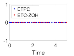
(a) Triggering instants

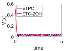
(b) Convergence of $V(x)$

Figure 2: Simulation results of Example 1.

Figure 2 presents the simulation results with $p=3$, $T=0.1$, $\delta=1$ and $x(0)=[0\quad 1\quad 0]^{T}$. Figure 2(a) presents the triggering time instants for the proposed ETPC method and zero-order-hold ETC (ETC-ZOH). We can see that the number of triggering instants is less for ETPC compared to ETC-ZOH. Figure 2(b) shows the evolution of $V(x)$ along the system trajectory for both the methods. Note that, $V(x)$ converges to the ultimate bound $\epsilon=0.05$ in both the cases.

Next, we analyze the effect of discount factor $\delta$ on the average inter-event time (AIET) and the minimum inter-event time (MIET). We calculate the AIET and the MIET over $1000$ events for different values of $\delta$ with $p=3$, $T=0.5$ and $x(0)=[0\quad 1\quad 0]^{T}$. Table I shows that the AIET and the MIET monotonically increase as the value of the discount factor decreases. Note that a smaller value of $\delta$ gives more priority to the short-term approximation error while solving the optimization problem (4). Thus, we observe an increase in the values of AIET and MIET as the value of $\delta$ decreases.

TABLE I: AIET and MIET, over $1000$ events, for different values of $\delta$ with $p=3$, $T=0.5$ and a given initial condition.

$\delta$	0.2	0.4	0.6	0.8
AIET	0.2216	0.2138	0.2092	0.2063
MIET	0.0057	0.0055	0.0054	0.0053

Next, we consider $100$ initial conditions uniformly sampled from the unit sphere and we calculate the AIET and the MIET over $100$ events for each initial condition with $T=0.3$, $p=3$, and $\delta=0.5$. The average of AIET over the set of initial conditions is observed as $0.0157$ and $0.3772$ for ETC-ZOH and ETPC, respectively. The minimum of MIET over the set of initial conditions is observed as $8.2744\times 10^{-4}$ and $0.0141$ for ETC-ZOH and ETPC, respectively. Note that the proposed control method provides a significant improvement in the values of AIET and MIET compared to the event-triggered zero-order-hold control method. We repeat the procedure for different values of $T$ and $p$, and the observations are tabulated in Table II. In Table II, we can see that there is a decreasing trend in the values of AIET and MIET as $T$ increases. Whereas, there is an increasing trend in AIET and MIET as $p$ increases.

TABLE II: Average of AIET and minimum of MIET, over a set of initial conditions, for different values of $T$ and $p$ with $\delta=0.5$.

	T
	0.4		0.6		0.8
p	AIET	MIET	AIET	MIET	AIET	MIET
3	0.2598	0.0074	0.1481	0.0037	0.0991	0.0025
4	0.3694	0.0220	0.2784	0.0071	0.1758	0.0044
5	0.3706	0.0242	0.3693	0.0181	0.3166	0.0075

Next, we also evaluate the performance of the proposed control method in the special case where the coefficients of the parameterized control input are determined by solving the finite horizon discrete time optimization problem given in Remark 6. Table III shows that there is a decreasing trend in AIET and MIET as the discrete time step size $T_{s}$ increases.

TABLE III: Average of AIET and minimum of MIET, over a set of initial conditions, for different values of $T_{s}$ with $T=NT_{s}=0.3$, $p=3$ and $\delta=0.5$.

$T_{s}$	0.01	0.02	0.03	0.05
AIET	0.3434	0.1752	0.1179	0.0889
MIET	0.0127	0.0005	0.0004	0.0003

V CONCLUSION

In this paper, we proposed the event-triggered parameterized control (ETPC) method for control of nonlinear systems with external disturbances. We designed a parameterized control law and an event-triggering rule that guarantee global uniform ultimate boundedness of the trajectories of the closed loop system and non-Zeno behavior of the generated inter-event times. Through numerical simulation, we compared the proposed control method with the existing event-triggered control based on zero-order-hold and showed a significant improvement in terms of the average inter-event time and the minimum inter-event time. Future work includes the generalization of this control method to distributed control setting, control under model uncertainty, quantization of the parameters, time delays, and a control Lyapunov function or MPC approach to ETPC.

References

- [1] D. Hercog, Communication protocols: principles, methods and specifications. Springer, 2020.
- [2] P. Tabuada, “Event-triggered real-time scheduling of stabilizing control tasks,” IEEE Transactions on Automatic Control, vol. 52, no. 9, pp. 1680–1685, 2007.
- [3] W. P. M. H. Heemels, K. H. Johansson, and P. Tabuada, “An introduction to event-triggered and self-triggered control,” in IEEE Conference on Decision and Control (CDC), 2012, pp. 3270–3285.
- [4] M. Lemmon, “Event-triggered feedback in control, estimation, and optimization,” in Networked control systems. Springer, 2010, pp. 293–358.
- [5] D. Tolić and S. Hirche, Networked control systems with intermittent feedback. CRC Press, 2017.
- [6] A. Anta and P. Tabuada, “To sample or not to sample: Self-triggered control for nonlinear systems,” IEEE Transactions on Automatic Control, vol. 55, no. 9, pp. 2030–2042, 2010.
- [7] W. P. M. H. Heemels, M. C. F. Donkers, and A. R. Teel, “Periodic event-triggered control for linear systems,” IEEE Transactions on Automatic Control, vol. 58, no. 4, pp. 847–861, 2013.
- [8] E. García and P. Antsaklis, “Model-based event-triggered control for systems with quantization and time-varying network delays,” IEEE Transactions on Automatic Control, vol. 58, pp. 422–434, 02 2013.
- [9] W. Heemels and M. Donkers, “Model-based periodic event-triggered control for linear systems,” Automatica, vol. 49, no. 3, pp. 698–711, 2013.
- [10] H. Zhang, D. Yue, X. Yin, and J. Chen, “Adaptive model-based event-triggered control of networked control system with external disturbance,” IET Control Theory & Applications, vol. 10, no. 15, pp. 1956–1962, 2016.
- [11] Z. Chen, B. Niu, X. Zhao, L. Zhang, and N. Xu, “Model-based adaptive event-triggered control of nonlinear continuous-time systems,” Applied Mathematics and Computation, vol. 408, p. 126330, 2021.
- [12] L. Zhang, J. Sun, and Q. Yang, “Distributed model-based event-triggered leader–follower consensus control for linear continuous-time multiagent systems,” IEEE Transactions on Systems, Man, and Cybernetics: Systems, vol. 51, no. 10, pp. 6457–6465, 2021.
- [13] H. Li and Y. Shi, “Event-triggered robust model predictive control of continuous-time nonlinear systems,” Automatica, vol. 50, no. 5, pp. 1507–1513, 2014.
- [14] F. D. Brunner, W. Heemels, and F. Allgower, “Robust event-triggered MPC with guaranteed asymptotic bound and average sampling rate,” IEEE Transactions on Automatic Control, vol. 62, no. 11, p. 5694 – 5709, 2017.
- [15] H. Li, W. Yan, and Y. Shi, “Triggering and control codesign in self-triggered model predictive control of constrained systems: With guaranteed performance,” IEEE Transactions on Automatic Control, vol. 63, no. 11, pp. 4008–4015, 2018.
- [16] A. Li and J. Sun, “Resource limited event-triggered model predictive control for continuous-time nonlinear systems based on first-order hold,” Nonlinear Analysis: Hybrid Systems, vol. 47, p. 101273, 2023.
- [17] K. Hashimoto, S. Adachi, and D. V. Dimarogonas, “Self-triggered model predictive control for nonlinear input-affine dynamical systems via adaptive control samples selection,” IEEE Transactions on Automatic Control, vol. 62, no. 1, pp. 177–189, 2017.
- [18] B. Demirel, V. Gupta, D. E. Quevedo, and M. Johansson, “On the trade-off between communication and control cost in event-triggered dead-beat control,” IEEE Transactions on Automatic Control, vol. 62, no. 6, pp. 2973–2980, 2017.
- [19] C. Nowzari and J. Cortés, “Team-triggered coordination for real-time control of networked cyber-physical systems,” IEEE Transactions on Automatic Control, vol. 61, no. 1, pp. 34–47, 2016.
- [20] J. Liu, Y. Yu, H. He, and C. Sun, “Team-triggered practical fixed-time consensus of double-integrator agents with uncertain disturbance,” IEEE Transactions on Cybernetics, vol. 51, no. 6, pp. 3263–3272, 2021.
- [21] A. B. Chammas and C. T. Leondes, “On the design of linear time invariant systems by periodic output feedback part i. discrete-time pole assignment,” International Journal of Control, vol. 27, no. 6, pp. 885–894, 1978.
- [22] P. Kabamba, “Control of linear systems using generalized sampled-data hold functions,” IEEE Transactions on Automatic Control, vol. 32, no. 9, pp. 772–783, 1987.
- [23] J. Lavaei, S. Sojoudi, and A. G. Aghdam, “Pole assignment with improved control performance by means of periodic feedback,” IEEE Transactions on Automatic Control, vol. 55, no. 1, pp. 248–252, 2010.
- [24] A. Rajan and P. Tallapragada, “Event-triggered parameterized control for stabilization of linear systems,” Accepted at 62nd IEEE Conference on Decision and Control (CDC), 2023.
- [25] A. Rajan, V. Harini, B. Amrutur, and P. Tallapragada, “Event-triggered polynomial control for trajectory tracking of unicycle robots,” arXiv preprint arXiv:2308.15834, 2023. [Online]. Available: http://arxiv.org/abs/2308.15834