Red Asymmetry of H_α Line Profiles during the flares on the active RS CVn-type star II Pegasi

Abstract

Stellar coronal mass ejections (CMEs) have recently attracted much attention for their impacts on stellar evolution and surrounding exoplanets. RS CVn-type stars could produce large flares, and therefore may have frequent CMEs. Here we report the capture of a possible CME or chromospheric condensation on the RS CVn-type star II Pegasi (II Peg) using high-resolution spectroscopic observation. Two flares were detected during the observation, and the low limits of the flare energies are of the order of $10^{33}$ erg and $10^{34}$ erg, respectively. Using mean spectrum subtraction, the H_α residual shows red asymmetry during the flares, and the redshifted broad emission components are probably caused by chromospheric condensation or coronal rain. Moreover, a far redshifted extra emission component with a high bulk velocity of 429 km s^-1 was observed during the second flare and is probably due to a prominence eruption. The velocity greatly exceeds the star’s escape velocity, which means that this eruption can develop into a CME. The CME mass is estimated to be 0.83–1.48 $\times~{}10^{20}$ g, which is slightly larger than the value expected from solar flare-CME extrapolation. The kinetic energy of CME, derived to be 0.76–1.15 $\times~{}10^{35}$ erg, is less than the kinetic energy extrapolated from solar events. Additionally, we could not completely rule out the possibility of chromospheric condensation resulting in the far redshifted extra emission. Finally, there is a blueshifted broad component in the subtracted H_α profile derived using synthesized spectral subtraction when no flare happened, and its behavior is associated with the H_α activity features.

1 Introduction

Starspots, plages, flares, and prominences have been widely observed in cool stars (Schrijver & Zwaan, 2000). It is commonly accepted that all of these active phenomena arise from a powerful magnetic dynamo generated by the interplay between the turbulent motion in the convection zone and the stellar differential rotation, in a manner similar to the solar case. In recent years, stellar coronal mass ejections (CMEs) have attracted much attention, though they are more difficult to observe with current instrumentation because of having no spatial resolution. Based on some indirect evidences, such as Doppler-shifted emission or absorption signature in the optical, UV and X-ray spectral lines (e.g., Houdebine et al., 1990; Leitzinger et al., 2011; Argiroffi et al., 2019; Namekata et al., 2021; Inoue et al., 2023), X-ray, extreme-UV (EUV), and far-UV (FUV) dimming (e.g., Veronig et al., 2021; Namekata et al., 2023), and X-ray continuous absorption (e.g., Favata & Schmitt, 1999; Moschou et al., 2017), researchers have made a lot of attempts to detect stellar CME events. Frequently occurred CMEs may be an important contribution to mass and angular momentum loss in the course of stellar evolution (e.g., Aarnio et al., 2012; Osten & Wolk, 2015), and have severe impacts on the atmospheres of surrounding exoplanets (e.g., Airapetian et al., 2016; Cherenkov et al., 2017; Hazra et al., 2022).

RS CVn-type binary system includes at least one cool component showing particularly intense magnetic activity in several forms (Hall, 1976; Fekel et al., 1986). For example, prominence-like features have been detected in several RS CVn-type stars (e.g., Hall et al., 1990; Hall & Ramsey, 1992; Cao et al., 2019, 2020). Therefore, prominences may be common phenomena in this type stars. Moreover, RS CVn-type star has been frequently observed to produce strong flares and even superflares ($\gtrsim~{}10^{33}$ erg) (e.g., Tsuboi et al., 2016; Inoue et al., 2023). We detected a series of possibly associated magnetic activity phenomena in a short time, including flare-related prominence activation, a strong optical flare, and post-flare loops, on RS CVn-type star SZ Psc (Cao et al., 2019). Based on the well-defined connection between highly energetic flares and CMEs on the Sun and the close relation between CMEs and eruptive prominences, it can be hypothesized that RS CVn-type stars may have frequent CME occurrences. Here we focus on one of the most active and extensively studied single-lined RS CVn-type binary stars, II Peg.

The system II Peg (= HD 224085) consists of a K2 IV primary star and an unseen companion in an almost circular orbit with a period of about 6.7 days. The basic physical parameters of the K2 IV primary star are summarized in Table 1. The K2 IV star shows remarkable photometric variability caused by large starspots (e.g., Vogt, 1981; Lindborg et al., 2013), Ca ii H&K and H_α line emission (e.g., Vogt, 1981; Huenemoerder & Ramsey, 1987; Montes et al., 1997; Berdyugina et al., 1999; Frasca et al., 2008), and UV and X-ray radiation (e.g., Byrne et al., 1989; Ercolano et al., 2008). Moreover, II Peg belongs to stars to which Doppler imaging (DI) and Zeeman-Doppler imaging (ZDI) techniques were widely applied (e.g., Gu et al., 2003; Lindborg et al., 2011; Hackman et al., 2012; Kochukhov et al., 2013; Xiang et al., 2014; Rosén et al., 2015; Strassmeier et al., 2019).

Table 1: Basic Parameters of the K2 IV Primary Star of II Peg

Parameter	Value	Reference
Spectral Type	K2 IV	Strassmeier et al. (1993)
$V_{max}$ (mag)	7.2	Strassmeier et al. (1993)
$d$ (pc)	39.12 $\pm$0.08	Gaia Collaboration (2020)
$P_{orb}$ (days)	6.7242078	Rosén et al. (2015)
$P_{rot}$ (days)	6.7242078	Rosén et al. (2015)
$T_{eff}$ (K)	4750 K	Rosén et al. (2015)
$log~{}g$ (cgs)	3.5	Rosén et al. (2015)
$vsini$ (km s-1)	21.6	This work
$M$ (M☉)	0.8	Berdyugina et al. (1998)
$R$ (R☉)	3.4	Berdyugina et al. (1998)

Note. — $V_{max}$ is maximum brightness in V-band, $d$ is stellar distance, $P_{orb}$ is orbital period, $P_{rot}$ is rotation period, $T_{eff}$ is effective temperature, $log~{}g$ is Log gravity, $vsini$ is projected rotational velocity, $M$ is mass, and $R$ is radius.

II Peg is a high-rate flaring star. Flares have been reported several times over a wide range of wavelength regions, such as optical, UV, and X-ray bands (e.g., Rodono et al., 1987; Doyle et al., 1991; Berdyugina et al., 1999; Frasca et al., 2008; Ercolano et al., 2008; Siwak et al., 2010; Tsuboi et al., 2016). In the optical spectral lines, sudden enhancements of the H_α and Ca ii lines, as well as the emission feature in the He i D₃ line, were usually attributed to flare events. For example, Berdyugina et al. (1999) detected two strong optical flares using the He i D₃, Ca ii K, and Ca ii $\lambda$8498 lines. Broad blueshifted emissions could be found in the He i D₃ and Ca ii K line profiles at the flare maximum, which were attributed to the process of the explosive evaporation from the low chromosphere.

In this paper, we present the results about strong optical flares and flare-associated activity phenomena on II Peg. In Section 2, we provide details of our high-resolution spectroscopic observation and data reduction. The analysis of chromospheric activity indicators covered in observed spectra is described in Section 3. In Section 4, the behavior of chromospheric activity indicators and the associated magnetic activity phenomena of II Peg during our observation are discussed in more detail. Finally, we give a summary and conclusions in Section 5.

2 Spectroscopic observation and data reduction

Spectroscopic data of II Peg were obtained over nine nights from 2016 January 22 to 31. The observation was carried out with the fiber-fed high-resolution spectrograph (HRS), installed on the 2.16 m telescope at the Xinglong station of the National Astronomical Observatories, Chinese Academy of Sciences, China (Fan et al., 2016). HRS produces spectra with a resolving power R = $\lambda$/$\Delta\lambda$ $\simeq$ 48000 in a wavelength range of 3900–10000 Å, using a $4096\times 4096$ pixel CCD detector.

Table 2 lists the information of our observation, which includes the observing date, exposure time, heliocentric Julian date (HJD), and orbital phase calculated with the ephemeris:

$$HJD=2,448,942.428+6^{d}.7242078\times E$$ (1)

from Rosén et al. (2015), where the zero-point is a time of the K2 IV primary star of II Peg having maximum positive radial velocity. In addition, we observed some slowly rotating, inactive stars with the same spectral type and luminosity class as II Peg. They are required for the spectral subtraction technique described in Section 3.1.

Data reduction was performed with the IRAF package, following the standard procedures (image trimming, bias correction, flat-field division, scattered light subtraction, one-dimensional spectrum extraction, and wavelength calibration). The wavelength calibration was obtained by using emission lines of Th-Ar spectra of the corresponding nights. Finally, all spectra were normalized by using low-order polynomial fits to the observed continuums with the CONTINUUM task in the IRAF package.

Examples of the normalized Ca ii IRT ($\lambda$8662, $\lambda$8542, and $\lambda$8498), He i $\lambda$6678, H_α, Na i D₁, D₂ doublet, He i D₃, and H_β line profiles of II Peg are displayed in Figure 1.

Table 2: II Peg Observing Log

Date	Exp.time	HJD	Phase
	(s)	(2,450,000+)
2016 Jan 22	1800	7409.944	0.259
2016 Jan 22	1800	7409.968	0.262
2016 Jan 23	1800	7410.943	0.407
2016 Jan 23	1800	7410.966	0.410
2016 Jan 24	1800	7411.949	0.557
2016 Jan 24	1800	7411.972	0.560
2016 Jan 25	1800	7412.935	0.703
2016 Jan 25	1200	7412.992	0.712
2016 Jan 27	1200	7414.931	0.000
2016 Jan 27	1200	7415.016	0.013
2016 Jan 28	1800	7415.937	0.150
2016 Jan 28	1800	7416.012	0.161
2016 Jan 29	1800	7416.939	0.299
2016 Jan 29	1800	7416.962	0.302
2016 Jan 30	1800	7417.971	0.452
2016 Jan 30	1800	7417.995	0.456
2016 Jan 31	1800	7418.941	0.597
2016 Jan 31	1200	7418.985	0.603
2016 Jan 31	1800	7419.012	0.607

Note. — HJD and phase are calculated for mid-exposure of each observation.

3 Spectral analysis

Several chromospheric activity indicators, namely Ca ii IRT, He i $\lambda$6678, H_α, Na i D₁, D₂ doublet, He i D₃, and H_β lines, formed in a wide range of atmospheric heights from the region of temperature minimum to the upper chromosphere, are covered in our echelle spectra and therefore analyzed, especially the H_α line.

As shown in Figure 1, clear central emission features appear in the cores of the Ca II IRT absorption line profiles. Moreover, the H_α line is always in emission above the continuum and has a significant variable profile during our observation. The Na i D₁, D₂ doublet lines are characterized by deep absorption features. The H_β line often shows strong filled-in features and exhibits emission above the continuum for some of our spectra when the He i D₃ line shows strong emission.

3.1 Synthesized spectral subtraction

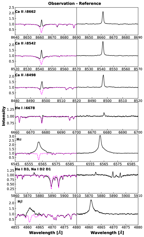
Figure 1: Examples of the observed, synthesized, and subtracted spectra for the Ca ii $\lambda$8662, Ca ii $\lambda$8542, and Ca ii $\lambda$8498, He i $\lambda$6678, H_α, Na i D₁, D₂ doublet, He i D₃, and H_β line spectral regions, shown for one spectrum obtained at phase 0.597 on 2016 January 31. For the left part of each panel, the black solid line is the observed spectrum, and the magenta dashed line represents the synthesized spectrum constructed from spectrum of a reference star. The resulting subtraction spectrum is displayed in the right part of each panel. The label identifying each chromospheric activity indicator is marked in the corresponding panel.

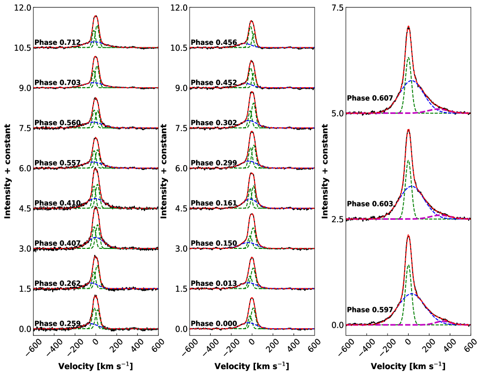
Figure 2: Gaussian fitting (dashed lines) for the subtracted H_α line profiles (black solid lines). The corresponding phases are marked, and all the spectra are corrected to the rest velocity frame of the K2 IV primary component of II Peg.

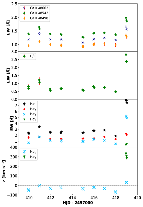
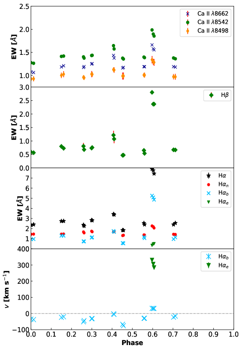
Figure 3: Measurements of the subtracted Ca ii IRT, H_α, and H_β line profiles vs. HJD (left panel) and orbital phase (right panel). For each panel, from top to bottom: the EWs of the subtracted Ca ii IRT line profiles, the EWs of the subtracted H_β line profiles, the EWs of the subtracted total H_α line profiles and the fitted narrow, broad, and extra emission components, and the velocities of the broad and extra emission components in the subtracted H_α line profiles. H_αe represents the extra emission component in the subtracted H_α line profile. The gray dashed-dotted line indicates the zero-point of velocity.

To determine the pure activity contribution in these chromospheric sensitivity lines, we apply a spectral subtraction technique to remove the underlying photospheric contribution by making use of the STARMOD program (Barden, 1985; Montes et al., 1997, 2000). We have widely used this technique for chromospheric activity studies and the detection of prominence-like events in active binary systems (e.g., Gu et al., 2002; Cao & Gu, 2015; Cao et al., 2019, 2022).

Since II Peg is a single-lined binary star, we use only one reference star spectrum to reproduce the synthesized spectrum. By comparison, the spectrum of the inactive star HR 3351 (K0 IV) is used as reference in the synthesized spectrum construction. The rotational velocity ($vsini$) value is determined by using the reference spectrum based on the method described in detail by Barden (1985). The value of 21.6 km s^-1 is obtained from high signal to noise ratio (S/N) spectra, spanning the wavelength regions 6330–6500 Å with many photospheric absorption lines, which is in good agreement with the results estimated by several authors (e.g., Berdyugina et al., 1998; Rosén et al., 2015; Strassmeier et al., 2019). Consequently, the synthesized spectra are constructed by rotationally broadening the reference spectrum to the $vsini$ value derived above and shifting along the radial-velocity axis, to get best fits. Then, the subtracted spectra between the observed and synthesized ones are calculated, which represent the pure activity contribution of II Peg. Here, we can also obtain the radial velocities of the K2 IV primary star relative to the reference star at each observation phase, and these values are then used to calibrate the radial velocity variations due to orbital motion in the following analysis.

As a typical example, we illustrate the above-described processing in Fig. 1, too. The synthesized spectra match the observational spectra quite well except the Na i D₁, D₂ doublet lines. Because they are sensitive to the effective temperature, a slight temperature difference between HR 3351 and II Peg would produce larger changes in the wings of the Na i D₁, D₂ doublet line profiles.

The equivalent widths (EWs) of the subtracted Ca ii IRT, H_α, and H_β line profiles are measured, as described in our previous papers (Cao & Gu, 2015, 2017; Cao et al., 2019), and summarized in Table A1 together with their uncertainties. The ratios of the EW($\lambda$8542)/EW($\lambda$8498) and the E_Hα/E_Hβ are also provided in Table A1. The E_Hα/E_Hβ ratios are calculated from the EW(H_α)/EW(H_β) values with the correction (see Hall & Ramsey, 1992), which takes into account the absolute flux density in H_α and H_β lines, and the color index.

During our observation of II Peg, the EW₈₅₄₂/EW₈₄₉₈ ratios are in the range of 1–2, which suggests that the Ca ii IRT line emission arises predominantly from plage-like regions (e.g., Montes et al., 2000; Gu et al., 2002; Cao & Gu, 2015; Cao et al., 2023). The E_Hα/E_Hβ ratios are usually used as diagnostic for discriminating between prominences and plages on the stellar surface. According to the results of Hall & Ramsey (1992), the low ratios ($\sim$ 1–2) could be achieved both in plages and prominences viewed against the stellar disk, but high values ($\sim$ 3–15) could only be achieved in prominence-like structures viewed off the stellar limb. Therefore, the high ratio ($\gtrsim$ 3) that we found in II Peg suggests that the emission probably arose from extended prominence-like regions.

With the H_α subtraction, showing in Fig. 2, we model the line profile by Gaussian fitting. In general, the flaring H_α spectra could not simply be fitted by Gaussian profile, as their wing can be well fitted with Lorenzian-like profile due to the strong Stark broadening (Kowalski et al., 2017; Namekata et al., 2020). For our situation, it can be seen that the profile may be well fitted by using several Gaussian profile components. In addition to the narrow components, there is a blue- or redshifted broad component having a full width at half maximum (FWHM) of 150–307 km s^-1. For most of the subtracted spectra, two narrow components are needed in fitting. This is reasonable, because the distribution of chromospheric activity regions is not uniformly expressed on the stellar surface. Moreover, for spectra taken at phases 0.597, 0.603, and 0.607 on 2016 January 31 (see the rightmost panel of Fig. 2), it is noteworthy that there is a far-redshifted extra emission component (shown by the magenta dashed-dotted line) in the subtraction, except a narrow and a strong redshifted broad components. Here, just one narrow component is used in fitting, probably because a large flare region dominates the activity of II Peg at these observing phases. In Table A1, we also list the EWs of the broad and narrow components, and the velocities of the broad component.

Finally, we plot the measurements listed in Table A1 as functions of HJD and orbital phase in Fig. 3, respectively, together with the EWs, and velocities of the far-redshifted extra emission component in the subtracted H_α line. It can be seen that the EW variations of the different chromospheric activity indicators are closely correlated, similar to the behavior of many chromospherically active stars.

3.2 Mean spectrum subtraction

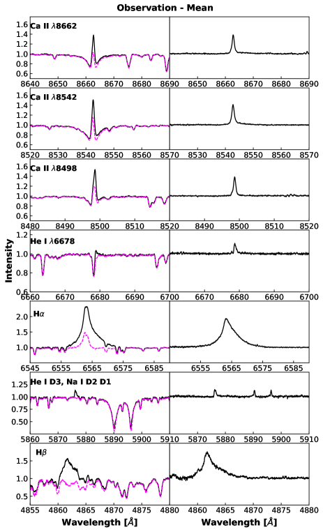
Figure 4: Same as Fig. 1, but for subtracting a mean spectrum (magenta dashed line) from the observed spectrum for each chromospheric activity indicator.

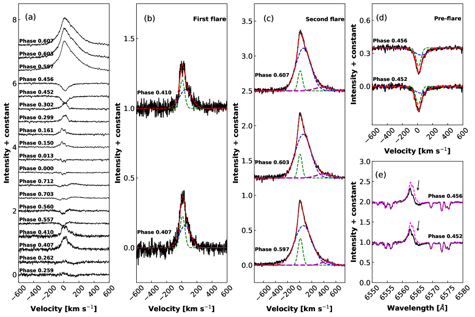
Figure 5: The H_α residuals between the observed and mean spectra. (a) All residuals at different phases during our observation, (b) and (c) Gaussian fitting (dashed lines) for the residuals during two flares (solid lines), (d) Gaussian fitting (dashed lines) for the residuals during pre-flare, (e) the observed pre-flare spectra (solid lines) compared with the mean spectrum (magenta dashed lines). The corresponding phases are marked in each panel, and arrows indicate extra absorption features in the red wings of the observed H_α line profiles. The residual spectra are corrected to the rest velocity frame of the K2 IV primary component of II Peg.

There are two strong optical flare events detected during our observation, which are discussed in Sec. 4.1 in more detail. Typically, a pre-flare spectrum subtraction is performed to analyze the flaring spectra (e.g., Namekata et al., 2021; Inoue et al., 2023). In our situation, however, because the closest pre-flaring spectra were taken the night before, and because the chromospheric line profile of II Peg would change significantly between different nights, we subtract a mean spectrum from the observed spectra to analyze the behavior of the chromospheric lines during the flares and to identify whether the H_α asymmetry is associated with the flares. We first correct all the spectra so that they are aligned, and then the mean spectrum is obtained from spectra except ones taken during the two flares. Therefore, the mean spectrum could represent the mean activity state of II Peg when no flare happens. To a certain extent, the residuals of the two flares can reflect the flare behavior also the flare-related activity phenomena. An example for illustrating this process is displayed in Fig. 4.

Fig. 5(a) exhibits all the H_α residuals between the observed and mean spectra, and as shown in Fig. 5(b)–(d), we model the residual profiles obtained during two flares (observed on 2016 January 23 and 31, respectively) and the pre-flare of the second flare (observed on 2016 January 30) by using Gaussian fitting. For the first flare, the residual spectra are modeled by a narrow Gaussian profile component and a redshifted broad component with a bulk velocity of about 40–50 km s^-1. The pre-flare residuals of the second flare show absorption features and red asymmetry, which could be modeled by a narrow Gaussian absorption component and a slightly redshifted broad absorption component. The absorption feature is not just because II Peg has a lower chromospheric activity at these observing phases when comparing with the mean activity state. A probable reason is that there is an extra absorption in the red wing of the H_α line profile, as indicated through comparing the observed and mean spectra in Fig. 5(e). For the second flare, the residual spectra are similar with the STARMOD subtraction, which still can be modeled by using a weak narrow, a redshifted strong broad, and a far-redshifted extra emission components. The bulk velocity of the redshifted broad emission component is around of 60 km s^-1, while the far-redshifted extra emission component has a bulk velocity decreased from 429 km s^-1 to 376 km s^-1, and could extends its velocity up to 600–650 km s^-1 during our observations. Moreover, the extra emission becomes more and more prominent, with the FWHM increased from 206 km s^-1 to 307 km s^-1.

On the whole, during the two flares, our analytical method demonstrates that the H_α red asymmetry is closely related to flaring activity. Hereafter, all investigations and calculations for the flare and flare-associated (especially the possible CME event discussed in Section. 4.2) events are based on the results of mean spectrum subtraction.

4 Results and discussion

4.1 Flares and flare energies

Table 3: EWs, Surface Fluxes, and Flare Luminosities of the Residuals of Chromospheric Activity Lines at Flare Maximums

Line	EW	Fs ($\times~{}10^{7}$)	L ($\times~{}10^{30}$)
	(Å)	(erg cm-2 s-1)	(erg s-1)
Flare on 2016 Jan 23
$\mbox{Ca~{}{\sc ii}}~{}\lambda 8662$	0.208$\pm$0.015	0.04	0.30
$\mbox{Ca~{}{\sc ii}}~{}\lambda 8542$	0.215$\pm$0.014	0.05	0.32
$\mbox{Ca~{}{\sc ii}}~{}\lambda 8498$	0.114$\pm$0.033	0.02	0.17
$\mbox{He~{}{\sc i}}~{}\lambda 6678$	0.047$\pm$0.012	0.01	0.09
Hα	0.887$\pm$0.097	0.23	1.65
Hβ	0.705$\pm$0.082	0.17	1.16
Total lines			3.69
Flare on 2016 Jan 31
$\mbox{Ca~{}{\sc ii}}~{}\lambda 8662$	0.513$\pm$0.002	0.11	0.74
$\mbox{Ca~{}{\sc ii}}~{}\lambda 8542$	0.622$\pm$0.002	0.13	0.92
$\mbox{Ca~{}{\sc ii}}~{}\lambda 8498$	0.394$\pm$0.004	0.08	0.59
$\mbox{He~{}{\sc i}}~{}\lambda 6678$	0.093$\pm$0.014	0.02	0.17
Hα	5.714$\pm$0.145	1.51	10.63
Na i D1	0.075$\pm$0.019	0.02	0.14
Na i D2	0.086$\pm$0.023	0.02	0.16
He i D3	0.155$\pm$0.015	0.04	0.29
Hβ	2.467$\pm$0.033	0.58	4.06
Total lines			17.11

Stellar flares are dramatic explosive phenomena in the outer atmosphere of active stars, commonly believed to be caused by the energy released in magnetic reconnection. Flares can be observed across the entire electromagnetic spectrum from shorter X-ray to longer radio wavelengths. In the optical spectral region, the He i D₃ line is an important and commonly used indicator to trace flare activity in solar and stellar chromospheres because of its very high excitation potential. When flares happen, the He i D₃ line shows an obvious emission feature above the continuum level, as widely observed during flares on the Sun (Zirin, 1988) and several RS CVn-type stars (e.g., Gu et al., 2002; García-Alvarez et al., 2003; Cao et al., 2019).

Two optical flare events were detected during our observations. The first flare was observed at phases 0.407 and 0.410 on 2016 January 23, while the second one occurred at phases 0.597, 0.603, and 0.607 on 2016 January 31. The second flare is much stronger than the first one (see Table 3 and Figure 3). During two optical flares, the He i D₃ line shows an obvious emission feature and the H_α line and other activity lines display stronger emission. Moreover, another He i line, $\lambda$6678, also shows a distinct emission feature, especially after subtracting the synthesized spectrum or the mean spectrum. A typical example of flaring spectrum could be found in Figure 1 or Figure 4.

We did not capture the whole life cycle of the two flares of II Peg due to limited observations. Since the flare intensity shows a decreasing trend, our observations were part of the gradual decay phases of flares and the observations at phases 0.407 and 0.597 could be considered as the emission maxima of two flares. We compute the stellar continuum flux $F_{H{\alpha}}$ (in erg cm^-2 s^-1 Å^-1) near the H_α line as a function of the color index $B-V$ ($\sim$ 1.031 for II Peg; Messina 2008) based on the empirical relationship:

$$\log{F_{H{\alpha}}}=[7.538-1.081(B-V)]\pm{0.33}$$

$$0.0~{}\leq~{}B-V~{}\leq~{}1.4$$ (2)

of Hall (1996), and then convert the EW into an absolute surface flux $F_{S}$ (in erg cm^-2 s^-1). Following the method adopted by Montes et al. (1999), García-Alvarez et al. (2003), and Cao et al. (2019), we obtain the stellar continuum fluxes $F_{\lambda}$ for the other chromospheric activity lines by using the flux ratios:

$$\frac{F_{6563}}{F_{\lambda}}~{}=~{}\frac{B_{6563}(T)}{B_{\lambda}(T)}$$ (3)

where B($\lambda$, T) is the Plank function. The flux ratios are given by assuming a blackbody with contribution of the K2 IV primary of II Peg at the effective temperature $T_{eff}$ = 4750 K. Then, we convert these fluxes into luminosities using the stellar radius $R_{\star}$ = 3.4$R_{\sun}$. The corresponding EWs, surface fluxes, and luminosities at flare maxima in the residuals of each chromospheric activity line are listed in Table 3. For the first flare, because the flare emission in the Na i D₁, D₂ doublet and He i D₃ lines is very weak and the spectrum has low S/N, we do not measure them. The H_α luminosities of two flares are of similar order of magnitude as strong flares on other highly active RS CVn-type stars, such as V711 Tau (Cao & Gu, 2015), UX Ari (Montes et al., 1996; Gu et al., 2002; Cao & Gu, 2017), HK Lac (Catalano & Frasca, 1994), SZ Psc (Cao et al., 2019, 2020), and RS CVn (Cao et al., 2023), especially for the second flare.

Moreover, in Table 3, we also provide the total luminosities summed from observed chromospheric activity lines. For our observation, it is impossible to estimate the flare duration from the initial outburst to the end, but we can give a timescale of 1800 seconds for two optical flares, respectively. The duration times of two flares are just the exposure times of our observations, which means they are underestimated. Thus, the estimated total energies released in optical chromospheric lines are $6.6~{}\times~{}10^{33}$ erg for the first flare and $3.1~{}\times~{}10^{34}$ erg for the second one. These values represent the low limits of the flare energies and are comparable to those of stellar superflares, particularly the second flare.

4.2 H_α profile asymmetry during the flares

4.2.1 Interpretation of H_α profile asymmetry

In the case of solar flares, as discussed by Moschou et al. (2019), Koller et al. (2021), and Wu et al. (2022), the redshifted H_α emission may arise from coronal rain, or from chromospheric condensation, or from prominence/filament eruption with a backward direction. The red asymmetry of H_α profile may be caused by one of these three possible scenarios or their combinations. It is difficult to distinguish them because the events are not spatially resolved. One possible way to identify them is based on the Doppler shifts. Firstly, coronal rain is dense and cool plasma condensation formed in the hot corona, and then falls down along post-flare loops to the solar surface with average velocity of about 60–70 km s^-1 (Antolin et al., 2012; Lacatus et al., 2017). A flare-driven coronal rain was reported with a velocity up to 134 km s^-1 by Martínez Oliveros et al. (2014) and the downward acceleration is generally not more than 80 m s^-2. Secondly, chromospheric condensation is usually observed with a typical downflow velocity of tens of kilometers per second (Ichimoto & Kurokawa, 1984). And such condensation usually occurs during the impulsive phase of solar flare and is caused by nonthermal heating processes in flares. Finally, the typical velocity of solar prominence/filament eruption is in the range of 10–500 km s^-1. And as discussed by Wu et al. (2022), a detectable backward prominence/filament eruption requires specially spatial location, which implies that its occurrence is very rare.

During our two flares, there are the redshifted broad emission components with a bulk velocity of about 40–50 km s^-1 for the first flare and about 60 km s^-1 for the second one. The velocities of the redshifted broad components correspond well to the velocity of chromospheric condensation and coronal rain in the solar case. This suggests that chromospheric condensation or coronal rain is responsible for their occurrence.

During the second flare, the far-redshifted extra emission component has a large velocity decreased from 429 km s^-1 to 376 km s^-1 and could extends its velocity up to 600–650 km s^-1, which is significant larger than the typical velocities of coronal rain and chromospheric condensation in solar case. And, the velocity approaches the larger value of solar prominence/filament eruption. Thus, stellar prominence eruption might be a good explanation for its origination based on what is known about the Sun. Moreover, there is a scenario for supporting its occurrence. As analyzed in Section 3.2, for the pre-flare spectra, absorption features appear in the residuals. Part of the absorption, especially the extra absorption in the red wing of the H_α line, could be caused by a stellar prominence projected on the right hemisphere of the star, and therefore scattered the underlying chromospheric activity emission out of the line of sight (Collier Cameron & Robinson, 1989). On the next observing night, after the K2 IV primary star rotated about 50^∘ from phase 0.456 to phase 0.597, it is possible that the corotated prominence moved close to the limb of the stellar disk and then occurred a backward eruption due to a superflare. An alternate scenario can be that the prominence just moved to the opposite hemisphere, and then a forward eruption occurred. When the eruption began to extend outward, we just observed them. In both cases, the flare must happened around the limb of the stellar disk, where at least one of its footpoints which produced H_α emission can be seen by us. Just at these specially spatial locations, stellar prominence eruption could result in a redshifted emission feature, which is consistent with the situation discussed by Wu et al. (2022) and the scenario depicted in the second panel of Figure 4 of Moschou et al. (2019), respectively.

Prominence/filament eruption can lead to CME, especially when the eruption velocity is sufficiently large. In a superflare, for example, Inoue et al. (2023) detected a blueshifted excess emission component of the H_α line on RS CVn-type star V1355 Orionis. Because the velocity greatly exceeds the star’s escape velocity, it could be thought to originate from prominence eruption and could develop into a CME. Due to projection effects, however, our measured velocity only is the lower limit of the true velocity of eruption. For the eruption scenarios discussed above, there may be a larger angle between the eruption direction and the line of sight, and therefore the prominence eruption has a small velocity component along the line of sight. For the K2 IV primary star of II Peg, the escape velocity $v_{esp}~{}=~{}630(\frac{M_{\star}}{M_{\sun}})^{1/2}(\frac{R_{\star}}{R_{\sun}})^{-1/2}$ km s^-1 can be determined to be about 306 km s^-1 at the surface of the star. Therefore, for our situation, the underestimated velocity is still much larger than the star’s escape velocity, which provides a very important evidence that this stellar prominence eruption can develop into a successful CME event.

The energy scale of the flares on II Peg vastly exceeds that of typical solar flares. This suggests that, while similar mechanisms may operate during the flares, the magnitude of redshift phenomena could differ greatly between solar flares and flares on stars. Namizaki et al. (2023) observed the H_α red asymmetry during a superflare on an active M dwarf, YZ Canis Minoris. The velocity of the red asymmetry is much fast ranging from 200–500 km s^-1, which could be interpreted as chromospheric condensation heated by nonthermal electrons. Through the numerical simulations, moreover, Longcope (2014) suggested that strong heating fluxes during large superflares could produce fast chromospheric condensation. For our situation, the far-redshifted extra emission is accompanied by the prominent line broadening (see Section 3.2), which probably suggests the appearance of chromospheric condensation due to nonthermal heating during the flare decay. Although the velocity of the far-redshifted extra emission is much high, therefore, we can not entirely rule out the possibility of chromospheric condensation.

In addition, it is estimated that the flare loop size is considerably larger in the case of superflares on RS CVn-type stars (e.g, Tsuboi et al., 2016). Consequently, the velocity of falling plasma along loops during coronal rain for RS CVn-type stars could be much higher than those in solar flares. In the solar case, the falling materials move downward along loops with an acceleration of about $g_{eff}$/3 and its maximum velocity is about 100 km s^-1 (Antolin, 2020). According to the method of Wu et al. (2022), the maximum velocity of the falling plasma on II Peg is estimated to be about 63 km s^-1 on the assumption that the propagation distance scales with the radius of the star. Tsuboi et al. (2016) proposed that the largest loop size from II Peg are much larger than the binary separation. If we assume that the propagation distance of coronal rain is the binary separation of II Peg ($\sim$15.6 R_☉), the maximum velocity is about 134 km s^-1. The velocity of falling plasma is much smaller than the velocity of the far-redshifted emission during the flare of II Peg, and therefore we could eliminate the possibility of coronal rain.

4.2.2 Mass of the possible CME

By following Houdebine et al. (1990) and Koller et al. (2021), mass of the CME can be estimated as:

$$M_{CME}~{}\geqslant~{}\frac{4{\pi}d^{2}f_{line}m_{H}}{A_{ji}h\nu_{ji}P_{esc}}\frac{N_{tot}}{N_{j}}$$ (4)

in which $d$ is the distance from the star, $f_{line}$ is the corresponding line flux from the CME emission feature, $m_{H}$ is the mass of a hydrogen atom, $N_{tot}/N_{j}$ is the ratio between the number density of hydrogen atoms and the number density of hydrogen atoms at excited level $j$, $h$ is the Planck constant, $\nu_{ji}$ and $A_{ji}$ are the frequency and Einstein coefficient for a spontaneous decay from level $j$ to $i$, and $P_{esc}$ is the escape probability.

In the calculation, we use the same parameter settings and same strategy as Koller et al. (2021). Due to a lack of $N_{tot}/N_{j}$ value for the H_α line ($j$ = 3, $i$ = 2) in the literature, they estimated $M_{CME}$ from the H_γ line ($j$ = 5, $i$ = 2) flux and then transformed to the H_α line by adopting a Balmer decrement of three (Butler et al., 1988). Houdebine et al. (1990) performed non-LTE modeling for a well-known flaring dMe star AD Leo and estimated $N_{tot}/N_{5}$ = $2~{}\times~{}10^{9}$. A typical value of 0.5 is used for $P_{esc}$, which indicates that half of the radiation escapes from the moving feature (Leitzinger et al., 2014). $A_{ji}$ is $2.53~{}\times~{}10^{6}$ for the H_γ line (Wiese & Fuhr, 2009).

Adopting the same strategy as Wu et al. (2022), we use the luminosity $L_{line}$ to instead of $4{\pi}d^{2}f_{line}$, because we also do not have absolute flux calibration. We have obtained the EW and luminosity of H_α at flare maximum (see Table 3), and then derived the $L_{line}$ according to the EW of the far red-shifted extra emission component. Finally, we calculate the mass of CME, which is in the range of 0.83–1.48 $\times~{}10^{20}$ g from our three exposures.

4.2.3 Comparison with other events

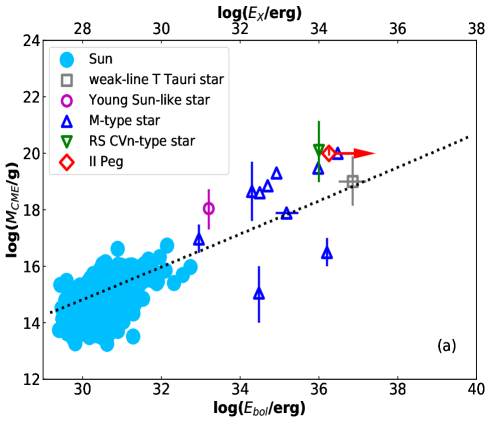
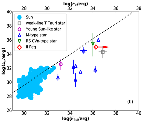
Figure 6: (a) CME mass $M_{CME}$ and (b) kinetic energy $E_{k}$ are plotted as functions of flaring bolometric energy (bottom horizontal axis) and X-ray energy emitted in the GOES band (top axis). The flare energy of II Peg is the lower limit, which therefore is indicated by an arrow in the direction of getting larger. The Solar events are derived from Yashiro & Gopalswamy (2009) and indicated by filled sky-blue circles. The trend fits to the solar data obtained in Drake et al. (2013) are presented by the dotted lines, which could be expressed as $M_{CME}$ $\propto$ $E^{0.59}$ and $E_{k}$ $\propto$ $E^{1.05}$, respectively. Stellar CME candidates on different type stars are obtained from Moschou et al. (2019), Wang et al. (2021, 2022), Namekata et al. (2021), and Inoue et al. (2023).

To compare the detected CME with other events, we convert the flare energy emitted in the H_α line to the GOES X-ray (1–8 Å band) using the scaling relation between H_α and GOES soft X-ray flare energies in Figure 2 and Equation (1) of Haisch (1989), and then use a correction of $E_{bol}$ = 100$E_{X}$ to obtain the bolometric flare energy. Therefore, the lower limit of the bolometric flare energy, $E_{bol}(H_{\alpha})$, is estimated to be 1.8 $\times~{}10^{36}$ erg. Moreover, with the estimated mass and the corresponding velocity, the kinetic energy of CME is inferred to be about 0.76–1.15 $\times~{}10^{35}$ erg during our observation.

We plot the CME mass and kinetic energy as functions of flare energy emitted in the GOES X-ray and bolometric flare energy in Figure 6, which also includes (1) solar CME events studied in Yashiro & Gopalswamy (2009), (2) stellar CME candidates detected by using Doppler shift method and gathered by Moschou et al. (2019) in the literature, (3) possible flare-associated CME candidates on M-dwarf stars (Wang et al., 2021, 2022), (4) an eruptive filament event on a young solar-type star EK Dra (Namekata et al., 2021), (5) a high-velocity prominence eruption leading to a flare-associated CME on the RS CVn-type star V1355 Orionis (Inoue et al., 2023). For EK Dra and V1355 Orionis, the flare energies in GOES X-ray band are also obtained by using the energies emitted in H_α and the scaling relation of Haisch (1989) by us.

It can be seen from the figure that our estimated mass is slightly larger than the value predicted from the solar flare-CME extrapolation, which is similar to the result of RS CVn-type star V1355 Orionis. Taking into account the fact that the flare energy of II Peg is the low limit, we can not say that our estimated mass is inconsistent with the scaling relation of solar events. Moreover, similar to several CME candidates on other active stars, the obtained CME kinetic energy is less than the one extrapolated from solar events. This mainly because the prominence eruptions in stars generally have a much smaller velocity than CMEs on the Sun (Maehara et al., 2021; Namekata et al., 2021). Furthermore, a suppression mechanism by the the overlying magnetic field in active stars is proposed to explain small kinetic energies (e.g., Drake et al., 2016; Alvarado-Gómez et al., 2018). Finally, it is possible that the velocity of stellar CME is greatly underestimated, because it is just the projection component along the line of sight.

4.3 H_α profile asymmetry in the cases without the flares

II Peg is a very active RS CVn-type star with variable H_α emission above the continuum. After using the synthesized spectral subtraction technique, the subtracted H_α profile presents broad wings. When no strong flares happened, it is worth to notice that the broad emission component is always blueshifted (see Table A1 and Fig 3). Broad emission wings had been observed in II Peg (Montes et al., 1997) and in several other chromospheric active stars (e.g. Gu et al., 2002; Montes et al., 1997, 2000; Cao & Gu, 2015). Montes et al. (1998) analyzed the H_α line profile, using the spectral subtraction technique, for chromospherically active binary systems and weak-lined T Tauri stars. They found that, in some active stars, the subtracted H_α line profile has broad wings, which could be interpreted as arising from microflare activity through contrasting with the broad components in the transition region lines.

From Fig 3, it can be seen that there is a close correlation between the contribution of the broad component and the level of stellar activity. That is, the EW variation of the subtracted H_α line is mainly dominated by the broad emission component. On the other hand, there is also a close correlation between the blueshifted velocity of the broad component and the EW. The more blue the broad emission component shifts to, the weaker the EW becomes.

5 Summary and conclusions

Based on the analysis of high-resolution spectroscopic observation of the very active RS CVn-type star II Peg, performed from 2016 January 22 to 31, some interesting results are obtained. Two strong optical flare events were detected on 2016 January 23 and 31, which are demonstrated by the prominent He i D₃ and He i $\lambda$6678 line emission together with the great enhancements in other chromospheric activity lines. The low limits of the flare energies are estimated to be of the order of $10^{33}$ erg and $10^{34}$ erg, respectively, and have reached the scale of stellar superflare. Based on the results of mean spectrum subtraction during the flares, the H_α residual profile shows red asymmetry, whose behavior has a close relation to flaring activity. From what is known about solar flares, chromospheric condensation or coronal rain is a possible origination of the redshifted broad emission components having a velocity of tens of kilometers per second. Most notably, during the second flare, a far-redshifted extra emission component was detected in the H_α line profile and can be explained as caused by a possible stellar prominence eruption. Its Doppler velocity greatly exceeds the star’s escape velocity, which implies that this prominence eruption can develop into a CME event. The mass and kinetic energy of the CME are estimated to be 0.83–1.48 $\times~{}10^{20}$ g and 0.76–1.15 $\times~{}10^{35}$ erg, respectively. The mass is slightly larger than the value expected from the solar flare-CME extrapolation. Similar to several CME candidates on other active stars, the kinetic energy is less than the extrapolated one. In addition, we could not completely rule out the possibility of chromospheric condensation resulting in the far-redshifted extra emission. Finally, when no strong flares happened, there is a blueshifted broad emission component in the STARMOD subtracted H_α line profile. Its behavior is closely associated with the H_α activity features.

Appendix A Measurements for the subtracted chromospheric activity indicators

Table A1 lists the measurements of the subtracted profiles and the fittings of the broad and narrow component of the subtracted H_α line profiles.

Table A1: Measurements of the Subtracted Profiles

HJD	Phase	EW(Å)							$v$(Hαb)	FWHM(Hαb)	$\frac{\bf{EW(\lambda 8542)}}{\bf{EW(\lambda 8498)}}$	$\frac{\bf{E_{H{\alpha}}}}{\bf{E_{H{\beta}}}}$
(2,450,000+)		Ca ii $\lambda 8662$	Ca ii $\lambda 8542$	Ca ii $\lambda 8498$	Hα	Hαn	Hαb	Hβ	(km s-1)	(km s-1)
7409.944	0.259	1.174$\pm$0.001	1.403$\pm$0.024	0.961$\pm$0.036	2.368$\pm$0.077	1.671	0.736	0.807$\pm$0.122	-51.33$\pm$3.96	167.29$\pm$5.70	1.46	4.13
7409.968	0.262	1.193$\pm$0.003	1.377$\pm$0.022	0.952$\pm$0.042	2.254$\pm$0.107	1.577	0.731	0.680$\pm$0.029	-44.07$\pm$3.71	149.81$\pm$5.18	1.45	4.66
7410.943	0.407	1.435$\pm$0.005	1.646$\pm$0.015	1.128$\pm$0.042	3.438$\pm$0.014	1.691	1.754	1.217$\pm$0.161	-2.48$\pm$1.11	184.00$\pm$3.60	1.46	3.97
7410.966	0.410	1.377$\pm$0.001	1.575$\pm$0.012	1.119$\pm$0.060	3.371$\pm$0.002	1.701	1.671	1.074$\pm$0.156	-5.15$\pm$1.15	198.74$\pm$3.55	1.41	4.41
7411.949	0.557	1.191$\pm$0.002	1.398$\pm$0.012	1.010$\pm$0.043	2.543$\pm$0.002	1.373	1.169	0.651$\pm$0.061	-30.03$\pm$1.42	223.67$\pm$3.41	1.38	5.49
7411.972	0.560	1.191$\pm$0.005	1.387$\pm$0.011	1.009$\pm$0.054	2.402$\pm$0.026	1.360	1.055	0.540$\pm$0.020	-29.31$\pm$1.72	210.92$\pm$4.04	1.37	6.26
7412.935	0.703	1.192$\pm$0.009	1.379$\pm$0.019	0.974$\pm$0.058	2.401$\pm$0.001	1.438	0.963	0.673$\pm$0.051	-22.58$\pm$1.11	222.14$\pm$2.91	1.42	5.02
7412.992	0.712	1.182$\pm$0.010	1.362$\pm$0.014	0.972$\pm$0.063	2.549$\pm$0.004	1.417	1.133	0.668$\pm$0.061	-16.26$\pm$1.12	230.58$\pm$3.16	1.40	5.37
7414.931	0.000	1.079$\pm$0.002	1.278$\pm$0.014	0.926$\pm$0.045	2.349$\pm$0.046	1.435	0.937	0.588$\pm$0.042	-34.89$\pm$1.21	178.37$\pm$2.27	1.38	5.62
7415.016	0.013	1.064$\pm$0.001	1.265$\pm$0.016	0.929$\pm$0.054	2.405$\pm$0.028	1.456	0.964	0.565$\pm$0.016	-37.66$\pm$1.45	188.40$\pm$2.75	1.36	5.99
7415.937	0.150	1.185$\pm$0.003	1.413$\pm$0.021	1.004$\pm$0.058	2.736$\pm$0.020	1.449	1.297	0.799$\pm$0.069	-23.83$\pm$0.81	166.11$\pm$1.92	1.41	4.82
7416.012	0.161	1.211$\pm$0.004	1.421$\pm$0.018	1.029$\pm$0.064	2.745$\pm$0.026	1.463	1.295	0.728$\pm$0.017	-20.11$\pm$0.87	161.36$\pm$2.23	1.38	5.30
7416.939	0.299	1.249$\pm$0.009	1.433$\pm$0.016	1.030$\pm$0.065	2.837$\pm$0.020	1.740	1.107	0.736$\pm$0.030	-31.95$\pm$1.32	181.80$\pm$2.62	1.39	5.42
7416.962	0.302	1.257$\pm$0.010	1.437$\pm$0.013	1.025$\pm$0.055	2.807$\pm$0.035	1.687	1.138	0.757$\pm$0.050	-31.46$\pm$1.38	177.39$\pm$2.68	1.40	5.22
7417.971	0.452	1.163$\pm$0.006	1.375$\pm$0.016	0.989$\pm$0.074	1.847$\pm$0.076	1.311	0.574	0.469$\pm$0.017	-66.82$\pm$3.74	152.54$\pm$5.38	1.39	5.54
7417.995	0.456	1.175$\pm$0.008	1.357$\pm$0.018	0.990$\pm$0.075	1.836$\pm$0.089	1.342	0.538	0.475$\pm$0.007	-75.26$\pm$3.98	150.25$\pm$6.03	1.37	5.43
7418.941	0.597	1.662$\pm$0.004	1.986$\pm$0.020	1.342$\pm$0.079	7.895$\pm$0.066	2.262	5.255	2.804$\pm$0.014	31.76$\pm$0.66	307.25$\pm$1.88	1.48	3.96
7418.985	0.603	1.578$\pm$0.002	1.897$\pm$0.018	1.296$\pm$0.064	7.759$\pm$0.037	2.185	5.083	2.367$\pm$0.015	31.45$\pm$1.13	281.71$\pm$2.40	1.46	4.61
7419.012	0.607	1.555$\pm$0.003	1.854$\pm$0.019	1.284$\pm$0.072	7.440$\pm$0.024	2.058	4.861	2.368$\pm$0.010	31.12$\pm$1.35	271.29$\pm$2.57	1.44	4.42

Note. — H_αn and H_αb represent the narrow and broad components of the H_α line, respectively.

References

- Aarnio et al. (2012) Aarnio, A. N., Matt, S. P., & Stassun, K. G. 2012, ApJ, 760, 9, doi: 10.1088/0004-637X/760/1/9
- Airapetian et al. (2016) Airapetian, V. S., Glocer, A., Gronoff, G., Hébrard, E., & Danchi, W. 2016, Nature Geoscience, 9, 452, doi: 10.1038/ngeo2719
- Alvarado-Gómez et al. (2018) Alvarado-Gómez, J. D., Drake, J. J., Cohen, O., Moschou, S. P., & Garraffo, C. 2018, ApJ, 862, 93, doi: 10.3847/1538-4357/aacb7f
- Antolin (2020) Antolin, P. 2020, Plasma Physics and Controlled Fusion, 62, 014016, doi: 10.1088/1361-6587/ab5406
- Antolin et al. (2012) Antolin, P., Vissers, G., & Rouppe van der Voort, L. 2012, Sol. Phys., 280, 457, doi: 10.1007/s11207-012-9979-7
- Argiroffi et al. (2019) Argiroffi, C., Reale, F., Drake, J. J., et al. 2019, Nature Astronomy, 3, 742, doi: 10.1038/s41550-019-0781-4
- Barden (1985) Barden, S. C. 1985, ApJ, 295, 162, doi: 10.1086/163361
- Berdyugina et al. (1999) Berdyugina, S. V., Ilyin, I., & Tuominen, I. 1999, A&A, 349, 863
- Berdyugina et al. (1998) Berdyugina, S. V., Jankov, S., Ilyin, I., Tuominen, I., & Fekel, F. C. 1998, A&A, 334, 863
- Butler et al. (1988) Butler, C. J., Rodono, M., & Foing, B. H. 1988, A&A, 206, L1
- Byrne et al. (1989) Byrne, P. B., Panagi, P., Doyle, J. G., et al. 1989, A&A, 214, 227
- Cao & Gu (2015) Cao, D., & Gu, S. 2015, MNRAS, 449, 1380, doi: 10.1093/mnras/stv110
- Cao et al. (2022) Cao, D., Gu, S., Grundahl, F., & Pallé, P. L. 2022, MNRAS, 514, 4190, doi: 10.1093/mnras/stac1576
- Cao et al. (2020) Cao, D., Gu, S., Wolter, U., Mittag, M., & Schmitt, J. H. M. M. 2020, AJ, 159, 292, doi: 10.3847/1538-3881/ab8f90
- Cao et al. (2023) Cao, D., Gu, S., Wolter, U., et al. 2023, MNRAS, 523, 4146, doi: 10.1093/mnras/stad1700
- Cao et al. (2019) Cao, D., Gu, S., Ge, J., et al. 2019, MNRAS, 482, 988, doi: 10.1093/mnras/sty2768
- Cao & Gu (2017) Cao, D.-T., & Gu, S.-H. 2017, RAA, 17, 055, doi: 10.1088/1674-4527/17/6/55
- Catalano & Frasca (1994) Catalano, S., & Frasca, A. 1994, A&A, 287, 575
- Cherenkov et al. (2017) Cherenkov, A., Bisikalo, D., Fossati, L., & Möstl, C. 2017, ApJ, 846, 31, doi: 10.3847/1538-4357/aa82b2
- Collier Cameron & Robinson (1989) Collier Cameron, A., & Robinson, R. D. 1989, MNRAS, 236, 57, doi: 10.1093/mnras/236.1.57
- Doyle et al. (1991) Doyle, J. G., Kellett, B. J., Byrne, P. B., et al. 1991, MNRAS, 248, 503, doi: 10.1093/mnras/248.3.503
- Drake et al. (2016) Drake, J. J., Cohen, O., Garraffo, C., & Kashyap, V. 2016, in Solar and Stellar Flares and their Effects on Planets, ed. A. G. Kosovichev, S. L. Hawley, & P. Heinzel, Vol. 320, 196–201, doi: 10.1017/S1743921316000260
- Drake et al. (2013) Drake, J. J., Cohen, O., Yashiro, S., & Gopalswamy, N. 2013, ApJ, 764, 170, doi: 10.1088/0004-637X/764/2/170
- Ercolano et al. (2008) Ercolano, B., Drake, J. J., Reale, F., Testa, P., & Miller, J. M. 2008, ApJ, 688, 1315, doi: 10.1086/591934
- Fan et al. (2016) Fan, Z., Wang, H., Jiang, X., et al. 2016, PASP, 128, 115005, doi: 10.1088/1538-3873/128/969/115005
- Favata & Schmitt (1999) Favata, F., & Schmitt, J. H. M. M. 1999, A&A, 350, 900
- Fekel et al. (1986) Fekel, F. C., Moffett, T. J., & Henry, G. W. 1986, ApJS, 60, 551, doi: 10.1086/191097
- Frasca et al. (2008) Frasca, A., Biazzo, K., Taş, G., Evren, S., & Lanzafame, A. C. 2008, A&A, 479, 557, doi: 10.1051/0004-6361:20077915
- Gaia Collaboration (2020) Gaia Collaboration. 2020, VizieR Online Data Catalog, I/350, doi: 10.26093/cds/vizier.1350
- García-Alvarez et al. (2003) García-Alvarez, D., Foing, B. H., Montes, D., et al. 2003, A&A, 397, 285, doi: 10.1051/0004-6361:20021481
- Gu et al. (2002) Gu, S. H., Tan, H. S., Shan, H. G., & Zhang, F. H. 2002, A&A, 388, 889, doi: 10.1051/0004-6361:20020561
- Gu et al. (2003) Gu, S. H., Tan, H. S., Wang, X. B., & Shan, H. G. 2003, A&A, 405, 763, doi: 10.1051/0004-6361:20030671
- Hackman et al. (2012) Hackman, T., Mantere, M. J., Lindborg, M., et al. 2012, A&A, 538, A126, doi: 10.1051/0004-6361/201117603
- Haisch (1989) Haisch, B. M. 1989, A&A, 219, 317
- Hall (1976) Hall, D. S. 1976, in Astrophysics and Space Science Library, Vol. 60, IAU Colloq. 29: Multiple Periodic Variable Stars, ed. W. S. Fitch, 287, doi: 10.1007/978-94-010-1175-4_15
- Hall (1996) Hall, J. C. 1996, PASP, 108, 313, doi: 10.1086/133724
- Hall et al. (1990) Hall, J. C., Huenemoerder, D. P., Ramsey, L. W., & Buzasi, D. L. 1990, ApJ, 358, 610, doi: 10.1086/169013
- Hall & Ramsey (1992) Hall, J. C., & Ramsey, L. W. 1992, AJ, 104, 1942, doi: 10.1086/116370
- Hazra et al. (2022) Hazra, G., Vidotto, A. A., Carolan, S., Villarreal D’Angelo, C., & Manchester, W. 2022, MNRAS, 509, 5858, doi: 10.1093/mnras/stab3271
- Houdebine et al. (1990) Houdebine, E. R., Foing, B. H., & Rodono, M. 1990, A&A, 238, 249
- Huenemoerder & Ramsey (1987) Huenemoerder, D. P., & Ramsey, L. W. 1987, ApJ, 319, 392, doi: 10.1086/165463
- Ichimoto & Kurokawa (1984) Ichimoto, K., & Kurokawa, H. 1984, Sol. Phys., 93, 105, doi: 10.1007/BF00156656
- Inoue et al. (2023) Inoue, S., Maehara, H., Notsu, Y., et al. 2023, ApJ, 948, 9, doi: 10.3847/1538-4357/acb7e8
- Kochukhov et al. (2013) Kochukhov, O., Mantere, M. J., Hackman, T., & Ilyin, I. 2013, A&A, 550, A84, doi: 10.1051/0004-6361/201220432
- Koller et al. (2021) Koller, F., Leitzinger, M., Temmer, M., et al. 2021, A&A, 646, A34, doi: 10.1051/0004-6361/202039003
- Kowalski et al. (2017) Kowalski, A. F., Allred, J. C., Uitenbroek, H., et al. 2017, ApJ, 837, 125, doi: 10.3847/1538-4357/aa603e
- Lacatus et al. (2017) Lacatus, D. A., Judge, P. G., & Donea, A. 2017, ApJ, 842, 15, doi: 10.3847/1538-4357/aa725d
- Leitzinger et al. (2014) Leitzinger, M., Odert, P., Greimel, R., et al. 2014, MNRAS, 443, 898, doi: 10.1093/mnras/stu1161
- Leitzinger et al. (2011) Leitzinger, M., Odert, P., Ribas, I., et al. 2011, A&A, 536, A62, doi: 10.1051/0004-6361/201015985
- Lindborg et al. (2011) Lindborg, M., Korpi, M. J., Hackman, T., et al. 2011, A&A, 526, A44, doi: 10.1051/0004-6361/201015203
- Lindborg et al. (2013) Lindborg, M., Mantere, M. J., Olspert, N., et al. 2013, A&A, 559, A97, doi: 10.1051/0004-6361/201321695
- Longcope (2014) Longcope, D. W. 2014, ApJ, 795, 10, doi: 10.1088/0004-637X/795/1/10
- Maehara et al. (2021) Maehara, H., Notsu, Y., Namekata, K., et al. 2021, PASJ, 73, 44, doi: 10.1093/pasj/psaa098
- Martínez Oliveros et al. (2014) Martínez Oliveros, J.-C., Krucker, S., Hudson, H. S., et al. 2014, ApJ, 780, L28, doi: 10.1088/2041-8205/780/2/L28
- Messina (2008) Messina, S. 2008, A&A, 480, 495, doi: 10.1051/0004-6361:20078932
- Montes et al. (2000) Montes, D., Fernández-Figueroa, M. J., De Castro, E., et al. 2000, A&AS, 146, 103, doi: 10.1051/aas:2000359
- Montes et al. (1998) Montes, D., Fernandez-Figueroa, M. J., de Castro, E., et al. 1998, in Astronomical Society of the Pacific Conference Series, Vol. 154, Cool Stars, Stellar Systems, and the Sun, ed. R. A. Donahue & J. A. Bookbinder, 1516
- Montes et al. (1997) Montes, D., Fernandez-Figueroa, M. J., de Castro, E., & Sanz-Forcada, J. 1997, A&AS, 125, 263, doi: 10.1051/aas:1997374
- Montes et al. (1999) Montes, D., Saar, S. H., Collier Cameron, A., & Unruh, Y. C. 1999, MNRAS, 305, 45, doi: 10.1046/j.1365-8711.1999.02373.x
- Montes et al. (1996) Montes, D., Sanz-Forcada, J., Fernandez-Figueroa, M. J., & Lorente, R. 1996, A&A, 310, L29, doi: 10.48550/arXiv.astro-ph/9604170
- Moschou et al. (2017) Moschou, S.-P., Drake, J. J., Cohen, O., Alvarado-Gomez, J. D., & Garraffo, C. 2017, ApJ, 850, 191, doi: 10.3847/1538-4357/aa9520
- Moschou et al. (2019) Moschou, S.-P., Drake, J. J., Cohen, O., et al. 2019, ApJ, 877, 105, doi: 10.3847/1538-4357/ab1b37
- Namekata et al. (2020) Namekata, K., Maehara, H., Sasaki, R., et al. 2020, PASJ, 72, 68, doi: 10.1093/pasj/psaa051
- Namekata et al. (2021) Namekata, K., Maehara, H., Honda, S., et al. 2021, Nature Astronomy, 6, 241, doi: 10.1038/s41550-021-01532-8
- Namekata et al. (2023) Namekata, K., Airapetian, V. S., Petit, P., et al. 2023, arXiv e-prints, arXiv:2311.07380, doi: 10.48550/arXiv.2311.07380
- Namizaki et al. (2023) Namizaki, K., Namekata, K., Maehara, H., et al. 2023, ApJ, 945, 61, doi: 10.3847/1538-4357/acb928
- Osten & Wolk (2015) Osten, R. A., & Wolk, S. J. 2015, ApJ, 809, 79, doi: 10.1088/0004-637X/809/1/79
- Rodono et al. (1987) Rodono, M., Byrne, P. B., Neff, J. E., et al. 1987, A&A, 176, 267
- Rosén et al. (2015) Rosén, L., Kochukhov, O., & Wade, G. A. 2015, ApJ, 805, 169, doi: 10.1088/0004-637X/805/2/169
- Schrijver & Zwaan (2000) Schrijver, C. J., & Zwaan, C. 2000, Cambridge Astrophysics Series, 34
- Siwak et al. (2010) Siwak, M., Rucinski, S. M., Matthews, J. M., et al. 2010, MNRAS, 408, 314, doi: 10.1111/j.1365-2966.2010.17109.x
- Strassmeier et al. (2019) Strassmeier, K. G., Carroll, T. A., & Ilyin, I. V. 2019, A&A, 625, A27, doi: 10.1051/0004-6361/201834906
- Strassmeier et al. (1993) Strassmeier, K. G., Hall, D. S., Fekel, F. C., & Scheck, M. 1993, A&AS, 100, 173
- Tsuboi et al. (2016) Tsuboi, Y., Yamazaki, K., Sugawara, Y., et al. 2016, PASJ, 68, 90, doi: 10.1093/pasj/psw081
- Veronig et al. (2021) Veronig, A. M., Odert, P., Leitzinger, M., et al. 2021, Nature Astronomy, 5, 697, doi: 10.1038/s41550-021-01345-9
- Vogt (1981) Vogt, S. S. 1981, ApJ, 247, 975, doi: 10.1086/159107
- Wang et al. (2021) Wang, J., Xin, L. P., Li, H. L., et al. 2021, ApJ, 916, 92, doi: 10.3847/1538-4357/ac096f
- Wang et al. (2022) Wang, J., Li, H. L., Xin, L. P., et al. 2022, ApJ, 934, 98, doi: 10.3847/1538-4357/ac7a35
- Wiese & Fuhr (2009) Wiese, W. L., & Fuhr, J. R. 2009, Journal of Physical and Chemical Reference Data, 38, 1129, doi: 10.1063/1.3254213
- Wu et al. (2022) Wu, Y., Chen, H., Tian, H., et al. 2022, ApJ, 928, 180, doi: 10.3847/1538-4357/ac5897
- Xiang et al. (2014) Xiang, Y., Gu, S.-h., Collier Cameron, A., & Barnes, J. R. 2014, MNRAS, 438, 2307, doi: 10.1093/mnras/stt2345
- Yashiro & Gopalswamy (2009) Yashiro, S., & Gopalswamy, N. 2009, in Universal Heliophysical Processes, ed. N. Gopalswamy & D. F. Webb, Vol. 257, 233–243, doi: 10.1017/S1743921309029342
- Zirin (1988) Zirin, H. 1988, Astrophysics of the sun (Cambridge Univ. Press, Cambridge)