Sparse Probabilistic Synthesis of Quantum Operations
Abstract
Successful implementations of quantum technologies require protocols and algorithms that use as few quantum resources as possible. Many applications require a desired quantum operation, such as rotation gates in quantum computing or broadband pulses in NMR or MRI applications, that is not feasible to directly implement or would require longer coherence times than achievable. This work develops an approach that enables—at the cost of a modestly increased measurement repetition rate—the exact implementation of such operations. One proceeds by first building a library of a large number of different approximations to the desired gate operation; by randomly selecting these operations according to a pre-optimised probability distribution, one can on average implement the desired operation with a rigorously controllable approximation error. The approach relies on sophisticated tools from convex optimisation to efficiently find optimal probability distributions. A diverse spectrum of applications are demonstrated as (a) exactly synthesising rotations in fault-tolerant quantum computers using only short T-depth circuits and (b) synthesising broadband and band-selective pulses of superior performance in quantum optimal control with (c) further applications in NMR or MRI. The approach is very general and a broad spectrum of practical applications in quantum technologies are explicitly demonstrated.
I Introduction
With the dawn of quantum computing [1, 2, 3, 4, 5, 6] and other advanced quantum technologies [7], the central experimental/engineering task remains to increase coherence times. It is, however, equally important to find new theoretical tools and protocols that reduce the required quantum resources, such as reducing stringent coherence-time requirements [8, 9, 10, 11, 12, 13].
Here we develop an approach that allows us to implement an ideal, desired quantum operation that is a central resource in quantum technologies but would otherwise not be possible to directly implement, e.g., due to T-depth limitations in quantum computing, finite rotation-angle resolution in quantum simulators or due to finite offset effects in quantum optimum control, quantum metrology, NMR or MRI applications. The present approach overcomes these limitations by approximating the ideal operation as a linear combination of a large number of operations that the hardware can natively implement. We start with an offline pre-processing step whereby we carefully construct a library of gate operations and efficiently find a sparse quasiprobability decomposition through the use of established tools in convex optimisation. The online, experimental implementation then proceeds by randomly choosing the operations according to probabilities determined by . This protocol can on average implement the desired quantum operation through a rigorously controllable, arbitrarily small approximation error.
The present approach resembles to certain quantum error mitigation techniques which, however, address a distinct problem as they mitigate the effect of hardware imperfections [14, 15]. In fact, we will first assume gate operations to be noise-free – while we discuss below that indeed the approach can naturally be combined with quantum error mitigation protocols. Furthermore, Probabilistic Error Cancellation [16, 17, 18] typically applies Clifford recovery operations which would be many orders of magnitude less efficient in the present context as we demonstrate below. In contrast, the present approach uses a large number of operations that are close to the desired operation – this however, makes our classical pre-processing step rather challenging as it requires manipulating ill-conditioned design matrices and thus standard tools from convex optimisation are impractical. For example, we will consider sequences of Clifford and T gates that approximate the same continuous rotation, and are thus very close to each other resulting in an ill-conditioned optimisation problem.
We address this technical challenge by first posing the decomposition as the solution of an underdetermined linear system of equations. Given underdetermined equations may have infinitely many solutions, our aim is to find the optimal one that has a minimal norm and thus guarantees a minimal measurement overhead of the approach. In fact, an important result in the theory of linear systems is that the minimal L1-norm solution is almost always the sparsest [19, 20] – finding such sparse solutions has become a very well explored and understood field in mathematics with numerous important applications in engineering, signal processing (compressed sensing) and in machine learning [19, 20]. We employ sophisticated Least Angle Regression (LARS) solvers [19, 21] that can achieve arbitrary precision while allowing us to efficiently prepare not only the exact solution but an entire, continuous family of solutions that make a tradeoff between approximation error and L1 norm (measurement overhead).
We demonstrate a diverse spectrum of practical applications in quantum technologies. First, we demonstrate the exact synthesis of continuous-angle rotations in fault-tolerant quantum computers using only short T-depth sequences such that the measurement overhead achieved is more than 4 orders of magnitude lower than with previous techniques. Second, we demonstrate how the present approach enables exactly or approximately synthesising broadband and band-selective pulses in quantum optimum control – which can ultimately lower error rates due to finite-bandwidth effects in native, physical quantum gates used in today’s quantum computers and quantum simulators. Third, we extend these results to NMR and MRI applications where broadband and band-selective pulses are crucial [22]. Finally, we considerably expand prior results on overcoming finite rotation-angle resolution due to discretisation in the classical control electronics.
This manuscript is organised as follows. In Section II we first review the basic theory of probabilistic schemes that use quasiprobability decompositions. We then pose the present problem as solving an underdetermined system of equations, introduce convex optimisation and the numerical solvers one can employ. In Section III we detail a broad range of practical applications with explicit examples.
II Theory
II.1 Quasiprobability representations
In the following we refer to a unitary operator in terms of its process matrix (which acts on a vectorised density matrix isomorphically with conjugation as ). To simplify our presentation, we further assume that is the Pauli transfer matrix such that is a real matrix [23]. Due to the exponential dimensionality of the process matrices the approach is limited to only few-qubit operations, however, this is sufficient in most practical applications given quantum circuits are typically built of local gate operations (1 qubit and 2 qubit operations).
The central aim of this work is to implement a desired, high-cost gate operation (e.g., one that the hardware can only implement at a substantial quantum overhead) as a linear combination of gates that the quantum hardware can natively implement at low cost as
| (1) |
For example, we will consider applications where would require an infinitely long sequence of Clifford and gates whereas are finite-depth approximations. While the decomposition in Eq. 1 cannot be directly realised in an experiment, it can be implemented as the average of the following random sampling scheme [24].
Statement 1.
We define a sampling scheme that implements on average by randomly choosing the gates in our library according to the probability distribution . Then we obtain an unbiased estimator of the desired quantum gate as
| (2) |
with the property .
Refer to Section B.1 for a proof. Similar sampling schemes have been employed in the context of quantum error mitigation whereby the approach is typically called a quasiprobability representation [17, 16, 25] due to the possibly negative coefficients ; While it is not possible to directly inflict the negative weight in a single experiment, one uses the above scheme to estimate expectation values whereby individual measurement outcomes are multiplied in post-processing with the sign of the relevant circuit variant. Negative signs then cause an increase in variance and thus an increased number of circuit repetitions are required for estimating an observable via the L1 norm .
Statement 2.
Applying 1 to the estimation of the expected value of an observable results in the unbiased estimator such that . The number of shots required to achieve precision is upper bounded (assuming norm ) as . Building a quantum circuit of probabilistic gate implementations results in the overhead as
| (3) |
where is the largest norm – and of course the circuit can additionally contain any number of deterministically chosen gates.
Refer to Section B.2 for a proof that explicitly constructs the estimator . The above measurement cost is exponentially larger than having direct access to in which case a constant number of shots would suffice. Still, the present approach is highly beneficial in practice as long as the number of gates in the circuit is not significantly larger than – and indeed the present bounds are quite pessimistic and the actual overhead may be orders of magnitude lower [24, 26].
Our primary aim is to find decompositions which have an overhead as low as possible – we achieve this via two conceptually different routes. First, we carefully design a library of gates (design matrix) which by construction provides low overhead solutions. Second, out of the infinite family of solutions we choose the unique one that minimises the L1 norm of the solution vector.
II.2 Constructing a design matrix
We start by vectorising all process matrices and by stacking column vectors on top of each other; We then arrange these (column) vectors into a design matrix as
| (4) |
where on the right-hand side we re-write Eq. 1 as a matrix-vector equation. The above is a linear system of equations with an unknown vector and a design matrix of dimension .
We detail in the Appendix that quantum error mitigation [27] protocols mostly consider square design matrices R of dimension that are well-conditioned and invertible [16, 27], e.g., a single-qubit gate is mitigated using 16 Clifford operations through the unique solution . Unfortunately, mitigating coherent errors using Clifford operations may result in many orders of magnitude larger overheads than an optimal scheme with minimal overhead: ref [24] analytically proved that a minimal L1 norm is achieved when quantum operations are chosen that are as close to the desired operation as possible – in addition to possible Clifford operations.
In the present case we aim to find low-overhead solutions by constructing our design matrix of a large number of operations that are as close to the desired one as possible. We will thus assume that the column dimension of R is smaller than its row dimension via and typically R is ill-conditioned.
II.3 Convex optimisation
Given a fixed design matrix as outlined in the previous section, the system of equations in Eq. 4 is underdetermined and thus may have infinitely many solutions; our aim is thus to find the unique solution with minimal L1 norm as
| (5) |
Such minimal l1-norm solutions are a) almost always the sparsest solutions and b) can be solved efficiently using tools from convex optimisation [19, 20]. More specifically, we consider the more general optimisation that additionally allows us to find approximate solutions as
| (6) |
By choosing a sufficiently large one demands a sparse but approximate solution while decreasing yields more accurate solutions at the expense of increasing the norm . Solving Eq. 6 has been central to a wide array of practical applications: the problem is known as basis pursuit denoising (BPDN) [28] in signal processing while it is known as LASSO in machine learning applications [29]. As such, a significant advantage compared to, e.g., generic linear programming solvers is that fast, specific solvers are available.
In the present work we specifically construct design matrices that are ill-conditioned which may result in numerical precision issues. For this reason we use a LARS solver that constructs very accurate solutions via the following steps [19, 21]: One starts by solving Eq. 6 in the limit via the null vector . Then the value of is reduced such that a single vector entry is selected that has the highest potential of reducing the error term and a new solution vector is provided with only a single non-zero entry. The approach then adds single entries to the vector gradually reducing the value of until an exact solution is found (or is approached). The significant advantage of this approach is that we construct the entire path along . Thus we can efficiently obtain a solution where the constraint is exactly satisfied, i.e., no overhead, which is very useful in practice as we demonstrate later.
Furthermore, we note that the error term in Eq. 6 is the Hilbert-Schmidt distance between the two process matrices and . Recall that the Hilbert-Schmidt distance of two density matrices is an operationally invariant distance between two fixed quantum states expressing an average distance in terms of measurement probabilities [30]. Similarly, the Hilbert-Schmidt distance between two process matrices expresses the average distance between two quantum processes as detailed in [31].
III Applications
III.1 Application 1: Fault-tolerant gate synthesis
Fault-tolerant quantum computers typically achieve universality through decomposing continuous rotation gates into sequences of (relatively) expensive T-gates and (relatively) cheaper Clifford gates; well-established algorithms are available that efficiently decompose any single-qubit rotation into such sequences [33]. However, in early fault-tolerant quantum computers one will make frugal use of T gates – the limited depth of Clifford+T sequences thus introduces a coherent deviation from the desired quantum operation.
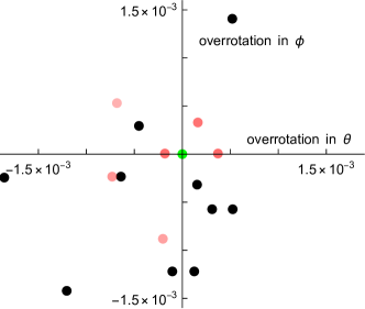
We build on the observation that a large number of Clifford+T sequences can be constructed that contain at most T gates and approximate the ideal gate to a precision at least . For example, we consider a single-qubit rotation and explicitly construct a library of different Clifford+T sequences as that achieve a precision (Hilbert-Schmidt distance) at least using no more than T gates. The design matrix is then obtained by appending a further 15 single-qubit Clifford operations to one of the such that . Fig. 1 (black and red dots) illustrates the overrotation in spherical angles and with respect to the ideal operation (green) when applying elements of the gate library onto an initial quantum state.
By solving the optimisation problem in Eq. 5 for we obtain an exact solution that allows to exactly synthesise the desired Z rotation gate (green dot) at a minimal measurement overhead – this overhead is more than 4 orders of magnitude lower than using Clifford recovery operations only as in [16, 27, 32] in which case . Furthermore, Fig. 1 illustrates that indeed our solution is sparse as most gates in the library receive zero coefficients (black dots, ) while red dots correspond to elements of the library that receive non-zero coefficients while their opacity is proportional to the absolute values of .
III.2 Application 2: Quantum optimum control
Physical quantum gates are typically implemented in hardware by electronically controlling the interaction strength between qubits and external electromagnetic fields. Sophisticated optimum control techniques have been developed for numerically discovering non-trivial control-pulse shapes [34, 35]. Given each instance of the numerical search typically finds a local optimum, we can build a library of these different optimum control solutions ; By solving Eq. 6 we can then either exactly, or approximately but with lower approximation error than any of the , implement the desired gate on average.
To simplify our presentation, let us consider the specific problem of synthesising a single-qubit rotation —while of course the approach applies generally to any other optimum control scenario—via the time-dependent Hamiltonian as
| (7) |
Here the piecewise-constant, complex parameters control the strength of the Pauli and interactions for each timestep and typically correspond to the phase and amplitude of an applied RF or MW pulse. Furthermore, is a drift Hamiltonian, i.e., an interaction that the hardware cannot directly control. Implementing the piecewise constant pulse in which each piece has length yields the unitary gate as
Optimum control techniques numerically optimise the parameters in order to maximise the fidelity of the emerging unitary gate that depends on the drift – broadband pulses then maximise for a broad range of values.
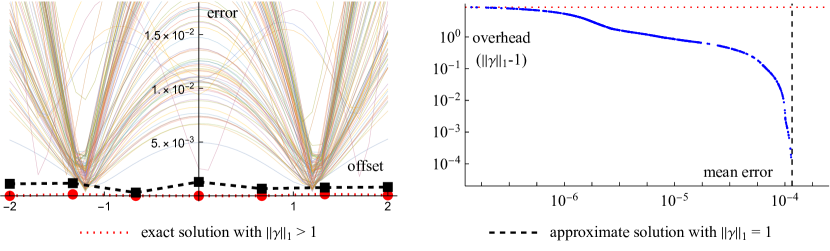
Fig. 2 (left, solid lines) shows approximation errors (Hilbert-Schmidt distance) in a library of shaped pulses that were optimised to achieve maximal fidelity in the range of dimensionless offset values . Exactly achieving an rotation for a broad range of offsets requires arbitrarily large amplitudes , however, in order to limit the energy dissipation of the quantum hardware it is highly desirable to cap the maximum allowed amplitude. The optimised pulses in Fig. 2 (left, solid lines) were capped at and thus the approximation error is non-zero but minimal. Indeed, as each pulse optimisation was initialised in a different random seed, each converged to a different local optimum resulting in a different process matrix and a different error-distribution curve in Fig. 2 (left, solid lines). We build a library of these process matrices and apply our probabilistic approach to exactly implement on average the desired rotation for a range of offset values .
For this reason, we first discretise the offset range into discrete values and stack the corresponding vectorised process matrices on top of each other as
The vectors on the left-hand side then form columns of our design matrix as in Eq. 4. Thus, discretising the offset range into pieces results in a column dimension of the design matrix that has been increased by a factor of . The vector of the desired process (right-hand side of the above equation) then simply consists of copies of the vectorised process matrix of the desired operation. The linear system of equations must have thus solutions that guarantee that the same is obtained for all offset values .
Fig. 2(left, red dots) shows the exact solution for using the design matrix of size that was constructed by discretising the offset range into grid points for different shaped pulses and appending additional Clifford operations (achieved via, e.g., phase shifts of the pulses). As detailed in Section II.3, the solution is constructed by starting at and gradually decreasing the sparsity of the vector which monotonically decreases the error while also monotonically increasing the norm . The resulting trade-off curve is shown in Fig. 2(right) where the approximation error (x axis) is plotted against the L1 norm (y axis) – the L1 norm of the aforementioned exact solution is shown by the dotted red line.
In applications where a lower measurement cost is desired, an approximate solution of small L1 norm may be preferred. Among these, one can obtain a solution that achieves zero measurement overhead via , i.e., Fig. 2(right, dashed black). The average approximation error over the relevant drift values is illustrated in Fig. 2(left, dashed black) which confirms that indeed the approximate solution outperforms any of the individual optimised pulses (lower approximation error than solid lines) even though no measurement overhead is introduced.
A number of natural generalisations and further applications are apparent. For example, following the same steps one can construct band-selective pulses via the vectorised process matrix as
This construction of can be used guarantee that is applied only within the offset range while the identity operation is applied otherwise.
III.3 Application 3: broadband and band-selective pulses in NMR and MRI
The techniques introduced in the previous section naturally extend to NMR and MRI applications, where broadband and band-selective pulses are essential. We illustrate our approach on the specific application where an ideal, rotation needs to be implemented (which is again represented via its Pauli transfer matrix); This gate operation is used to transform the average state of a very large number of nuclear or electron spins as the mixed state as [22]
| (8) |
By convention, the initial state is proportional to the Pauli matrix (ignoring the identity term in that that does not contribute to the measurement outcome [22]). Optimal control techniques can be used to obtain pulses that best approximate the ideal action in order to obtain the transformed state that is proportional to the Pauli matrix.
A simple NMR or MRI experiment then proceeds by allowing this state to freely evolve for time into under the natural Hamiltonian of the spin system; Measuring Pauli and operators yield real and imaginary parts of the classical time-dependent signal as
| (9) |
Finally, the experiment may be repeated times in order to suppress statistical noise in by a factor and the resulting average signal is Fourier transformed to obtain an NMR spectrum. However, as explained in the previous section, the pulses illustrated in Fig. 2 (solid lines) incur an approximation error due the drift term and thus the state is not exactly the desired one .
We can adapt our probabilistic scheme in 1 such that we randomly choose pulses to be implemented in an NMR or MRI experiment.
Statement 3.
Refer to Section B.5 for a proof. The above statement results in the following practical protocol: We first randomly choose a pulse and use it to prepare the initial state via Eq. 8, we measure the signal as a function of the evolution time as in Eq. 9, multiply each signal with the relevant sign and the L1 norm of the solution vector; The mean of the resulting signals is then guaranteed to recover the ideal signal that one would obtain by applying the ideal gate at each offset value , i.e., red dots and black squares in Fig. 2.
As an NMR experiment is repeated times to suppress random noise by a factor , indeed the number of repetitions required to achieve precision scales as just like in the case of quantum computing applications in 2. Furthermore, complex NMR pulse sequences may apply multiple different gate elements one after the other – one would then replace each gate element with the relevant estimators from 3, the same way as quantum circuits are constructed in 2; The measurement overhead then similarly grows exponentially with the number of gate elements.
III.4 Application 4: optimality of Probabilistic Angle Interpolation
Most leading quantum computing platforms require cryogenic cooling which introduces a communication bottleneck – hardware developers thus aim to move control electronics closer to the QPU which, however, introduces limitations to the classical control electronics, such as low-precision discretisation of continuous rotation gates [24]. PAI resolves this issue [24] by effectively implementing a continuous-angle rotation gate when the hardware platform can only implement a discrete set of rotations via the angles as with .
We use the present approach to verify that the analytical solution of ref [24] solves the exact optimisation problem in Eq. 5 and also to obtain further, approximate solutions via the generalised optimisation problem in Eq. 6. In particular, ref [24] obtained an analytical decomposition whereby only 3 gate configurations receive non-zero coefficients , i.e., one randomly chooses one of the two notch settings and nearest to the desired angle as well as a third setting that corresponds to the polar opposite rotation .
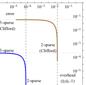
We illustrate our approach by considering a single-qubit Pauli X rotation at discretised rotation angles with bits of precision and build a design matrix of size that contains all discrete gate variants; we find the following conclusions. First, we find that a 3-sparse solution exactly implements the desired gate () and confirm that this solution is identical to the analytical solution of ref. [24]. Second, the significant advantage of the present approach is that we can additionally obtain approximate solutions in Eq. 6 via that have lower measurement cost. As such, we obtain a 2-sparse solution that achieves zero measurement overhead as . Interestingly, this (optimal) solution achieves slightly lower approximation error than a naive solution whereby one chooses with probability and chooses with probability , where is the relative position of the desired angle to the two nearest notch settings.
Third, by linear combining the 2-sparse and 3-sparse solution vectors, we obtain an infinite family of solutions that make a tradeoff between approximation error and measurement overhead (Fig. 3, blue solid). In comparison, using only Clifford recovery operations as in [32] results in orders of magnitude higher measurement overheads and approximation errors (Fig. 3, blue solid).
IV Discussion and conclusion
The present work develops an approach that allows one to synthesise quantum operations that would otherwise be impossible to implement directly in quantum hardware. This is achieved by probabilistically interpolating between nearby quantum operations that can be realised natively by the quantum hardware.
Probabilistic schemes have been used in quantum error mitigation for mitigating gate errors and have also been used to overcome coherent errors in unitary gates. However, previous approaches used Clifford recovery operations which allow for finding decompositions via well-conditioned design matrices. Presently, however, we consider a library of gate operations that are close to each other, e.g., gates or gate sequences that approximate the ideal operation. This guarantees a minimal measurement overhead of the approach, however, makes the numerical pre-processing step challenging as one needs to solve a non-trivial underdetermined system of equations. By using sophisticated tools from convex optimisation we obtain numerically exact, arbitrary-precision solutions. Furthermore, as we demonstrate, the present approach achieves orders of magnitude lower measurement overheads than using Clifford-based techniques in the context of quantum computing. A significant advantage of the present approach is that it is directly compatible with both error mitigation and with advanced, randomised measurement techniques, such as classical shadows [36] (via the approach of [18]) and will thus benefit a broad set of applications [37, 38].
Furthermore, the present approach is very general and can be applied to a broad range of application scenarios beyond quantum computing: we explicitly demonstrate practical applications as synthesising perfect (or approximate) broadband and band-selective pulses in quantum optimum control – as we explicitly demonstrate, these results naturally extend to NMR and MRI applications.
The present work is an important stepping stone in developing advanced quantum protocols whereby the quantum resources are significantly reduced through the use of classical computers that solve non-trivial but offline, classical pre and post processing tasks. While related probabilistic techniques are routinely used in the context of quantum error mitigation, the present work significantly generalises these mathematical concepts to a wide spectrum of entirely new application scenarios in quantum technologies.
Acknowledgments
B.K. thanks the University of Oxford for a Glasstone Research Fellowship and Lady Margaret Hall, Oxford for a Research Fellowship. The numerical modelling involved in this study made use of the Quantum Exact Simulation Toolkit (QuEST), and the recent development QuESTlink [39] which permits the user to use Mathematica as the integrated front end, and pyQuEST [40] which allows access to QuEST from Python. We are grateful to those who have contributed to all of these valuable tools. The authors would like to acknowledge the use of the University of Oxford Advanced Research Computing (ARC) facility [41] in carrying out this work and specifically the facilities made available from the EPSRC QCS Hub grant (agreement No. EP/T001062/1). The author also acknowledges funding from the EPSRC projects Robust and Reliable Quantum Computing (RoaRQ, EP/W032635/1) and Software Enabling Early Quantum Advantage (SEEQA, EP/Y004655/1).
Appendix A Related works
A.1 Quantum error mitigation
Reducing the sampling overhead has been explored in the context of quantum error mitigation (QEM) [27]: the diamond distance was minimised under the constraint that the overhead stay below a threshold – this problem can be solved efficiently using semidefinite programming. Furthermore, as explained in the main text in QEM one typically chooses the design matrix as a well-conditioned, invertible square matrix, e.g., for a single qubit one uses 16 Clifford operations [16, 27], such that Eq. 4 can be solved straightforwardly as .
In the present case we use a large number of gate operations that are very close to each other resulting in a highly ill-conditioned design matrix whose row dimension is larger than its column dimension, i.e., a non-square matrix. For this reason we use the Hilbert-Schmidt distance to quantify discrepancy between operations, rather than the diamond distance of [27], which allows us to pose the present problem as solving an underdetermined system of equations. Posing the problem this way is a key enabler as we can use precise, efficient special-purpose solvers rather than generic SDP solvers – achieving high numerical precision with generic SDP solvers may be difficult.
For this reason we consider applications where one assumes perfect unitary operations and the only source of error is due to, e.g., finite T depth or discretisation of quantum rotation angles etc. Furthermore, operations and are known exactly, hence arbitrary precision numerical representations can be used. This is all in contrast to QME [27] whereby one approximately learns these from experiments and one thus needs to consider low-precision numerical representations.
While in the main text we assumed the gates are noise free, indeed, in a realistic experiment the gate elements are likely not perfect. A natural error mitigation strategy was outlined in [24] that immediately applies to the present approach. In particular, one can efficiently learn the noise model for each gate variant and probabilistically implement noise-free variants using Probabilistic Error Cancellation. Hence, the present approach remains unchanged, except, its measurement cost is increased by a factor due to PEC.
A.2 Probabilistic gate synthesis
Probabilistic gate sequences have been employed to improve the accuracy of Clifford+T sequences [42, 43, 44]. In particular, the desired unitary operation is approximated as where is a probability distribution and are is a set of operations close to but with finite T depth. It was observed that the approximation error in is always quadratically smaller than in . However, these techniques are approximate and as one increases the number of gates in the circuit, the fidelity of the quantum state decreases exponentially as demonstrated in [24].
In contrast, the present approach allows to exactly synthesise through the use of both positive and negative weights in Eq. 1; when the aim is to estimate expected values the sign can be applied in post processing. Furthermore, in contrast to those prior techniques, in our case additionally include polar opposite rotations given these guarantee the minimal measurement overhead [24]. Indeed, as our approach exactly implements the desired gate, it comes with an increased measurement overhead that depends quadratically on the precision, i.e., .
A.3 Cooperative optimum control
It was originally proposed in ref [45] that shaped pulses that implement a desired rotation need not be individually accurate but rather need only satisfy a relaxed condition that the average of a series of pulse variants are required to be accurate over many repeated of measurement rounds. The present approach is indeed quite comparable, however, we allow for the additional freedom that different gate/circuit variants are not simply averaged over but we rather calculate a weighted average where we allow for negative weights even.
Appendix B Proofs
B.1 Proof of 1
Proof.
We can explicitly evaluate the expected value as
and upon substituting we obtain
where in the last equation we used Eq. 1. ∎
B.2 Proof of 2
B.3 Unbiasedness
Proof.
We first start by introducing the measurement of an observable via a set of POVMs admitting the property . The expected value of an observable is obtained via the estimator via the corresponding probability distribution .
B.4 Bounding the number of shots
Proof.
For an unbiased estimator, the variance can be upper bounded as
We thus need only bound the expected value of the square of the estimator as
where in the second equation we used the inequality . Finally, the bound on the variance follows as
Thus the number of samples required to achieve a precision scales as
| (15) |
Adapting the proof technique of Statement 3 in [24], it is straightforward to extend this bound to the case of quantum circuits composed of applications of a quasiprobability decomposition in which case the variance is upper bounded as
| (16) |
where correspond to the individual quasiprobability decompositions and is thus bounded by the largest one , therefore . Thus, the number of samples scales in the worst case as
| (17) |
∎
B.5 Proof of 3
We can prove unbiasednes of the estimator by computing the expected value
| (18) |
Substituting the probability results in
| (19) | ||||
where in the second equation we substituted the definition of from Eq. 9. We can simplify the right-hand side by denoting or as as
Appendix C Details of Fig. 1
We used the grdidsynth package [33] to optimally synthesize Clifford + T sequences that approximate to a precision at least as we described in the main text. 150 digits of precision was needed to achieve machine precision in the solution vector.
Appendix D Details of Fig. 2
The cost function was maximised via a gradient descent optimisation of the pulse amplitudes. The single-qubit transfer matrices needed 400 digits of precision to achieve machine precision in the exact solution.
References
- Arute et al. [2019] F. Arute, K. Arya, R. Babbush, D. Bacon, J. C. Bardin, R. Barends, R. Biswas, S. Boixo, F. G. S. L. Brandao, D. A. Buell, B. Burkett, Y. Chen, Z. Chen, B. Chiaro, R. Collins, W. Courtney, A. Dunsworth, E. Farhi, B. Foxen, A. Fowler, C. Gidney, M. Giustina, R. Graff, K. Guerin, S. Habegger, M. P. Harrigan, M. J. Hartmann, A. Ho, M. Hoffmann, T. Huang, T. S. Humble, S. V. Isakov, E. Jeffrey, Z. Jiang, D. Kafri, K. Kechedzhi, J. Kelly, P. V. Klimov, S. Knysh, A. Korotkov, F. Kostritsa, D. Landhuis, M. Lindmark, E. Lucero, D. Lyakh, S. Mandrà, J. R. McClean, M. McEwen, A. Megrant, X. Mi, K. Michielsen, M. Mohseni, J. Mutus, O. Naaman, M. Neeley, C. Neill, M. Y. Niu, E. Ostby, A. Petukhov, J. C. Platt, C. Quintana, E. G. Rieffel, P. Roushan, N. C. Rubin, D. Sank, K. J. Satzinger, V. Smelyanskiy, K. J. Sung, M. D. Trevithick, A. Vainsencher, B. Villalonga, T. White, Z. J. Yao, P. Yeh, A. Zalcman, H. Neven, and J. M. Martinis, Quantum supremacy using a programmable superconducting processor, Nature 574, 505 (2019).
- Wu et al. [2021] Y. Wu, W.-S. Bao, S. Cao, F. Chen, M.-C. Chen, X. Chen, T.-H. Chung, H. Deng, Y. Du, D. Fan, M. Gong, C. Guo, C. Guo, S. Guo, L. Han, L. Hong, H.-L. Huang, Y.-H. Huo, L. Li, N. Li, S. Li, Y. Li, F. Liang, C. Lin, J. Lin, H. Qian, D. Qiao, H. Rong, H. Su, L. Sun, L. Wang, S. Wang, D. Wu, Y. Xu, K. Yan, W. Yang, Y. Yang, Y. Ye, J. Yin, C. Ying, J. Yu, C. Zha, C. Zhang, H. Zhang, K. Zhang, Y. Zhang, H. Zhao, Y. Zhao, L. Zhou, Q. Zhu, C.-Y. Lu, C.-Z. Peng, X. Zhu, and J.-W. Pan, Strong Quantum Computational Advantage Using a Superconducting Quantum Processor, Physical Review Letters 127, 180501 (2021).
- Zhong et al. [2021] H.-S. Zhong, Y.-H. Deng, J. Qin, H. Wang, M.-C. Chen, L.-C. Peng, Y.-H. Luo, D. Wu, S.-Q. Gong, H. Su, Y. Hu, P. Hu, X.-Y. Yang, W.-J. Zhang, H. Li, Y. Li, X. Jiang, L. Gan, G. Yang, L. You, Z. Wang, L. Li, N.-L. Liu, J. J. Renema, C.-Y. Lu, and J.-W. Pan, Phase-Programmable Gaussian Boson Sampling Using Stimulated Squeezed Light, Physical Review Letters 127, 180502 (2021).
- Bluvstein et al. [2023] D. Bluvstein, S. J. Evered, A. A. Geim, S. H. Li, H. Zhou, T. Manovitz, S. Ebadi, M. Cain, M. Kalinowski, D. Hangleiter, J. P. B. Ataides, N. Maskara, I. Cong, X. Gao, P. S. Rodriguez, T. Karolyshyn, G. Semeghini, M. J. Gullans, M. Greiner, V. Vuletić, and M. D. Lukin, Logical quantum processor based on reconfigurable atom arrays, Nature , 1 (2023).
- Kim et al. [2023] Y. Kim, A. Eddins, S. Anand, K. X. Wei, E. van den Berg, S. Rosenblatt, H. Nayfeh, Y. Wu, M. Zaletel, K. Temme, and A. Kandala, Evidence for the utility of quantum computing before fault tolerance, Nature 618, 500 (2023).
- ach [2023] Suppressing quantum errors by scaling a surface code logical qubit, Nature 614, 676 (2023).
- Acín et al. [2018] A. Acín, I. Bloch, H. Buhrman, T. Calarco, C. Eichler, J. Eisert, D. Esteve, N. Gisin, S. J. Glaser, F. Jelezko, et al., The quantum technologies roadmap: a european community view, New Journal of Physics 20, 080201 (2018).
- Cerezo et al. [2021] M. Cerezo, A. Arrasmith, R. Babbush, S. C. Benjamin, S. Endo, K. Fujii, J. R. McClean, K. Mitarai, X. Yuan, L. Cincio, and P. J. Coles, Variational quantum algorithms, Nature Reviews Physics 3, 625 (2021).
- Endo et al. [2021] S. Endo, Z. Cai, S. C. Benjamin, and X. Yuan, Hybrid Quantum-Classical Algorithms and Quantum Error Mitigation, Journal of the Physical Society of Japan 90, 032001 (2021).
- Bharti et al. [2022] K. Bharti, A. Cervera-Lierta, T. H. Kyaw, T. Haug, S. Alperin-Lea, A. Anand, M. Degroote, H. Heimonen, J. S. Kottmann, T. Menke, W.-K. Mok, S. Sim, L.-C. Kwek, and A. Aspuru-Guzik, Noisy intermediate-scale quantum algorithms, Rev. Mod. Phys. 94, 015004 (2022).
- van Straaten and Koczor [2021] B. van Straaten and B. Koczor, Measurement cost of metric-aware variational quantum algorithms, PRX Quantum 2, 030324 (2021).
- Koczor and Benjamin [2022a] B. Koczor and S. C. Benjamin, Quantum analytic descent, Physical Review Research 4, 023017 (2022a).
- Koczor and Benjamin [2022b] B. Koczor and S. C. Benjamin, Quantum natural gradient generalized to noisy and nonunitary circuits, Phys. Rev. A 106, 062416 (2022b).
- Cai et al. [2022] Z. Cai, R. Babbush, S. C. Benjamin, S. Endo, W. J. Huggins, Y. Li, J. R. McClean, and T. E. O’Brien, Quantum error mitigation, arXiv preprint arXiv:2210.00921 (2022).
- Koczor [2021] B. Koczor, Exponential error suppression for near-term quantum devices, Phys. Rev. X 11, 031057 (2021).
- Endo et al. [2018] S. Endo, S. C. Benjamin, and Y. Li, Practical quantum error mitigation for near-future applications, Phys. Rev. X 8, 031027 (2018).
- Temme et al. [2017] K. Temme, S. Bravyi, and J. M. Gambetta, Error mitigation for short-depth quantum circuits, Phys. Rev. Lett. 119, 180509 (2017).
- Jnane et al. [2024] H. Jnane, J. Steinberg, Z. Cai, H. C. Nguyen, and B. Koczor, Quantum error mitigated classical shadows, PRX Quantum 5, 010324 (2024).
- Elad [2010] M. Elad, Sparse and redundant representations: from theory to applications in signal and image processing, Vol. 2 (Springer, 2010).
- Schmidt et al. [2007] M. Schmidt, G. Fung, and R. Rosales, Fast optimization methods for l1 regularization: A comparative study and two new approaches, in Machine Learning: ECML 2007: 18th European Conference on Machine Learning, Warsaw, Poland, September 17-21, 2007. Proceedings 18 (Springer, 2007) pp. 286–297.
- Loris [2008] I. Loris, L1packv2: A mathematica package for minimizing an l1-penalized functional, Computer physics communications 179, 895 (2008).
- Levitt [2013] M. H. Levitt, Spin dynamics: basics of nuclear magnetic resonance (John Wiley & Sons, 2013).
- Nielsen and Chuang [2010] M. A. Nielsen and I. L. Chuang, Quantum computation and quantum information (Cambridge university press, 2010).
- Koczor et al. [2023] B. Koczor, J. Morton, and S. Benjamin, Probabilistic interpolation of quantum rotation angles, Phys Rev Lett (accepted, in production), arXiv preprint arXiv:2305.19881 (2023).
- Berg et al. [2022] E. v. d. Berg, Z. K. Minev, A. Kandala, and K. Temme, Probabilistic error cancellation with sparse Pauli-Lindblad models on noisy quantum processors, arXiv preprint arXiv:2201.09866 (2022).
- Tran et al. [2023] M. C. Tran, K. Sharma, and K. Temme, Locality and Error Mitigation of Quantum Circuits, arXiv:2303.06496 (2023).
- Piveteau et al. [2022] C. Piveteau, D. Sutter, and S. Woerner, Quasiprobability decompositions with reduced sampling overhead, npj Quantum Information 8, 12 (2022).
- Chen et al. [2001] S. S. Chen, D. L. Donoho, and M. A. Saunders, Atomic decomposition by basis pursuit, SIAM review 43, 129 (2001).
- Simon et al. [2013] N. Simon, J. Friedman, T. Hastie, and R. Tibshirani, A sparse-group lasso, Journal of computational and graphical statistics 22, 231 (2013).
- Lee et al. [2003] J. Lee, M. Kim, and Č. Brukner, Operationally invariant measure of the distance between quantum states by complementary measurements, Physical review letters 91, 087902 (2003).
- Maciejewski et al. [2023] F. B. Maciejewski, Z. Puchała, and M. Oszmaniec, Exploring quantum average-case distances: proofs, properties, and examples, IEEE Transactions on Information Theory (2023).
- Suzuki et al. [2022] Y. Suzuki, S. Endo, K. Fujii, and Y. Tokunaga, Quantum error mitigation as a universal error reduction technique: Applications from the NISQ to the fault-tolerant quantum computing eras, PRX Quantum 3, 010345 (2022).
- Ross and Selinger [2014] N. J. Ross and P. Selinger, Optimal ancilla-free clifford+ t approximation of z-rotations, arXiv preprint arXiv:1403.2975 (2014).
- Werschnik and Gross [2007] J. Werschnik and E. Gross, Quantum optimal control theory, Journal of Physics B: Atomic, Molecular and Optical Physics 40, R175 (2007).
- Koch et al. [2022] C. P. Koch, U. Boscain, T. Calarco, G. Dirr, S. Filipp, S. J. Glaser, R. Kosloff, S. Montangero, T. Schulte-Herbrüggen, D. Sugny, et al., Quantum optimal control in quantum technologies. strategic report on current status, visions and goals for research in europe, EPJ Quantum Technology 9, 19 (2022).
- Huang et al. [2020] H. Y. Huang, R. Kueng, and J. Preskill, Predicting many properties of a quantum system from very few measurements, Nat. Phys. 16, 1050 (2020).
- Chan et al. [2023] H. H. S. Chan, R. Meister, M. L. Goh, and B. Koczor, Algorithmic shadow spectroscopy, arXiv:2212.11036 (2023).
- Boyd and Koczor [2022] G. Boyd and B. Koczor, Training variational quantum circuits with covar: Covariance root finding with classical shadows, Phys. Rev. X 12, 041022 (2022).
- Jones and Benjamin [2020] T. Jones and S. Benjamin, Questlink—mathematica embiggened by a hardware-optimised quantum emulator*, Quantum Science and Technology 5, 034012 (2020).
- Meister [2022] R. Meister, pyQuEST - A Python interface for the Quantum Exact Simulation Toolkit (2022).
- Richards [2015] A. Richards, University of Oxford Advanced Research Computing (2015).
- Campbell [2017] E. Campbell, Shorter gate sequences for quantum computing by mixing unitaries, Phys. Rev. A 95, 042306 (2017).
- Kliuchnikov et al. [2022] V. Kliuchnikov, K. Lauter, R. Minko, A. Paetznick, and C. Petit, Shorter quantum circuits, arXiv preprint arXiv:2203.10064 (2022).
- Akibue et al. [2023] S. Akibue, G. Kato, and S. Tani, Probabilistic unitary synthesis with optimal accuracy, arXiv preprint arXiv:2301.06307 (2023).
- Braun and Glaser [2010] M. Braun and S. J. Glaser, Cooperative pulses, Journal of Magnetic Resonance 207, 114 (2010).