ON THE GENERALIZED LEMAITRE TOLMAN BONDI METRIC: CLASSICAL SENSITIVITIES AND QUANTUM EINSTEIN-VAZ SHELLS

Abstract

In this paper, in the classical framework we evaluate the lower bounds for the sensitivities of the generalized Lemaitre Tolman Bondi metric. The calculated lower bounds via the linear dynamical systems $L_{\frac{\partial}{\partial\theta}}$, $L_{\frac{\partial}{\partial r}}$, and $L_{\frac{\partial}{\partial\phi}}$ are $-\ln 2+\ln|(\dot{R}B)^{2}-(R^{\prime})^{2}|-2\ln|B|,$ $2\ln|\dot{B}|-\ln 2$ and $-\ln 2-2\ln|B|+\ln|(\dot{R}^{2}B^{2}-R^{\prime 2})\sin^{2}\theta-B^{2}\cos^{2}\theta|$ respectively. We also show that the sensitivities and the lower sensitivities via $L_{\frac{\partial}{\partial t}}$ are zero. In the quantum framework we analyse the properties of the Einstein-Vaz shells which are the final result of the quantum gravitational collapse arising from the Lemaitre Tolman Bondi discussed by Vaz in 2014. In fact, Vaz showed that continued collapse to a singularity can only be obtained if one combines two independent and entire solutions of the Wheeler-DeWitt equation. Forbidding such a combinatin leads naturally to matter condensing on the Schwarzschild surface during quantum collapse. In that way, an entirely new framework for black holes (BHs) has emerged. The approach of Vaz as also consistent with Einstein’s idea in 1939 of the localization of the collapsing particles within a thin spherical shell. Here, following an approach of oned of us (CC), we derive the BH mass and energy spectra via a Schrodinger-like approach, by further supporting Vaz’s conclusions that instead of a spacetime singularity covered by an event horizon, the final result of the gravitational collapse is an essentially quantum object, an extremely compact “dark star”. This “gravitational atom” is held up not by any degeneracy pressure but by quantum gravity in the same way that ordinary atoms are sustained by quantum mechanics. Finally, we discuss the time evolution of the Einstein-Vaz shells.

¹Department of Mathematics, Shahid Bahonar University of Kerman, Kerman,, Iran. E-mail: $mrmolaei@uk.ac.ir$

²SUNY Polytechnic Institute, 13502 Utica, New York, USA, Istituto Livi, 59100 Prato, Tuscany, Italy and International Institute for Applicable Mathematics and Information Sciences, B. M. Birla Science Centre, Adarshnagar, Hyderabad 500063, India. E-mail: $cordac.galilei@gmail.com$

Keywords: Lower sensitivity; Sensitivity, Lemaitre Tolman Bondi metric; quantum shells; Schrodinger equation; time evolution.

1 INTRODUCTION

The metric

$$ds^{2}=dt^{2}-D^{2}(t)dr^{2}-E^{2}(t)[d\theta^{2}+F_{l}^{2}(\theta)d\psi^{2}]$$

has been introduced first by Shamir [11] to describe the relation between Kantowski-Sachs and Bianchi type cosmological models. In this metric $l$ is the spatial curvature index, and $D$, $E$, and $F_{l}$ are functions of $t$, and $\theta$ respectively. In fact, if we take $l=1$ and $F_{1}(\theta)=\sin(\theta)$, then we have Kantowski-Sachs model [6], which is a space-time with an anisotropic background. In the case $l=0$ and $F_{0}(\theta)=\theta,$ we have locally rotationally symmetric Bianchi type-I model [1], and in the case $l=-1$ and $F_{-1}(\theta)=\sinh(\theta),$ we have locally rotationally symmetric Bianchi type-III cosmological model. A generalization of Shamir’s metric is the general form of the Lemaitre Tolman Bondi metric (or LTB metric briefly) [3, 7, 13]. This general form in the coordinate $(t,r,\theta,\phi)$ is

$$ds^{2}=-dt^{2}+B^{2}(t,r)dr^{2}+R^{2}(t,r)d\theta^{2}+R^{2}(t,r)\sin^{2}\theta d\phi^{2},$$

where $B(t,r)$ and $R(t,r)$ are two positive functions [5]. This metric appears in the consideration of gravitational collapse, the cosmic censorship [4, 8], and quantum gravity [2, 12, 14, 16]. The notion of sensitivity for a non Riemannian metric has been introduced first in 2016 [9]. In fact, the sensitivity of a metric determines an upper bound for the deviation of it from the Riemannian case. The lower bound of it’s deviation from the Riemannian case is called the lower sensitivity of it [10]. In this paper we evaluate the lower sensitivity and the sensitivity of the general form of LTB metric. We prove that in the direction of $\frac{\partial}{\partial t}$ the sensitivity and the lower sensitivity of LTB metric are zero. If we choose the direction $\frac{\partial}{\partial\theta},$ then we show that the sensitivity of LTB metric is grater or equal than $-\ln 2+\ln|(\dot{R}B)^{2}-(R^{\prime})^{2}|-2\ln|B|.$ For the direction $\frac{\partial}{\partial r},$ we find the lower bound $2\ln|\dot{B}|-\ln 2$ for the sensitivity of LTB metric. We show that the lower bound for the sensitivity in the direction $\frac{\partial}{\partial\phi}$ is

$$-\ln 2-2\ln|B|+\ln|(\dot{R}^{2}B^{2}-R^{\prime 2})\sin^{2}\theta-B^{2}\cos^{2}\theta|.$$

After the above summarized classical analysis, in the quantum framework we consider Vaz’s approach [17], where continued collapse to a singularity can only be obtained if one combines two independent and entire solutions of the Wheeler-DeWitt equation. By forbidding such a combination [17], one gets a natural result of matter condensing on the apparent horizon during quantum collapse. In that way, an entirely new BH framework has emerged [17]. The approach of Vaz was also consistent with Einstein’s idea in 1939 of the localization of the collapsing particles within a thin spherical shell [18]. Following [19], the BH mass and energy spectra via a Schrodinger-like approach will be obtained. This further supports Vaz’s conclusions that instead of a spacetime singularity covered by an event horizon, the final result of the gravitational collapse is an essentially quantum object, an extremely compact “dark star”. This “gravitational atom” is held up not by any degeneracy pressure, but by quantum gravity in the same way that ordinary atoms are sustained by quantum mechanics. Finally, we discuss the time evolution of the Einstein-Vaz shells [20].

2 SENSITIVITIES IN THE DIRECTIONS $\frac{\partial}{\partial t}$ and $\frac{\partial}{\partial r}$

We begin this section by a short overview on the notion of sensitivity of a metric based on a chart (local coordinate). We assume $\nabla$ is the Levi-Civita connection corresponding to a metric $g$ on a manifold $M$ [15]. Thus, the components of $\nabla$ in a chart $(U,x^{i})$ are:

$$\Gamma_{ij}^{k}=\frac{1}{2}g^{km}(\frac{\partial}{\partial x^{i}}(g_{jm})+\frac{\partial}{\partial x^{j}}(g_{im})-\frac{\partial}{\partial x^{m}}(g_{ij})).$$ (1)

If $p\in U$, and $i\in\{1,2,\cdots,m\}$, then the linear map $L_{\frac{\partial}{\partial x^{i}}}:T_{p}M\rightarrow T_{p}M$ is defined by

$$L_{\frac{\partial}{\partial x^{i}}}(\frac{\partial}{\partial x^{j}}(p))=\Gamma_{ij}^{k}(p)\frac{\partial}{\partial x^{k}}(p).$$

For a natural number $n$, and $i\in\{1,2,\cdots,m\},$ the functions $\gamma_{n,\frac{\partial}{\partial x^{i}}}$ on ${\bf R}$ and $\lambda_{n,\frac{\partial}{\partial x^{i}}}$ on $T_{p}M$ are defined by

$${\gamma_{n,\frac{\partial}{\partial x^{i}}}}=\inf_{|v|\leq\dfrac{1}{2^{n}}}\lambda_{n,\frac{\partial}{\partial x^{i}}}(v),$$

where $\lambda_{n,\frac{\partial}{\partial x^{i}}}(v)=g(L_{\frac{\partial}{\partial x^{i}}}^{n}(v),L_{\frac{\partial}{\partial x^{i}}}^{n}(v))$. If we define $R_{n,\frac{\partial}{\partial x^{i}}}$ by

$$R_{n,\frac{\partial}{\partial x^{i}}}=\left\{\begin{array}[]{rl}&\dfrac{ln|\gamma_{n,\frac{\partial}{\partial x^{i}}}|}{n}\leavevmode\nobreak\ \leavevmode\nobreak\ \leavevmode\nobreak\ if\leavevmode\nobreak\ \leavevmode\nobreak\ \leavevmode\nobreak\ \gamma_{n,\frac{\partial}{\partial x^{i}}}\notin\{0,-\infty\}\\ &0\leavevmode\nobreak\ \leavevmode\nobreak\ \leavevmode\nobreak\ \leavevmode\nobreak\ \leavevmode\nobreak\ \leavevmode\nobreak\ \leavevmode\nobreak\ \leavevmode\nobreak\ \leavevmode\nobreak\ \leavevmode\nobreak\ \leavevmode\nobreak\ \leavevmode\nobreak\ \leavevmode\nobreak\ \leavevmode\nobreak\ \leavevmode\nobreak\ \leavevmode\nobreak\ \leavevmode\nobreak\ \leavevmode\nobreak\ \leavevmode\nobreak\ \leavevmode\nobreak\ \leavevmode\nobreak\ \leavevmode\nobreak\ \hskip 14.22636ptotherwise\end{array},\right.$$

then, the lower sensitivity of $g$ on $U$ in the direction of $\frac{\partial}{\partial x^{i}}$ is the function

$$\mathbb{H}_{g}(\frac{\partial}{\partial x^{i}}):U\rightarrow[-\infty,\infty]$$

defined by

$$\mathbb{H}_{g}(\frac{\partial}{\partial x^{i}})(p)={\displaystyle\liminf_{n\rightarrow\infty}R_{n,\frac{\partial}{\partial x^{i}}}.}$$

If in the former equality we replace $\liminf$ with $\limsup$, then the resulted function is denoted by $\mathbb{H}^{g}(\frac{\partial}{\partial x^{i}})$, and it is called the sensitivity of $g$ on $U$ in the direction of $\frac{\partial}{\partial x^{i}}$. In the basis $\{\frac{\partial}{\partial t},\frac{\partial}{\partial r},\frac{\partial}{\partial\theta},\frac{\partial}{\partial\phi}\},$ the computed non-zero Christoffel symbols of the Levi-Civita connection corresponding to the LTB metric are:

$$\Gamma_{21}^{2}=\Gamma_{12}^{2}=\frac{\dot{B}}{B},\leavevmode\nobreak\ \Gamma_{22}^{2}=\frac{B^{\prime}}{B},\leavevmode\nobreak\ \Gamma_{22}^{1}=B\dot{B},\leavevmode\nobreak\ \Gamma_{41}^{4}=\Gamma_{31}^{3}=\Gamma_{14}^{4}=\Gamma_{13}^{3}=\frac{\dot{R}}{R}$$ (2)

$$\Gamma_{42}^{4}=\Gamma_{32}^{3}=\Gamma_{24}^{4}=\Gamma_{23}^{3}=\frac{R^{\prime}}{R},\leavevmode\nobreak\ \Gamma_{33}^{1}=R\dot{R},\leavevmode\nobreak\ \Gamma_{33}^{2}=-\frac{RR^{\prime}}{B^{2}},$$

$$\Gamma_{44}^{3}=-\sin(\theta)\cos(\theta),\leavevmode\nobreak\ \Gamma_{43}^{4}=\Gamma_{34}^{4}=\cot\theta,$$

$$\Gamma_{44}^{2}=-\frac{RR^{\prime}\sin^{2}(\theta)}{B^{2}},\leavevmode\nobreak\ \Gamma_{44}^{1}=R\dot{R}\sin^{2}(\theta),$$

where $\dot{B}=\frac{\partial B}{\partial t}$, $\dot{R}=\frac{\partial R}{\partial t}$, $B^{\prime}=\frac{\partial B}{\partial r}$, and $R^{\prime}=\frac{\partial R}{\partial r}$. The sensitivity and the lower sensitivity of LTB metric in the direction of $\frac{\partial}{\partial t}$ are zero, and in the points $(t,r,\theta,\phi)$ with $\dot{B}\neq 0$, we have $\mathbb{H}^{g}(\frac{\partial}{\partial r})(t,r,\theta,\phi)\geq 2\ln|\dot{B}|-\ln 2$. The matrix of $L_{\frac{\partial}{\partial t}}$ in the basis $\{\frac{\partial}{\partial t},\frac{\partial}{\partial r},\frac{\partial}{\partial\theta},\frac{\partial}{\partial\phi}\}$ is

$$A=\left(\begin{array}[]{cccc}0&0&0&0\\ 0&\frac{\dot{B}}{B}&0&0\\ 0&0&\frac{\dot{R}}{R}&0\\ 0&0&0&\frac{\dot{R}}{R}\end{array}\right).$$

Thus,

$$\lambda_{n,\frac{\partial}{\partial t}}(v^{1},v^{2},v^{3},v^{4})=\frac{\dot{B}^{2n}}{B^{2n-2}}(v^{2})^{2}+\frac{\dot{R}^{2n}}{R^{2n-2}}(v^{3})^{2}+\frac{\dot{R}^{2n}}{R^{2n-2}}\sin^{2}(\theta)(v^{4})^{2}.$$

Therefore, $\gamma_{n,\frac{\partial}{\partial t}}$ is the constant zero function, and so $R_{n,\frac{\partial}{\partial t}}=0$. Thus, $\mathbb{H}_{g}(\frac{\partial}{\partial t})=\mathbb{H}^{g}(\frac{\partial}{\partial t})=0$. The matrix of $L_{\frac{\partial}{\partial r}}$ in the basis $\{\frac{\partial}{\partial t},\frac{\partial}{\partial r},\frac{\partial}{\partial\theta},\frac{\partial}{\partial\phi}\}$ is

$$D=\left(\begin{array}[]{cccc}0&B\dot{B}&0&0\\ \frac{\dot{B}}{B}&\frac{B^{\prime}}{B}&0&0\\ 0&0&\frac{R^{\prime}}{R}&0\\ 0&0&0&\frac{R^{\prime}}{R}\end{array}\right).$$

The entry $(1,1)$ of $D^{n}$ determines the sensitivity of $L_{\frac{\partial}{\partial r}}$. By using of Maple we see that the entry $(1,1)$ of the matrix $D^{2n}$ for $n>1$ has the form

$$\dot{B}^{2n}+a_{1}(\frac{B^{\prime}}{B})^{2}\dot{B}^{2n-2}+a_{2}(\frac{B^{\prime}}{B})^{4}\dot{B}^{2n-4}+\cdots+a_{n-1}(\frac{B^{\prime}}{B})^{2n-2}\dot{B}^{2},$$

where $a_{1},\cdots,a_{n-1}$ are fixed natural numbers. For example, for $n=5$ we have $a_{1}=10$, $a_{2}=15$, $a_{3}=7$, and $a_{4}=1.$ In this case

$$\gamma_{2n,\frac{\partial}{\partial r}}=-2^{-2n}(\dot{B}^{2n}+a_{1}(\frac{B^{\prime}}{B})^{2}\dot{B}^{2n-2}+a_{2}(\frac{B^{\prime}}{B})^{4}\dot{B}^{2n-4}+\cdots+a_{n-1}(\frac{B^{\prime}}{B})^{2n-2}\dot{B}^{2})^{2}.$$

Thus, $\gamma_{2n,\frac{\partial}{\partial r}}\leq-2^{-2n}\dot{B}^{4n}<0.$ Hence, $R_{2n,\frac{\partial}{\partial r}}\geq\frac{\ln|-2^{-2n}\dot{B}^{4n}|}{2n}=2\ln|\dot{B}|-\ln 2$. Therefore, $\mathbb{H}^{g}(\frac{\partial}{\partial r})(t,r,\theta,\phi)\geq 2\ln|\dot{B}|-\ln 2$ for all $(t,r,\theta,\phi),$ with $\dot{B}(t,r)\neq 0$. We have sketched the lower bound of $\mathbb{H}^{g}(\frac{\partial}{\partial r})(t,r,\theta,\phi)$ for the case $B=e^{tr}$ in figure 1.

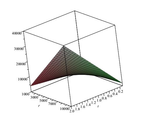
Figure 1: The graph of the lower bound of $\mathbb{H}^{g}(\frac{\partial}{\partial r})(t,r,\theta,\phi)$, when $B=e^{tr}$.

3 SENSITIVITIES IN THE DIRECTIONS $\frac{\partial}{\partial\theta}$ and $\frac{\partial}{\partial\phi}$

We begin this section by the following theorem. The sensitivity of LTB metric in the direction of $\frac{\partial}{\partial\theta}$ in the points with $\dot{R}\neq 0$ and $R^{\prime 2}\neq(\dot{R}B)^{2}$, is greater or equal than $-\ln 2+\ln|(\dot{R}B)^{2}-(R^{\prime})^{2}|-2\ln|B|.$ Since $L_{\frac{\partial}{\partial\theta}}(\frac{\partial}{\partial t})=\frac{\dot{R}}{R}\frac{\partial}{\partial\theta}$, $L_{\frac{\partial}{\partial\theta}}(\frac{\partial}{\partial r})=\frac{{R^{\prime}}}{R}\frac{\partial}{\partial\theta}$, $L_{\frac{\partial}{\partial\theta}}(\frac{\partial}{\partial\theta})=R\dot{R}\frac{\partial}{\partial t}-\frac{{RR^{\prime}}}{B^{2}}\frac{\partial}{\partial r}$, and $L_{\frac{\partial}{\partial\theta}}(\frac{\partial}{\partial\phi})=\cot\theta\frac{\partial}{\partial\phi}$, then the matrix of $L_{\frac{\partial}{\partial t}}$ in the basis $\{\frac{\partial}{\partial t},\frac{\partial}{\partial r},\frac{\partial}{\partial\theta},\frac{\partial}{\partial\phi}\}$ is

$$E=\left(\begin{array}[]{cccc}0&0&{\dot{R}}{R}&0\\ 0&0&-\frac{RR^{\prime}}{B^{2}}&0\\ \frac{\dot{R}}{R}&\frac{R^{\prime}}{R}&0&0\\ 0&0&0&\cot\theta\end{array}\right).$$

For a natural number $n$, the $(1,1)$ entry of the matrix $E^{2n}$ is $\frac{(\dot{R})^{2}((\dot{R}B)^{2}-(R^{\prime})^{2})^{n-1}}{B^{2n-2}}.$ Thus $\gamma_{2n,\frac{\partial}{\partial\theta}}\leq-\frac{2^{-2n}\dot{R}^{4}((\dot{R}B)^{2}-(R^{\prime})^{2})^{2n-2}}{B^{4n-4}}.$ In the points with $\dot{R}\neq 0$ and $R^{\prime 2}\neq(\dot{R}B)^{2}$ we have $R_{2n,\frac{\partial}{\partial\theta}}\geq\frac{\ln|-\frac{2^{-2n}\dot{R}^{4}((\dot{R}B)^{2}-(R^{\prime})^{2})^{2n-2}}{B^{4n-4}}|}{2n}=-\ln 2+\frac{4\ln|\dot{R}|}{2n}+(2n-2)\frac{\ln|(\dot{R}B)^{2}-(R^{\prime})^{2}|}{2n}-(4n-4)\frac{\ln|B|}{2n}.$ Thus $\mathbb{H}^{g}(\frac{\partial}{\partial\theta})(t,r,\theta,\phi)\geq-\ln 2+\ln|(\dot{R}B)^{2}-(R^{\prime})^{2}|-2\ln|B|.$

The lower bound of $\mathbb{H}^{g}(\frac{\partial}{\partial\theta})(t,r,\theta,\phi)$ for the case $B=e^{tr}$ and $R=t^{\frac{2}{3}}$ is sketched in figure 2.

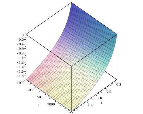
Figure 2: The graph of the lower bound of $\mathbb{H}^{g}(\frac{\partial}{\partial\theta})(t,r,\theta,\phi)$, when $B=e^{tr}$ and $R=t^{\frac{2}{3}}$.

For the direction $\frac{\partial}{\partial\phi}$ we have the next theorem. In the points $(t,r,\theta,\phi)$ which $\dot{R}\sin^{2}\theta\neq 0$ and $(\dot{R}^{2}B^{2}-R^{\prime 2})\sin^{2}\theta-B^{2}\cos^{2}\theta\neq 0,$ we have

$$\mathbb{H}^{g}(\frac{\partial}{\partial\phi})(t,r,\theta,\phi)\geq-\ln 2-2\ln|B|+\ln|(\dot{R}^{2}B^{2}-R^{\prime 2})\sin^{2}\theta-B^{2}\cos^{2}\theta|.$$

Since $L_{\frac{\partial}{\partial\phi}}(\frac{\partial}{\partial t})=\frac{\dot{R}}{R}\frac{\partial}{\partial\phi}$, $L_{\frac{\partial}{\partial\phi}}(\frac{\partial}{\partial r})=\frac{R^{\prime}}{R}\frac{\partial}{\partial\phi}$, $L_{\frac{\partial}{\partial\phi}}(\frac{\partial}{\partial\phi})=\cot\theta\frac{\partial}{\partial\phi}$, and $L_{\frac{\partial}{\partial\phi}}(\frac{\partial}{\partial\phi})=R\dot{R}\sin^{2}\theta\frac{\partial}{\partial t}-\frac{RR^{\prime}}{B^{2}}\sin^{2}\theta\frac{\partial}{\partial r}-\sin\theta\cos\theta\frac{\partial}{\partial\theta}$. Then the matrix of $L_{\frac{\partial}{\partial\phi}}$ in the basis $\{\frac{\partial}{\partial t},\frac{\partial}{\partial r},\frac{\partial}{\partial\theta},\frac{\partial}{\partial\phi}\}$ is

$$G=\left(\begin{array}[]{cccc}0&0&0&{\dot{R}}{R}\sin^{2}\theta\\ 0&0&0&-\frac{RR^{\prime}}{B^{2}}\sin^{2}\theta\\ 0&0&0&-\sin\theta\cos\theta\\ \frac{\dot{R}}{R}&\frac{R^{\prime}}{R}&\cot\theta&0\end{array}\right).$$

The entry $(1,1)$ of the matrix $G^{2n}$ is:

$$\frac{\dot{R}^{2}\sin^{2}\theta}{B^{2n-2}}((\dot{R}^{2}B^{2}-R^{\prime 2})\sin^{2}\theta-B^{2}\cos^{2}\theta)^{n-1}.$$

So,

$$\gamma_{2n,\frac{\partial}{\partial\phi}}\leq-2^{-2n}\frac{\dot{R}^{4}\sin^{4}\theta}{B^{4n-4}}((\dot{R}^{2}B^{2}-R^{\prime 2})\sin^{2}\theta-B^{2}\cos^{2}\theta)^{2n-2}.$$

Hence, in the points $(t,r,\theta,\phi),$ which $\dot{R}\sin^{2}\theta\neq 0$ and $(\dot{R}^{2}B^{2}-R^{\prime 2})\sin^{2}\theta-B^{2}\cos^{2}\theta\neq 0,$ we have

$$R_{2n,\frac{\partial}{\partial\phi}}\geq\frac{\ln|-2^{-2n}\frac{\dot{R}^{4}\sin^{4}\theta}{B^{4n-4}}((\dot{R}^{2}B^{2}-R^{\prime 2})\sin^{2}\theta-B^{2}\cos^{2}\theta)^{2n-2}|}{2n}=$$

$$-\ln 2+\frac{\ln|\dot{R}^{4}\sin^{4}\theta|}{2n}-\frac{(4n-4)\ln|B|}{2n}+\frac{2n-2}{2n}\ln|(\dot{R}^{2}B^{2}-R^{\prime 2})\sin^{2}\theta-B^{2}\cos^{2}\theta|.$$

Hence,

$$\mathbb{H}^{g}(\frac{\partial}{\partial\phi})(t,r,\theta,\phi)\geq-\ln 2-2\ln|B|+\ln|(\dot{R}^{2}B^{2}-R^{\prime 2})\sin^{2}\theta-B^{2}\cos^{2}\theta|.$$

4 EINSTEIN-VAZ SCHELLS IN THE QUANTUM FRAMEWORK

Vaz won the Second Prize in the 2014 Gravity Research Foundation Essay Competition by realizing a quantum approach to the spherical collapse of inhomogeneous dust in AdS of dimension $d=n+2$ [17], which is described by the previously analysed LeMaitre Tolman Bondi family of metrics. The model can be expressed in canonical form after a series of simplifying canonical transformations and after absorbing the surface terms [17]. By using Dirac quantization of the constraints leading to a Wheeler-DeWitt equation, two independent solutions in terms of shell wave functions supported everywhere in spacetime come out [17] (in this Section and in next one, Planck units will be used, i.e. $G=c=k_{B}=\hbar=\frac{1}{4\pi\epsilon_{0}}=1$)

$$\psi_{i}=\psi_{i}^{\left(1\right)}+A_{i}\psi_{i}^{\left(2\right)}.$$ (3)

Here $\psi_{i}^{\left(1\right)}$ represents dust shells condensing to the Schwarzschild surface (which becomes an apparent horizon) on both sides of it and $\psi_{i}^{\left(2\right)}$ represents dust shells move away from the Schwarzschild surface on either side of it where the exterior, outgoing wave is suppressed by the Boltzmann factor at the Hawking temperature for the shell, see [17] for details. It is important to emphasize that there is nothing within the theory that suggests a value for $A_{i}$ [17]. Indeed, one should need further input in order to determine these amplitudes [17]. If $0<\left|A_{i}\right|\leq 1,$ then the dust will ultimately pass through the horizon via a continued collapse arriving at a central singularity [17]. Consequently, an event horizon will form, with emission of Hawking radiation in the exterior [17]. In order to avoid the formation of the central singularity, $\left|A_{i}\right|$ must vanish [17]. Then, $\psi_{i}^{\left(1\right)}$ alone results to be the complete description of the quantum collapse [17]. But the meaning of $\psi_{i}^{\left(1\right)}$ is that each shell will condense on the Schwarzschild surface, by stopping the gravitational collapse [17]. Each shell converges to the Schwarzschild surface and a “dark star” forms [17].

Now, one can find the mass and energy spectra of this “gravitational atom” via a Schrodinger-like approach following [19]. One starts to observe that, if both the shells described by $\psi_{i}^{\left(1\right)}$ converge on the Schwarzschild surface by forming a “dark star”, then, by assuming absence of rotations and of dissipation during the collapse, such a final object will be a spherical symmetric shell. This is consistent with Einstein’s idea in 1939 of the localization of the collapsing particles within a thin spherical shell [18]. In that case, a “dark star” having mass $M$ will be subjected to the classical potential

$$V=-\frac{M^{2}}{2R},$$ (4)

which is indeed the self-interaction gravitational potential of a spherical massive shell, where $R$ is its radius [19, 21]. In the current case, $R$ is nothing else than the gravitational radius, which, in a quantum framework, is subjected to quantum fluctuations [22], due also to the potential absorption of external particles [23]. On the other hand, Eq. (4) represents also the potential of a two-particle system composed of two identical masses $M$ gravitationally interacting with a relative position $2R$. Hence, the spherical shell becomes physically equivalent to a two-particle system of two identical masses: but, clearly, as the shell’s mass $M$ does not double, one has to consider the two identical masses $M$ as being fictitious and representing the real physical shell. Let us recall the general problem of a two-particle system where the particles have different masses [19, 20]. This is a 6-dimensional problem which can be splitted into two 3-dimensional problems, that of a static or free particle, and that of a particle in a static potential if the sole interaction which is felt by the particles is their mutual interaction depending only on their relative position [19, 20]. One denotes by $m_{1}$, $m_{2}$ the masses of the particles, by $d_{1}$, $d_{2}$ their positions and by $\overrightarrow{p}_{1}$, $\overrightarrow{p}_{2}$ the respective momenta. Being $\overrightarrow{d}_{1}-\overrightarrow{d}_{2}$ their relative position, the Hamiltonian of the system reads [19, 20]

$$H=\frac{p_{1}^{2}}{2m_{1}}+\frac{p_{2}^{2}}{2m_{2}}+V(\overrightarrow{d}_{1}-\overrightarrow{d}_{2}).$$ (5)

One sets [19, 20]

$$\begin{array}[]{ccccc}m_{T}=m_{1}+m_{2},&&\overrightarrow{D}=\frac{m_{1}\overrightarrow{d}_{1}+m_{2}\overrightarrow{d}_{2}}{m_{1}+m_{2}},&&\overrightarrow{p}_{T}=\overrightarrow{p}_{1}+\overrightarrow{p}_{2},\\ \\ m=\frac{m_{1}m_{2}}{m_{1}+m_{2}}&&\overrightarrow{d}=\overrightarrow{d}_{1}-\overrightarrow{d}_{2}&&\overrightarrow{p}=\frac{m_{1}\overrightarrow{p}_{1}+m_{2}\overrightarrow{p}_{2}}{m_{1}+m_{2}}.\end{array}$$ (6)

The change of variables of Eq. (6) is a canonical transformation because it conserves the Poisson brackets [19, 20]. According to the change of variables of Eq. (6), the motion of the two particles is interpreted as being the motion of two fictitious particles: i) center of mass, having position $\overrightarrow{D}$, total mass $m_{T}$ and total momentum $\overrightarrow{p}_{T}$ and, ii) the relative particle (which is the particle associated with the relative motion), having position $\overrightarrow{d}$, mass $m,$ called reduced mass, and momentum $\overrightarrow{p}$ [19, 20]. The Hamiltonian of Eq. (5), considered as a function of the new variables of Eq. (6), becomes [19, 20]

$$H=\frac{p_{T}^{2}}{2m_{T}}+\frac{p^{2}}{2m}+V(\overrightarrow{d}).$$ (7)

The new variables obey the same commutation relations as if they should represent two particles of positions $\overrightarrow{D}$ and $\overrightarrow{d}$ and momenta $\overrightarrow{p}_{T}$ and $\overrightarrow{p}$ respectively [19, 20]. The Hamiltonian of Eq. (7) can be considered as being the sum of two terms [19, 20]:

$$H_{T}=\frac{p_{T}^{2}}{2m_{T}},$$ (8)

and

$$H_{m}=\frac{p^{2}}{2m}+V(\overrightarrow{d}).$$ (9)

The term of Eq. (8) depends only on the variables of the center of mass, while the term of Eq. (9) depends only on the variables of the relative particle. Thus, the Schrodinger equation in the representation $\overrightarrow{D},\>\overrightarrow{d}$ is [19, 20]:

$$\left[\left(-\frac{1}{2m_{T}}\triangle_{D}\right)+\left(-\frac{1}{2m}\triangle_{d}+V(d)\right)\right]\Psi\left(D,\>d\right)=E\Psi\left(D,\>d\right),$$ (10)

being $\triangle_{\overrightarrow{D}}$ and $\triangle_{\overrightarrow{d}}$ the Laplacians relative to the coordinates $\overrightarrow{D}$ and $\overrightarrow{d}$ respectively. Now, one observes that the reduced mass of the previously introduced two-particle system composed of two identical masses $M$ is

$$m=\frac{M*M}{M+M}=\frac{M}{2}.$$ (11)

In that case, by recalling that in Schwarzschild coordinates the BH center of mass coincides with the origin of the coordinate system and with the replacements

$$d\rightarrow 2R,$$ (12)

the Schrodinger equation (10) becomes

$$\left(-\frac{1}{2m}\triangle_{2R}+V(2R)\right)\Psi\left(2R\right)=E\Psi\left(2R\right).$$ (13)

Setting

$$r\equiv\frac{R}{2},$$ (14)

the potential of Eq. (4) becomes

$$V=-\frac{m^{2}}{r},$$ (15)

and the Schrodinger equation in the representation $\overrightarrow{D}=0,\>\overrightarrow{r}$ becomes

$$\left(-\frac{1}{2m}\triangle_{r}+V(r)\right)\Psi\left(r\right)=E\Psi\left(r\right),$$ (16)

that is

$$-\frac{1}{2m}\left(\frac{\partial^{2}\Psi}{\partial r^{2}}+\frac{2}{r}\frac{\partial\Psi}{\partial r}\right)+V\Psi=E\Psi.$$ (17)

The Schrodinger equation (17) is formally identical to the traditional Schrodinger equation of the $s$ states ($l=0$) of the hydrogen atom which obeys to the Coulombian potential [19, 20]

$$V(r)=-\frac{e^{2}}{r}.$$ (18)

In the potential of Eq. (15) the squared electron charge $e^{2}$ is replaced by the squared reduced mass $m^{2}.$ Thus, Eq. (17) can be interpreted as the Schrodinger equation of a particle, the “electron”, which interacts with a central field, the “nucleus”. On the other hand, this is only a mathematical artifact because the real nature of the quantum BH is in terms of Vaz’s shell. For the bound states ($E<0$) the energy spectrum is

$$E_{n}=-\frac{m^{5}}{2n^{2}}.$$ (19)

Hence, in order to completely solve the problem, one must find the relationship between the reduced mass and the total energy of Vaz’s shell. This relationship has been found in [19] as

$$E=-\frac{m}{2}.$$ (20)

By inserting this last equation in Eq. (19), a bit of algebra permits to obtain the energy spectrum

$$E_{n}=-\frac{1}{2}\sqrt{n},$$ (21)

and the corresponding mass spectrum

$$M_{n}=2\sqrt{n}.$$ (22)

5 TIME EVOLUTION OF EINSTEIN-VAZ SCHELLS

The horizon’s absence implies that Einstein-Vaz schells cannot emit radiation via the Hawking mechanism of pair production from quantum fluctuations. Hence, Einstein-Vaz schells should emit radiation like the other bodies. Following [24], from the quantum mechanical point of view, one physically interprets this radiation as energies of quantum jumps among the unperturbed levels of Eq. $(\ref{eq: BH energy levels finale.}$). In quantum mechanics, time evolution of perturbations can be described by an operator [24]

$$U(t)=\begin{array}[]{c}W(t)\;\;\;for\;0\leq t\leq\tau\\ 0\;\;\;for\;t<0\;and\;t>\tau.\end{array}$$ (23)

Then, the complete (time dependent) Hamiltonian is described by the operator

$$H(r,t)\equiv H_{0}(r)+U(t),$$ (24)

where $H_{0}(r)$ is the (time independent) Hamiltonian of the Schrodinger equation (17). Thus, considering a wave function $\psi(r,t),$ one can write the correspondent time dependent Schroedinger equation for the system

$$i\frac{d|\psi(r,t)>}{dt}=\left[H_{0}(r)+U(t)\right]|\psi(r,t)>=H(r,t)|\psi(r,t)>.$$ (25)

The state which satisfies Eq. (25) is

$$|\psi(r,t)>=\sum_{n}a_{n}(t)\exp\left(-iE_{n}t\right)|\varphi_{n}(r)>,$$ (26)

where the $\varphi_{n}(r)$ are the eigenfunctions of the time independent Schroedinger equation (17) and the $E_{n}$ are the correspondent eigenvalues. In the basis $|\varphi_{n}(r)>$, the matrix elements of $W(t)$ can be written as [24]

$$W_{ij}(t)\equiv A_{ij}\delta(t),$$ (27)

where $W_{ij}(t)=<\varphi_{i}(r)|W(t)|\varphi_{j}(r)>$ and the $A_{ij}$ are real. In order to solve the complete quantum mechanical problem described by the operator (24), one needs to know the probability amplitudes $a_{n}(t)$ due to the application of the perturbation described by the time dependent operator (23), which represents the perturbation associated with the emission of a particle. For $t<0,$ i.e. before the perturbation operator (23) starts to work, the system is in a stationary state $|\varphi_{n_{1}}(t,r)>,$ at the quantum level $n_{1},$ with energy $E_{n_{1}}=-\frac{1}{2}\sqrt{n_{1}},$ given by Eq. (21). Thus, in Eq. (26) only the term

$$|\psi_{n_{1}}(r,t)>=\exp\left(-iE_{n_{1}}t\right)|\varphi_{n_{1}}(r)>,$$ (28)

is not null for $t<0.$ This implies $a_{n}(t)=\delta_{nn_{1}}\>\>$ for $\>t<0.$ When the perturbation operator (23) stops to work, i.e. after the emission, for $t>\tau$ the probability amplitudes $a_{n}(t)$ return to be time independent, having the value $a_{n_{1}\rightarrow n}(\tau)$. In other words, for $t>\tau\>$ the system is described by the wave function $\psi_{final}(r,t),$ which corresponds to the state

$$|\psi_{final}(r,t)>=\sum_{n=1}^{n_{1}}a_{n_{1}\rightarrow n}(\tau)\exp\left(-iE_{n}t\right)|\varphi_{n}(x)>.$$ (29)

Therefore, the probability to find the system in an eigenstate having energy $E_{n}=-\sqrt{n}$, with $n<n_{1}$ for emissions, is given by

$$\Gamma_{n_{1}\rightarrow n}(\tau)=|a_{n_{1}\rightarrow n}(\tau)|^{2}.$$ (30)

By using a standard analysis [24], one obtains the following differential equation from Eq. ($\ref{eq: Schroedinger wave-function fin.})$

$$i\frac{d}{dt}a_{n_{1}\rightarrow n}(t)=\sum_{l=1}^{n}W_{n_{1}l}a_{n_{1}\rightarrow l}(t)\exp\left[i\left(\Delta E_{l\rightarrow n}\right)t\right].$$ (31)

To first order in $U(t)$, by using the Dyson series [25], one gets the solution

$$a_{n_{1}\rightarrow n}=-i\int_{0}^{t}\left\{W_{nn_{1}}(t^{\prime})\exp\left[i\left(\Delta E_{n_{1}\rightarrow n}\right)t^{\prime}\right]\right\}dt^{\prime}.$$ (32)

By inserting Eq. (27) in Eq. (32) one obtains

$$a_{n_{1}\rightarrow n}=iA_{nn_{1}}\int_{0}^{t}\left\{\delta(t^{\prime})\exp\left[i\left(\Delta E_{n_{1}\rightarrow n}\right)t^{\prime}\right]\right\}dt^{\prime}=\frac{i}{2}A_{nn_{1}}.$$ (33)

In order to find the quantities $\Gamma_{n_{1}\rightarrow n}(\tau)$ one can use a recent remarkable result of Mathur and Mehta [26], who won the third prize in the 2023 Gravity Research Foundation Essay Competition for having shown the universality of BH thermodynamics. In fact, they have shown that any Extremely Compact Object (ECO) like the Einstein-Vaz shells must have the same thermodynamic properties of standard BHs. As quantum fields just outside the surface of an ECO have a large negative Casimir energy similar to the BH Boulware vacuum, then if the thermal radiation emanating from the ECO does not fill the near-surface region at the local Unruh temperature, the consequence is that no solution of gravity equations is possible [26]. In particular, any body, included the Einstein-Vaz shells, whose radius is sufficiently close to the BH radius, will have the same thermodynamic properties as the semiclassical BH originally considered by Hawking. This implies that the temperature of an Einstein-Vaz shell having mass $M$ must be exactly the Hawking temperature of the corresponding semiclassical BH, that is $T_{H}\equiv\frac{1}{8\pi M}$ [27]. Therefore, the probability of emission of a single photon is [27]

$$\Gamma=\exp(-\frac{\omega}{T_{H}})=\exp\left(-8\pi M\omega\right).$$ (34)

For a transition between two quantum levels $n_{1}$ and $n,$ with $n<n_{1},$ one consequently finds

$$\Gamma_{n_{1}\rightarrow n}=\exp\left(-8\pi M\omega_{n_{1}n}\right),$$ (35)

where

$$\omega_{n_{1}n}\equiv M_{n_{1}}-M_{n_{1}}=2\left(\sqrt{n_{1}}-\sqrt{n}\right),$$ (36)

and Eq. (22) has been used in the last passage of Eq. (36). On the other hand, an ambiguity is present in Eq. (35). Indeed, because of the quantum transition the mass of the Einstein-Vaz shell varies from an initial value $M_{n_{1}}$ to a final value $M_{n}<M_{n_{1}}.$ Thus, it is not clear which mass must be inserted in Eq. (35) between $M_{n_{1}}$ and $M_{n}.$ The solution of this problem has been found in [23], where it has been rigorously shown, via Hawking periodicity argument [28], that the correct value to be inserted in Eq. (35) is the average value between $M_{n_{1}}$ and $M_{n},$

$$\frac{M_{n_{1}}+M_{n}}{2}$$

which indeed represents the dynamical value of the Einstein-Vaz shell mass during the quantum transition. Hence, Eq. (35) becomes

$$\Gamma_{n_{1}\rightarrow n}=\exp\left[-4\pi\left(M_{n_{1}}^{2}-M_{n}^{2}\right)\right]=\exp\left[-16\pi\left(n_{1}-n\right)\right].$$ (37)

Thus, the probability of emission between two arbitrary quantum levels of an Einstein-Vaz shell characterized by the two principal quantum numbers $n_{1}$ and $n$ scales like $\exp\left[-16\pi\left(n_{1}-n\right)\right].$ In particular, for $n=n_{1}-1$ the probability of emission has its maximum value $\sim\exp(-16\pi)$. This means that the probability is maximum for two adjacent levels, as one intuitively expects. Combining Eq. (33) with Eqs. (37) and (30) one gets

$$\begin{array}[]{c}\exp\left[16\pi\left(n-n_{1}\right)\right]=\frac{1}{4}A_{nn_{1}}^{2}\\ \\ A_{nn_{1}}=2\exp\left[8\pi\left(n-n_{1}\right)\right]\\ \\ a_{n_{1}\rightarrow n}=-i\exp\left[8\pi\left(n-n_{1}\right)\right].\end{array}$$ (38)

Then, one gets $A_{nn_{1}}\sim 10^{-11}$ for $n=n_{1}-1$, i.e. when the probability of emission has its maximum value. This implies that second order terms in $U(t)$ are $\sim 10^{-22}$ and can be neglected. Clearly, for $n<n_{1}-1$, the approximation is better because the $A_{n_{1}n}$ are even smaller than $10^{-11}$. Thus, one can write down the final form of the ket representing the state as

$$|\psi_{final}(r,t)>=\sum_{n=1}^{n_{1}}-i\exp\left[8\pi\left(n-n_{1}\right)-iE_{n}t\right]|\varphi_{n}(r)>.$$ (39)

The state (39) represents a pure final state and the states are written in terms of an unitary evolution matrix. Consequently, the time evolution of the Einstein-Vaz shells is unitary as it is requested by a quantum theory of gravity.

6 CONCLUSION REMARKS

In the classical framework we find the lower bounds for the upper bounds of the deviations of LTB metric from the Riemannian case in the directions $\frac{\partial}{\partial t}$, $\frac{\partial}{\partial\theta}$, $\frac{\partial}{\partial r}$, and $\frac{\partial}{\partial\phi}$. The reader must pay attention to this point that the directions only determine the linear dynamical systems $L_{\frac{\partial}{\partial t}}$, $L_{\frac{\partial}{\partial\theta}}$, $L_{\frac{\partial}{\partial r}}$, and $L_{\frac{\partial}{\partial\phi}}$. In fact these linear dynamical systems are coordinate free, and the sensitivities and the lower sensitivities are also coordinate free. Because they depend only to the Levi-Civita connection determines by LTB metric, which is coordinate free. In the quantum framework we analysed the properties of the Einstein-Vaz shells which are the final result of the quantum gravitational collapse arising from the Lemaitre Tolman Bondi discussed by Vaz in 2014 [17]. In fact, Vaz showed that continued collapse to a singularity can only be obtained if one combines two independent and entire solutions of the Wheeler-DeWitt equation. Forbidding such a combination leads naturally to matter condensing on the Schwarzschild surface during quantum collapse. In that way, an entirely new framework for BHs has emerged. The approach of Vaz was also consistent with Einstein’s idea in 1939 of the localization of the collapsing particles within a thin spherical shell [18]. Following [19], we derived the BH mass and energy spectra via a Schrodinger-like approach, by further supporting Vaz’s conclusions that instead of a spacetime singularity covered by an event horizon, the final result of the gravitational collapse is an essentially quantum object, an extremely compact “dark star”. This “gravitational atom” is held up not by any degeneracy pressure but by quantum gravity in the same way that ordinary atoms are sustained by quantum mechanics. Finally, we discussed the time evolution of the Einstein-Vaz shells.

Competing interests

This research has been financially supported by Shahid Bahonar University of Kerman. The Authors declare that there are no potential sources of conflict of interest in the manuscript.

References

- [1] Bianchi L., Memori di Mathematical Fiscadella Societe Italeane dilee Scienze 11, 267 (1899).
- [2] Bojowald M., Harada T., Tibrewala R., Phys. Rev. D 78, 064057 (2008).
- [3] Bondi H., Mon. Not. R. Astron. Soc. 107, 410 (1947).
- [4] Eardley D.M., Smarr L., Phys. Rev. D 19, 2239 (1979).
- [5] Herrera L., Di Prisco A., Ospino J., Entropy, 23, 1219 (2021).
- [6] Kantowski R., Sachs R.K., J. Math. Phys. 7, 443 (1966).
- [7] Lemaitre G., Ann. Soc. Sci. Bruxelles A 53, 51 (1933).
- [8] Mimoso J., Le Delliou M., Mena F., Phys. Rev. D 81, 123514 (2010).
- [9] Molaei M.R., Khajoei N., Eur. Phys. J. Plus, 131, 257 (2016).
- [10] Molaei M.R., EPL (Europhysics Letters), Volume 135, Number 4 (2021).
- [11] Shamir M.F., Astrophys. Space Sci. 330, 183 (2010).
- [12] Sussman R.A., Jaime L.G., Class. Quantum Grav. 34 245004(2017).
- [13] Tolman R.C., Proc. Natl. Acad Sci 20, 169 (1934).
- [14] Vaz C., Witten L., Singh T.P., Phys. Rev. D 63, 104020 (2001).
- [15] Wald R.M., General Relativity, University of Chicago Press, Chicago, (1984).
- [16] Zibin J.P., Scalar perturbations on Lemaitre-Tolman-Bondi spacetimes, Phys. Rev. D 78, 043504 (2008).
- [17] C. Vaz, Int. J. Mod. Phys. D 23, 1441002 (2014).
- [18] A. Einstein, Ann. Math. (Second Series) 40, 922 (1939).
- [19] C. Corda, Fortsch. Phys. 2023, 2300028 (2023).
- [20] A. Messiah, Quantum Mechanics, Vol. 1, North-Holland, Amsterdam (1961).
- [21] R. Arnowitt, S. Deser, and C. W. Misner, Phys. Rev. 120, 313 (1960).
- [22] J. D. Bekenstein, in Prodeedings of th Eight Marcel Grossmann Meeting, T. Piran and R. Ruffini, eds., pp. 92-111 (World Scientific Singapore 1999).
- [23] C. Corda, Class. Quantum Grav. 32, 195007 (2015).
- [24] A. Messiah, Quantum Mechanics, Vol. 2, North-Holland, Amsterdam (1962).
- [25] J. J. Sakurai, Modern Quantum Mechanics, Pearson Education.
- [26] S. D. Mathur and M. Mehta, Int. J. Mod. Phys. D 32, 2341003 (2023).
- [27] S. W. Hawking, Commun. Math. Phys. 43, 199 (1975).
- [28] S. W. Hawking, The Path Integral Approach to Quantum Gravity, in General Relativity: An Einstein Centenary Survey, eds. S. W. Hawking and W. Israel, (Cambridge University Press, 1979).