Generative invariance: causal extrapolation without exogeneity

Abstract

We present a new estimator for predicting outcomes in different distributional settings under hidden confounding without relying on instruments or exogenous variables. The population definition of our estimator identifies causal parameters, whose empirical version is plugged into a generative model capable of replicating the conditional law within a test environment. We check that the probabilistic affinity between our proposal and test distributions is invariant across interventions. This work enhances the current statistical comprehension of causality by demonstrating that predictions in a test environment can be made without the need for exogenous variables and without specific assumptions regarding the strength of perturbations or the overlap of distributions.

,

1 Introduction

In exploring the underlying mechanisms of real random variables $X$ and $Y$ following a joint distribution $P$, we consider the following structural causal model (SCM):

$$X\leftarrow ZV+H\alpha_{*}+\varepsilon^{\prime}_{X}\textrm{ and }Y\leftarrow X\beta_{*}+H\gamma_{*}+\varepsilon^{\prime}_{Y}$$

where $Z$, $\varepsilon^{\prime}_{X}$, $\varepsilon^{\prime}_{Y}$, $H$, and $V$ are mutually independent random variables. In this model, all variables except $Z$, which takes binary values 0 and 1 representing training and testing phases, are Gaussian-distributed. The error term $\varepsilon^{\prime}_{Y}$ has a mean of zero. The graphical structure of the model is depicted next.

We face the problem of providing predictions for covariate values $X_{1},\ldots,X_{n}$ drawn after setting $Z=1$, based on observations $(X_{1},Y_{1}),\ldots(X_{n},Y_{n})$ we obtained upon having fixed $Z=0$.

The previous set of assumptions is sufficient for making the classical instrumental variable (IV) assumptions hold [16, 1], with $Z$ acting as an instrument. The IV method, a cornerstone in countering hidden confounding within observational studies, hinges on the instrument $Z$ being orthogonal to the residuals of the response $Y$ after adjusting for the covariate $X$ through the causal parameter $\beta_{*}$. This orthogonality criterion underpins the IV method’s fundamental premise. Under the three IV assumptions, our objective encompasses minimizing the risk below with respect to $\beta\in\mathbb{R}$.

$$\mathbb{E}\left[\mathbb{E}^{2}\left[Y-X\beta\mid Z\right]\right]$$

Conditional expectation can be understood as a projection in an $L^{2}$ space of random variables, where it represents the best approximation of a random variable given the conditioning one in terms of expected squared distance. This minimization process constitutes the extent to which the conditioning variable explains the variance of the other, capturing the part that can be predicted or explained by $Z$. The minimization problem above looks for the $\beta$ that hinders $Z$ the most when trying to explain the variability of the residuals. The technical nuance that the square is taken outside the inner expectation elucidates the rationale behind the feasibility of consistently estimating the causal parameter. This subtlety is pivotal from a formal viewpoint.

Given the increasing interest in utilizing exogenous variables for domain generalization [9, 2, 10, 3, 5, 11, 14, 12, 7, 6], there is a notable drive towards marrying robustness with causal inference principles. This ambition is reflected in the efforts to generalize findings from observational settings to uncharted interventional distributions.

Drawing inspiration from the rich landscape of extrapolation in statistical analysis- see e.g. [13, 14]- we propose a novel estimator that identifies the parameters indexing a generator class that can replicate the conditional law of test environments with an arbitrarily shifted covariate distribution.

The important novelty of our approach is that its performance does not depend on the strength of perturbations and, importantly, it does not need to use exogenous variables. This marks a significant departure from conventional causal inference strategies, which have historically hinged on the collection of data across varied observational contexts to exploit the constancy of conditional distributions of response variables within a precise causal framework [8]. Our approach, therefore, presents a paradigm shift in statistical thinking regarding causal inference, moving away from traditional reliance on data diversity to ensure estimation viability.

Let $(X^{z},Y^{z})$ denote the random variable following the conditional distribution of $(X,Y)$ given intervention $Z=z\in\{0,1\}$. Denote these distributions by $P^{0}$ and $P^{1}$ respectively. This allows to detach our initial SCM into a pair of SCMs representing the observational and test distributions respectively

$$P^{0}: X^{0} \leftarrow\varepsilon_{X}, P^{1}: X^{1} \leftarrow\varepsilon_{X}+ZV,$$

$$Y^{0} \leftarrow X^{0}\beta_{*}+\varepsilon_{Y}, Y^{1} \leftarrow X^{1}\beta_{*}+\varepsilon_{Y}.$$

where $\varepsilon_{X}:=H\alpha_{*}+\varepsilon^{\prime}_{X}$ and $\varepsilon_{Y}:=H\gamma_{*}+\varepsilon^{\prime}_{Y}$. It is important to note that the newly defined residuals are not uncorrelated anymore: $\operatorname{Cov}(\varepsilon_{X},\varepsilon_{Y})=\operatorname{Cov}(H\alpha_{*}+\varepsilon^{\prime}_{X},H\gamma_{*}+\varepsilon^{\prime}_{Y})=\gamma_{*}\alpha_{*}\operatorname{Var}H=:K^{*}$, accounting for hidden confounding. Notice that the assumptions at the beginning imply that there are no interventions on the response or on the residuals.

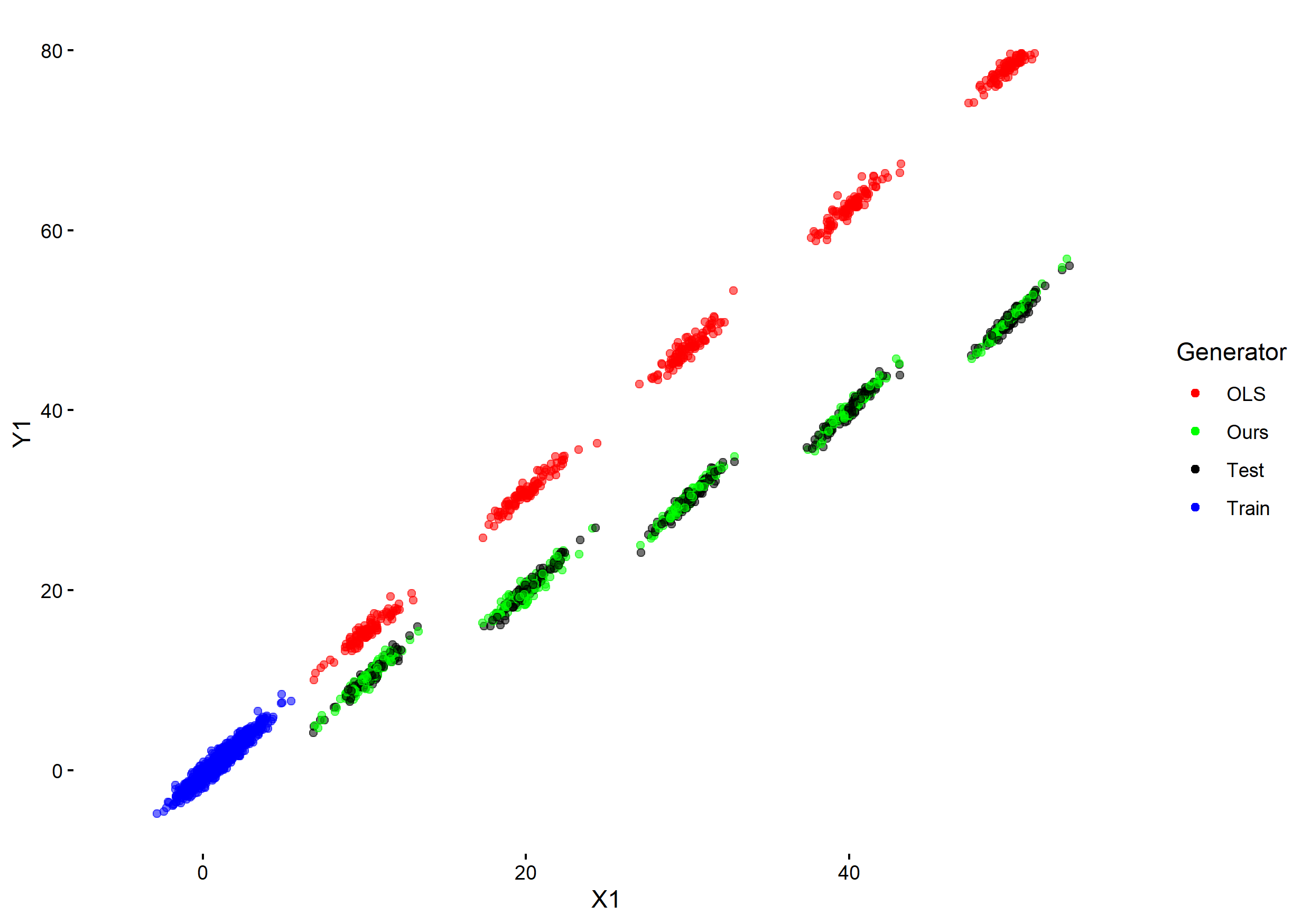
Figure 1: A sample from $P^{0}$, the training environment, is depicted in blue. Next, we sample from 5 different test environments $P^{1}$ which are colored in black. We fit an ordinary linear model to the blue data and launch red predictions. Notice how the more different the test covariates are with respect to the training set, the worse OLS performs. Our estimator can reproduce the probabilistic structure of the test environments by looking at the blue data and just at the covariate values in each test sample.

The fundamental problem here is that we just observe $(X^{1}_{1},\texttt{NA}),\ldots,(X^{1}_{n},\texttt{NA})$ from $P^{1}$. According to IV theory, using the test data as a second environment would suffice to identify the causal parameter. However, we do not have access to the values of $Y^{1}$ in a sample generated by $P^{1}$.

We will see that a positive sample variance of the test covariate distribution fundamentally enables the generation of samples that convincingly appear to originate from $P^{1}$, bridging the gap between theoretical assumptions and practical applications. This perspective acknowledges the common scenario in applied fields, where predictions are unusually made for a solitary individual in a novel domain, thereby enhancing our methodology’s applicability and relevance.

The utilization of the causal parameter for predictive purposes, while invaluable in understanding underlying mechanisms, may not always be the most effective strategy, especially under conditions of minimal perturbation. We exemplify this with the scenario where train and test distributions are the same. Although the ordinary least squares (OLS) estimator using $P^{0}$ is biased because of being the assumption $\varepsilon_{Y}\perp X^{0}$ violated, by definition we have that:

$$\mathbb{E}\left[\left(Y^{0}-X^{0}\beta_{*}\right)^{2}\right]\geq\mathbb{E}\left[\left(Y^{0}-X^{0}\beta_{\operatorname{OLS}}\right)^{2}\right]$$

where

$$\beta_{\operatorname{OLS}}:=\arg\!\min_{\beta}\mathbb{E}\left[(Y^{0}-X^{0}\beta)^{2}\right]=\frac{\operatorname{Cov}(X^{0},Y^{0})}{\operatorname{Var}X^{0}}\stackrel{{\scriptstyle K_{*}=0}}{{=}}\beta_{*}$$

Therefore, there exist situations where using the causal parameter leads to suboptimal predictive performance. Nevertheless, OLS produces an arbitrarily high mean square error when the test distribution involves a strong departure from the training one [11].

2 Population generative invariance

Assume $\operatorname{Var}X^{1}>0$. Let $\mathcal{K}$ be the real interval centered around zero with length $\sqrt{\operatorname{Var}X^{1}\operatorname{Var}\varepsilon_{Y}}$. Also define for each $K\in\mathcal{K}$

$$g_{K}:(x,\xi)\in\mathbb{R}^{2}\longmapsto(x-\mathbb{E}X^{1})\frac{K}{\operatorname{Var}X^{1}}+\xi\sqrt{\operatorname{Var}\varepsilon_{Y}-\frac{K^{2}}{\operatorname{Var}X^{1}}}$$

We show that evaluations of these functions on $X^{1}$ and noise $\xi\sim\mathcal{N}(0,1)$ are intimately connected to the joint probabilistic structure of the covariate and the response residuals at test phase.

Lemma 2.1.

For $K\in\mathcal{K}$, $g_{K}(X^{1},\xi)$ is a Gaussian random variable such that

1. $\mathbb{E}g_{K}(X^{1},\xi)=0$

2. $\operatorname{Var}g_{K}(X^{1},\xi)=\operatorname{Var}\varepsilon_{Y}$

3. $\mathbb{E}(X^{1}-\mathbb{E}X^{1})g(X^{1},\xi)=K$

As a consequence, by setting $K=K_{*}$ we can recover a copy of $(X^{1},Y^{1})$

Corollary 2.1.

$(X^{1},g_{K_{*}}(X^{1},\xi)+X^{1}\beta_{*})\sim P^{1}$

Let us set up the model

$$\mathcal{M}=\{m_{\theta}:(x,\xi)\in\mathbb{R}^{2}\longmapsto g_{K}(x,\xi)+x\beta\colon\theta=(\beta,K)\in\Theta:=\mathbb{R}\times\mathcal{K}\}$$

Functions in $\mathcal{M}$ ought to be regarded as generative models. Each element in the function class is a function $m_{\theta}$ that takes covariates $x$ and noise $\xi$, is indexed by a tuple $\theta=(\beta,K)\in\Theta$ and induces a conditional distribution: for $\theta\in\Theta$, draw $\xi\sim\mathcal{N}(0,1)$ and consider the conditional distribution of $m_{\theta}(X^{1},\xi)$ given $X^{1}=x$. In this sense, our extrapolation procedure involves a generative model consisting of two phases: first sample from the distribution of $X^{1}$ and then sample $Y^{1}$ from the conditional distribution given $X_{1}$ induced by the generator.

Remark 2.1.

The do-interventional distribution of $Y^{1}$ under do$(X^{1}=x)$ is the same as that of $m_{(\beta_{*},0)}(x,\xi)$, $\xi\sim\mathcal{N}(0,1)$.

In addressing the estimation of model parameters, we posit the determination of these true values as a theoretical risk minimization problem. This problem, intriguingly, possesses a solution that is both unique and attainable with minimal assumptions.

$$\beta^{opt},K^{opt}:=\arg\!\min_{(\beta,K)\in\Theta}\mathbb{E}\left[(Y^{0}-X^{0}\beta-(X^{0}-\mathbb{E}X^{0})K)^{2}\right]$$

Expanding the square inside of the expectation and setting derivatives to zero we arrive at the following result.

Lemma 2.2.

Whenever they exist and are unique, $\beta^{opt},K^{opt}$ need to satisfy that

$${\operatorname{Var}X^{0}}K^{opt}={(\beta_{*}-\beta_{opt})\operatorname{Var}X^{0}+K_{*}}$$

and

$$(\operatorname{Var}X^{0}+\mathbb{E}^{2}X^{0})(\beta_{*}-\beta_{opt})={K_{opt}\operatorname{Var}X^{0}-K_{*}}$$

Corollary 2.2.

If $\mathbb{E}X^{0}\neq 0$ and $\operatorname{Var}X^{0}\neq 0$ then $\beta^{opt},K^{opt}$ exist and are unique. Furthermore,

$$\beta^{opt}=\beta_{*}\textrm{ and }K^{opt}\operatorname{Var}X^{0}=K_{*}$$

Remark 2.2.

If there was access to an exogenous variable or anchor $Z$ pointing to more than one environment such that we have access to samples of both covariates and responses, we would proceed by linearly regressing out $Z$ from $Y$ and $X$ and considering the residuals resulting from these two regressions. This is equivalent to adjusting for the effect of the exogenous variable, sometimes referred to as partialling out. Assuming that an observation $(X^{z},Y^{z})$ comes from environment $z\in\{1,\ldots,N\}$ with equal probability, we have that $\mathbb{E}X=\frac{1}{\operatorname{|ImZ|}}\sum_{z=1}^{\operatorname{|ImZ|}}\mathbb{E}X^{z}$. The theoretical risk to minimize would therefore be

$$\mathbb{E}\left[\left[(1-P_{Z})(Y-X\beta-(X-\mathbb{E}X)K)\right]^{2}\right]$$

3 Empirical generative invariance

We advance our analysis by replacing $P^{0}$ with its empirical measure in the integral of the theoretical risk’s expectation, leveraging a sample from the training environment $(X^{0},Y^{0}),\ldots,(X^{0}_{n},Y^{0}_{n})\sim P^{0}$. Let $\widehat{\mu}=\frac{1}{n}\sum_{i=1}^{n}X_{i}.$

Let our estimators be defined according to

$$\widehat{\beta},\widehat{K}:=\arg\!\min_{\beta,K}\frac{1}{n}\sum_{i=1}^{n}(Y_{i}-X_{i}\beta-(X_{i}-\widehat{\mu})K)^{2}=\frac{1}{n}\sum_{i=1}^{n}\lVert Y-X\beta-(X-\widehat{\mu})K\rVert^{2}$$

Lemma 3.1 (Normal equations of empirical generative invariance).

Let $X=(X^{1},\ldots,X_{n})\in\mathbb{R}^{n\times 1}$ , $Y=(Y^{1},\ldots,Y_{n})\in\mathbb{R}^{n\times 1}$ and $1\widehat{\mu}\in\mathbb{R}^{n\times 1}$. Then $\widehat{\beta},\widehat{K}$ must satisfy

$$X^{T}X\widehat{\beta}+X^{T}(X-1\widehat{\mu})\widehat{K}=X^{T}Y$$

$$X^{T}(X-1\widehat{\mu})\widehat{\beta}+(X-1\widehat{\mu})^{T}(X-1\widehat{\mu})\widehat{K}=(X-1\widehat{\mu})^{T}Y$$

Corollary 3.1.

$\widehat{\beta}$ and $\widehat{K}$ exist and are unique if $\widehat{\mu}\neq 0$ and $\frac{1}{n}X^{T}X-\widehat{\mu}^{2}\neq 0$

Remark 3.1.

If $\operatorname{Var}X^{0}=0$, this is translated in that $X^{0}=x$ for a deterministic value $x$, what constitutes a hard intervention. We cannot recover the do-interventional distribution (involving $\beta_{*}$) in this case.

Remark 3.2.

If $\operatorname{Var}X^{1}=0$, we can still estimate $\beta^{*}$ and $K^{*}$ but the best we can do in terms of prediction is to multiply $\widehat{\beta}$ by the only covariate observation we have. Sampling from the covariate distribution in the test environment is what opens access to creating artificially correlated residuals and therefore optimal predictions. This is the reason why many methodology needs some sort of “causal regularization” when making predictions over a singleton $x$ and they proceed by modifying the proposed estimated value for the slope.

4 Experiments

First, we need to clarify how point estimates of the OLS parameter and the causal parameter $\beta^{*}$ lead to generators.

• Empirical OLS induces a generative model defined by

  $$(x,\xi)\longmapsto x\widehat{\beta}_{\operatorname{OLS}}+\widehat{\sigma}^{2}\xi$$

  where $\widehat{\sigma}^{2}$ is empirical squared residual standard error

• Empirical causal parameter induces another generative model defined by

  $$(x,\xi)\longmapsto x\widehat{\beta}+\widehat{\sigma_{*}}^{2}\xi$$

  where $\widehat{\sigma_{*}}^{2}=\frac{1}{n}\sum_{i=1}^{n}\lVert Y-X\widehat{\beta}-(X-\widehat{\mu})\widehat{K}\rVert^{2}$ is the minimum empirical risk.

We consider a grid of possible second-order moments for $V$. For each value $s$ in the grid, we sample the variance of $V$ from runif(0,s). Then we get the mean by subtracting this value from $s$. Then we generate one test dataset using this distribution for the perturbations. We hide the response values and produce predictions using our proposed generator besides the two defined above. Finally, we compute three energy scores: one corresponding to comparing the original test data with the sample synthesized by each generator. We do this for 50 times for each $s$ and average the energy scores. The results of this experiment are visible in Figure 2.

4.1 Energy statistics

For the simulations, we need a measure of similarity between $(X^{1}_{1},Y^{1}_{1})\ldots,(X^{1}_{n},Y^{1}_{n})$ and an artificial sample. Energy distance between the distribution of two random variables $Z$ and $W$ taking values in the same metric space, $\mathcal{E}(Z,W)$, is a statistical measure used to determine the similarity between two distributions [15]. Originating from the concept of Newton’s gravitational potential energy, energy statistics leverage distances between data points in metric spaces. The energy of a dataset is akin to gravitational potential energy, relying on distances to infer statistical properties.

As a consequence of Proposition 3 in [15], for $Z,W\in\mathbb{R}^{2}$ and $\delta$ the Euclidean distance therein, we have that

$$\mathbb{E}(Z,W)=2\mathbb{E}\delta(Z,W)-\mathcal{E}\delta\left(Z,Z^{\prime}\right)-\mathbb{E}\delta\left(W,W^{\prime}\right)=0$$

holds if and only if $Z$ and $W$ are identically distributed. Tilde stands for an iid copy. For us, $Z=(X^{1},Y^{1})$ and $W=(X^{1},\widetilde{Y}^{1})$, where $\widetilde{Y}^{1}$ follows the distribution of $m_{\theta}(X^{1},\xi)$ conditional to $X^{1}$ for some $\theta\in\Theta$.

Suppose that $Z_{1},\ldots,Z_{n_{1}}$ and $W_{1},\ldots,W_{n_{2}}$ are independent random samples from the distributions of $Z$ and $W$, respectively. The two-sample energy statistic corresponding to the energy distance $\mathcal{E}(Z,W)$ is

$$\widehat{\mathcal{E}}_{n_{1},n_{2}}= \frac{2}{n_{1}n_{2}}\sum_{i=1}^{n_{1}}\sum_{m=1}^{n_{2}}\left|Z_{i}-W_{m}\right|$$

$$-\frac{1}{n_{1}^{2}}\sum_{i=1}^{n_{1}}\sum_{j=1}^{n_{1}}\left|Z_{i}-Z_{j}\right|-\frac{1}{n_{2}^{2}}\sum_{\ell=1}^{n_{2}}\sum_{m=1}^{n_{2}}\left|W_{\ell}-W_{m}\right|.$$

For us $n_{1}=n_{2}$ because both samples from $Z$ and $W$ involve the same test covariate observations.

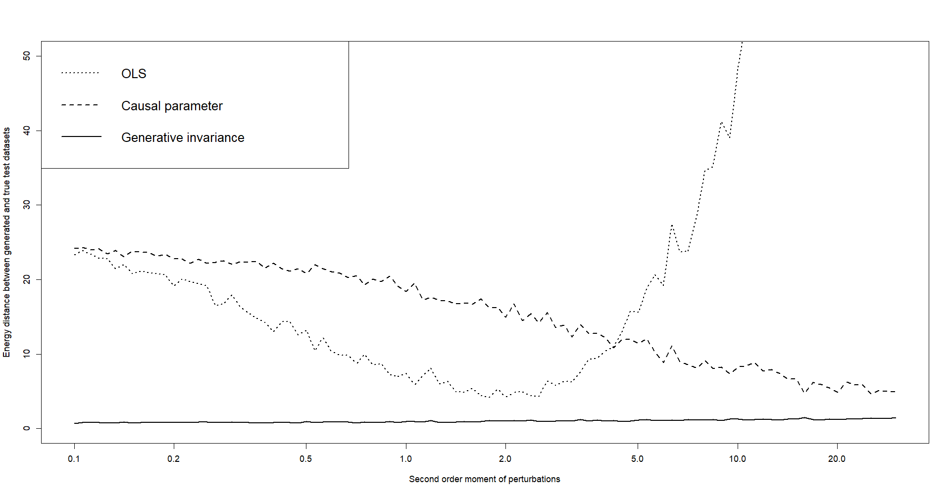
Figure 2: We fix one sampled training dataset and estimate the generator parameters using it. Then, for each different test interventional distribution of the covariate, we compute energy distance between the true sample and three artificial ones corresponding to each line type. For each fixed pertubation strength, we average across 50 test datasets. Notice how the causal parameter performs worse than OLS when the test covariate distribution is similar to that of the training set (small perturbations). Also, notice how OLS degrades arbitrarily as the strength of interventions grows - notice the log scale in the horizontal axis. Finally, our proposal seems to perform uniformly well in terms of imitating predictions uniformly well across interventions. This served as inspiration for the new concept of generative invariance with respect to energy statistics.

5 Conclusions

Our work identifies causal parameters without relying on instruments, and constructs a generative model capable of making predictions with covariate observations from a test domain, without assumptions on perturbation strength. Unlike distributional robustness literature, which requires assumptions about perturbation magnitude, our estimator is free from tunable hyperparameters. Although it assumes real Gaussian variables and no interventions on the confounders and the response during testing, these constraints simplify the mathematical framework without detracting from the significance of our contributions. We are not making any assumption on how much the training and test distributions overlap, as often needed in the literature (see e.g [4]). Our analysis does not include a comparison with alternative methods as they typically require data on both the covariate and the response for at least two distinct values of $Z$, a condition not requisite for our approach.

A crucial direction for immediate future work is the derivation of asymptotic properties. This step is essential to fully understand the behavior and reliability of our estimators as sample sizes increase. Also the derivation of approximate identifiability results when there are interventions in the latent variables or the response at test by bounding $\lVert\beta^{opt}-\beta_{*}\rVert_{\infty}$ and $\lVert K^{opt}-K_{*}\rVert_{\infty}$

Future work offers promising avenues, including extending our approach to high-dimensional settings where $X$ is p-dimensional, and exploring nonlinear models. The class $\mathcal{M}$ looks like a semiparametric model when replacing $x\beta$ by a richer family of functions. The part of the model concerning $g_{K}$ is always going to be parametric, very likely of the same dimension as the number of covariates. These directions not only promise to broaden the applicability of our methodology but also to enhance its predictive power in complex data landscapes.

References

- [1] J. D. Angrist, G. W. Imbens, and D. B. Rubin. Identification of causal effects using instrumental variables. Journal of the American statistical Association, 91(434):444–455, 1996.
- [2] M. Arjovsky, L. Bottou, I. Gulrajani, and D. Lopez-Paz. Invariant risk minimization. arXiv preprint arXiv:1907.02893, 2019.
- [3] R. Christiansen, N. Pfister, M. E. Jakobsen, N. Gnecco, and J. Peters. A causal framework for distribution generalization. IEEE Transactions on Pattern Analysis and Machine Intelligence, 44(10):6614–6630, 2021.
- [4] C. García-Meixide and M. Matabuena. Causal survival embeddings: non-parametric counterfactual inference under censoring, 2023.
- [5] A. Henzi, X. Shen, M. Law, and P. Bühlmann. Invariant probabilistic prediction. arXiv preprint arXiv:2309.10083, 2023.
- [6] D. Krueger, E. Caballero, J.-H. Jacobsen, A. Zhang, J. Binas, D. Zhang, R. Le Priol, and A. Courville. Out-of-distribution generalization via risk extrapolation (rex). In International Conference on Machine Learning, pages 5815–5826. PMLR, 2021.
- [7] Y. Lin, H. Dong, H. Wang, and T. Zhang. Bayesian invariant risk minimization. In Proceedings of the IEEE/CVF Conference on Computer Vision and Pattern Recognition, pages 16021–16030, 2022.
- [8] J. Peters, P. Bühlmann, and N. Meinshausen. Causal inference by using invariant prediction: identification and confidence intervals. Journal of the Royal Statistical Society Series B: Statistical Methodology, 78(5):947–1012, 2016.
- [9] M. Rojas-Carulla, B. Schölkopf, R. Turner, and J. Peters. Invariant models for causal transfer learning. The Journal of Machine Learning Research, 19(1):1309–1342, 2018.
- [10] D. Rothenhäusler, P. Bühlmann, and N. Meinshausen. Causal dantzig: Fast inference in linear structural equation models with hidden variables under additive interventions. The Annals of Statistics, 47(3):1688–1722, 2019.
- [11] D. Rothenhäusler, N. Meinshausen, P. Bühlmann, and J. Peters. Anchor regression: Heterogeneous data meet causality. Journal of the Royal Statistical Society Series B: Statistical Methodology, 83(2):215–246, 2021.
- [12] S. Saengkyongam, L. Henckel, N. Pfister, and J. Peters. Exploiting independent instruments: Identification and distribution generalization. In International Conference on Machine Learning, pages 18935–18958. PMLR, 2022.
- [13] S. Saengkyongam, E. Rosenfeld, P. Ravikumar, N. Pfister, and J. Peters. Identifying representations for intervention extrapolation. arXiv preprint arXiv:2310.04295, 2023.
- [14] X. Shen, P. Bühlmann, and A. Taeb. Causality-oriented robustness: exploiting general additive interventions. arXiv preprint arXiv:2307.10299, 2023.
- [15] G. J. Székely and M. L. Rizzo. The energy of data. Annual Review of Statistics and Its Application, 4:447–479, 2017.
- [16] P. G. Wright. The tariff on animal and vegetable oils. Number 26. Macmillan, 1928.