Extended Fayans energy density functional: optimization and analysis

Abstract

The Fayans energy density functional (EDF) has been very successful in describing global nuclear properties (binding energies, charge radii, and especially differences of radii) within nuclear density functional theory. In a recent study, supervised machine learning methods were used to calibrate the Fayans EDF. Building on this experience, in this work we explore the effect of adding isovector pairing terms, which are responsible for different proton and neutron pairing fields, by comparing a 13D model without the isovector pairing term against the extended 14D model. At the heart of the calibration is a carefully selected heterogeneous dataset of experimental observables representing ground-state properties of spherical even-even nuclei. To quantify the impact of the calibration dataset on model parameters and the importance of the new terms, we carry out advanced sensitivity and correlation analysis on both models. The extension to 14D improves the overall quality of the model by about 30%. The enhanced degrees of freedom of the 14D model reduce correlations between model parameters and enhance sensitivity.

Keywords: model calibration, numerical optimization, statistical analysis, sensitivity analysis, density functional theory, nuclear pairing

1 Introduction

Nuclear density functional theory (DFT) [1, 2, 3] is a quantum many-body method applicable across the whole nuclear landscape. At the heart of nuclear DFT lies the energy density functional (EDF) that represents an effective internucleon interaction. The EDF is a functional of various nucleonic densities and currents, which are usually assumed to be local. The EDF coupling constants are usually adjusted to experimental data and—in many cases—to selected nuclear matter parameters. The validated global EDFs often provide a level of accuracy typical of phenomenological approaches based on parameters locally optimized to the experiment and enable extrapolations toward particle drip lines and beyond [4].

The EDF developed by S.A. Fayans and collaborators [5, 6, 7, 8] turned out to be particularly useful since it was designed to describe the ground-state properties of finite nuclei. The volume part of the functional was adjusted to reproduce the microscopic equation of state of the nucleonic matter [6]. In this sense the functional could be considered “universal.” By employing a density-dependent pairing functional with gradient terms, the Fayans EDF was able to explain the odd-even staggering effect in charge radii [5, 7].

In [9], detailed analysis of the Fayans EDF was carried out. Various optimization strategies were explored to arrive at a consistent description of odd-even staggering of binding energies and charge radii. Next, the functional was extended to weakly bound nuclei [10] and long isotopic chains, to that end invoking Hartree–Fock–Bogoliubov (HFB) pairing instead of the simpler Bardeen–-Cooper–-Schrieffer (BCS) approach. These functionals were subsequently used for the interpretation of experimental data on charge radii [11, 12, 13, 14, 15, 16, 17, 18, 19, 20, 21, 22, 23, 24].

Recently, the Fayans functional was extended by allowing separate pairing strengths for proton and neutrons, that is, pairing isovector terms. Indeed, in order to accommodate the experimental odd-even mass staggering, the effective pairing interaction in atomic nuclei requires larger strength in the proton pairing channel than in the neutron pairing channel [25]. Such an extension enhances the flexibility to accommodate the radius trends in isotopic chains also in heavier nuclei; for a preliminary application see [26].

Following the previous large-scale calibration studies of Skyrme EDFs [27, 28, 29, 30], in [31] various supervised machine learning methods were employed to optimize the Fayans EDF. Building on this experience, in this study we explore the effect of adding isovector pairing terms. This is done based on the dataset of [9]. We compare fits with and without the pairing isovector terms and provide advanced sensitivity analysis of the resulting model.

2 The Fayans functional

The Fayans EDF is a nonrelativistic energy density functional similar to the widely used Skyrme functional [1], but with more flexibility in density dependence and pairing. We use it here in the form of the original FaNDF0 parameterization [6]. The functional is formulated in terms of particle density $\rho_{t}$, kinetic density $\tau_{t}$, spin-orbit current $\bm{J}_{t}$, and pairing densities $\breve{\rho}_{t}$, where the isospin index $t$ labels isoscalar ($t=0$) and isovector ($t=1$) densities; for details see A. The isoscalar and isovector densities can be expressed in terms of proton ($p$, $\tau_{3}=-1$) and neutron ($n$, $\tau_{3}=+1$) densities, for example,

$$\rho_{0}=\rho_{n}+\rho_{p},~{}~{}\rho_{1}=\rho_{n}-\rho_{p},$$ (1)

and similarly for the other densities. It is convenient to use also the dimensionless densities

$$x_{t}=\frac{\rho_{t}}{\rho_{\mathrm{sat}}}\;,\;x_{\mathrm{pair}}=\frac{\rho_{0}}{\rho_{\mathrm{pair}}}\;,$$ (2)

where $\rho_{\mathrm{sat}}$ and ${\rho_{\mathrm{pair}}}$ are scaling parameters of the Fayans EDF.

Within DFT, the total energy of the system is given by $E=\int d^{3}r\mathcal{E}(\bm{r})$, where the local energy density $\mathcal{E}$ is a functional of the local isoscalar and isovector particle and pairing densities and currents. The energy density of the Fayans EDF is composed from volume, surface, spin-orbit, and pairing terms. We use it here in the following form:

$$\mathcal{E}_{\mathrm{Fy}} = \mathcal{E}_{\mathrm{Fy}}^{\mathrm{v}}(\rho)+\mathcal{E}_{\mathrm{Fy}}^{\mathrm{s}}(\rho)+\mathcal{E}_{\mathrm{Fy}}^{\mathrm{ls}}(\rho,\bm{J})+\mathcal{E}_{\mathrm{Fy}}^{\mathrm{pair}}(\rho,\breve{\rho})$$ (3a)

$$\mathcal{E}_{\mathrm{Fy}}^{\mathrm{v}} = {\textstyle\frac{1}{3}}\varepsilon_{F}\rho_{\mathrm{sat}}\left[{a_{+}^{\mathrm{v}}}\frac{1\!-\!{h_{1+}^{\mathrm{v}}}x_{0}^{{\sigma}}}{1\!+\!{h_{2+}^{\mathrm{v}}}x_{0}^{{\sigma}}}x_{0}^{2}+{a_{-}^{\mathrm{v}}}\frac{1\!-\!{h_{1-}^{\mathrm{v}}}x_{0}}{1\!+\!{h_{2-}^{\mathrm{v}}}x_{0}}x_{1}^{2}\right]$$ (3b)

$$\mathcal{E}_{\mathrm{Fy}}^{\mathrm{s}} = {\textstyle\frac{1}{3}}\varepsilon_{F}\rho_{\mathrm{sat}}\frac{a_{+}^{\mathrm{s}}r_{s}^{2}(\bm{\nabla}x_{0})^{2}}{1+h_{\nabla}^{\mathrm{s}}r_{s}^{2}(\bm{\nabla}x_{0})^{2}}$$ (3c)

$$\mathcal{E}_{\mathrm{Fy}}^{\mathrm{ls}} = \frac{4\varepsilon_{F}r_{s}^{2}}{3\rho_{\mathrm{sat}}}\left(\kappa\rho_{0}\bm{\nabla}\cdot\bm{J}_{0}+\kappa^{\prime}\rho_{1}\bm{\nabla}\cdot\bm{J}_{1}+g\bm{J}_{0}^{2}+g^{\prime}\bm{J}_{1}^{2}\right)$$ (3d)

$$\mathcal{E}_{\mathrm{Fy},q}^{\mathrm{pair}} = \frac{4}{\varepsilon_{F}}{3\rho_{\mathrm{sat}}}{\breve{\rho}_{q}}^{2}\left[f_{\mathrm{ex},+}^{\xi}-\tau_{3q}f_{\mathrm{ex},-}^{\xi}+h_{1+}^{\xi}x_{\mathrm{pair}}^{\gamma}+h_{\nabla}^{\xi}r_{s}^{2}(\bm{\nabla}x_{\mathrm{pair}})^{2}\right].$$ (3e)

Several EDF parameters are fixed a priori. These are $\hbar^{2}/2m_{p}=20.749811$ MeV fm², $\hbar^{2}/2m_{n}=20.721249$ MeV fm², $e^{2}=1.43996448$ MeV fm, $\rho_{\mathrm{sat}}=0.16$ fm^-3, $\rho_{\mathrm{pair}}=\rho_{\mathrm{sat}}$, $\sigma=1/3$, and $\gamma=2/3$. The saturation density $\rho_{\mathrm{sat}}$ determines also the auxiliary parameters Wigner–Seitz radius $r_{s}=(3/4\pi\rho_{\mathrm{sat}})^{1/3}$ and Fermi energy $\varepsilon_{F}=(9\pi/8)^{2/3}\hbar^{2}/2mr_{s}^{2}$. The saturation density $\rho_{\mathrm{sat}}$ is a fixed scaling parameter, not identical to the physical equilibrium density $\rho_{\mathrm{eq}}$ that is a result of the model. Note the factor 4 in the pairing functional (3e); the paper [9] had a misprint at that place showing only a factor of 2.

Besides the Fayans nuclear energy $\mathcal{E}_{\mathrm{Fy}}$, the total energy accounts also for Coulomb energy (direct and exchange) and the center-of-mass correction term. These are standard terms without free parameters [1], and hence they are not documented here. The pairing functional is complemented by prescription for the cutoff in pairing space, which is explained in A. Altogether, the discussed Fayans model has $p=13(14)$ free parameters: six in the volume term ($a_{\pm}^{\mathrm{v}},h_{1\pm}^{\mathrm{v}},h_{2\pm}^{\mathrm{v}}$), two in the surface term ($a_{+}^{\mathrm{s}},h_{\nabla}^{\mathrm{s}}$), two in the spin-orbit term ($\kappa,\kappa^{\prime}$), and three (four) in the pairing term ($f_{\mathrm{ex},+}^{\xi},[f_{\mathrm{ex},-}^{\xi}],h_{+}^{\xi},h_{\nabla+}$). Five of the six volume parameters can be expressed in terms of five nuclear matter properties (NMPs), namely, equilibrium density $\rho_{\mathrm{eq}}$, energy per nucleon $E_{\rm B}/A$, incompressibility $K$, symmetry energy $J$, and slope of symmetry energy $L$; for their definition in terms of the energy functional see B. There remains only $h_{2-}^{\mathrm{v}}$ as a direct volume parameter. This recoupling has the advantage that the rather technical model parameters are replaced by more physical droplet model constants. We use the parameters in this recoupled form.

The numerical treatment is based on the spherical Hartree–Fock code [32]. The spherical DFT equations are solved on a numerical 1D radial grid with five-point finite differences for derivatives, a spacing of 0.3 fm, and a box size from 9.6 fm for light nuclei to 13.8 fm for heavy ones. The solution is determined iteratively by using the accelerated gradient technique. For the BCS pairing cutoff, we use a soft cutoff with the Fermi profile [33]; see A for details.

A few words are in order about the numerical realization of computing nuclear properties for the Fayans functional. The largest part of the computations, namely, preparing the observables for the optimization routine POUNDerS and subsequent analysis of the results, is done with a spherical 1D code. The radial wavefunctions and fields are represented on a spatial grid along radial directions. The ground state is found by using accelerated gradient iterations on the energy landscape. The numerical basics are explained in detail in [32]. In section 5.2 we also analyze the predictions for deformed nuclei along a selection of isotopic chains. These embrace also deformed nuclei. The deformed calculations are performed by using a cylindrical 2D grid in coordinate space. As in the 1D case, accelerated gradient iteration coupled to the BCS iterations is used to find the ground state. The 2D code, coined SkyAx, is explained in detail in [34].

3 Optimization and local analysis

3.1 Problem definition: the objective function

The FaNDF DFT package uses the parameterized Fayans EDF to obtain the model value $m(\bm{\nu}_{i};\bm{x})$ of a given observable for a given nucleus, both specified by the input $\bm{\nu}_{i}$, at a desired parameter-space point $\bm{x}\in\mathbb{R}^{p}$. For a particular dataset $\mathcal{D}=\left\{(\bm{\nu}_{i},d_{i})\right\}_{i=1}^{n}$ we construct the weighted least-squares objective function

$$f(\bm{x};\mathcal{D})=\sum_{i=1}^{n}\left(\frac{d_{i}-m(\bm{\nu}_{i};\bm{x})}{w_{i}}\right)^{2}=\sum_{i=1}^{n}\delta_{i}^{2}(\bm{x};\mathcal{D}),$$ (3d)

where the $w_{i}$, which we refer to as “adopted errors,” are positive numbers discussed below and where $\delta_{i}$ are residuals. Note that the residuals are dimensionless by virtue of the weights $w_{i}$. This allows the accumulation of contributions from different physical observables. Effectively, we deal with a dimensionless dataset $\tilde{\mathcal{D}}=\left\{(\bm{\nu}_{i},\tilde{d}_{i})\right\}_{i=1}^{n}$ with

$$\tilde{d}_{i}\equiv\frac{d_{i}}{w_{i}},$$ (3e)

which allows us to compare variations of $\tilde{d}_{i}$ from physically different types of observables [35, 36].

In this paper we use the iterative derivative-free optimization software POUNDerS [37] to approximate a nonlinear least-squares local minimizer $\hat{\bm{x}}$ associated with the dataset such that

$$f(\hat{\bm{x}};\tilde{\mathcal{D}})\approx\min_{\bm{x}\in\mathbb{R}^{p}}\,f(\bm{x};\tilde{\mathcal{D}}).$$ (3f)

3.2 Regression analysis

Optimization has reached its goal if an approximate minimum of the objective function $f$ is found. In addition to the minimum point defining the optimal parameter set $\hat{\bm{x}}$, the behavior of $f$ around $\hat{\bm{x}}$ carries useful information; the local behavior determines the response to slightly varying conditions such as noise in the data. When endowed with a particular statistical interpretation, the local behavior determines a range of reasonable parameters by using $f$ as the generator of a probability distribution in parameter space. The profile of $f$, soft or steep, determines the width of the probability distribution near $\hat{\bm{x}}$. The vicinity near $\hat{\bm{x}}$ can be described by a Taylor expansion with respect to $\bm{x}$. The first derivative at a minimum disappears; that is, $\partial_{x_{\alpha}}f=0$. The second derivative at a minimum can be approximated as

$$\partial_{x_{\alpha}}\partial_{x_{\beta}}f\big{|}_{\hat{\bm{x}}}\approx C_{\alpha\beta}=\sum_{i}J_{i\alpha}J_{i\beta},$$ (3g)

where $\hat{J}\equiv J_{i\alpha}=\partial_{x_{\alpha}}\delta_{i}$ is the Jacobian matrix and $\hat{C}\equiv C_{\alpha\beta}$ is merely shorthand for an approximation of the second derivative of the objective function, which characterizes the leeway of the model parameters. In certain statistical settings, the inverse $\hat{C}^{-1}$ can be interpreted as proportional to an approximate covariance matrix. Its diagonal elements give an estimate of the standard deviation $\hat{\sigma}_{\alpha}$ of parameter $x_{\alpha}$ as

$$\hat{\sigma}_{\alpha}=\hat{\sigma}\sqrt{(\hat{C}^{-1})_{\alpha\alpha}}\;,\;\hat{\sigma}^{2}=\frac{f(\hat{\bm{x}})}{n-p}\;.$$ (3h)

The value $\hat{\sigma}_{\alpha}$ sets a natural scale for variations of $x_{\alpha}$: variations less (larger) than $\hat{\sigma}_{\alpha}$ are considered small (large). This suggests the introduction of dimensionless parameters

$$\tilde{x}_{\alpha}=\frac{x_{\alpha}}{\hat{\sigma}_{\alpha}},$$ (3i)

which will play a role in the sensitivity analysis of section 4.3.

The matrix $(\hat{C}^{-1})_{\alpha\beta}$ can be used to approximate not only the variances of each parameter but also the correlations between different parameters. This matrix depends on the physical dimensions of the parameters. Rescaling it using the dimensionless parameters yields the matrix

$$R_{\alpha\beta}=\frac{(\hat{C}^{-1})_{\alpha\beta}}{\sqrt{(\hat{C}^{-1})_{\alpha\alpha}(\hat{C}^{-1})_{\beta\beta}}}.$$ (3j)

The square of the covariances, $R_{\alpha\beta}^{2}$, defines the coefficients of determination (CoDs), which will be discussed in section 4.2.

3.3 Calibration strategy and selection of data

At this point, it is worth recapitulating the history of our Fayans EDF parameterizations based on careful calibrations of large, heterogeneous datasets. The first fit, which was published in [9] and is called $Fy(\Delta r)$, calibrated the functional without the isovector pairing parameter $f_{\mathrm{ex},-}^{\xi}$ and treated pairing at the BCS level. While the present study’s dataset is an evolution of the datasets from this first fit and from [31], they are all nearly identical. The BCS pairing inhibits application of $Fy(\Delta r)$ for weakly bound nuclei. The next stage aimed to include the measured charge radius of the neutron-deficient ³⁶Ca, which required the use of HFB pairing. The refit including ³⁶Ca delivered the parameterization $Fy(\Delta r,{\rm HFB})$ [10], which can be applied without constraints on the binding strength. Both parameter sets deliver a fairly good reproduction of nuclear bulk properties over the chart of nuclei together with differential charge radii along the Ca isotopic chain. However, subsequent applications revealed that the reproduction of differential radii in heavier nuclei was deficient. To allow more flexibility, one must allow different pairing strengths for protons and neutrons, which amounts to activating the parameter $f_{\mathrm{ex},-}^{\xi}$. For first explorations, isotopic radius differences in Sn and Pb were added to the optimization dataset, which resulted in a substantial improvement for all isotopic radius differences without loss in other observables [26]. Here, we scrutinize the impact of $f_{\mathrm{ex},-}^{\xi}$ as such (i.e., without changing the dataset).

In this study we compare the optimization, nonlinear regression analysis, and sensitivity analysis results for a baseline problem with the Fayans EDF using $p=13$ free model parameters and fixed $f_{\mathrm{ex},-}^{\xi}=0$ against the $p=14$ version of the baseline problem with $f_{\mathrm{ex},-}^{\xi}$ freed. The two problems are constructed with the same dataset, $\mathcal{D}$, which comprises $n=194$ observables that are associated with 69 different spherical, ground-state, even-even nucleus configurations. Table 1 shows a breakdown of the physical observables by class. The energy staggering (last two rows) is defined by means of the three-point energy difference between neighboring even-even isotopes for $\Delta^{(3)}E_{n}$ and isotones for $\Delta^{(3)}E_{p}$. It provides experimental data to inform the pairing functional. The dataset used for optimizing the Fayans EDF consists of binding energies and their differences and key properties of the charge form factor [38] such as charge radius, diffraction (or box-equivalent) radius, and surface thickness. The individual data are listed in tables 5 and 6.

Table 1: The classes of physical observables $d_{i}$ ($i=1,\dots 194$) included in this study.

Class	Symbol	Number of observables
Binding energy	$E_{\rm B}$	60
Diffraction radius	$R_{\rm box}$	28
Surface thickness	$\sigma$	26
Charge radius	$r_{\rm ch}$	54
Proton single-level energy	$\epsilon_{\mathrm{ls,p}}$	3
Neutron single-level energy	$\epsilon_{\mathrm{ls,n}}$	4
Differential radii	$\delta\langle r^{2}\rangle$	3
Neutron radius staggering	$\Delta^{(3)}E_{n}$	5
Proton radius staggering	$\Delta^{(3)}E_{p}$	11

The adopted errors ($w_{i}$) associated with the residuals in the dataset are basically taken from those in [9] and are provided in C. Their choice is a compromise. Typically, the adopted errors are tuned such that the average variance from (3h) fulfills $\hat{\sigma}^{2}=1$ [35, 36]. This works only approximately in our case because the model has a systematic error associated with its mean-field approximation neglecting correlations. This error has been estimated by computing collective ground-state correlations beyond DFT throughout the chart of isotopes [39]. The adopted errors are taken from previous fits for which the criterion $\hat{\sigma}^{2}=1$ was approximately fulfilled. The data were selected such that the systematic error remains below the adopted error. The more versatile Fayans functional considered here produces better fits, and one is tempted to reduce the $w_{i}$ to meet the criterion. But then one may lose a great amount of fit data, which would reduce the predictive power of the fit. We thus continue to use the inherited adopted errors and accept that we deal then typically with $\hat{\sigma}^{2}\approx 1/4$ for 13D and $\approx 1/5$ for 14D. A special case is the few data on spin-orbit splittings of single-particle levels; their uncertainty is taken as rather large because single-particle energies are indirectly deduced from neighboring odd nuclei, which adds another bunch of uncertainties.

Similar to the previous fits of the Fayans EDF [9, 40], the dataset includes three-point staggering of binding energies for calibrating pairing properties; see table 7. In this case, however, the dataset includes even-even staggering as opposed to even-odd staggering; see [9] for more details.

A few crucial differential charge radii in Ca are included in the fit data; see table 8. These were decisive for determining the advanced gradient terms in the Fayans EDF related to the parameters $h_{\nabla}^{\mathrm{s}}$ and $h_{\nabla}^{\xi}$. For a detailed discussion of the physics implications see [9]. The additional data points on differential charge radii were given small adopted errors to force good agreement for these new data points.

3.4 Parameter scaling and parameter boundaries

Table 2: The length scales $\sigma_{\mathrm{scale}}$ used to define the linear scaling of each parameter at the starting point $\bm{x}_{1}$, which was the best result in [31]; the result of the 13D optimization $\hat{\bm{x}}_{13\mathrm{D}}$; and the result of the 14D optimization $\hat{\bm{x}}_{14\mathrm{D}}$. The units for $\rho_{\mathrm{eq}}$ are in fm^-3; for $E_{\rm B}/A,K,J,$ and $L$, the units are in MeV. All other parameters are dimensionless.

	$\sigma_{\mathrm{scale}}(\bm{x}_{1})$	$\sigma_{\mathrm{scale}}(\hat{\bm{x}}_{13D})$	$\sigma_{\mathrm{scale}}(\hat{\bm{x}}_{14D})$
$\kappa$	0.0152	0.0121	0.0337
$\kappa^{\prime}$	0.546	0.606	0.452
$a_{+}^{\mathrm{s}}$	0.0392	0.0328	0.0438
$h_{\nabla}^{\mathrm{s}}$	0.162	0.125	0.250
$E_{\rm B}/A$	0.125	0.125	0.125
$\rho_{\mathrm{eq}}$	0.00484	0.00403	0.00536
$K$	16.5	15.3	21.1
$J$	3.18	3.04	2.70
$L$	33.5	29.0	19.6
$h_{2-}^{\mathrm{v}}$	27.2	78.7	10900
$f_{\mathrm{ex},+}^{\xi}$	0.0592	0.0450	0.0917
$h_{1+}^{\xi}$	0.0832	0.0635	0.128
$h_{\nabla}^{\xi}$	0.368	0.286	0.742
$f_{\mathrm{ex},-}^{\xi}$	2.17	2.18	0.853

The model parameters used in the functional have different physical units. In addition, empirical studies of the objective function at the different starting points used in the study reveal that the characteristic length scales of the objective function along different parameters can vary by several orders of magnitude at each point and that these length scales can differ significantly between points. To aid the optimization and subsequent analysis, we determined independently at each of several key parameter-space points a linear scaling of the parameter space such that objective function values change by a similar amount in magnitude due to offsets along each parameter by the same amount in the scaled space. The length scales used to scale our parameter space are given in table 2.

While in a previous FaNDF study [31] special techniques were used to maintain optimizations within a constrained region in which the software was expected to be numerically stable, for this study we performed only unconstrained optimizations in accord with (3f) and without major issues.

4 Results

4.1 Optimization with POUNDerS

The $p=13$ optimization, referred to as 13D in the following, was started from the best result, $\bm{x}_{1}$, reported in [31]. The least-squares approximation obtained, called $\hat{\bm{x}}_{13\mathrm{D}}$ (see table 3), is different from $\bm{x}_{1}$ due to improvements made to the software and the aforementioned changes to the dataset. The resulting Fayans EDF parameterization is called Fy($\Delta r$, 13D). ECNoise tools based on [41, 42, 43] were used to obtain forward-difference approximations to the gradient of the objective function and the Jacobian of the residual function, $\hat{J}(\hat{\bm{x}}_{13\mathrm{D}})\equiv\hat{J}_{13\mathrm{D}}\in\mathbb{R}^{n\times p}$, which are needed for assessing the quality of the POUNDerS solution, nonlinear regression analysis, and sensitivity analysis.

The $p=14$ optimization, referred to as 14D in the following, was started from both $\bm{x}_{1}$ and $\hat{\bm{x}}_{13\mathrm{D}}$, with both effectively yielding the same least-squares approximation $\hat{\bm{x}}_{14\mathrm{D}}$; see table 3. For the optimization started at the former point, the length scale along $h^{\mathrm{v}}_{2-}$ changed significantly enough over the optimization that the objective function was eventually evaluated at points where the software failed. This necessitated determining a new linear scaling law at an intermediate point and restarting the optimization from that point using the new scaling. The gradient and Jacobian, $\hat{J}_{14\mathrm{D}}$, were obtained with ECNoise in an identical way to that for the 13D solution. The resulting Fayans EDF parameterization is called Fy($\Delta r$, 14D).

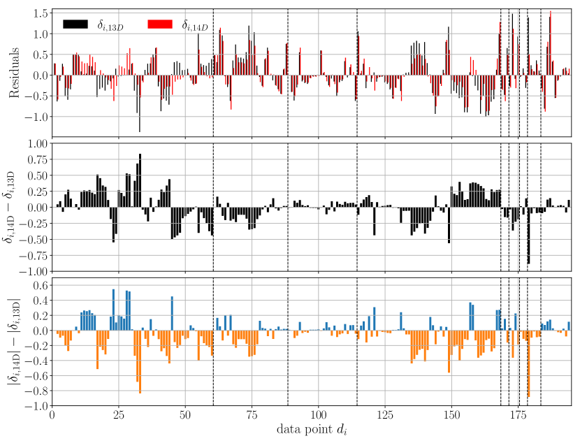
Figure 1: (top) Residual values for the 13D and 14D solutions. (middle) Change in residual values between the 13D and 14D solutions. (bottom) Change in residual magnitude between the 13D and 14D solutions. A negative value indicates that the magnitude of the associated residual decreased as a result of freeing $f_{\mathrm{ex},-}^{\xi}$. The elements are grouped in observable classes of table 1 with an ordering, from left to right, of $E_{\rm B}$, $R_{\mathrm{box}}$, $\sigma$, $r_{\mathrm{ch}}$, $\epsilon_{\mathrm{ls,p}}$, $\epsilon_{\mathrm{ls,n}}$, $\delta\langle r^{2}\rangle$, $\Delta^{(3)}E_{n}$, and $\Delta^{(3)}E_{p}$.

The top panel of figure 1 shows the residuals elementwise for both solutions. The bottom panel presents the change of the absolute value of the residuals, with negative (positive) values indicating a gain (loss) in quality of the agreement to data. The residuals are grouped by classes of observables with subgrouping into isotopic or isotonic chains where possible. Large changes between the two parameterization are seen for binding energies and charge radii, moderate changes for diffraction radii, and small differences for surface thicknesses. The bottom panel shows that the extension from 13D to 14D, while generally beneficial, can decrease agreement with experiment for some observables. To quantify this effect, we now inspect partial sums of the objective function $f$ rather than single residuals.

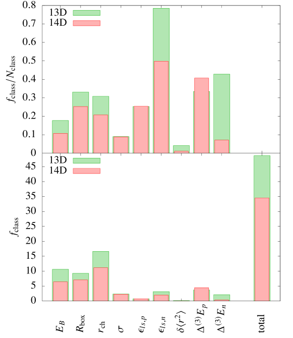
Figure 2: Breakdown of the contributions to the total objective function $f$ by observable class (see table 1) for the Fy($\Delta r$,13D) and Fy($\Delta r$,14D) parameterizations (see table 3). Presented are the (bottom) summed contribution $f_{\mathrm{class}}$ within a class and the (top) average contribution per data point $f_{\mathrm{class}}/N_{\mathrm{class}}$, where $N_{\mathrm{class}}$ is the number of data points in the given class.

The lower panel of figure 2 shows the total objective function $f$ (rightmost bar) and the partial contributions $f_{\mathrm{class}}$ summed over each class of observables (energy, radii, etc.) as indicated. The upper panel complements the information by showing the $f_{\mathrm{class}}$ per data point for each class. Adding $f_{\mathrm{ex},-}^{\xi}$ to the set of optimized parameters results in a clear gain in quality for most observables. Several observables (surface thickness, proton spin-orbit splitting, and proton gap) are hardly affected by this change. The most significant improvement is seen for the neutron gap.

The $\chi^{2}$ per datum (upper panel) shows that the optimization resulted in values considerably below one. This is due to our choosing to take the correlation effects as a guideline for the adopted errors. All in all, the total $\chi^{2}$ has been reduced by about 30% through the introduction of $f_{\mathrm{ex},-}^{\xi}$. This surprisingly large gain suggests that the new feature brought in, namely, to allow different pairing strengths for protons and neutrons, is physically significant.

Table 3: The least-squares estimate of the 13D (top) and 14D (bottom) optimization problems and the standard deviations defined in (3h) that partially characterize the approximated zero-mean normal distributions of the associated parameter estimation error. $\rho_{\mathrm{eq}}$ is in fm^-3; the units of $E_{\rm B}/A,K,J,L$ are in MeV; other parameters are dimensionless.

	$\hat{x}_{\alpha}$(13D)	$\hat{\sigma}_{\alpha}$
$\kappa$	000.190867	0.002024
$\kappa^{\prime}$	000.032788	0.014017
$a_{+}^{\mathrm{s}}$	000.564916	0.021191
$h_{\nabla}^{\mathrm{s}}$	000.408625	0.089848
$E_{\rm B}/A$	015.873321	0.014744
$\rho_{\mathrm{eq}}$	000.165064	0.000763
$K$	203.587853	7.638661
$J$	029.069702	0.639137
$L$	044.228119	6.477113
$h_{2-}^{\mathrm{v}}$	015.325767	6.456659
$f_{\mathrm{ex},+}^{\xi}$	003.963726	0.175008
$h_{1+}^{\xi}$	003.540660	0.215688
$h_{\nabla}^{\xi}$	003.270458	0.191246

	$\hat{x}_{\alpha}$(14D)	$\hat{\sigma}_{\alpha}$
$\kappa$	000.185929	000.002038
$\kappa^{\prime}$	000.019272	000.014026
$a_{+}^{\mathrm{s}}$	000.538812	000.016033
$h_{\nabla}^{\mathrm{s}}$	000.307605	000.072431
$E_{\rm B}/A$	015.881322	000.010785
$\rho_{\mathrm{eq}}$	000.164331	000.000648
$K$	214.169984	006.062988
$J$	030.248343	000.432775
$L$	062.427904	003.181482
$h_{2-}^{\mathrm{v}}$	406.608365	486.788920
$f_{\mathrm{ex},+}^{\xi}$	004.315720	000.169836
$h_{1+}^{\xi}$	003.983162	000.205909
$h_{\nabla}^{\xi}$	003.532572	000.281308
$f_{\mathrm{ex},-}^{\xi}$	000.357833	000.063162

Table 3 shows the model parameters of Fy($\Delta r$, 13D) and Fy($\Delta r$, 14D) together with their approximated standard deviations. The differences of the parameter values between the two calibrations stay more or less within these standard deviations. An exception is the parameter $f_{\mathrm{ex},-}^{\xi}$, which is specific to 14D. Its value is much larger than its standard deviation, meaning that it is not compatible with 13D parameterizations that set $f_{\mathrm{ex},-}^{\xi}=0$. The model parameters for the volume terms are expressed by NMP. Their actual values agree nicely with the commonly accepted values; see the discussion in [29]. The largest difference between 13D and 14D is seen in the value of $h_{2-}^{\mathrm{v}}$, which is already large for 13D and grows much larger for 14D. But one should not be misled by the dramatic change in value. A large $h_{2-}^{\mathrm{v}}$ simply renders the second term in the denominator of the isovector volume term in (3b) all-dominant such that large changes have only small effect. This parameter is extremely weak in the regime of large values. As a consequence, its computed variance is large and exceeds the bounds of the linear regime. One should not take this variance literally; it is simply a signal of a weakness of the model in this respect.

The strengths of the density-independent pairing functional $f_{\mathrm{ex},\pm}^{\xi}$ define the density-independent proton pairing strength $f^{\xi}_{\mathrm{ex},p}=f_{\mathrm{ex},+}^{\xi}+f_{\mathrm{ex},-}^{\xi}$ and density-independent neutron pairing strength $f^{\xi}_{\mathrm{ex},n}=f_{\mathrm{ex},+}^{\xi}-f_{\mathrm{ex},-}^{\xi}$. According to table 3, this yields $f^{\xi}_{\mathrm{ex},p}=f^{\xi}_{\mathrm{ex},n}=-3.963726$ for 13D and $f^{\xi}_{\mathrm{ex},p}=-4.673553,f^{\xi}_{\mathrm{ex},n}=-3.957887$ for 14D. This means that the density-independent neutron pairing strength remains practically unchanged when going from 13D to 14D while the magnitude of the proton strength significantly increases. This result is typical for all modern Skyrme functionals [25, 29]. It is satisfying that the Fayans functional behaves the same way.

4.2 Correlations between observables/parameters

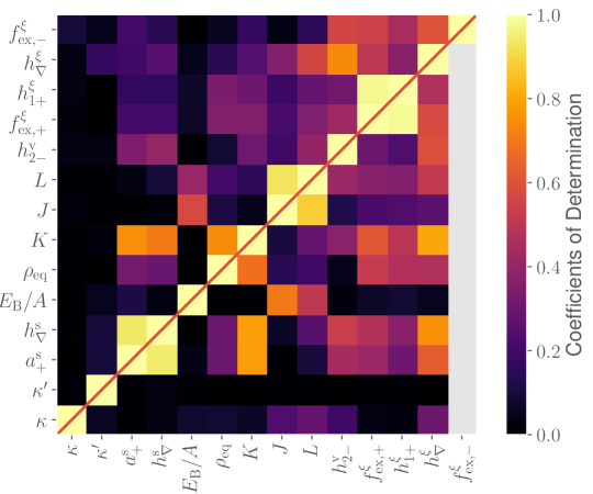
Figure 3: Coefficients of determination $R_{\alpha\beta}^{2}$ for the 13D (lower triangle) and 14D (upper triangle) calibrations. The parameters are ordered to highlight their correlations.

The correlations between model parameters in the vicinity of our solution are quantified by the matrix of CoDs. Figure 3 visualizes the correlations for both the 13D and 14D calibrations. Considerable correlations exist for some groups of parameters, which show that the number of the degrees of freedom of the model is less than the number of parameters [44]. For example, strong correlations exist between the two surface parameters ($a^{\mathrm{s}}_{+},h^{\mathrm{s}}_{\nabla}$), between the two symmetry parameters ($J$,$L$), and between two pairing parameters ($f^{\xi}_{\mathrm{ex},+},h^{\xi}_{1+}$). Several somewhat smaller, but still strong, correlations also exist. For example, surface parameters and $K$ correlate because both have impact on nuclear radii. Binding energy and symmetry energy parameters correlate because of some long isotopic chains in the data pool. Practically uncorrelated are the two spin orbit parameters $\kappa$ and $\kappa^{\prime}$. All these correlations behave similarly in both calibration variants, and they appear also in other models [45]. Not surprisingly, however, some correlations differ with pairing parameters. For example, the 13D variant shows considerable correlation of $f^{\xi}_{\mathrm{ex},+},h^{\xi}_{1+}$ with surface parameters while the 14D variant has lost this correlation because of the introduction of the isovector pairing parameter $f^{\xi}_{\mathrm{ex},-}$. A similar reduction of correlations happens for the connection between pairing parameters and the group $K$, $\rho_{\mathrm{eq}}$. It is not uncommon for correlations to get reduced with new parameters because they remove a previously existing rigidity within a model [46, 47]. Although the new parameter $f_{\mathrm{ex},-}^{\xi}$ has most of its correlations within the group of pairing parameters, it is rather independent from them. Correlations with other model parameters are generally weak, except for $h^{v}_{2-}$, which is related to isovector density dependence.

4.3 Sensitivity analysis

Minimization of the objective function delivers the optimized parameter set $\hat{\bm{x}}$. Sensitivity analysis deals with the question of how the parameters change, $\tilde{x}_{\alpha}\longrightarrow\tilde{x}_{\alpha}+\delta\tilde{x}_{\alpha}$, if the data are varied by a small amount, $\tilde{d}_{i}\longrightarrow\tilde{d}_{i}+\delta\tilde{d}_{i}$. Note that we formulate the problem in terms of dimensionless data (3e) and dimensionless parameters (3i) to allow a seamless combined handling of different types of data and parameters. Following forward error analysis [48], we search for the solution $\hat{\bm{x}}+\delta\bm{x}$ to the optimization problem (3f) but with the modified dataset $\tilde{d}_{i}+\delta\tilde{d}_{i}$ and find

$$\delta\tilde{x}_{\alpha}^{(i)}=S_{\alpha i}\delta\tilde{d}_{i}\;,\;S_{\alpha i}=\frac{\left[(\hat{J}^{T}\hat{J})^{-1}\hat{J}^{T}\right]_{\alpha i}}{\hat{\sigma}_{\alpha}}.$$ (3k)

Equation (3k) establishes the connection to a parameter change for small perturbations $\delta\tilde{d}_{i}$, and can be expressed also as $S_{\alpha i}=\delta\tilde{x}_{\alpha}^{(i)}/\delta\tilde{d}_{i}$. In the following, we assume that all dimensionless data points are changed by the same amount $\delta\tilde{d}_{i}=\delta\tilde{d}=$ constant. Since (3k) is in the linear regime, changes $\delta\tilde{x}_{\alpha}^{(i)}$ are proportional to $\delta\tilde{d}$. We are interested in the relative effects, and thus the actual value of $\delta\tilde{d}$ is unimportant once the approximation in (3k) is employed.

From the (dimensionless) sensitivity matrix we build the real-valued, positive number $\mathcal{S}_{\alpha i}=|S_{\alpha i}|^{2}$ as a measure for the impact of data point $\tilde{d}_{i}$ on parameter $\tilde{x}_{\alpha}$. The matrix of sensitivities $\mathcal{S}_{\alpha i}$ carries a huge amount of information about the calibrated model. First, we look at the sensitivity for observable classes $C$ of energies, radii, and so on. Instead of asking, for example, what is the impact of the energy of ²⁰⁸Pb on a parameter $\tilde{x}_{\alpha}$, we ask now, what is the impact of all the energy entries. To that end, we build the sum of the detailed $\mathcal{S}_{\alpha i}$ over the data $i$ in class $C$:

$$\mathcal{S}_{\alpha}^{(C)}=\sum_{i\in C}\mathcal{S}_{\alpha i}.$$ (3l)

The relative sensitivity per class is given by

$$s_{\alpha}^{(C)}=\frac{\mathcal{S}_{\alpha}^{(C)}}{\sum_{c}\mathcal{S}_{\alpha}^{(c)}}$$ (3m)

and does not depend on the choice of $\delta\tilde{d}$ as desired.

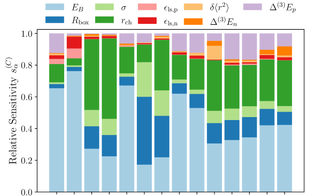
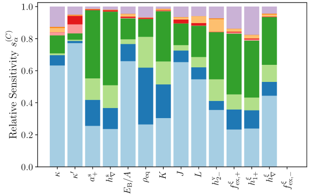
Figure 4: Relative sensitivities per data class (3m) for the model parameters of the 13D Fy($\Delta r$,13D) (bottom) and 14D Fy($\Delta r$,14D) (top) EDFs. The data classes are represented by colors as indicated. The $\delta\langle r^{2}\rangle$ represent the isotopic radius² differences and the $\Delta^{(3)}E$ the odd-even staggerings of energies.

Figure 4 shows the relative sensitivities for the 13D and 14D calibration variants. The patterns are similar to those already seen for Skyrme models [27]. The parameters $E_{\rm B}/A$, $J$, and $L$ are most influenced by the binding energy data while $\rho_{\mathrm{eq}}$, $K$, and surface parameters $a_{+}^{s}$ and $h_{\nabla}^{s}$ are more sensitive to surface data $R_{\rm box},\sigma$, and $r_{\rm ch}$. The spin orbit parameters $\kappa$ and $\kappa^{\prime}$ are dominated by energy information while the data on the spin-orbit splitting, $\epsilon_{\mathrm{ls}}$, play a surprisingly small role. The pairing parameters $f^{\xi}_{\mathrm{ex},\pm},h^{\xi}_{1+},$ and $h^{\xi}_{\nabla}$ are impacted primarily by binding energies and surface data. The differential data, $\delta\langle r^{2}\rangle$ and $\Delta^{(3)}E$, are important for the determination of the pairing functional in the 14D variant, especially for $h^{\xi}_{1+}$.

The effect of one data point $\tilde{d}_{i}$ on the model parameters also provides interesting information. To this end, we add up the detailed sensitivities over all parameters, coming to the total impact of a data point $\tilde{d}_{i}$ as $\sum_{\alpha}\mathcal{S}_{\alpha i}$. To render the different data points comparable, we use a constant change $\delta\tilde{d}_{i}=\delta\tilde{d}=1$. To see the effect of another value $\delta\tilde{d}$, we simply scale the resulting total impact by this value.

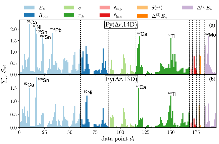
Figure 5: Total impact of a data point $i$ on the parameters of the Fy($\Delta r$,14D) (a) and Fy($\Delta r$,13D) (b) EDFs. The data classes are separated by dashed vertical lines as in figure 1. The data points having the largest impact on calibration results are indicated.

Figure 5 shows the result of our sensitivity study. Note that the absolute values are unimportant here; the main information is contained in the relative distribution. In general, the calibration dataset is fairly balanced, with only several data points showing significant variations. The most pronounced peaks in the 14D variant are the binding energies of ⁵²Ca, ⁶⁸Ni, ¹⁰⁰Sn, and ²¹⁴Pb; the charge radii of ⁴²Ca and ⁵⁰Ti; and the proton 3-point binding energy difference for ⁹²Mo. For the 13D EDF, the importance of $E_{\rm B}$ for ¹³²Sn and ²¹⁴Pb and $\Delta^{(3)}E_{p}$ for ⁹²Mo is reduced. Furthermore, we note that the sensitivities for $\Delta^{(3)}E_{n}$, and even more so for $\Delta^{(3)}E_{p}$, are generally larger for 14D. These results are related to the fact that 14D has more leeway in the pairing functional. The results show, first, that sensitivity not only is a property of data but also is intimately connected with the form of the functional and, second, that more versatility in the functional often leads to more sensitivity.

5 Predictions

5.1 Impact of isovector pairing on pairing gaps

At the end of the discussion of table 3, we saw that the density-independent proton pairing strength is increased when going from 13D to 14D while the neutron strength remains almost the same. This should be visible from typical calculated pairing observables (e.g., the proton and neutron pairing gaps).

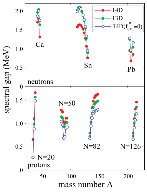
Figure 6: Comparison of the spectral pairing gaps [49], $\overline{\Delta}_{\tau_{3}}=\sum_{\alpha\in{\tau_{3}}}\Delta_{\alpha}u_{\alpha}v_{\alpha}/\sum_{\alpha\in{\tau_{3}}}u_{\alpha}v_{\alpha}$, for (top) neutrons and (bottom) protons obtained with Fy($\Delta r$,14D) and Fy($\Delta r$,13D) and also with Fy($\Delta r$,14D) with $f_{\mathrm{ex},-}^{\xi}=0$.

Figure 6 compares the spectral pairing gaps [49] obtained with Fy($\Delta r$,14D) and Fy($\Delta r$,13D) and also with Fy($\Delta r$,14D) assuming $f_{\mathrm{ex},-}^{\xi}=0$. As expected, when going from 13D to 14D, proton gaps increase. However, the neutron gaps decrease substantially from 13D to 14D while the density-independent pairing strengths are practically the same in both variants. This result indicates that the rearrangement of all parameters, in particular those defining the density-dependent part of the pairing functional, strongly impact spectral pairing gaps. As a counter check, we also considered a variation of 14D with the only change that we fix $f^{\xi}_{\mathrm{ex},-}=0$. The difference between the results of the 13D variant and those of the 14D variant having $f^{\xi}_{\mathrm{ex},-}=0$ indicates the impact of readjustment of 13 parameters of 13D in the 14D results.

5.2 Predictions of observables along isotopic chains

As discussed earlier, the additional isovector degree of freedom in Fy($\Delta r$,14D) allows a better adjustment to data, particularly with regard to isovector trends. This raises the question of how the two parameterizations perform in extrapolations outside the pool of the training dataset $\cal D$. We look at this now in terms of four long isotopic chains of spherical semi-magic nuclei: Ca, Sn, and Pb. We also study the deformed chain of Yb isotopes.

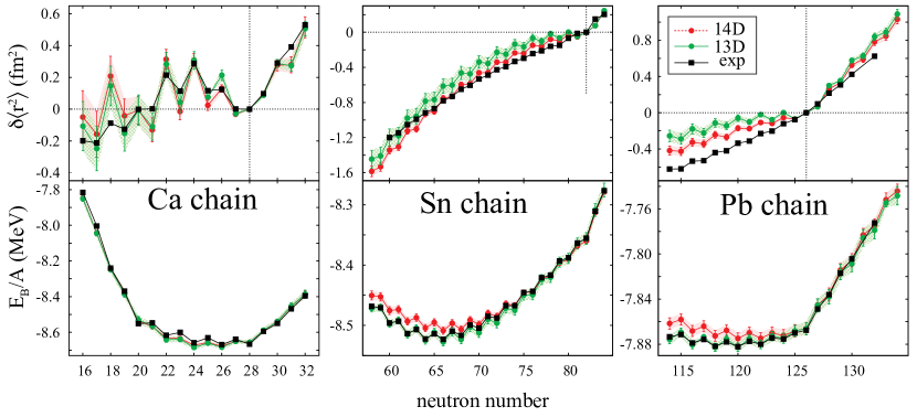
Figure 7: Comparison of the Fy($\Delta r$,13D) and Fy($\Delta r$,14D) results for $\langle\delta r^{2}\rangle$ (top) and $E_{\rm B}/A$ (bottom) with experiment for three semi-magic isotopic chains: Ca (left), Sn (middle), and Pb (right). The statistical uncertainties of the predictions [36] are shown as error bars and error bands. All even-even nuclei in these chains are spherical, and calculations were done with the axial DFT solver SkyAx. The differential radii are shown relative to ⁴⁸Ca, ¹³²Sn, and ²⁰⁸Pb. Experimental binding energies are from [50]. Experimental radii are from [38, 51] (Ca), [14] (Sn), and [52] (Pb).

Figure 7 shows binding energies and differential radii along the Ca, Sn, and Pb chains. As expected, binding energies are well described for the fit nuclei, which are the even-even isotopes ⁴⁰Ca-⁴⁸Ca, Sn with $N\geq 72$, and Pb with $N\geq 122$. The agreement persists along the whole Ca chain. Differences develop at the lower ends of the Sn and Pb chains where 13D remains close to data and 14D becomes slightly less bound. This happens because 14D produces less pairing for the proton-rich isotopes than does 13D, a consequence of the isovector pairing. This should not be taken too seriously because the low-$N$ isotopes are becoming increasingly deformation-soft and thus prone to ground-state correlations.

The differential charge radii are shown the upper panels in figure 7. This observable is more sensitive to isovector properties than the absolute charge radii. The trends in the Ca chain are similar for 13D and 14D. Both tend to slightly overestimate the odd-even staggering of radii. This is a feature already known from earlier Fayans EDF studies [9, 10]. Note, however, that the odd-even charge radius staggering had not been included in the dataset $\cal D$. The overall trend of differential radii for Sn and Pb is similar to that for energies, with an increasing difference between 13D and 14D toward low $N$. For both chains, the Fy($\Delta r$,14D) results stay closer to data. We note that the charge-radius kink at ²⁰⁸Pb is heavily influenced by the pairing and surface effects [53, 12].

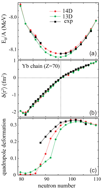
Figure 8: Comparison of the Fy($\Delta r$,13D) and Fy($\Delta r$,14D) results with experiment (where available) for the chain of Yb isotopes ($Z=70$). Since most of these isotopes are deformed, calculations were performed with the axial DFT solver SkyAx. (a) Total binding energy per particle. (b) Differential radii relative to ¹⁶⁶Yb. (c) Proton quadrupole deformations. Binding energies and deformations are calculated for even-even isotopes only. Experimental values are taken from [50] (binding energies), [52] (charge radii), and [54] (deformations).

Our calibration dataset ${\cal D}$ consists of data on spherical nuclei. It is thus interesting to look at the performance of Fy($\Delta r$,13D) and Fy($\Delta r$,14D) for well-deformed nuclei. Figure 8 shows binding energies, differential radii, and proton quadrupole deformations along the chain of Yb isotopes containing many deformed nuclei. For deformed systems, we augment the binding energies by a rotational energy correction approximating the angular momentum projection results as outlined in [55, 56]. This correction vanishes for spherical nuclei as discussed earlier. The calculated binding energies agree with the data, especially near the spherical ¹⁵²Yb and for the well-deformed heavier isotopes. Small differences are seen in the transitional region. As in our previous studies [57, 23], the description of differential radii is excellent. The proton quadrupole deformations $\beta_{2,p}$ show a transition from spherical shapes near the semi-magic ¹⁵²Yb to well-deformed isotopes for $N>95$. We note that experimental $\beta_{2}$ deformations deduced from $B(E2)$ values include zero-point quadrupole fluctuations from ground-state vibrations. The latter are particularly large in transitional nuclei. A detailed comparison with data would require accounting for these fluctuations.

Summarizing this section, the Fayans functionals Fy($\Delta r$,13D) and Fy($\Delta r$,14D) calibrated in this work perform well on the testing set of observables for spherical and deformed nuclei. In general the 14D model performs slightly better, especially for charge radii.

6 Conclusions

In previous work [31] we studied the performance of optimization-based training algorithms in the context of computationally expensive nuclear physics models based on modest calibration datasets. We concluded that the POUNDerS algorithm, within a budget of function evaluations, is extremely robust in the context of nuclear EDF calibration.

In this work we employed POUNDerS to carry out parameter estimation of two Fayans functionals, Fy($\Delta r$,13D) and Fy($\Delta r$,14D). The latter functional accounts for different strengths of proton and neutron pairing, which generally improved the agreement of the model with ground-state properties.

We carried out sensitivity analysis of these 13D and 14D parameterizations and studied the sensitivity of model parameters to changes in data points ${d}_{i}$. We concluded that the binding energy of ⁵²Ca, ⁶⁸Ni, ¹⁰⁰Sn, and ²¹⁴Pb, the charge radii of of ⁴²Ca and ⁵⁰Ti, and the proton 3-point binding energy difference for ⁹²Mo have the most pronounced impact on Fy($\Delta r$,14D).

In future work we will generalize the surface Fayans functional by adding the isovector surface term. Such an extension is important for systematic calculations of deformed nuclei and fission [58, 28]. New calibration datasets will include data on deformed nuclei, including fission isomers.

Appendix A Local densities and currents in detail

The Fayans EDF, as the Skyrme EDF, is formulated in terms of local densities and currents.

$$\begin{array}[]{rclcl}\hline\cr\mbox{Symbol}&&\mbox{Expression}&&\mbox{Name}\\[5.0pt] \rho_{\tau_{3}}&=&\displaystyle\sum_{\alpha\in{\tau_{3}}}v_{\alpha}^{2}|\varphi_{\alpha}|^{2}&&\mbox{density}\\ \bm{s}_{\tau_{3}}&=&\displaystyle\sum_{\alpha\in{\tau_{3}}}v_{\alpha}^{2}\varphi^{+}_{\alpha}\hat{\bm{\sigma}}\varphi^{\mbox{}}_{\alpha}&&\mbox{spin density}\\ \bm{j}_{\tau_{3}}&=&\displaystyle\Im{m}\left\{\sum_{\alpha\in{\tau_{3}}}v_{\alpha}^{2}\varphi^{+}_{\alpha}\bm{\nabla}\varphi^{\mbox{}}_{\alpha}\right\}&&\mbox{current}\\ \bm{J}_{\tau_{3}}&=&\displaystyle-\mathrm{i}\sum_{\alpha\in{\tau_{3}}}v_{\alpha}^{2}\varphi_{\alpha}^{+}\bm{\nabla}\times\hat{\bm{\sigma}}\varphi^{\mbox{}}_{\alpha}&&\mbox{spin-orbit density}\\ \tau_{\tau_{3}}&=&\displaystyle\sum_{\alpha\in{\tau_{3}}}v_{\alpha}^{2}|\bm{\nabla}\varphi_{\alpha}|^{2}&&\mbox{kinetic-energy density}\\ \bm{\tau}_{\tau_{3}}&=&\displaystyle-\mathrm{i}\sum_{\alpha\in{\tau_{3}}}v_{\alpha}^{2}\bm{\nabla}\varphi_{\alpha}^{+}\cdot\bm{\nabla}\,\hat{\bm{\sigma}}\varphi^{\mbox{}}_{\alpha}&&\mbox{kinetic spin-density}\\[12.0pt] \xi_{\tau_{3}}&=&\displaystyle\sum_{\alpha\in{\tau_{3}},\alpha>0}f_{\alpha}u_{\alpha}v_{\alpha}|\varphi_{\alpha}|^{2}&&\mbox{pairing density}\\[5.0pt] \hline\cr\end{array}$$ (3n)

In this equation, $v_{\alpha}$ and $u_{\alpha}$ are the standard BCS (or canonical HFB) amplitudes. The phase-space weight $f_{\alpha}$ provides a smooth cutoff of the space of single-particle states included in pairing. All of the above expressions are local quantities that depend on the position vector $\bm{r}$ and refer to the local wave function components $\varphi_{\alpha}=\varphi_{\alpha}(\bm{r})$. The pairing density (3n) is restricted to $\alpha>0$, which stands for states with positive azimuthal angular momenta (the other half with $\alpha<0$ are the pairing conjugate states).

For the pairing cutoff, we use a soft cutoff with the profile [33]

$$f_{\alpha}=\big{(}1+\exp{\left((\varepsilon_{\alpha}-(\epsilon_{\mathrm{F},q_{\alpha}}+\epsilon_{\mathrm{cut}}))/\Delta\epsilon\right)}\big{)}^{-1},$$ (3o)

where $\varepsilon_{\alpha}$ are the single-particle energies, $\epsilon_{\mathrm{cut}}$ marks the cutoff band, and $\Delta\epsilon=\epsilon_{\mathrm{cut}}/10$ is its width. We use a dynamical setting of the pairing band where $\epsilon_{\mathrm{cut}}$ is adjusted such that a fixed number of nucleons $N_{q}+\eta_{\mathrm{cut}}N_{q}^{2/3}$ is included [49], here with $\eta_{\mathrm{cut}}=5$ as in [9].

Appendix B Nuclear matter properties

Bulk properties of symmetric nuclear matter at equilibrium, called nuclear matter properties (NMPs), are often used to characterize the properties of a model, or functional respectively. A starting point for the definition of NMPs is the binding energy per nucleon in the symmetric nuclear matter

$$E_{\rm B}/A=E(\rho_{0},\rho_{1},\tau_{0},\tau_{1})/A=\frac{\mathcal{E}_{\mathrm{Fy}}^{\mathrm{v}}}{\rho_{0}}\;,$$ (3p)

which depends uniquely on the volume term (3b) of the functional. Variation with respect to Kohn–Sham wave functions establishes a relation $\tau_{t}=\tau_{t}(\rho_{0},\rho_{1})$ between kinetic densities $\tau_{t}$ and densities $\rho_{t}$. This yields the commonly used binding energy at equilibrium, $E_{\rm B}/A\left[\rho_{0},\rho_{1},\tau_{0}(\rho_{0},\rho_{1}),\tau_{1}(\rho_{0},\rho_{1})\right]$, as a function of the densities $\rho_{t}$ alone.

Table 4: Definitions of NMPs used in this work. All derivatives are to be taken at the equilibrium point corresponding to the equilibrium density $\rho_{\mathrm{eq}}$.

binding energy:	$\displaystyle\frac{{E_{\rm B}}}{A}$	=	$\displaystyle\displaystyle\frac{{E_{\rm B}}}{A}\Big{|}_{\mathrm{eq}}$
equilibrium density:	$\displaystyle\rho_{0,\rm{eq}}$	$\leftrightarrow$	$\partial_{\rho_{0}}\frac{{E_{\rm B}}}{A}=0$
incompressibility:	$K_{\infty}$	=	$\displaystyle 9\,\rho_{0}^{2}\,\frac{d^{2}}{d\rho_{0}^{2}}\,\frac{{E_{\rm B}}}{A}\Big{|}_{\mathrm{eq}}$
symmetry energy:	$a_{\mathrm{sym}}$	=	$\displaystyle\frac{1}{2}\rho_{0}^{2}\frac{d^{2}}{d\rho_{1}^{2}}\frac{{{}_{\rm B}}}{A}\bigg{|}_{\mathrm{eq}}\equiv J$
slope of $a_{\mathrm{sym}}$:	$L$	=	$\displaystyle 3\rho_{0}\frac{da_{\mathrm{sym}}}{d\rho_{0}}\bigg{|}_{\mathrm{eq}}$

Table 4 lists the NMPs discussed in this work. We consider $\tau_{t}$ as independent variables for the purpose of a formally compact definition of the effective mass. Static properties are deduced from the binding energy at equilibrium, which depends on $\rho_{0}$ only. This is indicated by using the total derivatives for $K_{\infty}$, $a_{\mathrm{sym}}$, and $L$. The slope of the symmetry energy $L$ parameterizes the density dependence of $a_{\mathrm{sym}}$.

All these NMPs depend on the volume parameters of the Fayans functional through (3p). There are six volume parameters in $E_{\rm B}/{A}|_{\mathrm{eq}}$ and five NMPs. We use the NMPs to express five of the volume parameters. ${h_{2-}^{\mathrm{v}}}$ is the sole remaining volume parameter.

Appendix C Input data in detail

Table 5: Calibration data Part I: bulk data along isotopic chains.

A	Z	$E_{\rm B}$	$\Delta E_{\rm B}$	$R_{\mathrm{box}}$	$\Delta R_{\mathrm{box}}$	$\sigma$	$\Delta\sigma$	$r_{\mathrm{ch}}$	$\Delta r_{\mathrm{ch}}$
		MeV		fm		fm		fm
16	8	-127.620	4	2.777	0.08	0.839	0.08	2.701	0.04
36	20	-281.360	2					3.450	0.18
38	20	-313.122	2					3.466	0.10
40	20	-342.051	3	3.845	0.04	0.978	0.04	3.478	0.02
42	20	-361.895	2	3.876	0.04	0.999	0.04	3.513	0.04
44	20	-380.960	2	3.912	0.04	0.975	0.04	3.523	0.04
46	20	-398.769	2					3.502	0.02
48	20	-415.990	1	3.964	0.04	0.881	0.04	3.479	0.04
50	20	-427.491	1					3.523	0.18
52	20	-436.571	1					3.5531	0.18
58	26							3.7745	0.18
56	28	-483.990	5					3.750	0.18
58	28	-506.500	5	4.364	0.04			3.776	0.10
60	28	-526.842	5	4.396	0.04	0.926	0.20	3.818	0.10
62	28	-545.258	5	4.438	0.04	0.937	0.20	3.848	0.10
64	28	-561.755	5	4.486	0.04	0.916	0.08	3.868	0.10
68	28	-590.430	1
100	50	-825.800	2
108	50							4.563	0.04
112	50			5.477	0.12	0.963	0.36	4.596	0.18
114	50			5.509	0.12	0.948	0.36	4.610	0.18
116	50			5.541	0.12	0.945	0.36	4.626	0.18
118	50			5.571	0.08	0.931	0.08	4.640	0.02
120	50			5.591	0.04			4.652	0.02
122	50	-1035.530	3	5.628	0.04	0.895	0.04	4.663	0.02
124	50	-1050.000	3	5.640	0.04	0.908	0.04	4.674	0.02
126	50	-1063.890	2
128	50	-1077.350	2
130	50	-1090.400	1
132	50	-1102.900	1
134	50	-1109.080	1
198	82	-1560.020	9					5.450	0.04
200	82	-1576.370	9					5.459	0.02
202	82	-1592.203	9					5.474	0.02
204	82	-1607.521	2	6.749	0.04	0.918	0.04	5.483	0.02
206	82	-1622.340	1	6.766	0.04	0.921	0.04	5.494	0.02
208	82	-1636.446	1	6.776	0.04	0.913	0.04	5.504	0.02
210	82	-1645.567	1					5.523	0.02
212	82	-1654.525	1					5.542	0.02
214	82	-1663.299	1					5.559	0.02

Table 6: Calibration data Part II. Similar as in table 5, but for nuclei along isotonic chains.

A	Z	$E_{\rm B}$	$\Delta E_{\rm B}$	$R_{\mathrm{box}}$	$\Delta R_{\mathrm{box}}$	$\sigma$	$\Delta\sigma$	$r_{\mathrm{ch}}$	$\Delta r_{\mathrm{ch}}$
		MeV		fm		fm		fm
34	14	-283.429	2
36	16	-308.714	2	3.577	0.16	0.994	0.16	3.299	0.02
38	18	-327.343	2					3.404	0.02
50	22	-437.780	2	4.051	0.04	0.947	0.08	3.570	0.02
52	24			4.173	0.04	0.924	0.16	3.642	0.04
54	26			4.258	0.04	0.900	0.16	3.693	0.04
86	36	-749.235	2					4.184	0.02
88	38	-768.467	1	4.994	0.04	0.923	0.04	4.220	0.02
90	40	-783.893	1	5.040	0.04	0.957	0.04	4.269	0.02
92	42	-796.508	1	5.104	0.04	0.950	0.04	4.315	0.02
94	44	-806.849	2
96	46	-815.034	2
98	48	-821.064	2
134	52	-1123.270	1
136	54	-1141.880	1					4.791	0.02
138	56	-1158.300	1	5.868	0.08	0.900	0.08	4.834	0.02
140	58	-1172.700	1					4.877	0.02
142	60	-1185.150	2	5.876	0.12	0.989	0.12	4.915	0.02
144	62	-1195.740	2					4.960	0.02
146	64	-1204.440	2					4.984	0.02
148	66	-1210.750	2					5.046	0.04
150	68	-1215.330	2					5.076	0.04
152	70	-1218.390	2
206	80	-1621.060	1					5.485	0.02
210	84	-1645.230	1					5.534	0.02
212	86	-1652.510	1					5.555	0.02
214	88	-1658.330	1					5.571	0.02
216	90	-1662.700	1
218	92	-1665.650	1

Table 7: Calibration data Part III: spin-orbit splittings (upper block) and adopted errors of 3-point binding energy differences (lower block) for neutrons $\Delta^{(3)}_{n}E(Z,N)=\frac{1}{2}(E_{\rm B}(Z,N\!+\!2)-2E_{\rm B}(Z,N)+E_{\rm B}(Z,N\!-\!2))$ and for protons $\Delta^{(3)}_{p}E(Z,N)=\frac{1}{2}(E_{\rm B}(Z\!+\!2,N)-2E_{\rm B}(Z,N)+E_{\rm B}(Z\!-\!2,N))$. All quantities are in MeV.

$A$	$Z$	Level	$\varepsilon_{ls,p}$	$\Delta\varepsilon_{ls,p}$	Level	$\varepsilon_{ls,n}$	$\Delta\varepsilon_{ls,n}$
16	8	1p	6.30	60%	1p	6.10	60%
132	50	2p	1.35	20%	2d	1.65	20%
208	82	2d	1.42	20%	1f	0.90	20%
					3p	1.77	40%

$\Delta^{(3)}_{n}E$				$\Delta^{(3)}_{p}E$
$A$	$Z$	Data	Error	$A$	$Z$	Data	Error
44	20	0.628	0.24	36	16	3.328	0.36
118	50	0.330	0.36	88	38	1.903	0.36
120	50	0.300	0.36	90	40	1.4055	0.24
122	50	0.260	0.24	92	42	1.137	0.12
124	50	0.290	0.24	94	44	1.078	0.24
				136	54	1.095	0.24
				138	56	1.010	0.24
				140	58	0.975	0.24
				142	60	0.930	0.24
				214	88	0.725	0.24
				216	90	0.710	0.24

Table 8: Calibration data Part IV: differential charge radii $\delta\langle r^{2}\rangle^{A,A^{\prime}}=\langle r^{2}_{\rm ch}\rangle^{A}-\langle r^{2}_{\rm ch}\rangle^{A^{\prime}}$ (in fm²).

$\delta\langle r^{2}\rangle^{A,A^{\prime}}\;$ A A’ Z Data Error 48 40 20 0.006957 0.008 48 44 20 -0.308088 0.008 52 48 20 0.52107861 0.020

Tables 5, 6, 7, and 8 show the detailed calibration data $\cal D$ together with their adopted error.

References

The submitted manuscript has been created by UChicago Argonne, LLC, Operator of Argonne National Laboratory (“Argonne”). Argonne, a U.S. Department of Energy Office of Science laboratory, is operated under Contract No. DE-AC02-06CH11357. The U.S. Government retains for itself, and others acting on its behalf, a paid-up nonexclusive, irrevocable worldwide license in said article to reproduce, prepare derivative works, distribute copies to the public, and perform publicly and display publicly, by or on behalf of the Government. The Department of Energy will provide public access to these results of federally sponsored research in accordance with the DOE Public Access Plan. http://energy.gov/downloads/doe-public-access-plan.

References

- [1] Bender M, Heenen P H and Reinhard P G 2003 Rev. Mod. Phys. 75 121–180 URL https://link.aps.org/doi/10.1103/RevModPhys.75.121
- [2] Duguet T 2014 The nuclear energy density functional formalism Euroschool Exot. Beams, Vol. IV vol 879 ed Scheidenberger C and Pfützner M (Springer Berlin Heidelberg) chap 7, pp 293–350 ISBN 978-3-642-45140-9 URL http://link.springer.com/10.1007/978-3-642-45141-6http://link.springer.com/10.1007/978-3-642-45141-6_7
- [3] Schunck N 2019 Energy Density Functional Methods for Atomic Nuclei (IOP Publishing) ISBN 978-0-7503-1422-0 URL https://iopscience.iop.org/book/978-0-7503-1422-0
- [4] Neufcourt L, Cao Y, Giuliani S A, Nazarewicz W, Olsen E and Tarasov O B 2020 Phys. Rev. C 101(4) 044307 URL https://link.aps.org/doi/10.1103/PhysRevC.101.044307
- [5] Fayans S, Tolokonnikov S, Trykov E and Zawischa D 1994 Phys. Lett. B 338 1–6 ISSN 0370-2693 URL http://www.sciencedirect.com/science/article/pii/037026939491334X
- [6] Fayans S A 1998 J. Exp. Theor. Phys. Lett. 68 169–174 URL https://doi.org/10.1134/1.567841
- [7] Fayans S, Tolokonnikov S, Trykov E and Zawischa D 2000 Nucl. Phys. A 676 49 URL https://www.sciencedirect.com/science/article/abs/pii/S0375947400001925
- [8] Tolokonnikov S V, Borzov I N, Kortelainen M, Lutostansky Y S and Saperstein E E 2015 J. Phys. G 42 075102 URL https://dx.doi.org/10.1088/0954-3899/42/7/075102
- [9] Reinhard P G and Nazarewicz W 2017 Phys. Rev. C 95(6) 064328 URL https://link.aps.org/doi/10.1103/PhysRevC.95.064328
- [10] Miller A J, Minamisono K, Klose A, Garand D, Kujawa C, Lantis J D, Liu Y, Maaß B, Mantica P F, Nazarewicz W, Nörtershäuser W, Pineda S V, Reinhard P G, Rossi D M, Sommer F, Sumithrarachchi C, Teigelhöfer A and Watkins J 2019 Nat. Phys. 15 432–436 URL https://www.nature.com/articles/s41567-019-0416-9
- [11] Hammen M, Nörtershäuser W, Balabanski D L, Bissell M L, Blaum K, Budinčević I, Cheal B, Flanagan K T, Frömmgen N, Georgiev G, Geppert C, Kowalska M, Kreim K, Krieger A, Nazarewicz W, Neugart R, Neyens G, Papuga J, Reinhard P G, Rajabali M M, Schmidt S and Yordanov D T 2018 Phys. Rev. Lett. 121(10) 102501 URL https://link.aps.org/doi/10.1103/PhysRevLett.121.102501
- [12] Gorges C et al. 2019 Phys. Rev. Lett. 122(19) 192502 URL https://journals.aps.org/prl/abstract/10.1103/PhysRevLett.122.192502
- [13] de Groote R, Billowes J, Binnersley C, Bissell M, Cocolios T, Day Goodacre T, Farooq-Smith G, Fedorov D, Flanagan K, Franchoo S, Garcia Ruiz R, Gins W, Holt J, Koszorus A, Miyagi T, Nazarewicz W, Neyens G, Reinhard P and Yang X 2020 Nat. Phys. 16 620–624 URL https://www.nature.com/articles/s41567-020-0868-y
- [14] Yordanov D T, Rodríguez L V, Balabanski D L, Bieroń J, Bissell M L, Blaum K, Cheal B, Ekman J, Gaigalas G, Garcia Ruiz R F, Georgiev G, Gins W, Godefroid M R, Gorges C, Harman Z, Heylen H, Jönsson P, Kanellakopoulos A, Kaufmann S, Keitel C H, Lagaki V, Lechner S, Maaß B, Malbrunot-Ettenauer S, Nazarewicz W, Neugart R, Neyens G, Nörtershäuser W, Oreshkina N S, Papoulia A, Pyykkö P, Reinhard P G, Sailer S, Sánchez R, Schiffmann S, Schmidt S, Wehner L, Wraith C, Xie L, Xu Z and Yang X 2020 Commun. Phys. 3 107 URL https://doi.org/10.1038/s42005-020-0348-9
- [15] Borzov I N and Tolokonnikov S V 2020 Phys. Atom. Nucl. 83 828–840 URL https://doi.org/10.1134/S1063778820060101
- [16] Koszorús, Yang X F, Jiang W G, Novario S J, Bai S W, Billowes J, Binnersley C L, Bissell M L, Cocolios T E, Cooper B S, de Groote R P, Ekström A, Flanagan K T, Forssén C, Franchoo S, Ruiz R F, Gustafsson F P, Hagen G, Jansen G R, Kanellakopoulos A, Kortelainen M, Nazarewicz W, Neyens G, Papenbrock T, Reinhard P G, Ricketts C M, Sahoo B K, Vernon A R and Wilkins S G 2021 Nat. Phys. 17 439–443 ISSN 17452481 URL https://doi.org/10.1038/s41567-020-01136-5
- [17] Reponen M, de Groote R P, Al Ayoubi L, Beliuskina O, Bissell M L, Campbell P, Cañete L, Cheal B, Chrysalidis K, Delafosse C, de Roubin A, Devlin C S, Eronen T, Garcia Ruiz R F, Geldhof S, Gins W, Hukkanen M, Imgram P, Kankainen A, Kortelainen M, Koszorús Á, Kujanpää S, Mathieson R, Nesterenko D A, Pohjalainen I, Vilén M, Zadvornaya A and Moore I D 2021 Nat. Commun. 12 4596 URL https://doi.org/10.1038/s41467-021-24888-x
- [18] Reinhard P G and Nazarewicz W 2022 Phys. Rev. C 105(2) L021301 URL https://link.aps.org/doi/10.1103/PhysRevC.105.L021301
- [19] Kortelainen M, Sun Z, Hagen G, Nazarewicz W, Papenbrock T and Reinhard P G 2022 Phys. Rev. C 105(2) L021303 URL https://link.aps.org/doi/10.1103/PhysRevC.105.L021303
- [20] Malbrunot-Ettenauer S, Kaufmann S, Bacca S, Barbieri C, Billowes J, Bissell M L, Blaum K, Cheal B, Duguet T, Ruiz R F G, Gins W, Gorges C, Hagen G, Heylen H, Holt J D, Jansen G R, Kanellakopoulos A, Kortelainen M, Miyagi T, Navrátil P, Nazarewicz W, Neugart R, Neyens G, Nörtershäuser W, Novario S J, Papenbrock T, Ratajczyk T, Reinhard P G, Rodríguez L V, Sánchez R, Sailer S, Schwenk A, Simonis J, Somà V, Stroberg S R, Wehner L, Wraith C, Xie L, Xu Z Y, Yang X F and Yordanov D T 2022 Phys. Rev. Lett. 128(2) 022502 URL https://link.aps.org/doi/10.1103/PhysRevLett.128.022502
- [21] Geldhof S, Kortelainen M, Beliuskina O, Campbell P, Caceres L, Cañete L, Cheal B, Chrysalidis K, Devlin C S, de Groote R P, de Roubin A, Eronen T, Ge Z, Gins W, Koszorus A, Kujanpää S, Nesterenko D, Ortiz-Cortes A, Pohjalainen I, Moore I D, Raggio A, Reponen M, Romero J and Sommer F 2022 Phys. Rev. Lett. 128(15) 152501 URL https://link.aps.org/doi/10.1103/PhysRevLett.128.152501
- [22] Sommer F, König K, Rossi D M, Everett N, Garand D, de Groote R P, Holt J D, Imgram P, Incorvati A, Kalman C, Klose A, Lantis J, Liu Y, Miller A J, Minamisono K, Miyagi T, Nazarewicz W, Nörtershäuser W, Pineda S V, Powel R, Reinhard P G, Renth L, Romero-Romero E, Roth R, Schwenk A, Sumithrarachchi C and Teigelhöfer A 2022 Phys. Rev. Lett. 129(13) 132501 URL https://link.aps.org/doi/10.1103/PhysRevLett.129.132501
- [23] Hur J, Aude Craik D P L, Counts I, Knyazev E, Caldwell L, Leung C, Pandey S, Berengut J C, Geddes A, Nazarewicz W, Reinhard P G, Kawasaki A, Jeon H, Jhe W and Vuletić V 2022 Phys. Rev. Lett. 128(16) 163201 URL https://link.aps.org/doi/10.1103/PhysRevLett.128.163201
- [24] König K, Fritzsche S, Hagen G, Holt J D, Klose A, Lantis J, Liu Y, Minamisono K, Miyagi T, Nazarewicz W, Papenbrock T, Pineda S V, Powel R and Reinhard P G 2023 Phys. Rev. Lett. 131(10) 102501 URL https://link.aps.org/doi/10.1103/PhysRevLett.131.102501
- [25] Bertsch G F, Bertulani C A, Nazarewicz W, Schunck N and Stoitsov M V 2009 Phys. Rev. C 79(3) 034306 URL https://link.aps.org/doi/10.1103/PhysRevC.79.034306
- [26] Karthein J et al. 2023 Nat. Phys. submitted
- [27] Kortelainen M, Lesinski T, Moré J J, Nazarewicz W, Sarich J, Schunck N, Stoitsov M V and Wild S M 2010 Phys. Rev. C 82 024313 URL https://link.aps.org/doi/10.1103/PhysRevC.82.024313
- [28] Kortelainen M, McDonnell J D, Nazarewicz W, Reinhard P G, Sarich J, Schunck N, Stoitsov M V and Wild S M 2012 Phys. Rev. C 85 024304 URL https://link.aps.org/doi/10.1103/PhysRevC.85.024304
- [29] Kortelainen M, McDonnell J D, Nazarewicz W, Olsen E, Reinhard P G, Sarich J, Schunck N, Wild S M, Davesne D, Erler J and Pastore A 2014 Phys. Rev. C 89 054314 URL https://journals.aps.org/prc/abstract/10.1103/PhysRevC.89.054314
- [30] McDonnell J D, Schunck N, Higdon D, Sarich J, Wild S M and Nazarewicz W 2015 Phys. Rev. Lett. 114 122501 URL https://link.aps.org/doi/10.1103/PhysRevLett.114.122501
- [31] Bollapragada R, Menickelly M, Nazarewicz W, O’Neal J, Reinhard P G and Wild S M 2021 Journal of Physics G: Nuclear and Particle Physics 48 024001 URL https://doi.org/10.1088/1361-6471/abd009
- [32] Reinhard P G 1991 Skyrme–Hartree–Fock calculations of the nuclear ground state Computational Nuclear Physics I - Nuclear Structure ed Langanke K, Koonin S and Maruhn J (Berlin: Springer) p 28 URL https://doi.org/10.1007/978-1-4613-9335-1
- [33] Krieger S J, Bonche P, Flocard H, Quentin P and Weiss M S 1990 Nucl. Phys. A 517 275 URL https://doi.org/10.1016/0375-9474(90)90035-K
- [34] Reinhard P G, Schuetrumpf B and Maruhn J 2021 Comp. Phys. Comm. 258 107603 URL https://doi.org/10.1016/j.cpc.2020.107603
- [35] Birge R T 1932 Phys. Rev. 40 207–227 URL https://doi.org/10.1103/PhysRev.40.207
- [36] Dobaczewski J, Nazarewicz W and Reinhard P G 2014 J. Phys. G 41 074001 URL https://iopscience.iop.org/article/10.1088/0954-3899/41/7/074001
- [37] Wild S M 2017 POUNDERS in TAO: Solving derivative-free nonlinear least squares problems with POUNDERS Advances and Trends in Optimization with Engineering Applications ed Terlaky T, Anjos M F and Ahmed S (SIAM) pp 529–539 URL https://doi.org/10.1137/1.9781611974683.ch40
- [38] Friedrich J and Vögler N 1982 Nucl. Phys. A 373 192–224 URL https://doi.org/10.1016/0375-9474(82)90147-6
- [39] Klüpfel P, Erler J, Reinhard P G and Maruhn J A 2008 Eur. Phys. J. A 37 343 URL https://doi.org/10.1140/epja/i2008-10633-3
- [40] Reinhard P G, Nazarewicz W and Garcia Ruiz R F 2020 Phys. Rev. C 101(2) 021301 URL https://doi.org/10.1103/PhysRevC.101.021301
- [41] Moré J J and Wild S M 2011 SIAM J. Sci. Comput. 33 1292–1314 URL https://doi.org/10.1137/100786125
- [42] Moré J J and Wild S M 2012 ACM Trans. Math. Softw. 38 19:1–19:21 URL https://dl.acm.org/doi/abs/10.1145/2168773.2168777
- [43] Moré J J and Wild S M 2014 J. Comput. Phys. 273 268–277 URL https://dl.acm.org/doi/10.1016/j.jcp.2014.04.056
- [44] Kejzlar V, Neufcourt L, Nazarewicz W and Reinhard P G 2020 Journal of Physics G: Nuclear and Particle Physics 47 094001 URL https://dx.doi.org/10.1088/1361-6471/ab907c
- [45] Erler J and Reinhard P G 2015 J. Phys. G 42 034026 URL http://dx.doi.org/10.1088/0954-3899/42/3/034026
- [46] Reinhard P G and Nazarewicz W 2010 Phys. Rev. C 81(5) 051303 URL https://link.aps.org/doi/10.1103/PhysRevC.81.051303
- [47] Reinhard P G, Roca-Maza X and Nazarewicz W 2022 Phys. Rev. Lett. 129(23) 232501 URL https://link.aps.org/doi/10.1103/PhysRevLett.129.232501
- [48] Björck Å 1996 Numerical Methods for Least Squares Problems (Society for Industrial and Applied Mathematics) URL https://epubs.siam.org/doi/abs/10.1137/1.9781611971484
- [49] Bender M, Rutz K, Reinhard P G and Maruhn J A 2000 Eur. Phys. J. A 8 59–75 URL https://doi.org/10.1007/s10050-000-4504-z
- [50] Audi G, Wapstra A and Thibault C 2003 Nucl. Phys. A 729(1) 337 URL https://doi.org/10.1016/j.nuclphysa.2003.11.003
- [51] Garcia Ruiz R F, Bissell M L, Blaum K, Ekström A, Frömmgen N, Hagen G, Hammen M, Hebeler K, Holt J D, Jansen G R, Kowalska M, Kreim K, Nazarewicz W, Neugart R, Neyens G, Nörtershäuser W, Papenbrock T, Papuga J, Schwenk A, Simonis J, Wendt K A and Yordanov D T 2016 Nat. Phys. 12 594 URL http://dx.doi.org/10.1038/nphys3645
- [52] Angeli I and Marinova K P 2013 At. Data Nucl. Data Tables 99 69 URL https://doi.org/10.1016/j.adt.2011.12.006
- [53] Reinhard P G and Flocard H 1995 Nucl. Phys. A 584 467 URL https://doi.org/10.1016/0375-9474(94)00770-N
- [54] Raman S, Nestor C W and Tikkanen P 2001 At. Data Nucl. Data Tables 78(1) 1 URL https://www.sciencedirect.com/science/article/pii/S0092640X01908587
- [55] Reinhard P G 1978 Z. Phys. A 285 93 URL https://doi.org/10.1007/BF01410231
- [56] Erler J, Klüpfel P and Reinhard P G 2011 J. Phys. G 38 033101 URL http://dx.doi.org/10.1088/0954-3899/38/3/033101
- [57] Reinhard P G and Nazarewicz W 2022 Phys. Rev. C 106(1) 014303 URL https://link.aps.org/doi/10.1103/PhysRevC.106.014303
- [58] Nikolov N, Schunck N, Nazarewicz W, Bender M and Pei J 2011 Phys. Rev. C 83(3) 034305 URL https://link.aps.org/doi/10.1103/PhysRevC.83.034305