Identifying probabilistic weather regimes targeted to a local-scale impact variable

Abstract

Weather regimes are recurrent and persistent large-scale atmospheric circulation patterns that modulate the occurrence of local impact variables such as extreme precipitation. In their capacity as mediators between long-range teleconnections and these local extremes, they have shown potential for improving sub-seasonal forecasting as well as long-term climate projections. However, existing methods for identifying weather regimes are not designed to capture the physical processes relevant to the impact variable in question while still representing the full atmospheric phase space. This paper introduces a novel probabilistic machine learning method, RMM-VAE, for identifying weather regimes targeted to a local-scale impact variable. Based on a variational autoencoder architecture, the method combines non-linear dimensionality reduction with a prediction task and probabilistic clustering in a coherent architecture. The new method is applied to identify circulation patterns over the Mediterranean region targeted to precipitation over Morocco and compared to three existing approaches, two established linear methods and another machine learning approach. The RMM-VAE method identifies regimes that are more predictive of the target variable compared to the two linear methods, and more robust and persistent compared to the alternative machine learning method, while also improving the reconstruction of the input space. The results demonstrate the potential benefit of the new method for use in various climate applications such as sub-seasonal forecasting, while also highlighting the trade-offs involved in targeted clustering.

Keywords weather regimes  $\cdot$ variational autoencoders  $\cdot$ Mediterranean precipitation  $\cdot$ extreme events

1 Introduction

1.1 Weather Regimes

Large-scale atmospheric circulation modulates the occurrence of regional extremes such as heavy precipitation and heat waves that cause devastating impacts on people and livelihoods across the planet. In a changing climate, preparing for these extreme events becomes even more important and requires both an understanding of their projected long-term changes to make well-informed and robust adaptation decisions (Lemos et al., 2012), as well as an improvement of their near-term prediction skill to support early-warning decisions (Coughlan de Perez et al., 2022). Low-frequency variability of the large-scale atmospheric circulation has been understood through different research methods and paradigms (Ghil and Robertson, 2002). One common approach is the identification of recurrent and persistent atmospheric states, so-called weather regimes, based on statistical dimensionality reduction and clustering of variables such as geopotential height data over the region of interest (Hannachi et al., 2017).

For many applications, weather regimes can be interpreted as discrete mediators between teleconnections in the climate system and regional impact variables (Cassou, 2008; Gonzalez et al., 2022). For example, large-scale atmospheric patterns such as weather regimes have been used to disentangle dynamic and thermodynamic components of climate change for extreme event attribution or quantify the role of atmospheric internal variability in observed trends (Cattiaux et al., 2010; Horton et al., 2015; Terray, 2021), or to statistically downscale climate models (Ailliot et al., 2009; Maraun et al., 2010). Moreover, weather regimes have been shown to improve the usability and skill of forecasts at sub-seasonal-to-seasonal timescales (Allen et al., 2021; Bloomfield et al., 2021), due to their interpretability, persistence, as well as teleconnections with the Madden-Julian Oscillation (Gadouali et al., 2020), the El-Niño Southern Oscillation (Lee et al., 2019), or stratospheric states (Charlton-Perez et al., 2018), although different teleconnections will be relevant for different regions and timescales.

Although weather regimes over the North Atlantic/European region are the most extensively studied (Michelangeli et al., 1995; Vautard, 1990), weather regimes over other regions such as the Mediterranean (Giuntoli et al., 2022; Mastrantonas et al., 2020), the Indian subcontinent (Neal et al., 2020) and North America (Lee et al., 2023; Straus et al., 2007) have also been analysed and used in applications such as sub-seasonal forecasting (Robertson et al., 2020).

1.2 Dimensionality reduction and clustering for identifying regimes

Weather regimes are commonly identified using a combination of dimensionality reduction and clustering methods. While the dimensionality reduction step projects the high-dimensional data into a lower-dimensional subspace, the clustering step subsequently identifies and assigns discrete regimes within this reduced space (Murphy, 2022).

Following Michelangeli et al. (1995), Principal Component Analysis (PCA, often referred to as Empirical Orthogonal Function analysis in atmospheric sciences (Hannachi et al., 2007)) and k-means have established themselves as common choices for dimensionality reduction and clustering respectively. The advantage of this combination of methods is that they are easy to compute, understand, and interpret. However, they are not inherently more physically meaningful than other statistical dimensionality reduction and clustering methods, and several critiques have been highlighted and alternatives proposed in the literature on weather regimes. The present discussion is focused on critical aspects relevant to the analysis in this paper; for a detailed overview of different methodologies, see Hannachi et al. (2017) and Feldstein and Franzke (2017). Figure 1 illustrates some of the possible choices discussed in the following.

In terms of dimensionality reduction methods, PCA can be explicitly determined as the solution of an eigenvalue equation thanks to its linear and non-probabilistic nature. However, the linear transformation applied is not necessarily physically meaningful (Jolliffe and Cadima, 2016) or optimal for encoding the underlying features of the data (Murphy, 2022). Furthermore, a probabilistic method such as factor analysis should in general be preferred for the task of statistically identifying a subspace of limited and noisy high-dimensional data to better capture the uncertainty of the identified solution (Falkena et al., 2023). In terms of machine learning methods for dimensionality reduction, autoencoders can be seen as a non-linear extension of PCA implemented through an encoder and decoder neural network. Autoencoders are more efficient at encoding the input data compared to PCA but suffer from the fact that the identified latent space is not necessarily continuous which is an obstacle to subsequent clustering (Murphy, 2022). Variational autoencoders (VAEs) address the limitations of autoencoders by explicitly fitting a probabilistic model using Bayesian variational inference and thereby regularizing the dimensionality-reduced space, providing a both probabilistic and non-linear alternative to PCA (Kingma and Welling, 2013). Although the transformation into the dimensionality-reduced space can no longer be provided analytically, VAEs have been shown to provide an improved representation of the high-dimensional input space in lower dimensions in various machine learning applications, including the identification of weather regimes (Baldo and Locatelli, 2022).

In terms of clustering methods, k-means is susceptible to noise and loses information on transitional states between different weather regimes due to its hard cluster assignment (Falkena et al., 2023). Gaussian mixture models constitute a probabilistic alternative where clusters are fitted as probability distributions, and each data point is associated with probabilities of belonging to different clusters. K-means clustering also requires determining the number of clusters a priori, the most suitable method for which is not settled and has led to ongoing discussion in the literature (Dorrington and Strommen, 2020; Falkena et al., 2020; Feldstein and Franzke, 2017).

Figure 1: Illustration of selected methodological choices for dimensionality reduction and clustering based on Hannachi et al. (2017) and Murphy (2022). Methods highlighted in green refer to joint dimensionality reduction methods between two high-dimensional spaces. Also mentioned are clustering methods that incorporate temporal information into the regime assignment such as Hidden Markov Models although they are not discussed further in this paper

Along with the identification of the optimal number of clusters, the scientific and statistical interpretation of the weather regimes themselves has been subject to discussion in the literature (Stephenson et al., 2004). In the present manuscript, weather regimes are interpreted as statistical representations of the underlying physical processes that should be statistically robust and relevant to the intended use case, without making any stronger assumptions about the multi-modality of the underlying probability density distribution.

1.3 Research gap: targeted weather regimes

Even though the relationship between weather regimes and extremes in local impact variables such as precipitation is a key motivation for their investigation, there are no comprehensive methods available for identifying probabilistic weather regimes targeted to a specific impact variable. Here, ’targeted’ means that physical processes relevant to the impact variable are specifically, resolved and well-separated in the resulting weather regimes, thereby enhancing the predictive skill of clusters for this impact variable while still capturing the complete dynamics of the atmospheric circulation phase space.

To account for a local impact variable, existing approaches have either pre-filtered geopotential height data to extreme impact days (Rouges et al., 2023), clustered the impact variable directly (Bloomfield et al., 2020; Ullmann et al., 2014), or chosen the cluster number based on how much information the resulting clusters capture about the impact variable (Gadouali et al., 2020; Mastrantonas et al., 2020). However, all of these approaches compromise either completeness of the dimensionality reduction or regime persistence and knowledge of transition dynamics, which limits their usefulness for various climate applications such as extended-range forecasting. Building a purely predictive machine learning model would suffer from the same limitations in this context.

At the same time, there are a number of statistical methods to identify related subspaces of two high-dimensional datasets: canonical correlation analysis (CCA), for example, identifies linear transformations such that the two reduced spaces are maximally correlated (Murphy, 2022), and has been applied by Vrac and Yiou (2010) in combination with k-means clustering to identify weather regimes targeted to rainfall over France. However, the approach itself remains linear and non-probabilistic while the variables are only projected into partial subspaces (see also Figure 1).

1.4 Contribution

This paper presents a novel machine learning method for identifying probabilistic weather regimes that provide enhanced predictability of a local scale impact variable while capturing the full phase space of atmospheric circulation in a reduced space. The proposed method, called RMM-VAE (Regression Mixture Model Variational Autoencoder), integrates targeted dimensionality reduction using a variational autoencoder with probabilistic clustering using a Gaussian mixture model into one coherent statistical model. It extends previous machine learning architectures reported by Zhao et al. (2019a), abbreviated R-VAE (Regression - VAE), which incorporate a co-variate into the dimensionality reduction step of a VAE model.

To demonstrate the performance of the RMM-VAE method, we apply it to the task of identifying weather regimes over the Mediterranean region in extended winter (November to March), targeted to precipitation over Morocco, which serves as our impact variable here. While the predictive skill for precipitation conditional on Mediterranean weather regimes has shown promise over Morocco (Mastrantonas et al., 2022), predictability has been understudied in this region with studies of the Mediterranean region frequently directed towards the European continent. This provides our motivation for considering this particular region. We compare the performance of RMM-VAE to two established linear approaches (PCA + k-means, and CCA + k-means), as well as the R-VAE method (Zhao et al., 2019a) which is combined with k-means clustering (R-VAE + k-means). The performance of all four methods is assessed on three objectives of targeted clustering: reconstruction of the input space, persistent and well-separated clusters, and predictive skill with respect to the target variable.

The remainder of this paper is structured as follows. Section 2 provides a detailed description of the different methods, while section 3 describes the data used and pre-processing steps applied, as well as implementation details and parameter choices. After analysing the results of the different targeted clustering methods in Section 4, Section 5 discusses and concludes the findings of this paper.

2 Methods

Four different methods are implemented to compute weather regimes. They all combine dimensionality reduction of the input space $\boldsymbol{X}$ with clustering, using different methods explained below. All methods except for the first, PCA + k-means, explicitly integrate the target variable, $t$, in the identification of weather regimes.

2.1 Principal component analysis and k-means clustering (PCA + k-means)

The PCA + k-means method combines linear dimensionality reduction using principal component analysis (PCA) with subsequent clustering using k-means to identify weather regimes. PCA is a linear transformation of the data onto a subspace spanned by the orthogonal eigenvectors of the covariance matrix $C_{xx}$ of the dataset $X$. Several extensions of PCA exist, such as rotated-EOF analysis to improve physical interpretability (Hannachi et al., 2009), although the most common form described above is implemented in this analysis. k-means clustering iteratively partitions the data into $k$ sets with the objective of minimizing the within-cluster squared distance from the cluster centre. Jolliffe and Cadima (2016) and Murphy (2022) respectively provide a detailed overview and description of the two methods. While this combination of methods does not explicitly incorporate information about the target variable $t$, it is implemented as a baseline method as it is the most commonly applied method for identifying weather regimes.

2.2 Canonical correlation analysis and k-means clustering (CCA + k-means)

Similarly, the CCA + k-means method combined a linear dimensionality reduction method with k-means clustering. Canonical correlation analysis (CCA) is a dimensionality reduction method that identifies linear transformations of two spaces, $X$ and $t$, into respective subspaces such that the correlation between the projections of the variables onto their new basis vectors is maximized. The method is symmetric, meaning the spaces $X$ and $t$ are treated in the same manner. CCA is applied to the input space $X$ and target space $t$, and subsequently, the transformed input space $X$ is clustered using the k-means clustering algorithm. CCA can be expressed as identifying solutions to the eigenvalue equation Johnson and Wichern (2013)

$$\boldsymbol{B^{-1}A\hat{w}}=\rho\boldsymbol{\hat{w}}\text{, where }\mathbf{A}=\begin{pmatrix}0&\boldsymbol{C_{xt}}\\ \boldsymbol{C_{tx}}&0\end{pmatrix}\text{, and }\boldsymbol{B}=\begin{pmatrix}\boldsymbol{C_{xx}}&0\\ 0&\boldsymbol{C_{tt}}\end{pmatrix}.$$ (1)

Hence CCA linearly transforms both the input and target variable into dimensionality-reduced spaces that are maximally correlated. This combination of methods is implemented to identify targeted clusters based on an established, linear dimensionality reduction method.

2.3 Regression variational autoencoder (R-VAE + k-means)

The R-VAE + k-means method is a targeted approach to the identification of weather regimes. It is based on a variational autoencoder architecture presented by Zhao et al. (2019a) which includes a scalar co-variate into the dimensionality reduction step with application to brain image analysis. A non-variational autoencoder architecture that incorporates a scalar regression variable has previously also been presented by Heinze-Deml et al. (2021). In this paper, a targeted dimensionality reduction using a variational autoencoder is combined with subsequent k-means clustering as a simple clustering method and applied to a climate application for the first time. An illustration of the model is shown in Figure 2.

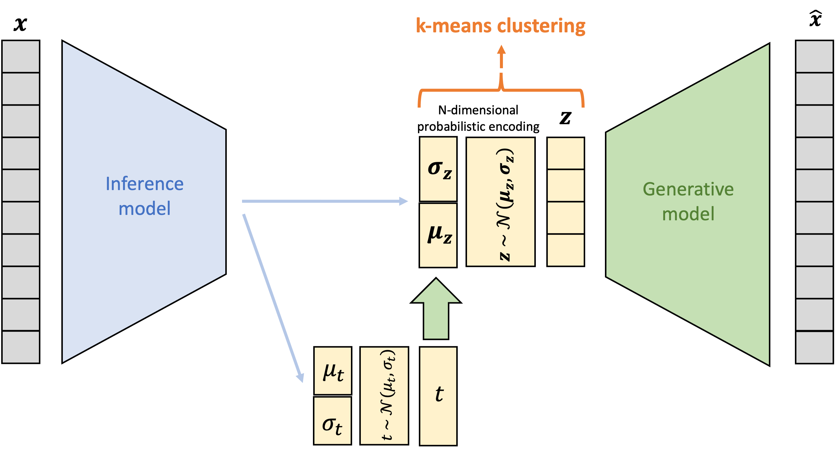
Figure 2: Schematic diagram of the R-VAE + k-means method which combines a VAE encoder with a prediction task, and subsequently clusters the resulting latent space using k-means to identify the weather regimes. Based on the architecture developed by Zhao et al. (2019a)

2.3.1 Variational inference

For a standard variational autoencoder, represented as a probabilistic graphical model in Figure 3a, with latent variables $z$, input data $x$ and parameters $\theta$, the normalization constant $p_{\theta}(\boldsymbol{x})=\int p_{\theta}(\boldsymbol{x},\boldsymbol{z})\text{d}z$ required to compute the model posterior $p_{\theta}(\boldsymbol{z}\mid\boldsymbol{x})$ is, in general, computationally intractable. To resolve this, the loss function of a variational autoencoder is derived using Bayesian variational inference (Murphy, 2023). Variational inference introduces a function $q_{\phi}$ from a selected distributional family with parameters $\phi$ to approximate the intractable posterior by minimizing the following Kullback-Leibler divergence between the true and approximated posterior:

$$\phi^{*} =\text{argmin}_{\phi}D_{KL}\left(q_{\phi}(\boldsymbol{z}\mid\boldsymbol{x}),p_{\theta}(\boldsymbol{z}\mid\boldsymbol{x})\right)$$

$$=\text{argmin}_{\phi}\mathbb{E}_{q_{\phi}(\boldsymbol{z})}[\log{q_{\phi}(\boldsymbol{z}\mid\boldsymbol{x})}-\log{p_{\theta}(\boldsymbol{z}\mid\boldsymbol{x})}-\log{p_{\theta}(\boldsymbol{z})}]+\log{p_{\theta}(\boldsymbol{x})}$$

$$=\text{argmin}_{\phi}\mathcal{L}(\theta,\phi\mid\boldsymbol{x})+\log{p_{\theta}(\boldsymbol{x})}.$$ (2)

The Evidence Lower Bound $\mathcal{L}(\theta,\phi\mid\boldsymbol{x})$, which is the part of the KL-divergence that depends on the parameters $\phi$, can then be minimized to provide a best variational estimate of our model, using, for example, the Expectation-Maximization Algorithm (Murphy, 2023). Kingma and Welling (2013) adapt variational inference to autoencoders using the Stochastic Gradient Variational Bayes (SGVB) estimator and introduce a reparameterization trick to generate samples from the probabilistic encoder $q_{\phi}(\boldsymbol{z}\mid\boldsymbol{x})$ while still being able to backpropagate information through the network.

2.3.2 Loss function derivation for the R-VAE method

The loss function for the extended variational autoencoder shown in Figure 3b, R-VAE, is derived similarly using Bayesian variational inference. Here, the inference model encodes not only the input space but also predicts a scalar target variable $t$. The latent space estimated by the encoder is then regularized by penalizing divergence from the latent space reconstructed from the predicted target variable. The resulting N-dimensional reduced space is clustered using k-means. Based on the assumptions encoded in the graphical model shown in Figure 3b, the joint probability distributions of the model can then be written as:

$$p_{\theta}(\boldsymbol{x},\boldsymbol{z},t)=p_{\theta}(\boldsymbol{x}\mid\boldsymbol{z})p_{\theta}(\boldsymbol{z}\mid t)p_{\theta}(t)\text{, and }q_{\phi}(\boldsymbol{z},t\mid\boldsymbol{x})=q_{\phi}(\boldsymbol{z}\mid\boldsymbol{x})q_{\phi}(t\mid\boldsymbol{x}).$$ (3)

Based on these assumptions, the following loss function is derived as the KL divergence of the two probability distributions, for the full derivation see appendix LABEL:appendixloss:

$$\mathcal{L}(\boldsymbol{x}) =-D_{KL}\left(q_{\phi}(\boldsymbol{z},t\mid\boldsymbol{x})\mid p_{\theta}(\boldsymbol{z},\boldsymbol{x},t)\right)$$ (4)

$$=\mathbb{E}_{q_{\phi}(\boldsymbol{z}\mid\boldsymbol{x})}\left[\log p_{\theta}(\boldsymbol{x}\mid\boldsymbol{z})\right]-\mathbb{E}_{q_{\phi}(t\mid\boldsymbol{x})}\left[D_{KL}(q_{\phi}(\boldsymbol{z}\mid\boldsymbol{x})\mid p_{\theta}(\boldsymbol{z}\mid t))\right]-D_{KL}\left(q_{\phi}(t\mid\boldsymbol{x})\mid p_{\theta}(t)\right).$$

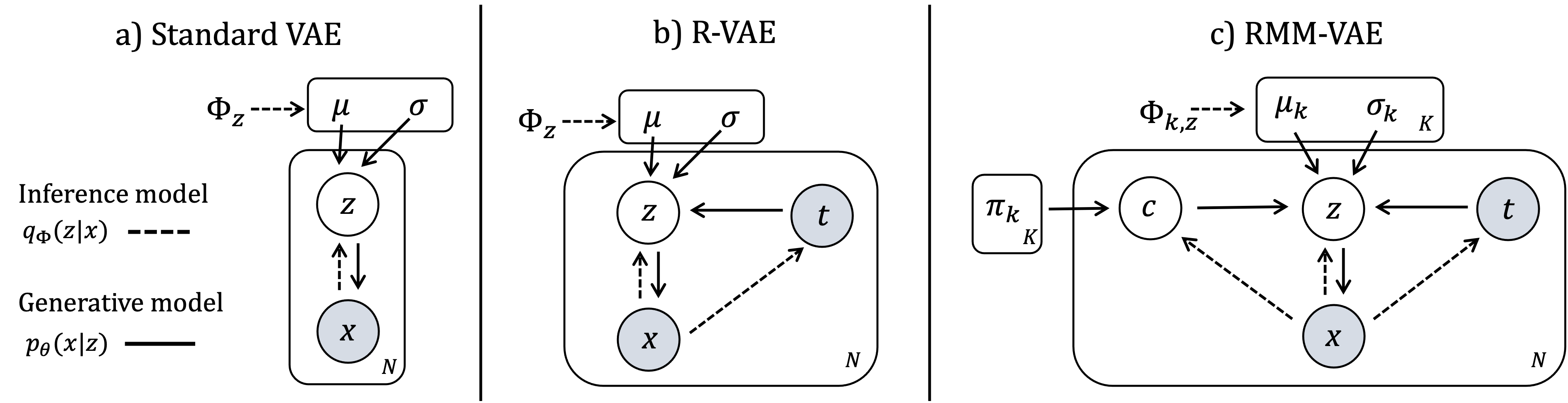
Figure 3: Different variational autoencoder models represented as probabilistic graphical models using plate notation. a) A standard VAE with input variable $\boldsymbol{x}$, latent variable $\boldsymbol{z}$, prior $\Phi_{z}$ and parameters $\theta$, b) the R-VAE method with an additional target variable $t$, and c) the RMM-VAE method with probabilistic cluster assignment $\boldsymbol{c}$ with prior $\Pi_{k}$. In all panels, dashed lines indicate the inference model and solid lines the generative model

The two components of the inference model, $q_{\phi}(\boldsymbol{z}\mid\boldsymbol{x})$ and $q_{\phi}(t\mid\boldsymbol{x})$, are parametrized as N-dimensional Gaussian distributions and estimated using non-linear functions with parameters $\phi$. Similarly, the probabilistic decoder is parametrized as a Gaussian and the mean modelled as a nonlinear function with parameters $\theta$. Under the assumption that the decoder captures the nonlinearity of the generative model, a linear model for $p_{\theta}(\boldsymbol{z}\mid t)\sim\mathcal{N}(\boldsymbol{a}t,\mathbb{I})$ is implemented, where $\boldsymbol{a}$ is a vector of unit norm. This constrains the number of parameters the model has to fit overall.

As in the standard VAE model, the first term represents the reconstruction loss of the dimensionality reduction, while the third term penalizes divergence of the predicted target variable $q_{\phi}(t\mid\boldsymbol{x})$ from the ground truth data $p(t)$. The second term holds the key to understanding this targeted approach to dimensionality reduction: there are two estimations of the latent space in the model, one based on a pure dimensionality reduction of the original data $q_{\phi}(\boldsymbol{z}\mid\boldsymbol{x})$, and one based on the predicted target variable $p_{\theta}(\boldsymbol{z}\mid t)$. The second term penalizes the divergence between those two terms which represent the two objectives of the model, weighted by the estimate of the target variable $q_{\phi}(t\mid\boldsymbol{x})$. Finally, k-means is applied to the dimensionality reduced space z which is an output of the non-linear encoder.

2.4 Regression - Mixture Model Variational Autoencoder (RMM-VAE)

While the R-VAE + k-means method directly includes a target variable in the identification of weather regimes, it implements the targeted dimensionality reduction, using a multi-dimensional Gaussian to regularize the latent space, and the clustering in two separate steps, which is somewhat duplicative.

Therefore, we propose a new approach, RMM-VAE, which fits a Gaussian mixture model, an established probabilistic clustering method (Murphy, 2022; Feldstein and Franzke, 2017), directly into the latent space instead of performing the clustering in a separate step, thereby estimating both targeted and probabilistic weather regimes in one coherent statistical model. More precisely, the multi-dimensional Gaussian chosen to regularize the latent space in the R-VAE method is replaced by $k$ individual Gaussians with mean $\boldsymbol{\mu_{k}}$ and standard deviation $\boldsymbol{\sigma_{k}}$. In addition, the probability $c_{ik}$ of the datapoint $x_{i}$ belonging to cluster $k$ is estimated. This builds on architectures combining variational autoencoders with mixture models presented, for example, by Ye and Bors (2020), Zhao et al. (2019b) and Jiang et al. (2017). An illustration of the model developed in this paper that incorporates a targeted dimensionality reduction with a mixture model fit is shown in Figure 4.

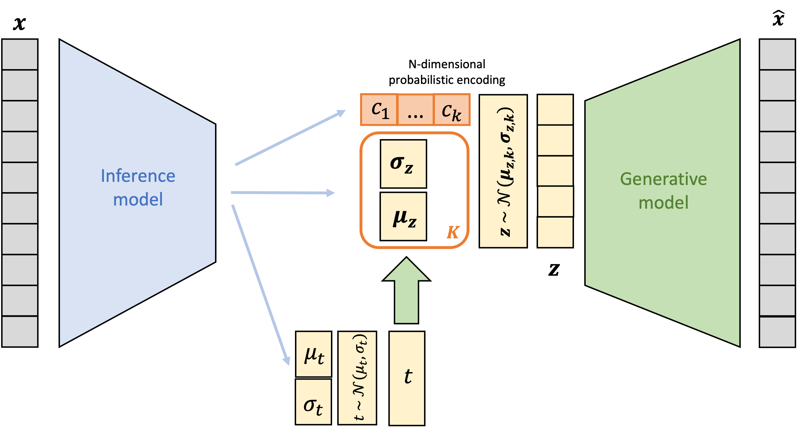
Figure 4: Schematic diagram of the proposed RMM-VAE approach, which combines a regression VAE (R-VAE) with probabilistic clustering using mixture models (MM) to identify the weather regimes

As for the R-VAE method, the conditional independence assumptions embedded in the corresponding graphical model shown in Figure 3c are used to re-write the joint probability distribution of the model and derive the loss function of the model:

$$\mathcal{L}(\boldsymbol{x}) =-D_{KL}(q_{\phi}(\boldsymbol{z},\boldsymbol{c},t\mid\boldsymbol{x})\mid p_{\theta}(\boldsymbol{x},\boldsymbol{z},t,\boldsymbol{c}))$$

$$=\sum_{k}q_{\phi}(\boldsymbol{c^{k}}\mid\boldsymbol{x})\bigg{[}\mathbb{E}_{q_{\phi}(\boldsymbol{z}\mid\boldsymbol{x})}[\log p_{\theta}(\boldsymbol{x}\mid\boldsymbol{z})]-\mathbb{E}_{q_{\phi}(t\mid\boldsymbol{x})}[D_{KL}(q_{\phi}(\boldsymbol{z}\mid\boldsymbol{x})\mid p(\boldsymbol{z}\mid t))]$$

$$-D_{KL}(q_{\phi}(t\mid\boldsymbol{x})\mid p(t))-D_{KL}(q_{\phi}(\boldsymbol{z}\mid\boldsymbol{x})\mid p_{\theta}(\boldsymbol{z}\mid\boldsymbol{c^{k}}))\bigg{]}-D_{KL}(q_{\phi}(\boldsymbol{c^{k}}\mid\boldsymbol{x})\mid p(\boldsymbol{c^{k}})).$$ (5)

The first three terms in brackets correspond to the terms of the R-VAE loss function for an individual mixture component: the reconstruction loss, the divergence of the estimated target variable $q_{\phi}(t\mid\boldsymbol{x})$ from the ground truth data, and the divergence between the latent spaces generated from the target variable $p(\boldsymbol{z}\mid t)$ and the latent space encoded from the input data $q_{\phi}(\boldsymbol{z}\mid\boldsymbol{x})$), all weighted by the cluster assignment $q_{\phi}(\boldsymbol{c^{k}}\mid\boldsymbol{x})$. The fourth term of the loss function minimizes the divergence between the cluster mean k and the latent space estimated from the input data, again weighted by the probability of cluster k occurring, $q_{\phi}(\boldsymbol{c^{k}}\mid\boldsymbol{x})$. The final term regularizes the cluster assignment $q_{\phi}(\boldsymbol{c^{k}}\mid\boldsymbol{x})$ to the previous cluster occurrence frequency $p(c^{k})$.

The components of the inference model $q_{\phi}(\boldsymbol{z}\mid\boldsymbol{x})$ and $q_{\phi}(t\mid\boldsymbol{x})$, and generative model $p_{\theta}(\boldsymbol{x}\mid\boldsymbol{z})$ and $p_{\theta}(\boldsymbol{z}\mid t)$, are parametrized as in the previous method. $p(c^{k})$ is a categorical distribution populated by the occurrence frequency of the different clusters updated at each step. This occurrence frequency is used as prior for the probabilistic cluster assignment of an individual day $q_{\phi}(\boldsymbol{c^{k}}\mid\boldsymbol{x})$. Individual mixture components $p(\boldsymbol{z}|\boldsymbol{c^{k}})$ are modelled as Gaussians with mean $\mu$ and the identity covariance matrix. The latter choice is made to constrain the number of parameters and avoid model overfitting. The same choices of layer number, epochs, and activation function as for the R-VAE method were adopted here.

3 Experiments

3.1 Data

We compute weather regimes over the Mediterranean region (lat: 25°N - 50°N; lon: 20°W - 45°E) in extended winter (Nov - Mar). The study focuses on the extended winter months as most of the observed annual as well as extreme precipitation and associated flood events over Morocco have occurred during this season (Loudyi et al., 2022). As input data, we use ERA5 reanalysis data from 1940 to 2022 (Hersbach et al., 2020) of geopotential height at 500hPa (z500) re-gridded to a resolution of 2.5°x2.5°. The data was standardized by subtracting the climatological daily mean and dividing the result by the standard deviation over the entire extended winter.

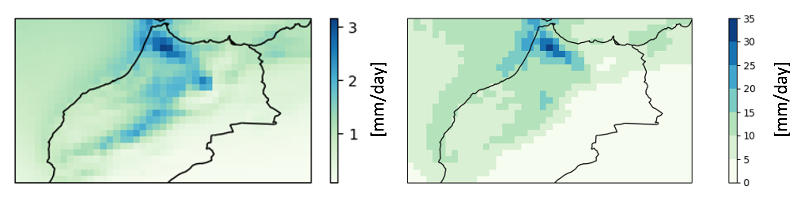
Figure 5: Extended winter precipitation (November - March) over the selected region over Morocco based on ERA5 reanalysis data from 1940-2022. Left-side: daily mean precipitation. Right-side: 95th percentile of daily precipitation

As the target variable, ERA5 reanalysis data of daily total precipitation in a region over Morocco (lat: 30°N — 36°N; lon: 11°W — 0°E, resolution: 0.5°x0.5°) over the same period was used. Figure 5 shows the annual mean and 95th-percentile precipitation over the selected region. Precipitation data was normalized by applying a Box-Cox transformation at each grid cell (Box and Cox, 1964). A three-day running average of daily total precipitation and a five-day running average of z500 were taken to reflect the duration of extreme precipitation events and associated weather systems during the observational period (Dayan et al., 2015; Loudyi et al., 2022; Ullmann et al., 2014).

3.2 Parameter choices and implementation

The encoders of both VAE methods are implemented using three dense layers of decreasing dimensionality of 128, 64 and 28 respectively. A batch size of 64 and the ReLU activation function are chosen. For 100 epochs, the model is first trained on a training set comprised of two-thirds of the data and tested on the remaining third, and subsequently fitted again using a random weights initialization on the entire dataset. For the implementation of the neural network architectures, the Python package keras (Chollet et al., 2015) was used. For a number of the evaluation metrics as well as the implementation of the two linear methods, the Python package scikit-learn (Pedregosa et al., 2011) was employed.

Table 1 provides an overview of the compared methods along with relevant hyperparameters. A 10-dimensional latent space was implemented for all the methods, and cluster numbers between 4 and 10 were investigated based on the understanding that the correct number of clusters will depend on the use case (Feldstein and Franzke, 2017) and cannot be determined in a general sense in all regions. The sensitivity of the results to both these choices was investigated, with the sensitivity of the clusters to sub-sampling for different choices of k shown in Appendix LABEL:appendixA. Based on these results, k=5 was identified as a reasonable choice of cluster number to visualise in the results section where required.

For both VAE methods, the inclusion of a hyperparameter $\beta$ based on Higgins et al. (2017) is investigated. The hyperparameter is multiplied with the respective first terms in equations 4 and 2.4 which represent the reconstruction loss, thereby changing the weight of the reconstruction objective in the loss function. Two values of $\beta$ are explored for each of the two methods, whereby v1 ($\beta=1$) corresponds to the original loss function without the inclusion of an additional hyperparameter, and v2 ($\beta<1$) decreases the importance of the reconstruction loss term in the loss function. Selected values for $\beta$ are shown in table 1.

Table 1: Overview of methods for the identification of weather regimes and associated parameter choices.

Abbreviation	Method	$\beta$	Precipitation data
PCA	PCA + k-means	-	None
CCA	CCA + k-means	-	$\boldsymbol{t}$ - full daily precipitation field at 0.25° resolution
R-VAE v1	R-VAE + k-means	1	$t$ - spatially averaged daily precipitation (scalar)
R-VAE v2	R-VAE + k-means	0.1	" - "
RMM-VAE v1	RMM-VAE	1	" - "
RMM-VAE v2	RMM-VAE	0.5	" - "

4 Results

The four methods PCA + k-means, CCA + k-means, R-VAE + k-means and RMM-VAE, are compared along different evaluation metrics chosen to cover three objectives of targeted clustering: representation of the complete phase space of atmospheric circulation, predictive skill, and cluster robustness. The identified weather regimes and associated precipitation patterns over Morocco are presented in the final section of the analysis.

4.1 Investigating the targeted dimensionality reduced space

The dimensionality-reduced spaces of different methods are investigated by projecting the 10-dimensional, already dimensionality-reduced space onto two dimensions using t-distributed stochastic nearest neighbour embedding (t-SNE) (Maaten and Hinton, 2008), a method commonly applied in the machine learning community for the visualisation of high-dimension datasets. In the case of PCA, for example, the first 10 principal components that span the latent space are projected onto two dimensions, visualised below. For the VAE methods, the 10-dimensional probabilistic latent space $p_{\theta}(\boldsymbol{z}\mid\boldsymbol{x})$ is projected onto two dimensions. The resulting visualisation, shown in Figure 6, provides an intuition for how the target variable is distributed in the dimensionality-reduced space, and how different clustering methods capture this distribution.

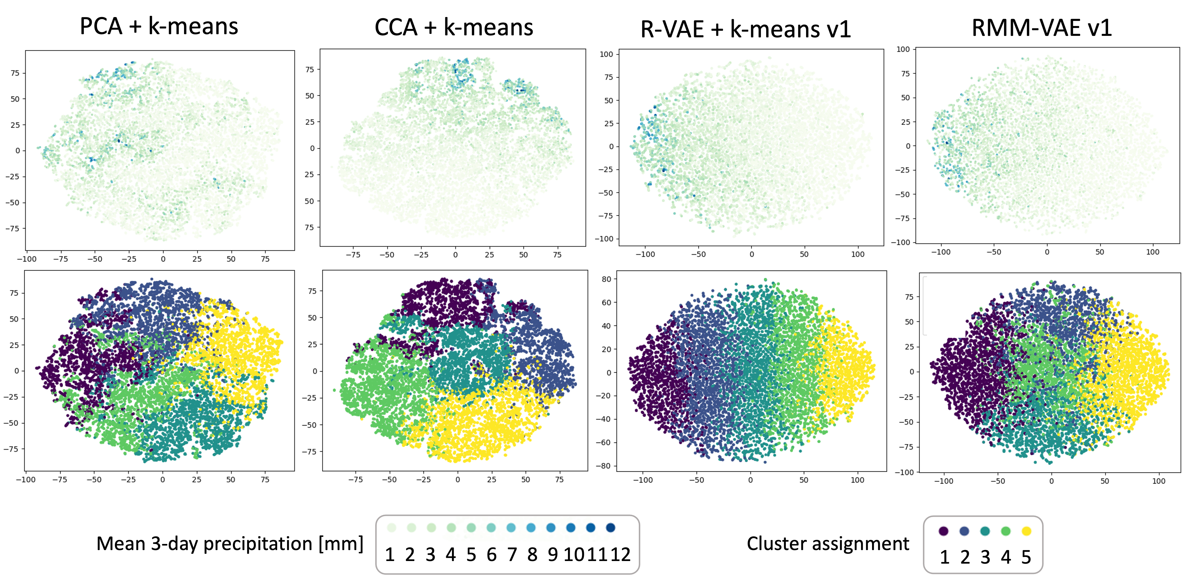
Figure 6: Visualisation of the 10-dimensional latent spaces in two dimensions using t-distributed stochastic nearest-neighbour embedding (t-SNE). Different values of perplexity were tested and perplexity=10 was chosen as it shows representative results. Embedded data points are coloured according to the value of the target variable, total mean precipitation (top row), and according to the cluster they are subsequently assigned to (bottom row)

Both targeted VAE methods, R-VAE and RMM-VAE, disentangle the dimension of the high-dimensional z500 input dataset associated with the scalar target variable $t$ (dark dots in Figure 6, top row), which is in line with the findings presented by Zhao et al. (2019a) for the R-VAE method. The PCA latent space, on the other hand, shows little organisation with respect to the target variable, as expected, since the target variable is not part of the dimensionality reduction. In contrast, the CCA latent space appears to have more structure compared to PCA.

However, the R-VAE + k-means and RMM-VAE methods structure the clusters differently in their respective latent space (Figure 6, bottom row): the R-VAE + k-means method, which carries out dimensionality reduction and clustering in two separate steps, orders clusters in bands along a dimension associated with the target variable. In contrast, the RMM-VAE method, which fits probabilistic clusters while simultaneously disentangling the dimension associated with the target variable, organises the clusters in a way that appears more consistent with the target of minimizing the distance between points in one cluster, which is also the case for PCA + k-means and CCA + k-means. A possible explanation for this is that the R-VAE method stretches the distance between points along the dimension associated with the target variable in the reduced dimensionality space, so that the distance-based k-means algorithm identifies clusters that appear as bands along the target dimension. This effect is not observed in the other methods as neither PCA nor CCA target their latent space in this specific way, while the RMM-VAE method fits the clusters while simultaneously targeting the latent space, and therefore may not stretch the distance between points along the target dimension in the same way. While the bands identified by the R-VAE + k-means method possibly aid the predictive skill of the clusters, they also impact cluster persistence and robustness, which will be explored further below.

4.2 Comparing reconstruction loss across methods

The performance of the dimensionality reduction component of the method is assessed by computing the mean squared error (MSE) between input data and data reconstructed from the latent space. In the case of PCA, for example, the input data point is compared to that same data point reconstructed using the first 10 principal components. In the case of the VAE methods, the input data point is compared to that same data point after passing it through the encoder and decoder of the model. The lower this value, the more information about the input space is captured by the dimensionality reduction method (PCA, CCA, R-VAE or RMM-VAE respectively). Figure 7 shows the distribution of this error across all data points.

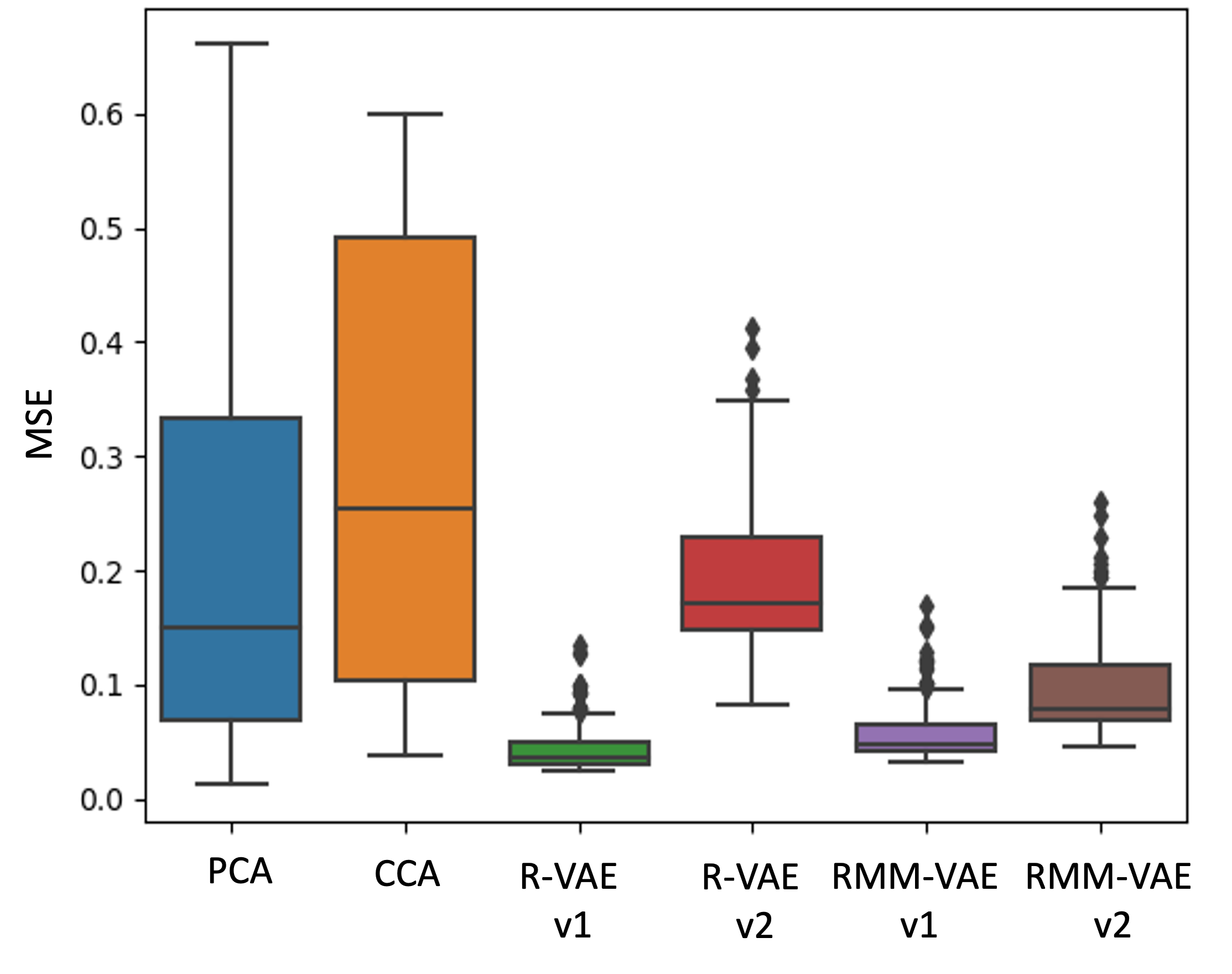
Figure 7: Distribution of mean squared error (MSE) between original input data and data reconstructed from the dimensionality-reduced space over all data points, for the different methods

Both VAE v1 methods (with $\beta$=1) have a lower and less widely distributed RMSE compared to both PCA and CCA. This means that despite targeting their respective latent spaces to an impact variable, the VAE v1 methods still capture more information about the input space than the two linear methods.

When increasing the importance of the prediction objectives in the VAE v2 models (with $\beta$<1), both R-VAE v2 and RMM-VAE v2 still outperform PCA and CCA but perform worse than their respective v1 counterparts. RMM-VAE v2 ($\beta$=0.5) performs slightly better than R-VAE v2 ($\beta$=0.1) which is consistent with the different values for $\beta$ chosen to ensure convergence of the model.

Investigating the reconstruction of an individual data point, shown in Figure 8, we find that both v2 methods and CCA focus the dimensionality reduction on the Western Mediterranean region surrounding Morocco. This result shows that a trade-off between targeting the dimensionality reduction and reconstructing the full phase space exists, although the two VAE v1 methods that are based on targeted dimensionality reduction nevertheless perform best in reconstructing the input space.

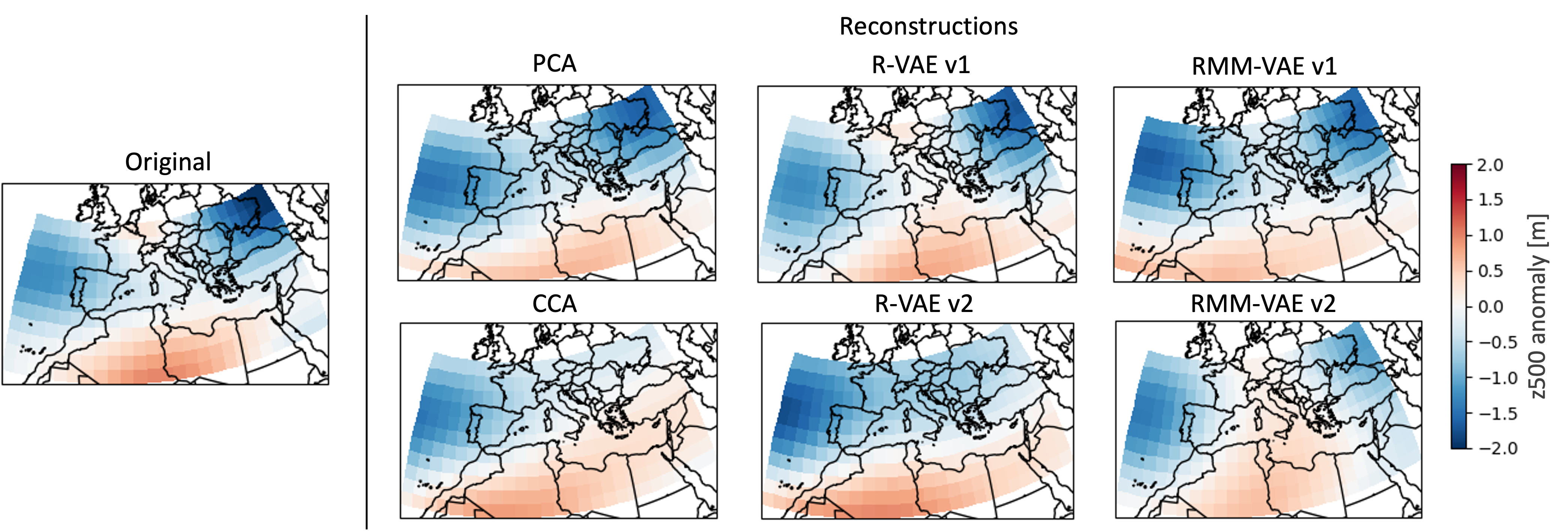
Figure 8: Gridded and normalized z500 anomalies, as detailed in Section 3, on an example day 1940-01-04, showing the original data on the left and the reconstructions using different methods on the right

4.3 Evaluating the predictive skill of weather regimes

To evaluate the informativeness of the weather regimes with respect to the target variable, and, in particular, their utility for extended-range forecasting, we analyse the Ranked Probability Score (RPS) which is defined as

$$RPS=\frac{1}{N}\sum_{n=1}^{N}\sum_{j=1}^{m}(\delta_{i_{n}j}-p_{j})^{2}=-\frac{1}{N}\sum_{n=1}^{N}(1-2p_{i_{n}}+\sum_{j=1}^{m}p_{j}^{2}),$$ (6)

where $m$ is the number of forecast categories and $N$ the number of timesteps. $\delta_{i_{n}j}$ is the Kronecker delta which equals 1 if the observation $i$ at timestep $n$ corresponds to category $j$, and 0 otherwise. The RPS is a strictly proper scoring rule to measure the accuracy of a probabilistic prediction of mutually exclusive discrete outcomes (Gneiting and Raftery, 2007) and is widely used in forecast evaluation. The corresponding skill score (RPSS) is calculated with respect to a reference forecast, chosen here to be the climatology over the entire period, defined as

$$RPSS=1-\frac{RPS_{\text{forecast}}}{RPS_{\text{climatology}}}.$$ (7)

A RPSS of 1 indicates a perfect forecast while low values indicate little, or no skill compared to the reference forecast. Here, a forecast of the target variable is constructed given the occurrence of a weather regime and the conditional probability of the target variable given that weather regime: each discrete target is forecast with a probability corresponding to the probability of the weather regime at this given day, multiplied by the climatological conditional probability of the target given the weather regime.

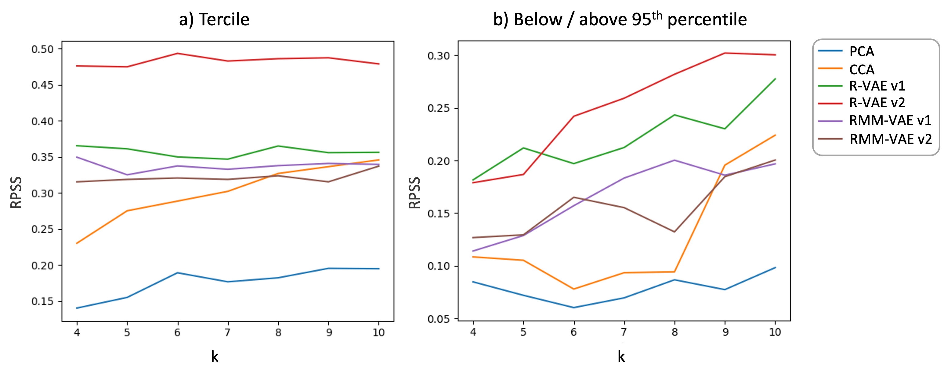
Figure 9: Ranked Probability Skill Score for forecast of mean precipitation over Morocco given weather regimes for different numbers of weather regimes k. a) Skill score for the forecast of the tercile of the precipitation distribution, and b) Skill score for a binary forecast above or below the 95th percentile. For probabilistic clustering, the skill score is computed using the most likely cluster at the given data point

Using the RPSS, the predictive skill of the different weather regimes is evaluated in terms of predicting precipitation terciles (Figure 9a), as well as extreme precipitation, defined here as the 95th percentile of total precipitation over the area (Figure 9b). The predictive skill is overall higher for terciles compared to the 95th percentile threshold, which is to be expected. Across both prediction targets, all targeted methods outperform PCA + k-means (blue line), highlighting the potential of improving the predictive skill of standard weather regime definitions. R-VAE + k-means (green and red lines) performs best, followed by RMM-VAE (purple and brown lines) up to k=8. The better performance of R-VAE can be attributed to RMM-VAE having more objectives to achieve simultaneously compared to R-VAE, as it aims to identify optimal clusters while disentangling the latent space with respect to the target variable at the same time. For both VAE methods, increasing the importance of the prediction objective in the loss function (v2) further boosts the predictive skill. This demonstrates the trade-off between the prediction and dimensionality reduction objectives but again shows that the VAE v1 methods are effective in improving the predictive skill of clusters while capturing information about the input space more effectively than the baseline linear methods.

Increasing the number of clusters does not improve the skill except for CCA + k-means. For the two VAE methods, this result is likely because the targeted dimensionality reduction already groups data points with similar precipitation amounts in the reduced space. Unlike the other methods, CCA takes the full precipitation field as input. The ability to extract spatial information about the precipitation field might enable the predictive skill to increase with cluster number, as will be discussed further below.

4.4 Cluster persistence and separability

Persistence, separability, and statistical robustness are required for the weather regimes to be meaningful and to provide extended-range predictive skill. Figure 10a shows the distribution of mean persistence for each of the k=5 clusters and Figure 10b the silhouette score which is a measure of cluster separability for a range of cluster numbers (Rousseeuw, 1987). The higher the silhouette score, the better the clusters are separated from one another, while a silhouette score close to zero indicates that the separation between different clusters is not statistically significant. Furthermore, the sensitivity of cluster centres to subsampling is investigated with results shown in Appendix LABEL:appendixA.

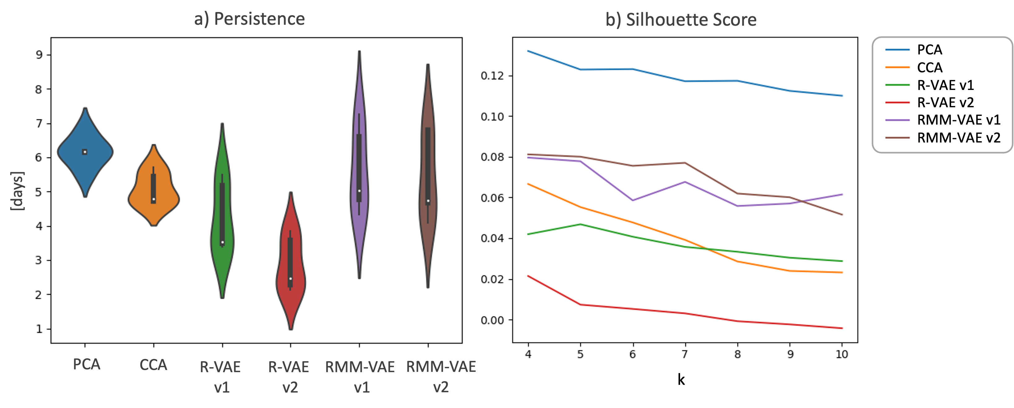
Figure 10: Cluster persistence and separability. a) Cluster persistence in days for $k=5$ clusters. Violin plots show the kernel density estimation of the distribution, the distribution median (white point) as well as the interquartile range (black box). The ranking of different methods in terms of persistence remains the same for different choices of $k$. b) Silhouette score which is a measure of cluster separation for a range of cluster numbers k (Rousseeuw, 1987). The silhouette score is defined as the mean silhouette coefficient (b-a)/max(a,b), where a is the average intra-cluster distance and b is the average inter-cluster distance i.e. the average distance between all clusters

Mean persistence across clusters is highest for PCA, followed by RMM-VAE. However, the spread of the distribution is lower for PCA and CCA compared to the two VAE methods, in particular RMM-VAE. This result indicates that while all five PCA + k-means clusters have around the same average persistence, there are some clusters with a longer and some with a shorter average persistence identified by the VAE methods. These results are qualitatively similar for other choices of k (not shown). Sample time series of the cluster assignments in different methods are shown in appendix LABEL:appendixB.

All targeted clusters perform worse in terms of cluster separability (Fig. 10b) compared to the baseline method PCA. RMM-VAE outperforms the other targeted methods while R-VAE performs the worst overall. This supports the initial exploration presented in Section 4.1, where the RMM-VAE clusters were found to be more coherently organized in the latent space compared to the R-VAE clusters. Overall, these results indicate that RMM-VAE identifies more coherent and robust clusters compared to the other targeted methods. This highlights the benefit of performing the probabilistic clustering in one coherent statistical model, predicting the target variable and dimensionality reducing the input space in a single step, as opposed to separating the two steps, as in the R-VAE + k-means method.

4.5 Cluster characteristics

In the final step of the analysis, the cluster centres identified by different methods are investigated, along with the associated change in the conditional probability of extreme precipitation, shown in Figure 11. This provides insight into the processes that the targeted weather regimes capture to enhance their predictive skill, as well as the differences between the targeted clustering methods investigated.

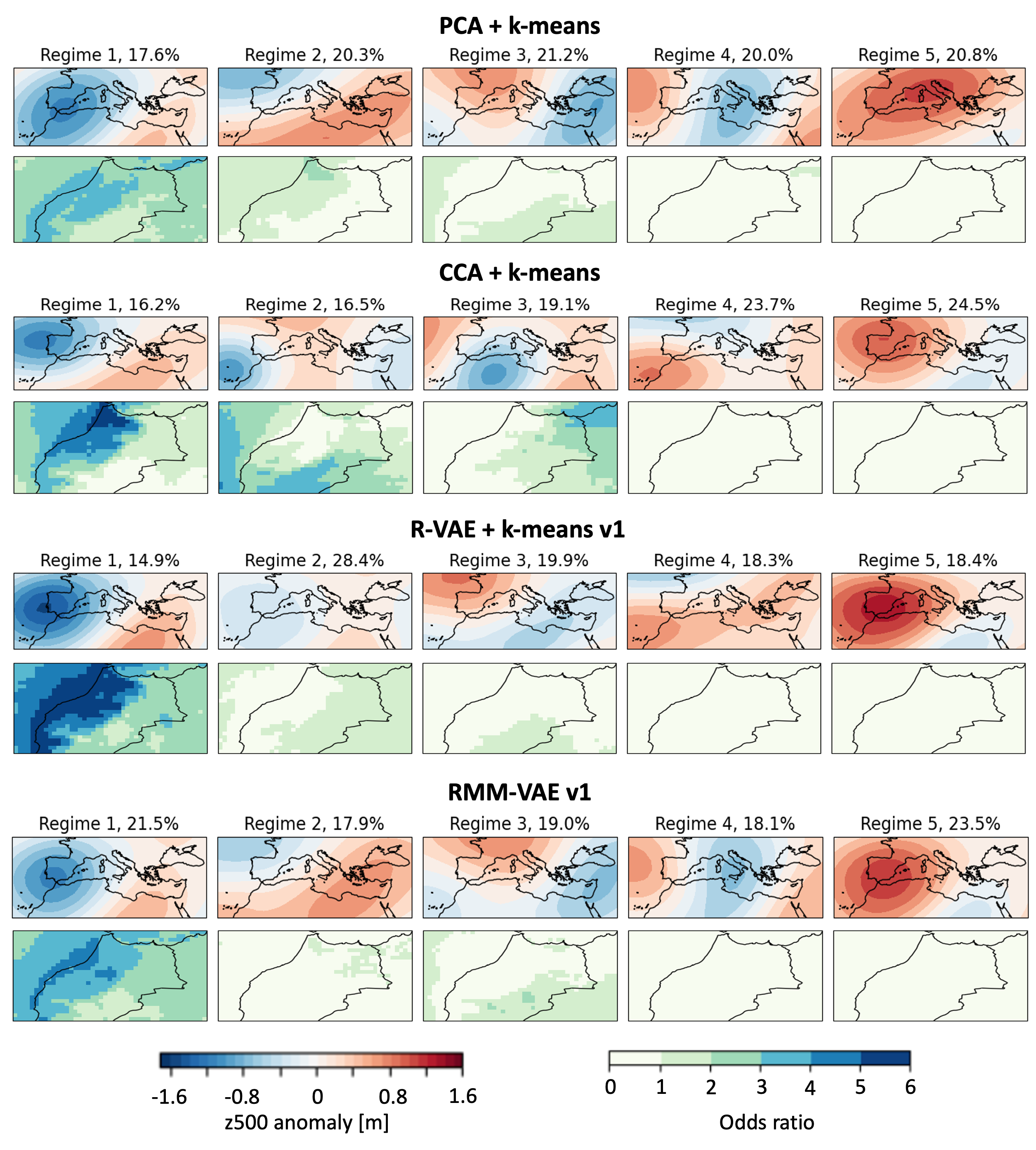
Figure 11: Cluster centres of z500 geopotential height calculated using different methods with the cluster number specified as $k=5$ and z500 standardized as described in the section 3.1. For the probabilistic cluster method RMM-VAE, the means of the fitted mixture components are shown. For each method, the corresponding odds ratio of extreme precipitation is shown below the cluster centre: for each grid cell, this corresponds to the ratio of the conditional probability of the climatological 95th percentile of precipitation at the grid cell conditional on that weather regime, divided by the unconditional probability of 95th percentile of precipitation (i.e. 0.05). The cluster centres are ordered in decreasing order of mean precipitation during the days assigned to this cluster by the method

The cluster centres identified by PCA + k-means correspond to the weather regimes identified over the Mediterranean region in other publications using this method such as Giuntoli et al. (2022) and Mastrantonas et al. (2022). While the number of regimes investigated varies, both publications identify the meridional patterns observed in regimes 3 and 4, a high geopotential height anomaly (regime 5 - termed Mediterranean high in Mastrantonas et al. (2022)), and the western low anomalies seen in regimes 1 and 2, (termed Iberian and Biscay Low in Mastrantonas et al. (2022)). Regime 1, associated with a geopotential height low over the west of Europe increases the probability of extreme precipitation by a factor of 3-4, which is consistent with the results found by Mastrantonas et al. (2020), while the other regimes show no or marginal increases in the probability of extreme precipitation. Overall, the regimes identified by PCA + k-means have roughly similar frequencies of occurrence.

CCA + k-means identifies multiple regimes associated with an increase in the conditional probability of extreme precipitation by a factor of three or more in different regions of Morocco (regimes 1-3). The spatial pattern of extreme precipitation appears to be modulated by the location of the geopotential height low around Morocco. In contrast, high geopotential height anomalies dominate over the western Mediterranean in the two regimes associated with a lower-than-average probability of extreme precipitation. The regimes associated with extreme precipitation (1-3) have a slightly lower frequency of occurrence than the other two (4-5). Recalling that CCA performed worst of all methods in reconstructing the input space, particularly over the Eastern Mediterranean, consequently, the main anomalies that define the CCA + k-means cluster centres are located in the Western Mediterranean region.

In contrast to the different spatial patterns of extreme precipitation associated with three weather regimes identified using CCA + k-means, the R-VAE + k-means method identifies a single regime associated with a 5-6 times increase in the probability of extreme precipitation. Furthermore, we find that the cluster centre of regime 2, which occurs on almost 30% of days, shows very little mean z500 anomaly, meaning it is quite close to a climatologically average day in extended winter. This supports the results presented in the previous sections that show that while R-VAE + k-means succeeds at targeting the dimensionality reduction (see regime 1), it falls short in terms of identifying structure in the atmospheric phase space compared to the other methods.

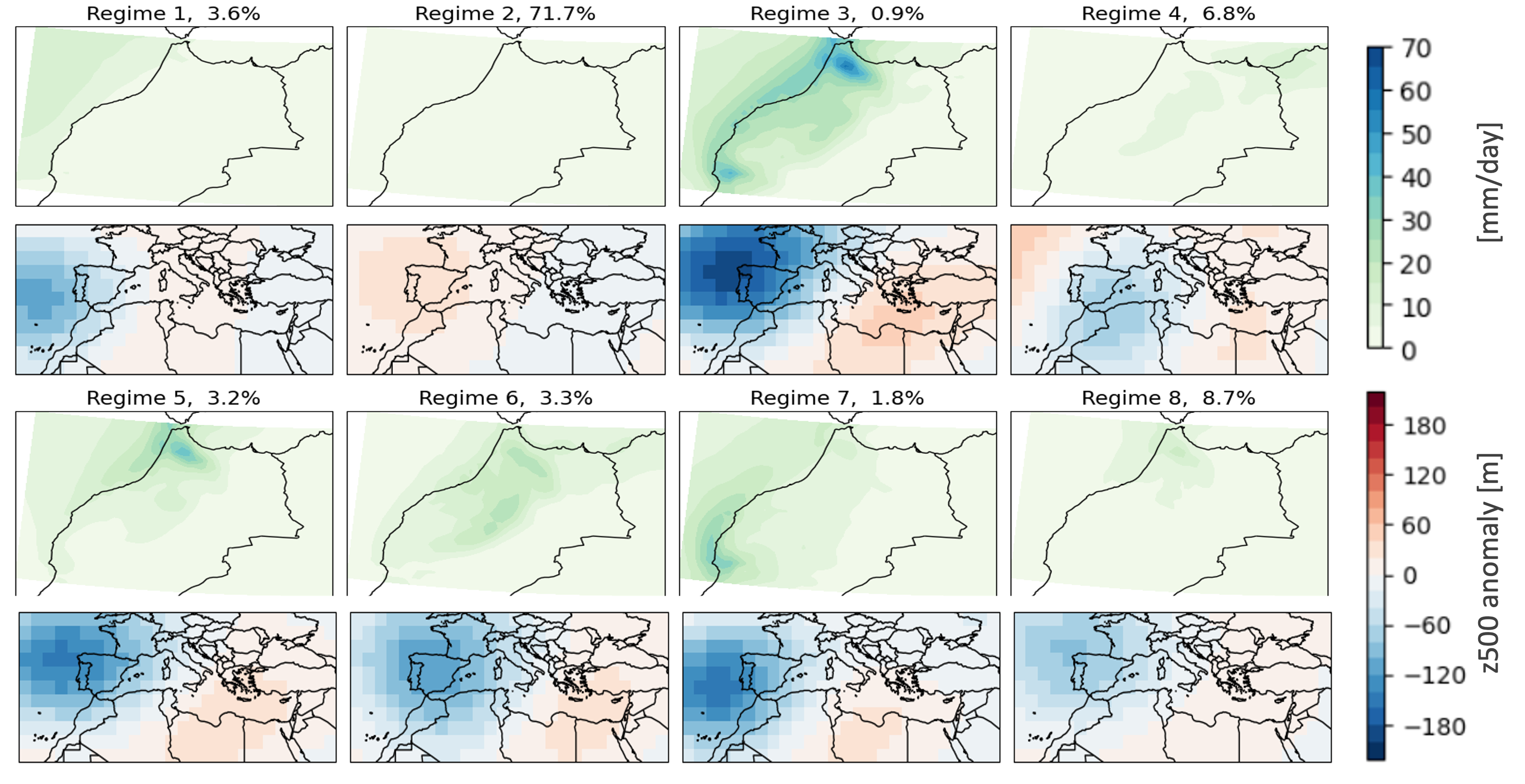
Figure 12: Precipitation clusters computed on precipitation reanalysis data without pre-processing using the k-means clustering algorithm (top rows) and mean z500 anomalies during precipitation clusters (bottom rows)

The RMM-VAE method, in terms of cluster centres, appears to strike a balance between the baseline method PCA + k-means, and the purely targeted method R-VAE + k-means. On the one hand, the method identifies a single regime associated with an increased probability of extreme precipitation, similar to R-VAE + k-means, reflecting the common organisation of the dimensionality-reduced input space (see figure 6). On the other hand, the resulting cluster centres are visually more similar to the PCA + k-means cluster centres, reflecting the fact that the RMM-VAE method targets the dimensionality-reduced space subject to concurrent clustering, hence balancing the two objectives.

To further investigate the geopotential height anomalies associated with different patterns of extreme precipitation, precipitation is clustered directly using k-means clustering and the associated mean anomalies in geopotential height are calculated, shown in figure 12. As discussed in section 1, clustering the impact variable directly compromises regime persistence and leads to an incomplete representation of the large-scale dynamics, and is therefore shown for illustration purposes only.

In agreement with the odds ratios associated with cluster centres shown in Figure 11, the location and intensity of the precipitation events appear to be modulated by the location and intensity of a geopotential height low off the coast of Spain. This finding is consistent with the literature on extreme precipitation events in the Western Mediterranean which highlights dynamically driven moisture flux from the Atlantic as a key driver (Dayan et al., 2015). Toreti et al. (2010) show that geopotential height anomalies associated with extreme precipitation over the Western Mediterranean, similar to those found in Figure 12, are associated with an alignment of the subtropical jet with the African coastline and anomalous southwesterly surface to mid-tropospheric flow which leads to large-scale ascending motions and instability over the Western Mediterranean region.

The two VAE methods cluster the different patterns of z500 anomalies identified in Figure 12 in one single weather regime, while CCA + k-means disaggregates some of the different spatial patterns of extreme precipitation into different weather regimes. This finding is consistent with the way the different methods incorporate the target variable: while CCA makes use of the entire precipitation field as input data and can hence extract more information about its spatial structure, the VAE methods only receive a single scalar target variable, total precipitation, as input.

5 Discussion and Conclusion

In this paper, we present a new machine learning method, RMM-VAE (Regression Mixture Model Variational AutoEncoder), for identifying weather regimes with respect to a scalar target variable. The novelty of the method lies in integrating the different objectives of targeted regimes, robust clustering and prediction of a target variable, in a coherent statistical model by combining non-linear and targeted dimensionality reduction with probabilistic clustering using mixture models based on a variational autoencoder architecture.

The RMM-VAE method is applied to identify weather regimes in 500 hPa geopotential height (z500) anomalies over the Mediterranean region targeted to precipitation over Morocco. Results are compared to three alternative approaches: principal component analysis (PCA) combined with k-means clustering as the currently established standard practice for identifying weather regimes (Bloomfield et al., 2020; Giuntoli et al., 2022), canonical correlation analysis (CCA) combined with k-means as an established statistical method to relate two high-dimensional input spaces (implemented, for example, by Vrac and Yiou (2010)), and R-VAE (regression variational autoencoder) combined with k-means clustering which extends a machine learning architecture presented by Zhao et al. (2019a). We evaluated the performance of all four methods with respect to the predictive skill of the weather regimes, the ability of the dimensionality reduction to capture information about the high-dimensional input space, and the robustness and persistence of the identified clusters.

Overall, the new RMM-VAE method performs well across all different objectives. It outperforms both linear methods (PCA + k-means and CCA + k-means) in terms of reconstructing the input space (Figure 7) and predicting the target variable up to a certain cluster number (Figure 9). While a more efficient reconstruction of the input space is expected from a generic VAE architecture due to the higher degrees of freedom when fitting the encoding function (Murphy, 2023), this result is non-obvious and relevant here, given that the presented RMM-VAE method additionally has the two other objectives of disentangling a scalar target variable and fitting probabilistic clusters. Compared to the other machine learning method (R-VAE + k-means), the RMM-VAE method loses in predictive skill. However, it identifies more persistent and separable clusters (Figure 10) compared to both targeted clustering methods, CCA + k-means and R-VAE + k-means. This is particularly relevant for climate applications such as extended-range forecasting where there is an explicit interest in the persistence and transition probabilities between clusters. The cluster centres shown in Figure 11 visually demonstrate the balancing act performed by the RMM-VAE method, and the identified weather regimes associated with extreme precipitation are in line with existing literature on the dynamical conditions driving extreme precipitation in the Western Mediterranean (Dayan et al., 2015).

Our analysis highlights multiple trade-offs when identifying targeted weather regimes. All targeted methods lose in terms of persistence and separability against the non-targeted baseline method PCA + k-means, although the RMM-VAE method still performs better than the other methods. Furthermore, a trade-off between reconstruction loss and predictive skill of the clusters is identified for the VAE architectures and made explicit by introducing a hyperparameter $\beta$ into the VAE models that allows to change the weight of the reconstruction term in the VAE loss functions. Improving the predictive skill of the target variable in the v2 versions ($\beta<1$) comes at the cost of reconstructing the full phase space in this model.

Making these trade-offs explicit highlights that the most appropriate method to navigate the different objectives of targeted clustering will depend on the use case at hand. For example, if there is research interest in the weather regimes themselves and their teleconnections with low-frequency climate patterns, robust and persistent clusters might be preferable. However, if the research interest is primarily in a statistical model that relates large-scale dynamics to local-scale impact, identifying persistent clusters of atmospheric dynamics might not be important.

Our novel RMM-VAE method explicitly incorporates these different objectives in a coherent probabilistic model rather than implicitly addressing them through the choice of cluster number (Gadouali et al., 2020) or pre-filtering (Rouges et al., 2023). While the RMM-VAE method comes at the cost of rendering the approach more complicated and moving away from the explicit calculation performed in both PCA and CCA methods, it improves the performance of the targeted clustering along multiple objectives, allows incorporation of co-variates and priors in an explicit probabilistic model, and makes the inherent trade-offs when identifying targeted weather regimes explicit.

However, although both VAE methods, R-VAE + k-means and RMM-VAE, improve the predictive skill of clusters with regard to the target variable compared to both CCA and PCA for lower cluster numbers ($k<9$), CCA shows a better performance for higher cluster numbers albeit at the cost of a worse reconstruction and cluster persistence and separability. This is due to CCA using the entire high-dimensional space of the target variable to identify targeted subspaces and hence being able to distinguish different spatial patterns of extreme precipitation in different weather regimes, as can be seen in Figure 11. In contrast, RMM-VAE only considers a scalar target variable, which represents a limitation of our current architecture. In future work, the current modelling framework could be expanded to develop a joint clustering of two high-dimensional variables, building on prior work conducted by Chalupka et al. (2016) and Vrac and Yiou (2010).

While the impact variable explored here is 3-day precipitation over Morocco, in principle any impact variable, such as renewable energy supply and number of people impacted by an extreme event, that has a justifiable link to the large-scale meteorological variables, could be used. Future work could apply the method to other regions and target variables, in particular, more realistic and decision-relevant impact variables to explore its robustness and usefulness in practice. Furthermore, other limitations of existing methods such as their physical meaningfulness are not explicitly addressed in our method. However, additional meteorological variables such as moisture fluxes or the location of storm tracks conditional on the identified regimes can be analysed to investigate the physical basis underlying the identified targeted regimes. Finally, a number of a priori choices that are common to all clustering methods such as the region, pre-processing steps, the method of computing the anomalies and the low-frequency filter applied to the geopotential height data remain. Sensitivities to these choices are explored in Appendix LABEL:appendixA and should, where possible, be explicitly included in the method rather than seen as opaque a priori choices.

The machine learning method presented in this paper contributes to an existing pool of methods to statistically relate large-scale atmospheric dynamics to regional extremes in local-scale impact variables, which has a number of relevant applications such as dynamical adjustment and extreme event attribution, downscaling and forecast post-processing. In addition to introducing a new method, this paper also highlights the commonalities, benefits and drawbacks of novel machine learning methods compared to more established statistical methods, hopefully contributing to the further development of suitable machine learning methods to this application field.

Acknowledgments

The authors thank Jakob Wessel for useful discussions and feedback. ERA5 reanalysis data (Hersbach et al., 2020) was downloaded from the Copernicus Climate Change Service (C3S) (2023). The results contain modified Copernicus Climate Change Service information 2020. Neither the European Commission nor ECMWF is responsible for any use that may be made of the Copernicus information or data it contains.

Funding Statement

TGS and MK were funded by the European Commission Horizon 2020 project XAIDA (Extreme Events: Artificial Intelligence for Detection and Attribution), Grant Agreement No. 101003469. FRS is funded by the Advancing the Frontiers of Earth System Prediction (AFESP) Doctoral Training Programme.

Competing Interests

The authors declare no competing interests exist.

Data Availability Statement

The data used in this study is available on Zenodo https://zenodo.org/records/10101006. The scripts necessary to reproduce the results in this study can be found on GitHub: https://github.com/fiona511/RMM-VAE.

Ethical Standards

The research meets all ethical guidelines, including adherence to the legal requirements of the study country.

References

- Lemos et al. [2012] Maria Carmen Lemos, Christine J. Kirchhoff, and Vijay Ramprasad. Narrowing the climate information usability gap. Nature Climate Change, 2(11):789–794, November 2012. ISSN 1758-6798. doi:10.1038/nclimate1614. URL https://www.nature.com/articles/nclimate1614. Number: 11 Publisher: Nature Publishing Group.
- Coughlan de Perez et al. [2022] Erin Coughlan de Perez, Laura Harrison, Kristoffer Berse, Evan Easton-Calabria, Joalane Marunye, Makoala Marake, Sonia Binte Murshed, Shampa, and Erlich-Honest Zauisomue. Adapting to climate change through anticipatory action: The potential use of weather-based early warnings. Weather and Climate Extremes, 38:100508, December 2022. ISSN 2212-0947. doi:10.1016/j.wace.2022.100508. URL https://www.sciencedirect.com/science/article/pii/S2212094722000871.
- Ghil and Robertson [2002] Michael Ghil and Andrew W. Robertson. “Waves” vs. “particles” in the atmosphere’s phase space: A pathway to long-range forecasting? Proceedings of the National Academy of Sciences, 99(suppl_1):2493–2500, February 2002. ISSN 0027-8424, 1091-6490. doi:10.1073/pnas.012580899. URL https://pnas.org/doi/full/10.1073/pnas.012580899.
- Hannachi et al. [2017] Abdel. Hannachi, David M. Straus, Christian L. E. Franzke, Susanna Corti, and Tim Woollings. Low-frequency nonlinearity and regime behavior in the Northern Hemisphere extratropical atmosphere. Reviews of Geophysics, 55(1):199–234, 2017. ISSN 1944-9208. doi:10.1002/2015RG000509. URL https://onlinelibrary.wiley.com/doi/abs/10.1002/2015RG000509. _eprint: https://onlinelibrary.wiley.com/doi/pdf/10.1002/2015RG000509.
- Cassou [2008] Christophe Cassou. Intraseasonal interaction between the Madden–Julian Oscillation and the North Atlantic Oscillation. Nature, 455(7212):523–527, September 2008. ISSN 1476-4687. doi:10.1038/nature07286. URL https://www.nature.com/articles/nature07286. Number: 7212 Publisher: Nature Publishing Group.
- Gonzalez et al. [2022] Paula L. M. Gonzalez, Emma Howard, Samantha Ferrett, Thomas H. A. Frame, Oscar Martínez-Alvarado, John Methven, and Steven J. Woolnough. Weather patterns in Southeast Asia: Enhancing high-impact weather subseasonal forecast skill. Quarterly Journal of the Royal Meteorological Society, 2022. ISSN 1477-870X. doi:10.1002/qj.4378. URL https://onlinelibrary.wiley.com/doi/abs/10.1002/qj.4378. _eprint: https://onlinelibrary.wiley.com/doi/pdf/10.1002/qj.4378.
- Cattiaux et al. [2010] J. Cattiaux, R. Vautard, C. Cassou, P. Yiou, V. Masson-Delmotte, and F. Codron. Winter 2010 in Europe: A cold extreme in a warming climate. Geophysical Research Letters, 37(20), 2010. ISSN 1944-8007. doi:10.1029/2010GL044613. URL https://onlinelibrary.wiley.com/doi/abs/10.1029/2010GL044613. _eprint: https://onlinelibrary.wiley.com/doi/pdf/10.1029/2010GL044613.
- Horton et al. [2015] Daniel E. Horton, Nathaniel C. Johnson, Deepti Singh, Daniel L. Swain, Bala Rajaratnam, and Noah S. Diffenbaugh. Contribution of changes in atmospheric circulation patterns to extreme temperature trends. Nature, 522(7557):465–469, June 2015. ISSN 1476-4687. doi:10.1038/nature14550. URL https://www.nature.com/articles/nature14550. Number: 7557 Publisher: Nature Publishing Group.
- Terray [2021] Laurent Terray. A dynamical adjustment perspective on extreme event attribution. Weather and Climate Dynamics, 2(4):971–989, October 2021. doi:10.5194/wcd-2-971-2021. URL https://wcd.copernicus.org/articles/2/971/2021/. Publisher: Copernicus GmbH.
- Ailliot et al. [2009] Pierre Ailliot, Craig Thompson, and Peter Thomson. Space–Time Modelling of Precipitation by Using a Hidden Markov Model and Censored Gaussian Distributions. Journal of the Royal Statistical Society Series C: Applied Statistics, 58(3):405–426, July 2009. ISSN 0035-9254. doi:10.1111/j.1467-9876.2008.00654.x. URL https://doi.org/10.1111/j.1467-9876.2008.00654.x.
- Maraun et al. [2010] D. Maraun, F. Wetterhall, A. M. Ireson, R. E. Chandler, E. J. Kendon, M. Widmann, S. Brienen, H. W. Rust, T. Sauter, M. Themeßl, V. K. C. Venema, K. P. Chun, C. M. Goodess, R. G. Jones, C. Onof, M. Vrac, and I. Thiele-Eich. Precipitation downscaling under climate change: Recent developments to bridge the gap between dynamical models and the end user. Reviews of Geophysics, 48(3):RG3003, September 2010. ISSN 8755-1209. doi:10.1029/2009RG000314. URL http://doi.wiley.com/10.1029/2009RG000314.
- Allen et al. [2021] Sam Allen, Gavin R. Evans, Piers Buchanan, and Frank Kwasniok. Incorporating the North Atlantic Oscillation into the post-processing of MOGREPS-G wind speed forecasts. Quarterly Journal of the Royal Meteorological Society, 147(735):1403–1418, 2021. ISSN 1477-870X. doi:10.1002/qj.3983. URL https://onlinelibrary.wiley.com/doi/abs/10.1002/qj.3983. _eprint: https://onlinelibrary.wiley.com/doi/pdf/10.1002/qj.3983.
- Bloomfield et al. [2021] Hannah C. Bloomfield, David J. Brayshaw, Paula L. M. Gonzalez, and Andrew Charlton-Perez. Pattern-based conditioning enhances sub-seasonal prediction skill of European national energy variables. Meteorological Applications, 28(4), July 2021. ISSN 1350-4827, 1469-8080. doi:10.1002/met.2018. URL https://onlinelibrary.wiley.com/doi/10.1002/met.2018.
- Gadouali et al. [2020] F. Gadouali, N. Semane, Á.g. Muñoz, and M. Messouli. On the Link Between the Madden-Julian Oscillation, Euro-Mediterranean Weather Regimes, and Morocco Winter Rainfall. Journal of Geophysical Research: Atmospheres, 125(8):e2020JD032387, 2020. ISSN 2169-8996. doi:10.1029/2020JD032387. URL https://onlinelibrary.wiley.com/doi/abs/10.1029/2020JD032387. _eprint: https://onlinelibrary.wiley.com/doi/pdf/10.1029/2020JD032387.
- Lee et al. [2019] R. W. Lee, S. J. Woolnough, A. J. Charlton-Perez, and F. Vitart. ENSO Modulation of MJO Teleconnections to the North Atlantic and Europe. Geophysical Research Letters, 46(22):13535–13545, 2019. ISSN 1944-8007. doi:10.1029/2019GL084683. URL https://onlinelibrary.wiley.com/doi/abs/10.1029/2019GL084683. _eprint: https://onlinelibrary.wiley.com/doi/pdf/10.1029/2019GL084683.
- Charlton-Perez et al. [2018] Andrew J. Charlton-Perez, Laura Ferranti, and Robert W. Lee. The influence of the stratospheric state on North Atlantic weather regimes. Quarterly Journal of the Royal Meteorological Society, 144(713):1140–1151, 2018. ISSN 1477-870X. doi:10.1002/qj.3280. URL https://onlinelibrary.wiley.com/doi/abs/10.1002/qj.3280. _eprint: https://onlinelibrary.wiley.com/doi/pdf/10.1002/qj.3280.
- Michelangeli et al. [1995] Paul-Antoine Michelangeli, Robert Vautard, and Bernard Legras. Weather Regimes: Recurrence and Quasi Stationarity. Journal of the Atmospheric Sciences, 52(8):1237–1256, April 1995. ISSN 0022-4928, 1520-0469. doi:10.1175/1520-0469(1995)052<1237:WRRAQS>2.0.CO;2. URL https://journals.ametsoc.org/view/journals/atsc/52/8/1520-0469_1995_052_1237_wrraqs_2_0_co_2.xml. Publisher: American Meteorological Society Section: Journal of the Atmospheric Sciences.
- Vautard [1990] Robert Vautard. Multiple Weather Regimes over the North Atlantic: Analysis of Precursors and Successors. 118(10), 1990. URL https://journals.ametsoc.org/view/journals/mwre/118/10/1520-0493_1990_118_2056_mwrotn_2_0_co_2.xml.
- Giuntoli et al. [2022] Ignazio Giuntoli, Federico Fabiano, and Susanna Corti. Seasonal predictability of Mediterranean weather regimes in the Copernicus C3S systems. Climate Dynamics, 58(7):2131–2147, April 2022. ISSN 1432-0894. doi:10.1007/s00382-021-05681-4. URL https://doi.org/10.1007/s00382-021-05681-4.
- Mastrantonas et al. [2020] Nikolaos Mastrantonas, Pedro Herrera-Lormendez, Linus Magnusson, Florian Pappenberger, and Jörg Matschullat. Extreme precipitation events in the Mediterranean: Spatiotemporal characteristics and connection to large-scale atmospheric flow patterns. International Journal of Climatology, 41(4):2710–2728, 2020. ISSN 1097-0088. doi:10.1002/joc.6985. URL https://onlinelibrary.wiley.com/doi/abs/10.1002/joc.6985. _eprint: https://onlinelibrary.wiley.com/doi/pdf/10.1002/joc.6985.
- Neal et al. [2020] Robert Neal, Joanne Robbins, Rutger Dankers, Ashis Mitra, A. Jayakumar, E. N. Rajagopal, and George Adamson. Deriving optimal weather pattern definitions for the representation of precipitation variability over India. International Journal of Climatology, 40(1):342–360, 2020. ISSN 1097-0088. doi:10.1002/joc.6215. URL https://onlinelibrary.wiley.com/doi/abs/10.1002/joc.6215. _eprint: https://onlinelibrary.wiley.com/doi/pdf/10.1002/joc.6215.
- Lee et al. [2023] Simon H. Lee, Michael K. Tippett, and Lorenzo M. Polvani. A New Year-Round Weather Regime Classification for North America. Journal of Climate, 36(20):7091–7108, September 2023. ISSN 0894-8755, 1520-0442. doi:10.1175/JCLI-D-23-0214.1. URL https://journals.ametsoc.org/view/journals/clim/36/20/JCLI-D-23-0214.1.xml. Publisher: American Meteorological Society Section: Journal of Climate.
- Straus et al. [2007] David M. Straus, Susanna Corti, and Franco Molteni. Circulation Regimes: Chaotic Variability versus SST-Forced Predictability. Journal of Climate, 20(10):2251–2272, May 2007. ISSN 0894-8755, 1520-0442. doi:10.1175/JCLI4070.1. URL https://journals.ametsoc.org/view/journals/clim/20/10/jcli4070.1.xml. Publisher: American Meteorological Society Section: Journal of Climate.
- Robertson et al. [2020] Andrew W. Robertson, Nicolas Vigaud, Jing Yuan, and Michael K. Tippett. Toward Identifying Subseasonal Forecasts of Opportunity Using North American Weather Regimes. Monthly Weather Review, 148(5):1861–1875, May 2020. ISSN 1520-0493, 0027-0644. doi:10.1175/MWR-D-19-0285.1. URL https://journals.ametsoc.org/view/journals/mwre/148/5/mwr-d-19-0285.1.xml. Publisher: American Meteorological Society Section: Monthly Weather Review.
- Murphy [2022] Kevin Murphy. Probabilistic Machine Learning: An Introduction. 2022.
- Hannachi et al. [2007] A. Hannachi, I. T. Jolliffe, and D. B. Stephenson. Empirical orthogonal functions and related techniques in atmospheric science: A review. International Journal of Climatology, 27(9):1119–1152, 2007. ISSN 1097-0088. doi:10.1002/joc.1499. URL https://onlinelibrary.wiley.com/doi/abs/10.1002/joc.1499. _eprint: https://onlinelibrary.wiley.com/doi/pdf/10.1002/joc.1499.
- Feldstein and Franzke [2017] Steven B. Feldstein and Christian L. E. Franzke. Atmospheric Teleconnection Patterns. In Christian L. E. Franzke and Terence J. O’Kane, editors, Nonlinear and Stochastic Climate Dynamics, pages 54–104. Cambridge University Press, Cambridge, 2017. ISBN 978-1-107-11814-0. doi:10.1017/9781316339251.004. URL https://www.cambridge.org/core/books/nonlinear-and-stochastic-climate-dynamics/atmospheric-teleconnection-patterns/AC059929DFD3096397A825D9F6BA3B3A.
- Jolliffe and Cadima [2016] Ian T. Jolliffe and Jorge Cadima. Principal component analysis: a review and recent developments. Philosophical transactions. Series A, Mathematical, physical, and engineering sciences, 374(2065):20150202, April 2016. ISSN 1364-503X. doi:10.1098/rsta.2015.0202. URL https://www.ncbi.nlm.nih.gov/pmc/articles/PMC4792409/.
- Falkena et al. [2023] Swinda K J Falkena, Jana de Wiljes, Antje Weisheimer, and Theodore G Shepherd. A Bayesian Approach to Atmospheric Circulation Regime Assignment. Journal of Climate, ISSN 1520-0442 (in Press), 2023. URL https://centaur.reading.ac.uk/110936/.
- Kingma and Welling [2013] Diederik P. Kingma and Max Welling. Auto-Encoding Variational Bayes, 2013. URL http://arxiv.org/abs/1312.6114. arXiv:1312.6114 [cs, stat].
- Baldo and Locatelli [2022] Alessandro Baldo and Robin Locatelli. A probabilistic view on modelling weather regimes. International Journal of Climatology, 1(21), 2022. ISSN 1097-0088. doi:10.1002/joc.7942. URL https://onlinelibrary.wiley.com/doi/abs/10.1002/joc.7942. _eprint: https://onlinelibrary.wiley.com/doi/pdf/10.1002/joc.7942.
- Dorrington and Strommen [2020] J. Dorrington and K. J. Strommen. Jet Speed Variability Obscures Euro-Atlantic Regime Structure. Geophysical Research Letters, 47(15):e2020GL087907, 2020. ISSN 1944-8007. doi:10.1029/2020GL087907. URL https://onlinelibrary.wiley.com/doi/abs/10.1029/2020GL087907. _eprint: https://onlinelibrary.wiley.com/doi/pdf/10.1029/2020GL087907.
- Falkena et al. [2020] Swinda K.J. Falkena, Jana de Wiljes, Antje Weisheimer, and Theodore G. Shepherd. Revisiting the identification of wintertime atmospheric circulation regimes in the Euro-Atlantic sector. Quarterly Journal of the Royal Meteorological Society, 146(731):2801–2814, 2020. ISSN 1477-870X. doi:10.1002/qj.3818. URL https://onlinelibrary.wiley.com/doi/abs/10.1002/qj.3818. _eprint: https://onlinelibrary.wiley.com/doi/pdf/10.1002/qj.3818.
- Stephenson et al. [2004] D. B. Stephenson, A. Hannachi, and A. O’Neill. On the existence of multiple climate regimes. Quarterly Journal of the Royal Meteorological Society, 130(597):583–605, 2004. ISSN 1477-870X. doi:10.1256/qj.02.146. URL https://onlinelibrary.wiley.com/doi/abs/10.1256/qj.02.146. _eprint: https://onlinelibrary.wiley.com/doi/pdf/10.1256/qj.02.146.
- Rouges et al. [2023] Emmanuel Rouges, Laura Ferranti, Holger Kantz, and Florian Pappenberger. European heatwaves: Link to large-scale circulation patterns and intraseasonal drivers. International Journal of Climatology, 1(21), 2023. ISSN 1097-0088. doi:10.1002/joc.8024. URL https://onlinelibrary.wiley.com/doi/abs/10.1002/joc.8024. _eprint: https://onlinelibrary.wiley.com/doi/pdf/10.1002/joc.8024.
- Bloomfield et al. [2020] Hannah C. Bloomfield, David J. Brayshaw, and Andrew J. Charlton-Perez. Characterizing the winter meteorological drivers of the European electricity system using targeted circulation types. Meteorological Applications, 27(1):e1858, 2020. ISSN 1469-8080. doi:10.1002/met.1858. URL https://onlinelibrary.wiley.com/doi/abs/10.1002/met.1858. _eprint: https://onlinelibrary.wiley.com/doi/pdf/10.1002/met.1858.
- Ullmann et al. [2014] A. Ullmann, B. Fontaine, and P. Roucou. Euro-Atlantic weather regimes and Mediterranean rainfall patterns: present-day variability and expected changes under CMIP5 projections. International Journal of Climatology, 34(8):2634–2650, 2014. ISSN 1097-0088. doi:10.1002/joc.3864. URL https://onlinelibrary.wiley.com/doi/abs/10.1002/joc.3864. _eprint: https://onlinelibrary.wiley.com/doi/pdf/10.1002/joc.3864.
- Vrac and Yiou [2010] Mathieu Vrac and Pascal Yiou. Weather regimes designed for local precipitation modeling: Application to the Mediterranean basin. Journal of Geophysical Research, 115(D12):D12103, June 2010. ISSN 0148-0227. doi:10.1029/2009JD012871. URL http://doi.wiley.com/10.1029/2009JD012871.
- Zhao et al. [2019a] Qingyu Zhao, Nicolas Honnorat, Ehsan Adeli, and Kilian M. Pohl. Variational Autoencoder with Truncated Mixture of Gaussians for Functional Connectivity Analysis. Information processing in medical imaging : proceedings of the … conference, 11492:867–879, June 2019a. ISSN 1011-2499. doi:10.1007/978-3-030-20351-1_68. URL https://www.ncbi.nlm.nih.gov/pmc/articles/PMC7375028/.
- Mastrantonas et al. [2022] Nikolaos Mastrantonas, Linus Magnusson, Florian Pappenberger, and Jörg Matschullat. What do large-scale patterns teach us about extreme precipitation over the Mediterranean at medium- and extended-range forecasts? Quarterly Journal of the Royal Meteorological Society, 148(743):875–890, 2022. ISSN 1477-870X. doi:10.1002/qj.4236. URL https://onlinelibrary.wiley.com/doi/abs/10.1002/qj.4236. _eprint: https://onlinelibrary.wiley.com/doi/pdf/10.1002/qj.4236.
- Hannachi et al. [2009] A. Hannachi, S. Unkel, N. T. Trendafilov, and I. T. Jolliffe. Independent Component Analysis of Climate Data: A New Look at EOF Rotation. Journal of Climate, 22(11):2797–2812, June 2009. ISSN 0894-8755, 1520-0442. doi:10.1175/2008JCLI2571.1. URL https://journals.ametsoc.org/view/journals/clim/22/11/2008jcli2571.1.xml. Publisher: American Meteorological Society Section: Journal of Climate.
- Johnson and Wichern [2013] Richard A. Johnson and Dean W. Wichern. Applied Multivariate Statistical Analysis: Pearson New International Edition. Pearson Higher Ed, August 2013. ISBN 978-1-292-03757-8. Google-Books-ID: xCipBwAAQBAJ.
- Heinze-Deml et al. [2021] Christina Heinze-Deml, Sebastian Sippel, Angeline G. Pendergrass, Flavio Lehner, and Nicolai Meinshausen. Latent Linear Adjustment Autoencoder v1.0: a novel method for estimating and emulating dynamic precipitation at high resolution. Geoscientific Model Development, 14(8):4977–4999, August 2021. ISSN 1991-959X. doi:10.5194/gmd-14-4977-2021. URL https://gmd.copernicus.org/articles/14/4977/2021/. Publisher: Copernicus GmbH.
- Murphy [2023] Kevin P. Murphy. Probabilistic Machine Learning: Advanced Topics. MIT Press, 2023.
- Ye and Bors [2020] Fei Ye and Adrian G. Bors. Mixtures of Variational Autoencoders. In 2020 Tenth International Conference on Image Processing Theory, Tools and Applications (IPTA), pages 1–6, Paris, France, November 2020. IEEE. ISBN 978-1-72818-750-1. doi:10.1109/IPTA50016.2020.9286619. URL https://ieeexplore.ieee.org/document/9286619/.
- Zhao et al. [2019b] Qingyu Zhao, Ehsan Adeli, Nicolas Honnorat, Tuo Leng, and Kilian M. Pohl. Variational AutoEncoder For Regression: Application to Brain Aging Analysis. Medical image computing and computer-assisted intervention : MICCAI … International Conference on Medical Image Computing and Computer-Assisted Intervention, 11765:823–831, October 2019b. doi:10.1007/978-3-030-32245-8_91. URL https://www.ncbi.nlm.nih.gov/pmc/articles/PMC7377006/.
- Jiang et al. [2017] Zhuxi Jiang, Yin Zheng, Huachun Tan, Bangsheng Tang, and Hanning Zhou. Variational Deep Embedding: An Unsupervised and Generative Approach to Clustering, June 2017. URL http://arxiv.org/abs/1611.05148. arXiv:1611.05148 [cs].
- Loudyi et al. [2022] Dalila Loudyi, Moulay Driss Hasnaoui, and Ahmed Fekri. Flood Risk Management Practices in Morocco: Facts and Challenges. In Tetsuya Sumi, Sameh A. Kantoush, and Mohamed Saber, editors, Wadi Flash Floods: Challenges and Advanced Approaches for Disaster Risk Reduction, Natural Disaster Science and Mitigation Engineering: DPRI reports, pages 35–94. Springer, Singapore, 2022. ISBN 9789811629044. doi:10.1007/978-981-16-2904-4_2. URL https://doi.org/10.1007/978-981-16-2904-4_2.
- Hersbach et al. [2020] Hans Hersbach, Bill Bell, Paul Berrisford, Shoji Hirahara, András Horányi, Joaquín Muñoz-Sabater, Julien Nicolas, Carole Peubey, Raluca Radu, Dinand Schepers, Adrian Simmons, Cornel Soci, Saleh Abdalla, Xavier Abellan, Gianpaolo Balsamo, Peter Bechtold, Gionata Biavati, Jean Bidlot, Massimo Bonavita, Giovanna De Chiara, Per Dahlgren, Dick Dee, Michail Diamantakis, Rossana Dragani, Johannes Flemming, Richard Forbes, Manuel Fuentes, Alan Geer, Leo Haimberger, Sean Healy, Robin J. Hogan, Elías Hólm, Marta Janisková, Sarah Keeley, Patrick Laloyaux, Philippe Lopez, Cristina Lupu, Gabor Radnoti, Patricia de Rosnay, Iryna Rozum, Freja Vamborg, Sebastien Villaume, and Jean-Noël Thépaut. The ERA5 global reanalysis. Quarterly Journal of the Royal Meteorological Society, 146(730):1999–2049, 2020. ISSN 1477-870X. doi:10.1002/qj.3803. URL https://onlinelibrary.wiley.com/doi/abs/10.1002/qj.3803. _eprint: https://onlinelibrary.wiley.com/doi/pdf/10.1002/qj.3803.
- Box and Cox [1964] G. E. P. Box and D. R. Cox. An Analysis of Transformations. Journal of the Royal Statistical Society. Series B (Methodological), 26(2):211–252, 1964. ISSN 0035-9246. URL https://www.jstor.org/stable/2984418. Publisher: [Royal Statistical Society, Wiley].
- Dayan et al. [2015] U. Dayan, K. Nissen, and U. Ulbrich. Review Article: Atmospheric conditions inducing extreme precipitation over the eastern and western Mediterranean. Natural Hazards and Earth System Sciences, 15(11):2525–2544, November 2015. ISSN 1561-8633. doi:10.5194/nhess-15-2525-2015. URL https://nhess.copernicus.org/articles/15/2525/2015/nhess-15-2525-2015.html. Publisher: Copernicus GmbH.
- Chollet et al. [2015] Francois Chollet, , et al. Keras. 2015. URL https://keras.io.
- Pedregosa et al. [2011] F. Pedregosa, G. Varoquaux, V. Michel, B. Thirion, O. Grisel, M. Blondel, P. Prettenhofer, R. Weiss, V. Dubourg, J. Vanderplas, A. Passos, D. Cournapeau, M. Brucher, M. Perrot, and E. Duchesnay. Scikit-learn: Machine Learning in Python. Journal of Machine Learning Research, 12:2825–2830, 2011.
- Higgins et al. [2017] Irina Higgins, Loic Matthey, Arka Pal, Christopher Burgess, Xavier Glorot, Matthew Botvinick, Shakir Mohamed, and Alexander Lerchner. beta-VAE: Learning basic visual concepts with a constrained variational framework. 2017.
- Maaten and Hinton [2008] Laurens van der Maaten and Geoffrey Hinton. Visualizing Data using t-SNE. Journal of Machine Learning Research, 9(86):2579–2605, 2008. ISSN 1533-7928. URL http://jmlr.org/papers/v9/vandermaaten08a.html.
- Gneiting and Raftery [2007] Tilmann Gneiting and Adrian E Raftery. Strictly Proper Scoring Rules, Prediction, and Estimation. Journal of the American Statistical Association, 102(477):359–378, March 2007. ISSN 0162-1459, 1537-274X. doi:10.1198/016214506000001437. URL http://www.tandfonline.com/doi/abs/10.1198/016214506000001437.
- Rousseeuw [1987] Peter J. Rousseeuw. Silhouettes: A graphical aid to the interpretation and validation of cluster analysis. Journal of Computational and Applied Mathematics, 20:53–65, November 1987. ISSN 0377-0427. doi:10.1016/0377-0427(87)90125-7. URL https://www.sciencedirect.com/science/article/pii/0377042787901257.
- Toreti et al. [2010] A. Toreti, E. Xoplaki, D. Maraun, F. G. Kuglitsch, H. Wanner, and J. Luterbacher. Characterisation of extreme winter precipitation in Mediterranean coastal sites and associated anomalous atmospheric circulation patterns. Natural Hazards and Earth System Sciences, 10(5):1037–1050, May 2010. ISSN 1561-8633. doi:10.5194/nhess-10-1037-2010. URL https://nhess.copernicus.org/articles/10/1037/2010/nhess-10-1037-2010.html. Publisher: Copernicus GmbH.
- Chalupka et al. [2016] Krzysztof Chalupka, Pietro Perona, and Frederick Eberhardt. Multi-Level Cause-Effect Systems. In 19th International Conference on Artificial Intelligence and Statistics, volume 41. JMLR: W&CP, 2016.