Dynamical stability of bootstrapped Newtonian stars
Abstract
We investigate the dynamical stability of bootstrapped Newtonian stars following homologous adiabatic perturbations, focusing on objects of low or intermediate compactness. The results show that for stars with homogeneous densities these perturbations induce some oscillatory behaviour regardless of their compactness, density and adiabatic index, which makes them dynamically stable. In the case or polytropes with density profiles approximated by Gaussian distributions, both stable and unstable behaviours are possible. It was also shown that in the limit in which the density profile of the Gaussian density distribution flattens out, the parameter space for which the perturbations result in an oscillatory behaviour increases, which is in agreement with the case of stars with homogeneous densities.
1 Introduction
Bootstrapped Newtonian stars were discussed so far in a series of papers [1, 2, 3, 4, 5, 6, 8, 7], and in this work we propose to build upon those results and look into the dynamical stability of these objects. Bootstrapped Newtonian gravity, which can be viewed as a bottom-up extension of Newtonian gravity that includes non-linear interaction terms that have functional forms similar to those appearing at leading orders in the perturbative weak-field expansion of general relativity, is an attempt to investigate static and spherically symmetric compact sources in an intermediary framework between the two aforementioned theories in which all the additional terms are treated equivalently. The contribution of each additional term can still be tuned from the (dimensionless) coupling constants. One of the main achievements of this model is that it led to some interior solutions for extremely dense objects which evade the singularities that appear in the general relativistic treatment of objects collapsed behind trapping surfaces. According to general relativity, the cores of these extremely dense objects are supposed to ultimately collapse down into a vanishing volume where the density becomes infinite. Such point-like sources are classically unacceptable and one hopes that some quantum effects resolve this issue in the strong fields regime. Bootstrapped Newtonian sources were built on the premise that infinities such as those predicted by general relativity do not occur in nature. As it will be explained later, or can be better understood from the papers cited earlier in this paragraph, when searching for solutions for the gravitational potential, one of the constraints imposed is for the potential to be regular in the centre of the object and what is found is that such solutions are feasible.
There are two mass parameters in the model: one is an ADM-like mass [9] and it characterises the outer gravitational potential, while the other is the proper mass calculated by taking the volume integral of the density of the star. In general these two masses are different, , regardless of the values of the other (free) parameters from the model. This was discussed in detail in Refs. [5, 8] and it is a fundamental difference to Newtonian gravity stemming from the non-linear nature of the theory.
One of the most important features of bootstrapped Newtonian stars is that no Buchdahl limit [10] exists for these objects. As a consequence, the pressure within these stars can be sufficient to keep their cores in equilibrium for arbitrarily large compactness values.
After developing the model to this extent, the natural further development is to find whether bootstrapped Newtonian stars are stable to various types of perturbations. In this work we investigate their dynamical stability under the action of (radial) homologous adiabatic perturbations. In the next section we very briefly introduce the model. This is followed in Section 3 by a general (textbook) discussion of the dynamical stability of stars due to such adiabatic perturbations, specifically applied to bootstrapped Newtonian stars. After the general description, in Sections 4 and 5 we apply this recipe in detail to stars with homogeneous densities, respectively to polytropic stars whose density profiles are fairly well approximated by Gaussian distributions. The last section is where we draw the conclusions.
2 Bootstrapped Newtonian gravity
Ever since its inception, the fundamentals of the bootstrapped Newtonian gravity model have been detailed repeatedly in several of the articles in which it was further developed. For detailed derivations the readers are directed to Refs. [1, 2, 3, 4, 5, 8]. As introduced in [1], and working in units such that , the bootstrapped Newtonian potential for (static) spherically symmetric objects can be obtained starting from the Lagrangian
| (2.1) | |||||
where . In order to evidentiate the different contributions, in the above equation we separated the Lagrangian for the Newtonian potential
| (2.2) |
which leads to the Poisson equation
| (2.3) |
Of course, in the absence of the additional terms in the Lagrangian, stands for the Newtonian potential due to the matter density .
Each of the extra terms from Eq. (2.1) was discussed in the references cited in the beginning of the section. The first term in the integral represents the gravitational self-coupling sourced by the gravitational energy per unit volume
| (2.4) |
In order to be able to study all different regimes of the theory, each term couples to the potential via some coupling constant whose value varies between zero and one. For this term, the coupling is represented by .
Before introducing the second additional term, it must be clarified that the bootstrapped Newtonian model was developed to be applicable in all compactness regimes, from low to high compactness values. This is defined in terms of the ADM-like mass , which represents the mass that an observer would calculate for the star when studying orbits around it [9, 6, 11], and the star radius as follows
| (2.5) |
In the high compactness regime, meaning for , the static pressure becomes very large [1], which prompted the addition of a potential energy term such that
| (2.6) |
and this term couples to the potential via the positive constant . This second term just adds to the density , and its effect is only to shift , where we can make use of the constant to implement the non-relativistic limit as . This shift of the density to include the pressure should remind the readers of the definition of the Tolman mass [12].
The total Lagrangian in Eq. (2.1) is finally completed by an additional higher-order term which couples with the matter source
| (2.7) |
Starting from Eq. (2.1) it is a simple exercise to obtain the Euler-Lagrange equation for the potential
| (2.8) |
The (dimensionless) couplings , and allow one to see the effects of each additional term and their different values can be related to specific theories of the gravity-matter interaction. In the limit we can easily see that the Newtonian limit is obtained, since the only remaining term in Eq. (2.1) is the Lagrangian for the Newtonian potential.
In addition to the Euler-Lagrange equation, the system is constrained by the conservation equation which determines the pressure
| (2.9) |
This form of the conservation equation includes a correction to the Newtonian formula which is necessary in order to include the (non-negligible) contribution of the pressure to the energy density. Another interpretation for this is as an approximation of the general relativistic Tollman-Oppenheimer-Volkoff equation.
After this very brief introduction to the model in which all couplings were specified, for the remainder of the paper we will simplify things and assume all their values to be . This is the regime in which all terms contribute the most, given that all couplings are set to their maximum value. This simplification reduces Eq. (2.10) to
| (2.10) |
3 Dynamical stability of stars
Stars are maintained in hydrostatic equilibrium by the balance between the pressure which counteracts the inwards oriented gravitational force. This means that a thin spherical shell of thickness from inside the star is subjected to two forces. First there’s the gravitational force (per unit area) which, for a spherically symmetric object, is given by
| (3.1) |
where, additionally to the purely Newtonian case, the pressure is also considered to be a source for gravitation, as it was detailed in the previous section. Note that we used . The pressure force per unit area that acts on this shell in the limit in which the thickness of the shell is
| (3.2) | |||||
With these, we can write Newton’s second law of motion for the shell of mass per unit area
| (3.3) |
or
| (3.4) |
where . This equation governs the motion of the shell in response to departures from equilibrium. The star is in hydrostatic equilibrium when the acceleration from the left hand side of Eq. (3.4) is null, case in which the remaining terms can be written as
| (3.5) |
which, as expected, is the same as Eq. (2.9) with . Moreover, in the limit , the Newtonian case is recovered. To be even more precise, the Newtonian limit is also obtained directly from (2.9) by setting .
3.1 Adiabatic perturbations
An important step in further developing the model is understanding how dynamical instabilities, which are the result of departures from hydrostatic equilibrium, affect bootstrapped Newtonian stars. The investigation is performed under the assumption that the stars behave adiabatically (in this simple model we neglect any heat exchange), which means that the pressure and density are related by the equation for adiabatic gasses
| (3.6) |
where represents the adiabatic index, respectively and are the unperturbed pressure and density. In general both and depend (implicitly) on the radius and for any shell of radius one can write the hydrostatic equilibrium equation
| (3.7) |
We are interested in global instabilities such as those induced by homologous perturbations, which are perturbations that expand or contract the star in a uniform manner, in the sense that if the star is divided in thin spherical concentrical shells of thickness , all these shells expand or shrink by the same (small) amount . For instance, the shell of matter located initially at radius will shift to radius , where . A positive sign for means that the star is expanding, while for a negative sign of the same quantity the star is contracting.
During this process, the proper mass of the shell is assumed to remain constant. This means that the perturbation affects the density of the star which changes from to , where the perturbation of the density is also very small . Since the density of the star is invers proportional to the volume, one can easily show that at the lowest order the change in density and the change in radius are related by
| (3.8) |
The pressure within the star is also affected by the perturbation. Both the perturbed pressure and density and their corresponding unperturbed values must satisfy the same adiabatic equation
| (3.9) |
from where, after Taylor expanding the right hand side and keeping the lowest order term in , we find
| (3.10) |
We stress once more that the quantities carrying the lower index represent the parameters of the star in the unperturbed state and they obey Eq. (3.7). For , which is assumed to remain unchanged during the process, the lower index is used to identify the proper mass which is different from the ADM-like mass.
After applying the perturbation, the equation of motion for the shell (3.4) becomes
| (3.11) |
where, after multiplying the entire equation by the factor , we have used that in the last term. For the matter inside the star following an adiabatic equation of state, this can be rewritten by using Eq. (3.6) as
| (3.12) |
The only remaining unknown is how the potential , more exactly its first derivative, changes as a result of a homologous perturbation. Only approximate expressions for the bootstrapped Newtonian potential can be calculated in this framework and the functional dependence on the radius changes not just for different density profiles, but even varies for different compactness regimes. In the following sections two different cases will be investigated separately starting with simple stars of uniform density, which will be followed by polytropes. In both instances the analysis will be limited to stars of small or intermediate compactness. As it shall be clarified in the subsequent section, a good approximation for the intermediate compactness regime upper limit is .
4 Homogeneous stars
We start by investigating the simpler case of stars of homogeneous density
| (4.1) |
where is the Heaviside step function, and
| (4.2) |
represents the proper mass of the star, which can be written in terms of the ADM-like mass [9] of the same star as shown in [2, 5]. The relation between the two will be given shortly.
The gravitational potential inside the star can be obtained using Eq. (2.10) along with some boundary conditions in the centre and across the surface of the star. The potential and its first derivative must be smooth across the the star’s surface and must match the potential from the outer vacuum, where , region in which Eq. (2.9) is trivially satisfied and Eq. (2.10) reads
| (4.3) |
This equation is exactly solved by
| (4.4) |
where, in an intermediary step, the integration constants were fixed by requiring for the usual Newtonian behaviour in terms of the ADM-like mass to be recovered for large .
More specifically, the interior solutions must satisfy the regularity condition in the centre , while across the object’s surface we must have , respectively , where we defined and .
The absence of a Buchdahl limit means that bootstrapped Newtonian sources can have an arbitrarily large compactness as shown in previous works [1, 2], and it must be clarified what is meant by small or intermediate compactness, respectively what represents the high compactness regime. A Newtonian argument can be used to define the horizon as the star radius for which the escape velocity of test particles from its surface equals the speed of light
| (4.5) |
Even without an interior solution for the potential, using the above expression (4.4), one finds the compactness limit where black holes are formed to be and . For larger compactness values the horizon radius will always be located outside the source, somewhere in the outer potential from Eq. (4.4). The regime of compactness around this value or above is considered to be high compactness, while represents intermediate and (as decreases further) low compactness.
While it is impossible to find analytic solutions for the bootstrapped Newtonian potential inside the source for these objects, in the low and intermediate compactness regime, the potential is very well approximated by
| (4.6) |
This expression was obtained using the boundary conditions mentioned above, constraints that also led to the expression that relates the proper and ADM-like mass
| (4.7) |
The readers interested in dwelling deeper into the subject are referred to the works cited earlier in this section [2, 5].
The first derivative of this approximate potential equals to
| (4.8) |
where all the factors not dependent on the radius were included in for the convenience of simplifying the following equations.
With this, Eq. (3.12) for the star in the perturbed state becomes
| (4.9) | |||||
Equations (3.8) and (3.10) can be used to express and in terms of . Furthermore, after Taylor expanding and keeping only the first order terms in one can use Eq. (3.7) for the unperturbed quantities
| (4.10) |
to cancel the zero order terms in . After performing all these algebraic operations, the equation above becomes
| (4.11) |
One more step can be performed to simplify this equation even more by expressing using Eq. (4.10) and substituting it back into Eq. (4.11) to obtain
| (4.12) |
After inserting the expression for and dividing both sides by this becomes
| (4.13) |
The solution to this differential equation is of the type
| (4.14) |
with
| (4.15) |
If the quantity under the square root is positive the solution represents an oscillatory motion and the star is dynamically stable, while if the same quantity is negative one term decays in time, but the other term increases exponentially making the star dynamically unstable. The adiabatic index is equal to for stars made out of non-relativistic gas and it decreases towards as the gas becomes relativistic. In order to gain a broader understanding of the bootstrapped Newtonian stars, we allow the adiabatic index to vary in the range , both for the homogeneous and polytropic cases. We see from the expression for above, that for the entire range of taken into consideration the quantity under the square root is always positive. This means that, in response to homologous adiabatic perturbations, homogeneous bootstrapped Newtonian stars have stable oscillatory behaviours.
5 Polytropic stars
Polytropic stars are characterised by the polytropic equation of state
| (5.1) |
where represents the polytropic index and is a constant of proportionality [13]. In the case of bootstrapped Newtonian polytropic stars, after imposing the available (boundary) constraints, a numerical solution for the density profile that resembles closely to a Gaussian density profile is found [3]. Under these circumstances one can start by approximating the density profile for the self-gravitating object as
| (5.5) |
In order for the density to vanish outside the star we impose a step-like discontinuity at . This discontinuity is incompatible with the constraint of a vanishing pressure at the surface. The issue can be mitigated by assuming a (finite) central density and a Gaussian width such that the density on the surface is negligible when compared to the central density and this was shown to represent a good approximation in Ref. [3]. For this reason, the range for be is limited to . A value of close to one already means that the density near the surface is large from the perspective of the initial assumption necessary for the above approximation. However, considering that the profile is an approximation and a larger value of the parameter flattens out the density profile, we allow it in order to include a larger parameter space. Another important reason is that it lets us check whether in the limit in which the density profile becomes flat the results from the previous section are reproduced. One way of looking at this slight discontinuity is by considering the surface of the object to be covered by a thin solid crust and a tension in this crust is what balances the non-vanishing pressure. A very detailed analysis of bootstrapped Newtonian polytropes can be found in Ref. [3].
After some algebra one can write de density profile of the star as
| (5.6) |
while the gravitational potential is given by
| (5.7) |
Starting from the equilibrium density, pressure and gravitational potential, a similar derivation as in the previous section can be followed for bootstrapped Newtonian polytropic stars. The only caveat is that (at least) the intermediary expressions are very complicated and too cumbersome to display in the draft. However, softwares such as Wolfram Mathematica can handle them easily. After going through the same steps as before, the equation for the variation in time of can be expressed in the form
| (5.8) |
with
| (5.9) | |||||
where, in order to shorten the expression, we have used .
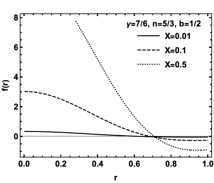
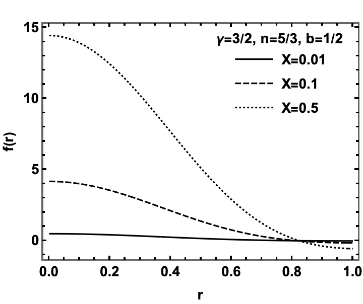
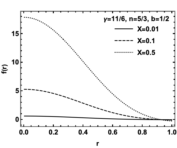
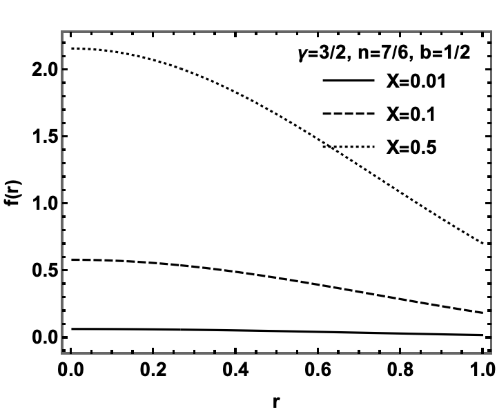
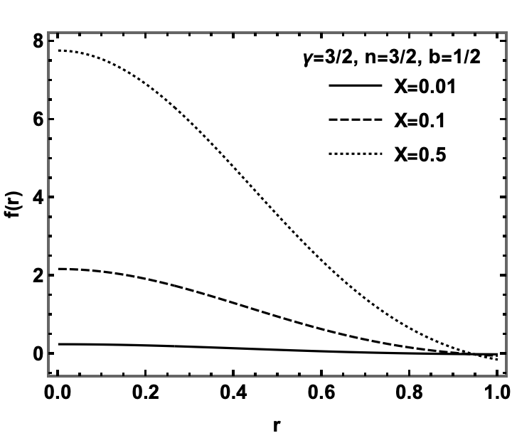
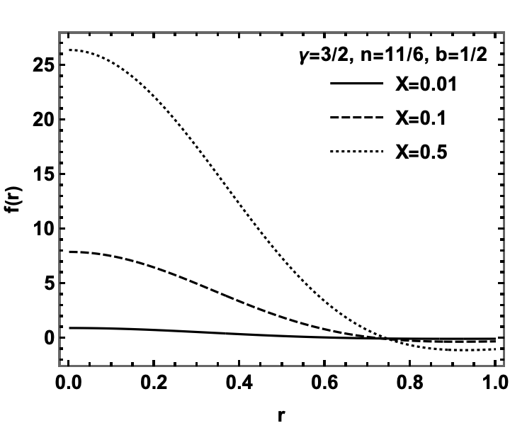
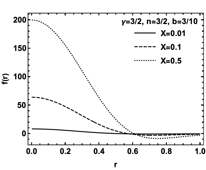

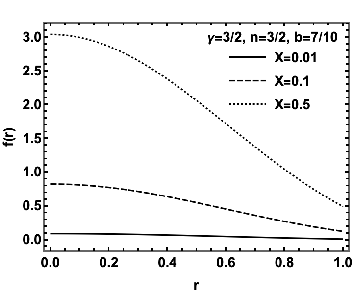
Depending on the sign of the function we can have a dynamically stable solution for , respectively an unstable one when , as explained in the previous section. We are mostly interested in finding the parameter space for solutions that have a stable behaviour. The fraction on the top row of Eq. (5.9) is always positive for our ranges of parameters. In particular, the relevant constraints on the parameters that lead to this conclusion are , , respectively . However, the remaining term can change sign and we cannot obtain clear analytical ranges for the free parameters in which the expression is either positive or negative. This term is a function of only, with no additional dependence on the star radius. For this reason, without loosing any generality, in Fig. 1 we plot the function as a function of , with , for three values of the compactness from low to intermediate and various sets of the remaining parameters. We first remark that, in many of the plots shown in Fig. 1, changes sign for values of somewhere between and . In order for a solution to be oscillatory, this function must be positive throughout the entire interval . As increases towards the surface of the star, in most cases decreases continuously and in many instances it also becomes negative. There are a few exceptions in which after decreasing to a minimum negative value, the function starts to increase again near the surface, however, for our choice of parameters it remains below zero. Having in mind the majority of the cases for which the function continues to decrease all the way to the star’s surface, it is interesting to analyse the parameter space for which the function is positive at . This is a fairly good indicator for finding the ranges of parameters for which the stars are dynamical stable. Considering that in some cases the function has a minimum and then starts to increase again, after picking a parameter set, the stability of the star needs to be evaluated in the entire volume from the center to its surface. At , the expression from (5.9) simplifies to
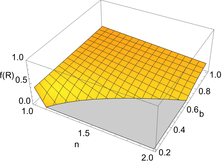
| (5.10) |
Fig. 2 shows a set of three dimensional plots for stars with a compactness value of . Again, without loosing any generality, we use . In each plot one of the three remaining free parameters , , respectively takes (increasing) discrete values, while the other two parameters span their entire allowed ranges. The plots show the regions in which is positive. The top panels show that as the Gaussian width increases, the ranges of and for which is positive also increase. This represents the expected behaviour, since in the large limit the density profile flattens out and ideally should reproduce the homogeneous density profile discussed in detail in Section 4. For uniform densities it was shown that the the quantity under the square root of (4.15) which is equivalent to , is always positive making these stars always stable.
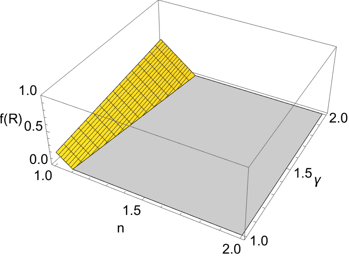
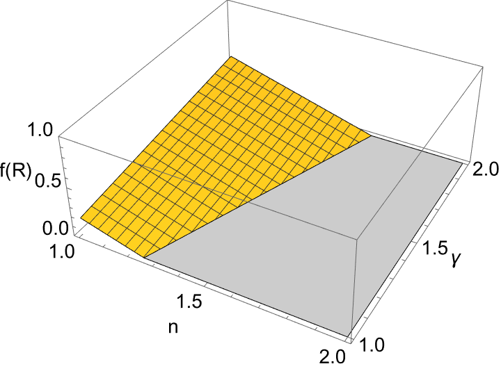
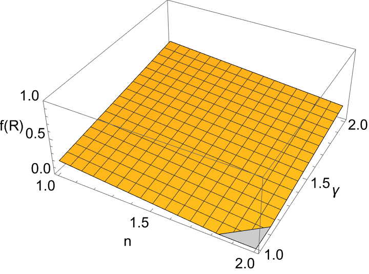
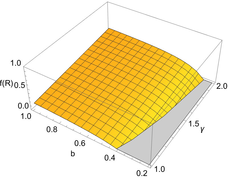
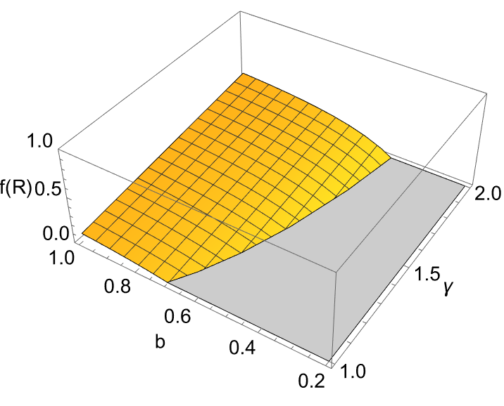
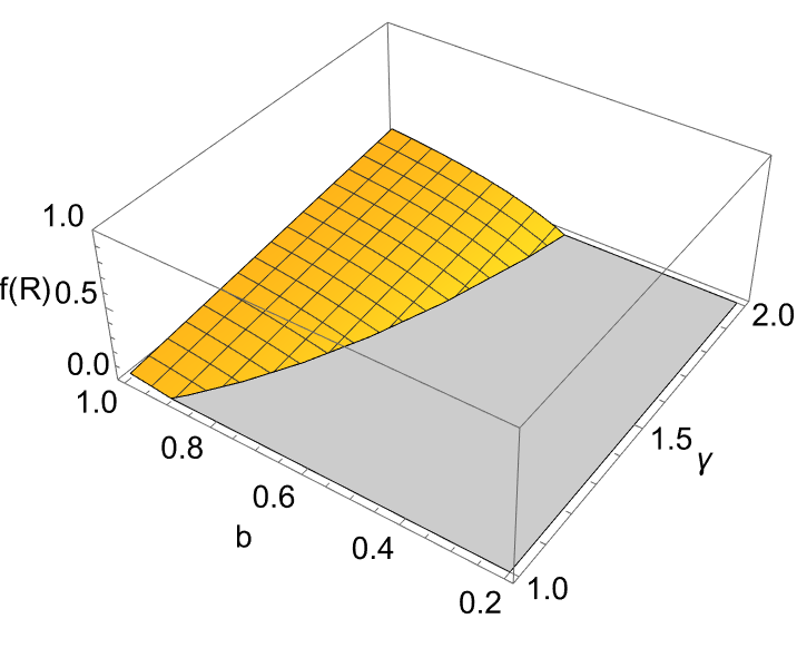
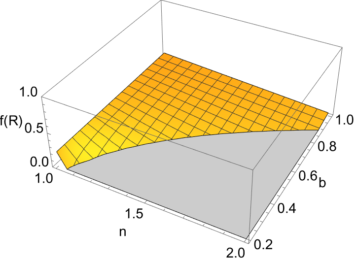
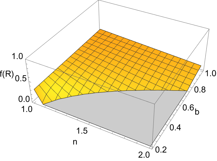
The middle panels show that, with the increase of the value of the polytropic index , larger values of the Gaussian width are required in order to for the solution to correspond to a star with stable oscillatory behaviour. Even if there is a smaller dependence on the value of the adiabatic index , for a constant index , as the value of decreases so does the interval of values for which the solutions are stable. One can do a similar analysis for the bottom plots in which the adiabatic index has discrete values. In this case one notices that as the value of increases a wider range of values of the gaussian width lead to stable solutions.
To summarise, depending on the values of all of the parameters from Eq. (5.10), they can lead to dynamically stable or unstable solutions. However, the strongest dependence is contained in the shape of the density profile.
6 Conclusions
In this article we analysed the dynamical stability of bootstrapped Newtonian stars following some homologous density perturbations which are also assumed to be adiabatic. The analysis was limited to stars of small or intermediate compactness, even if in the absence of a Buchdahl limit pressure can also sustain stars of large compactness in equilibrium. However, due to difficulties in finding approximate solutions for the potential inside high compactness sources, those cases are deferred for a future work.
Two separate cases were taken into consideration. In Section 4, stars with uniform densities were shown to be stable to the appearance of some adiabatic density perturbations such as the ones discussed above. These perturbations result in an oscillatory behaviour of the stars, regardless of their (low or intermediate) compactness , density value , or adiabatic index .
In Section 5 we analysed polytropes, more exactly polytropic stars with density profiles approximated by Gaussian-like functions as in Eq. (5.5). In this case it was shown that, depending on the parameters characterising these objects, both stable oscillating solutions and unstable solutions are possible. It was also observed that for the unstable cases, these instabilities appeared primarily in the outer layers of the star. Therefore, the next step was to evaluate the behaviour of the outermost layers of the bootstrapped Newtonian polytropic stars and conclude that when these layers had a stable oscillatory behaviour, it is highly likely for the entire object to be stable. We also pointed out that in order to be sure that a star characterised by a certain set of parameters is stable, one should evaluate its behaviour throughout the entire volume. When evaluating the stability of the outer layers, described by the function from Eq. (5.10), it was shown that wider (flatter) Gaussian density profiles led to stable solutions for greater ranges of the other remaining parameters such as the the adiabatic or polytroopic indices. When considering the dependence on the polytropic index, the parameter space for stable solutions was larger for smaller values of , while the opposite was true when considering the dependence on the adiabatic index .
To summarise, the bootstrapped Newtonian model can lead to stars that are dynamically stable following the appearance of some adiabatic density perturbations. What remains to be investigated is whether the same conclusions are reached for other types of perturbations such as thermal stability (which happens for instance when the star exceeds thermal equilibrium). It will be interesting to find out if the range of parameters for which we have thermal stability for bootstrapped Newtonian stars overlaps with the parameter space in which we found that these stars are dynamically stable. This analysis is deferred to some future works.
Acknowledgments
This research was supported by the Romanian Ministry of Research, Innovation and Digitalization under the Romanian National Core Program LAPLAS VII - contract no. 30N/2023.
References
- [1] R. Casadio, M. Lenzi and O. Micu, Phys. Rev. D 98 (2018) 104016 [arXiv:1806.07639 [gr-qc]].
- [2] R. Casadio, M. Lenzi and O. Micu, Eur. Phys. J. C 79 (2019) 894 [arXiv:1904.06752 [gr-qc]].
- [3] R. Casadio and O. Micu, Phys. Rev. D 102 (2020) 104058 [arXiv:2005.09378 [gr-qc]].
- [4] R. Casadio, M. Lenzi and A. Ciarfella, Phys. Rev. D 101 (2020) 124032 [arXiv:2002.00221 [gr-qc]].
- [5] R. Casadio, O. Micu and J. Mureika, Mod. Phys. Lett. A 35, (2020) 2050172 [arXiv:1910.03243 [gr-qc]].
- [6] R. Casadio, A. Giusti, I. Kuntz and G. Neri, Phys. Rev. D 103 (2021) 064001 [arXiv:2101.12471 [gr-qc]].
- [7] R. Casadio, I. Kuntz and O. Micu, Phys. Lett. B 834 (2022), 137455 [arXiv:2206.13588 [gr-qc]].
- [8] R. Casadio, I. Kuntz and O. Micu, Eur. Phys. J. C 82 (2022) no.7, 609 [arXiv:2205.04926 [gr-qc]].
- [9] R. L. Arnowitt, S. Deser and C.W. Misner, Phys. Rev. 116 (1959) 1322.
- [10] H. A. Buchdahl, Phys. Rev. 116 (1959) 1027.
- [11] A. D’Addio, R. Casadio, A. Giusti and M. De Laurentis, Phys. Rev. D 105 (2022) 104010 [arXiv:2110.08379 [gr-qc]].
- [12] R.C. Tolman, “Relativity, thermodynamics, and cosmology,” (Dover, 1987).
- [13] G. P. Horedt, “Polytropes: applications in astrophysics and related fields,” (Springer Netherlands, 2004).