Optimal Transport on the Lie Group of Roto-translations

Abstract

The roto-translation group SE(2) has been of active interest in image analysis due to methods that lift the image data to multi-orientation representations defined on this Lie group. This has led to impactful applications of crossing-preserving flows for image de-noising, geodesic tracking, and roto-translation equivariant deep learning. In this paper, we develop a computational framework for optimal transportation over Lie groups, with a special focus on SE(2). We make several theoretical contributions (generalizable to matrix Lie groups) such as the non-optimality of group actions as transport maps, invariance and equivariance of optimal transport, and the quality of the entropic-regularized optimal transport plan using geodesic distance approximations. We develop a Sinkhorn like algorithm that can be efficiently implemented using fast and accurate distance approximations of the Lie group and GPU-friendly group convolutions. We report valuable advancements in the experiments on 1) image barycenters, 2) interpolation of planar orientation fields, and 3) Wasserstein gradient flows on SE(2). We observe that our framework of lifting images to SE(2) and optimal transport with left-invariant anisotropic metrics leads to equivariant transport along dominant contours and salient line structures in the image. This yields sharper and more meaningful interpolations compared to their counterparts on $\mathbb{R}^{2}$.

62H35, 68U10, 90B06, 68T45, 68U99

1 Introduction and Background

1.1 The Roto-translation Group

Lie groups provide a potent mathematical framework for understanding geometric transformations and symmetries that frequently arise in many real-world applications. Lie group theory provides a natural foundation for expressing these symmetries and enhances the efficiency and interpretability of computational models that incorporate their mathematical structure. The Lie group SE(2) has been of particular interest in image processing. Firstly, it is natural to demand that any operation applied to the image (e.g. denoising, segmentation, feature extraction, etc.) has to be equivariant to a roto-translation of the image function. Simply put, operating on the image after a roto-translation or roto-translating the image after the operation must yield an identical output. Secondly, in many applications, it is desirable to identify one or more planar orientations at each 2D location in the image. This enables the effective processing of important image sub-structures with directional attributes like lines, edges, crossings, bifurcations, etc. For example, in the domain of medical image processing there is often a requirement of crossing preserving de-noising of images. Many of these images contain line structures having multiple crossings and bifurcations and we require that the denoising method preserve these structures [45, 16, 22]. Methods not accounting for such local orientation information often lack this property leading to distortionary results. Furthermore, medically significant line structures need to be spatially tracked leading to accurate measurements, which is useful for many further diagnoses. In such situations, the tracking algorithm must correctly identify and then move along the most cost-effective local orientation in order to extract the appropriate segment in that application.

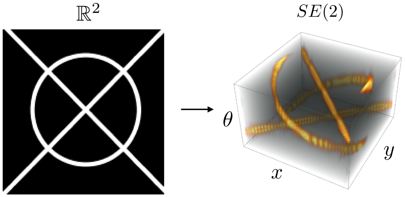
Figure 1: An orientation score transform (see Eq. 20) disentangles line structures due to lifting onto the Lie group SE(2). This is a useful property in many applications like image de-noising, geodesic tracking, equivariant deep learning, etc. In this paper, we use it for the barycentric interpolation of images using optimal transport as seen in the schematic in Fig. 2

This becomes especially critical at junctions that may yield multiple orientations and tracking on the image domain in $\mathbb{R}^{2}$ is typically insufficient to make the correct choice [13, 7, 77].

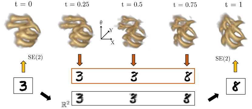
Figure 2: Barycenter interpolation in $\mathcal{P}(\text{SE(2)})$: To interpolate classical 2D images in $L^{2}(\mathbb{R}^{2})$ (in this case, an image of 3 and an 8), we first lift them to the space of probability measures $\mathcal{P}(\text{SE(2)})$ with operations involving invertible orientation scores (see Fig. 1 and equation Eq. 20). We then compute Wasserstein barycenters on that space (see Eq. 13) using linear weights indicated by $t$. Finally, we project the output back to $L^{2}(\mathbb{R}^{2})$ (by integration over $\theta$, cf. Eq. 21). We observe sharper and more meaningful interpolation in this process due to the left-invariant anisotropic metrics in SE(2) that yield a unique contour-concentrating behavior of the optimal transport. This is in contrast to isotropic transport in ${\mathbb{R}}^{2}$ where one observes significant mass splitting and leakage away from the main contours.

A common feature of orientation-aware methods that efficiently address these issues is that they lift the image data into the homogeneous space of positions and orientations. The lifting is usually done through an orientation score transform as we depict in Fig. 1 (see also [22, 31, 6, 16, 19]). The Lie group of roto-translations $\text{SE(2)}:=\mathbb{R}^{2}\rtimes\text{SO}(2)$ acts naturally on this space of positions and orientations $\mathbb{M}^{2}:=\mathbb{R}^{2}\times S^{1}$, which is also its principal homogeneous space. In fact, by fixing a reference position-orientation in $\mathbb{M}^{2}$ the two spaces can be identified with each other. The geometric algorithm is then applied in this lifted space, and finally, the processed orientation score is projected back yielding the output. Methods that follow this broad workflow are equivariant to roto-translations of the input by design. This workflow is also the backbone behind many successful roto-translation equivariant deep-learning architectures (called G-CNNs): [72, 8, 81] that are more efficient and need less training data. The computational machinery in all these methods indispensably use differential geometric structures like left-invariant Riemannian and sub-Riemannian geodesics, distances and kernels of the Lie group SE(2).

Despite these impactful applications, there has been little progress on the theory and applications of optimal transport problems in this domain. We report a relevant related work [44] that explores image morphing in the visual cortex using optimal transport. Functions in $\mathbb{R}^{2}$ are lifted onto this cortical space using Gabor filters parameterized by position, orientation, and scale. However, in our article, we uniquely exploit the SE(2) group structure (analytic distance approximations and group convolutions) to provide a scalable (Sinkhorn-like) algorithm. We apply our algorithm to orientation scores (constructed by ’all-scale’ cake wavelets), multitude of images, orientation fields, and to compute numerical solutions to PDEs. Finally, we provide new theoretical results as outlined in Section 1.3.

1.2 Optimal Transport on Geometric Domains

Optimal transport (OT) provides a principled and versatile approach to work with measures defined on very general spaces including Riemannian manifolds and SE(2). Among the many ideas coming from OT, we may mention mathematical tools to compare or interpolate between probability distributions. The prototypical example of an OT problem is the two-marginal Monge-Kantorovich assignment: given two Polish spaces $X_{1}$ and $X_{2}$ and given two probability measures $\mu\in\mathcal{P}(X_{1})$ and $\nu\in\mathcal{P}(X_{2})$, solve

(1) $$\inf\biggl{\{}\int_{X_{1}\times X_{2}}c(x_{1},x_{2})\mathrm{{d}}\pi(x_{1},x_{2})\;:\;\pi\in\Pi(X_{1}\times X_{2};\mu,\nu)\biggr{\}}$$

where $c:X_{1}\times X_{2}\mapsto\mathbb{R}^{+}$ is a lower semi-continuous cost function. The infimum runs over the set $\Pi(X_{1}\times X_{2};\mu,\nu)$ of coupling measures (usually called transport plans) on $X_{1}\times X_{2}$ with marginal distributions equal to $\mu$ and $\nu$ respectively. More generally, the problem can be multi-marginal as we introduce later on in Section 2.2.

Starting with the seminal formulations by Monge [58], Kantarovich [49] and later on by Brenier [17], the theoretical discourse on optimal transport is very extensive [79, 80, 69]. It has been shown to have rich and diverse connections to the theory of Partial Differential Equations (gradient flows [2], fluid mechanics [10], quantum chemistry [24, 12]), probability theory [2], and geometric analysis [54, 51] just to name a few. Many important PDEs like linear and non-linear diffusion and advection equations can be viewed as gradient flows on Wasserstein measure spaces. Such PDEs have a neurogeometrical significance when they are solved on SE(2) [63, 22, 42] and also have practical impact when combined with neural architectures [73] in deep learning.

In recent years, the development of efficient numerical approaches has opened the door to applying OT to numerous applications, notably in computer vision, image processing, computer graphics, and machine learning [38, 29, 53, 55, 50, 1]. Among the many numerical strategies that have been proposed in the literature, probably the most popular, and prominent direction consists in adding an entropic regularization term to the problem [26, 11, 74, 39], and considering an approximation of the measures by discrete measures via sampling or discretization on a grid. The discretization, and the additional entropy term lead to an approximation of the transport plan that can be computed using a fixed-point strategy, popularly known as the Sinkhorn algorithm. The Sinkhorn iterations have a linear convergence and only require convolutions with Gibbs kernels, thereby computing a smoothed version of the transport plan. For discretized geometric domains like triangulated meshes, point clouds, and graphs, a particularly widespread solution is the use of heat kernels [74, 78] in lieu of the distance-based Gibbs kernel. This avoids the need for computing distances and only evolving the heat equation which is in many applications numerically more straightforward on these domains. These advancements have been enormously beneficial in many applications: barycenters and shape interpolation [27, 25], generative models for machine learning [59, 4, 47], 3D shape registration and correspondence [36, 71, 61] to name a few. We refer to some excellent in-depth surveys in [62, 65, 15] for a more exhaustive list of the diverse applications of optimal transport. More closely related to the theme of this paper, optimal transport has also been studied for the interpolation of vector and tensor valued measures in [75, 64] as well as the rotation group SO(3) [67, 14]. As we demonstrate later in Section 5.3, orientation fields in $\mathbb{R}^{2}$ can be naturally lifted onto the homogeneous space of the Lie group SE(2) where we can employ anisotropic metrics for meaningful interpolation.

1.3 Contributions

In this paper, we formulate various optimal transport problems like the Wasserstein distance, barycenters, and gradient flows on the roto-translation group SE(2) by operating on its principal homogeneous space $\mathbb{M}^{2}=\mathbb{R}^{2}\times S^{1}$. In fact, most of our theoretical results can be generalized to any finite-dimensional Lie group, but we focus on numerical experiments involving SE(2) by lifting data from $\mathbb{R}^{2}$ to $\mathbb{M}^{2}$ (see Fig. 2). Our main contributions in this paper can be enumerated as follows:

1. Entropic OT on Lie groups: We extend the main result of [74] by demonstrating that entropic optimal transport on Lie groups can be solved with the Sinkhorn algorithm involving only group-convolutions with left-invariant kernels on the input distributions. We show that left-invariant costs lead to the invariance of the Wasserstein distance and equivariance of barycenters and gradient flow iterations for the same group actions on all input arguments of these applications.

2. Efficient approximation of the OT cost function $c$: The numerical cost of the Sinkhorn algorithm quickly becomes prohibitive when the number of discretization points increases, and when the evaluation of the cost function at each of the mesh points is not negligible. For OT problems formulated on general Riemannian manifolds like SE(2), the cost function $c$ is usually the geodesic distance between points of the discretization mesh in SE(2). Since it has no closed form, one needs to rely on fast approximations to solve the OT problem. In this paper, we address this issue by leveraging the logarithmic coordinates of SE(2) [9] to obtain a fast and accurate approximation of the Gibbs kernel. We make three experimental demonstrations:

   1. computing barycenters by lifting images to SE(2) (the conceptual flow is summarized in Fig. 2),

   2. interpolations of 2D orientation fields, and

   3. solving PDEs on SE(2) using Wasserstein gradient flows.

   Our experiments reveal favorable interpolations, aided by the lifting and anisotropic metrics that promote transport along salient line structures of the image. This helps reduce significant mass-splitting and promotes sharper results in the interpolations.

3. Theoretical results:

   1. We establish that for a wide class of Lie Groups, including SE(2), the right (and left) group action is generally not equal to the optimal transport map between a final distribution that is transformed by a group action of an initial distribution. However, such an equality statement does hold for Euclidean groups like $(\mathbb{R}^{n},+)$ and also for certain sub-Riemannian metrics and boundary-conditions on the Heisenberg group [3, Example 5.7].

   2. We derive corresponding bounds between Wasserstein distances constructed with the exact Riemannian distance and our distance approximations on the Lie group and also derive a similar result for the minimizing regularized optimal transport plans. This provides a theoretical justification for the use of the proposed approximations in practice.

1.4 Structure of the Article

In Section 2, we begin by giving a background on Lie groups, optimal transport, and details about our main numerical example SE(2). In Section 3 we explore the symmetries of optimal transport on Lie groups and additional results on the optimality of these symmetries. In Section 4 we formulate the entropic regularization for the OT problem in SE(2), and build a Sinkhorn algorithm, based on group convolutions and a distance approximation that can be efficiently implemented in this domain. We also show that error bounds on the approximation give rise to error bounds on the OT problems. Finally, in Section 5 we report the results of numerical experiments on images, orientation fields, and gradient flows on SE(2).

2 Background: Optimal Transport and Lie Groups

2.1 Lie Groups

We recall that a Lie group is a smooth manifold $G$ equipped with a group structure such that the group multiplication $\texttt{mult}:G\times G\to G$ given by $\texttt{mult}(g,h)=gh$ and the inverse $\texttt{inv}:G\to G$ given by $\texttt{inv}(g)=g^{-1}$ are smooth maps. The operations of left and right translation by a fixed element $g\in G$ are defined as the mappings

(2) $$L_{g}:G\rightarrow G,\;\;L_{g}(h)=gh\;\;\;\text{ and }\;\;\;R_{g}:G\rightarrow G,\;\;R_{g}(h)=hg.$$

Every $g\in G$ has an associated tangent space $T_{g}G$ which is the linear space spanned by all tangent vectors of curves passing through $g$. This tangent space has a dual space, denoted by $T^{*}_{g}G$, called the cotangent space. The tangent space at the identity element $e\in G$, $T_{e}G$, is called the Lie algebra. For a smooth map $\varphi:G\to N$ between $G$ and another smooth manifold $N$, the differential of $\varphi$ at $p\in G$ is a linear map $(\mathrm{d}\varphi)_{p}:T_{p}G\to T_{\varphi(p)}N$ from the tangent space of $G$ at $p$ to the tangent space $N$ at $\varphi(p)$. The image of $\mathrm{d}\varphi_{p}(\dot{p})$ of a tangent vector $\dot{p}\in T_{p}G$ under $\mathrm{d}\varphi_{p}$ is called the push-forward of $\dot{p}$ by $\varphi$. In the case $\varphi=L_{g}$ for a given $g\in G$, note that

$$(\mathrm{d}L_{g})_{p}:T_{p}G\to T_{gp}G.$$

Group Action, Invariance, and Equivariance

Given a group $G$ and a set $X$, a group action $A_{g}:X\to X$ is a mapping that satisfies $A_{g_{2}}\circ A_{g_{1}}=A_{g_{2}g_{1}}$ for all $g_{1},g_{2}\in G$ and $A_{e}=\text{id}_{X}$. We say that $G$ acts on $X$. Let $A_{g}:X\to X$ and $B_{g}:Y\to Y$ be two group actions. A function $\varphi:X\to Y$ is invariant (under $A_{g}$) if $\varphi\circ A_{g}=\varphi$. A function $\varphi:X\to Y$ is equivariant (w.r.t. $A_{g}$ and $B_{g}$) if $\varphi\circ A_{g}=B_{g}\circ\varphi$. In the specific case where the group action is the left-translation $L_{g}$ (or some corresponding derived notion) we speak of left-invariance, analogously, when the group action is the right-translation $R_{g}$ we speak of right-invariance.

Left Invariant Metric Tensor and Distance

As an additional structure, we endow the group $G$ with a metric tensor field $\mathcal{G}$, turning it into a Riemannian manifold which we denote by $(G,\mathcal{G})$. The metric tensor at a point $p\in G$ is a bilinear symmetric positive definite map $\mathcal{G}_{p}:T_{p}G\times T_{p}G\to{\mathbb{R}}$ which defines an inner product in the linear space $T_{p}G$. The mapping $p\mapsto\mathcal{G}_{p}$ is a smooth function of $p$. The metric tensor induces a natural way of defining a distance $d_{\mathcal{G}}$ on $G$ as

(3) $$d_{\mathcal{G}}(p,h):=\inf_{\begin{subarray}{c}\gamma\in PC([0,1];G)\\ \gamma(0)=p,\,\gamma(1)=h\end{subarray}}L(\gamma),\quad\text{ where }L(\gamma):=\int_{0}^{1}\sqrt{\mathcal{G}_{\gamma(t)}(\dot{\gamma}(t),\dot{\gamma}(t))}\mathrm{{d}}t,$$

where $\text{PC}([0,1],G)$ denotes the family of piece-wise continuously differentiable curves in $G$. We omit the subscript from $d_{\mathcal{G}}$ if it is clear from the context what metric is considered.

We say that the metric tensor is left-invariant iff for all $g,h\in G$ and $u,v\in T_{h}G$:

(4) $$\mathcal{G}_{h}(u,v)=\mathcal{G}_{L_{g}(h)}((\mathrm{d}L_{g})_{h}u,(\mathrm{d}L_{g})_{h}v).$$

When this property holds, it induces a left-invariant distance

(5) $$d_{\mathcal{G}}(p,h)=d_{\mathcal{G}}(L_{g}(p),L_{g}(h)),\quad\forall g,p,h\in G.$$

Left-invariant metrics play a key role because they allow for designing equivariant image processing operations.

2.2 Optimal Transport

Next, we introduce optimal transport problems posed on a Lie group $G$ with a left-invariant Riemannian metric $d$. We define the most classical problems such as the one of the Wasserstein distance, barycenters and gradient flows, and we discuss certain properties. Other common problems such as Gromov-Wasserstein discrepancies and barycenters could be introduced but we omit them in our presentation for the sake of brevity.

Let $\mathcal{M}(G)$ be the space of finite signed measures on $G$. Its positive cone and the set of probability measures are defined as

$$\mathcal{M}(G)_{+}\coloneqq\{\mu\in\mathcal{M}(G)\;:\;\mu\geq 0\},\;\;\mathcal{P}(G)\coloneqq\{\mu\in\mathcal{M}_{+}(G)\;:\;\mu(G)=1\}.$$

The OT problems that we consider in this work can be expressed as follows. Let $n\in\mathbb{N}$, and let $\mathcal{L}:\mathcal{P}(\mathcal{X})\rightarrow{\mathbb{R}}$ be a loss function with $\mathcal{X}=G^{n}=G\times\cdots\times G$. Given $K$ measures $\mu_{1},\dots,\mu_{K}\in\mathcal{P}(G)$ with $1\leq K\leq n$, the task is to solve

(6) $$\rho\coloneqq\inf_{\pi\in\Pi}\mathcal{L}(\pi),$$

where

(7) $$\Pi=\Pi(\mathcal{X};\mu_{1},\dots,\mu_{K})\coloneqq\{\pi\in\mathcal{P}(\mathcal{X})\;:\;(\mathrm{proj}_{i})_{\#}\pi=\mu_{i},\quad 1\leq i\leq K\},$$

is the set of coupling measures having the collection of $\mu_{i}$’s as marginals. In the above formula, $\mathrm{proj}_{i}:\mathcal{X}\to G$ denotes the projection on the $i$-th component, and the push-forward measure $(\mathrm{proj}_{i})_{\#}\pi$ is the $i$-th marginal of $\pi$.

For a measurable map $T:G\rightarrow G$, and a measure $\mu\in\mathcal{P}(G)$ the push-forward measure $T_{\#}\mu\in\mathcal{P}(G)$ is defined by the relation

$$T_{\#}\mu(A)=\mu(T^{-1}(A))\text{ for all measurable }A\subseteq G,$$

where $T^{-1}(A)$ denotes the pre-image of $A$ under $T$. One important example of this will be the push-forward action of left-translations,

(8) $$(L_{g})_{\#}:\mathcal{P}(G)\rightarrow\mathcal{P}(G),\textrm{ given by }\ ((L_{g})_{\#}\mu)(A)=\mu(L_{g}^{-1}A),$$

which is a group action of $G$ on $\mathcal{P}(G)$. The following classical OT problems can be written in the above general form:

• Wasserstein distances: For $p\geq 1$, the Wasserstein space $\mathcal{P}_{p}(G)$ is defined as the set of probability measures $\mu\in\mathcal{P}(G)$ with finite moments up to order $p$, namely

  $$\mathcal{P}_{p}(G)\coloneqq\biggl{\{}\mu\in\mathcal{P}(G)\;:\;\int_{G}d^{p}(x,x_{0})\,\mathrm{{d}}\mu(x)\;<+\infty\biggr{\}},$$

  where $x_{0}\in G$ is a (arbitrary) reference point in $G$. Let $\mu$ and $\nu$ be two probability measures in $\mathcal{P}_{p}(G)$. The $p$-Wasserstein distance $W_{p}(\mu,\nu)$ between $\mu$ and $\nu$ is defined by

  (9) $$W_{p}(\mu,\nu)\coloneqq\left(\mathop{\inf}_{\pi\in\Pi(G\times G;\mu,\nu)}\int_{G\times G}d^{p}(x,y)\,\mathrm{{d}}\pi(x,y)\right)^{\frac{1}{p}}.$$

  The space $\mathcal{P}_{p}(G)$ endowed with the distance $W_{p}$ is a metric space, usually called $L^{p}(G)$-Wasserstein space (see [79] for more details). The $W_{p}$ distance Eq. 9 is an optimal transport problem of the form Eq. 6 with $n=K=2$, and a l.s.c. cost function $c(x,y)=d^{p}(x,y)$ giving rise to

  (10) $$\mathcal{L}^{W_{p}}(\pi)\coloneqq\int_{G\times G}d^{p}(x,y)\,\mathrm{{d}}\pi(x,y).$$

  Optimizers $\pi^{*}$ of Eq. 9 are called optimal transport plans. Under certain conditions on the marginals, see [80, Corollary 9.3], one can guarantee the existence of an optimal map $T^{*}$ such that $\pi^{*}=(Id\otimes T^{*})_{\#}\mu$, which implies that $T^{*}_{\#}\mu=\nu$.

• Barycenters: To approximate or interpolate measures, one often resorts to Wasserstein barycenters. Let $n\in\mathbb{N}^{*}$ and let

  $$\Sigma_{n}\coloneqq\Big{\{}\lambda\in\mathbb{R}^{n}\;:\;\lambda_{i}\geq 0,\,\sum_{i=1}^{n}\lambda_{i}=1\Big{\}}$$

  be the simplex in $\mathbb{R}^{n}$. We say that $\mathrm{Bar}(\mathrm{Y}_{n},\Lambda_{n})\in\mathcal{P}_{p}(G)$ is a barycenter associated to a given set $\mathrm{Y}_{n}=(\mu_{i})_{1\leq i\leq n}$ of $n$ probability measures from $\mathcal{P}_{p}(G)$ and to a given set of weights $\Lambda_{n}=(\lambda_{i})_{1\leq i\leq n}\in\Sigma_{n}$, if and only if $\mathrm{Bar}(\Lambda_{n},\mathrm{Y}_{n})$ is a solution to

  (11) $$\mathrm{Bar}(\mathrm{Y}_{n},\Lambda_{n})\in\operatorname*{arg\,min}_{\nu\in\mathcal{P}_{p}(G)}\sum_{i=1}^{n}\lambda_{i}W_{p}^{p}(\nu,\mu_{i}).$$

  Problem Eq. 11 can be written as an optimization problem of the form Eq. 6 by setting $\mathcal{X}=G^{n+1}$, $\Pi=\Pi(\mathcal{X};\mu_{1},\cdots,\mu_{n})$ and taking the cost to be

  (12) $$c(\pi)=\sum_{i=1}^{n}\lambda_{i}\mathcal{L}^{W_{p}}\big{(}(\mathrm{proj}_{i}\otimes\mathrm{proj}_{n+1})_{\#}\pi\big{)},\quad\mathcal{L}^{\mathrm{Bar}}(\pi)=\int_{\mathcal{X}}c(\pi)\mathrm{d}\pi.$$

  We have that $\mathrm{Bar}(Y_{n},\Lambda_{n})=(\mathrm{proj}_{n+1})_{\#}\pi$. The case $n=2$ deserves some special attention. Let $\Lambda_{t}=(t,1-t)$ for $0\leq t\leq 1$, then we define the interpolation operator $\Phi_{t}:\mathcal{P}_{p}(G)\times\mathcal{P}_{p}(G)\rightarrow\mathcal{P}_{p}(G)$ as follows

  (13) $$\Phi_{t}(\mu,\nu):=\mathrm{Bar}\big{(}(\mu,\nu),\Lambda_{t}\big{)}.$$

  This operator is also called the displacement interpolation or McCanns interpolation between $\mu$ and $\nu$.

• Gradient flows: Given an initial condition $\mu_{0}\in\mathcal{P}(G)$, an energy functional $F:\mathcal{P}(G)\rightarrow{\mathbb{R}}$ and a timestep $\tau>0$, a discrete gradient flow evolution is defined as the time-marching

  (14) $$\mu_{k+1}\in\operatorname*{arg\,min}_{\nu\in\mathcal{P}(G)}W_{2}^{2}(\mu_{k},\nu)+\tau F(\nu),\quad\forall k\in\mathbb{N}.$$

  A single iteration is also reffered to as a JKO step, see [48], and can be written in the form of Eq. 6 by taking

  (15) $$\mathcal{L}^{GF}(\pi)=\mathcal{L}^{W_{p}}(\pi)+F((\mathrm{proj}_{2})_{\#}\pi),$$

  and $\Pi=\Pi(\mathcal{X};\mu_{k})$. The second marginal of $\pi$ plays the role of $\nu$ in Eq. 14.

2.3 The Special Euclidean group

Our main Lie group of interest is the three dimensional Special Euclidean group $\text{SE}(2)$ of all rigid body motions (or roto-translations) of ${\mathbb{R}}^{2}$. It is defined as the semi-direct product of ${\mathbb{R}}^{2}$ and $\text{SO}(2)$, $\text{SE}(2)={\mathbb{R}}^{2}\rtimes\text{SO}(2)$. We write $g=(x,R)\in\text{SE}(2)$, with $x\in{\mathbb{R}}^{2},\,R\in\text{SO}(2)$, and define group multiplication

(16) $$g_{1}g_{2}\coloneqq(x_{1}+R_{1}x_{2},R_{1}R_{2}),\quad\forall g_{1}=(x_{1},R_{1}),g_{2}=(x_{2},R_{2})\in\text{SE(2)}.$$

and with inversion given by $g^{-1}=(-R^{-1}x,R^{-1})$. The group $\text{SE}(2)$ acts naturally on ${\mathbb{R}}^{2}$:

(17) $$g\triangleright y=(x,R)\triangleright y=Ry+x,\textrm{ for all }y\in{\mathbb{R}}^{2},\,g\in\text{SE}(2).$$

Here we have used $\triangleright$ as a shorthand notation for the group action. We can identify any element $g\in\text{SE(2)}$ with $(x,y,\theta)\in{\mathbb{R}}^{2}\times{\mathbb{R}}/(2\pi{\mathbb{Z}})$, where we use the small-angle convention that ${\mathbb{R}}/(2\pi{\mathbb{Z}})=[-\pi,\pi)$. We call these coordinates the fixed coordinate system on SE(2). Then for $(x,y,\theta),(x^{\prime},y^{\prime},\theta^{\prime})\in\text{SE(2)}$ the group product becomes

$$(x,y,\theta)(x^{\prime},y^{\prime},\theta^{\prime})=(x+x^{\prime}\cos\theta-y^{\prime}\sin\theta\,,\,y+x^{\prime}\sin\theta+y^{\prime}\cos\theta\,,\,\theta+\theta^{\prime}\mod 2\pi),$$

and the identity element $e=(0,0,0)$. Given the basis $\{A_{1},A_{2},A_{3}\}=\{\partial_{x}|_{e},\partial_{y}|_{e},\partial_{\theta}|_{e}\}$ for the Lie algebra $T_{e}(\text{SE(2)})$, we get the so called left-invariant vector fields $\mathcal{A}_{i}|_{g}=({\rm d}L_{g})_{e}A_{i}$ via the pushforward of left translations:

$$(\mathcal{A}_{1})|_{g} =+\cos(\theta)\left.\partial_{x}\right|_{g}+\sin(\theta)\left.\partial_{y}\right|_{g}$$

$$(\mathcal{A}_{2})|_{g} =-\sin(\theta)\left.\partial_{x}\right|_{g}+\cos(\theta)\left.\partial_{y}\right|_{g}$$

$$(\mathcal{A}_{3})|_{g} =\left.\partial_{\theta}\right|_{g}$$

for all $g=(x,y,\theta)\in\text{SE(2)}$.

The left-invariant Riemannian distances on SE(2) that we consider are induced by left-invariant metric tensor fields characterized by

(18) $$\mathcal{G}_{g}(\mathcal{A}_{i}|_{g},\mathcal{A}_{j}|_{g})=\begin{bmatrix}w_{1}^{2}&0&0\\ 0&w_{2}^{2}&0\\ 0&0&w_{3}^{2}\end{bmatrix}$$

where $w_{i}>0$ are constant. We also define the spatial anisotropy $\zeta$ of the left-invariant metric tensor field $\mathcal{G}$ as

(19) $$\zeta\coloneqq\frac{\max(w_{1},w_{2})}{\min(w_{1},w_{2})}\in[1,\infty).$$

We say the metric is (spatially) isotropic if $\zeta=1$, and anisotropic otherwise. Lastly we need the Haar measure on SE(2), which up to a scalar constant coincides with the Lebesgue measure on ${\mathbb{R}}^{2}\times({\mathbb{R}}/(2\pi\mathbb{Z}))\equiv{\mathbb{R}}^{2}\times[-\pi,\pi)$ given by $\mathrm{{d}}g=\mathrm{{d}}x\mathrm{{d}}y\mathrm{{d}}\theta$.

2.3.1 Lifting and Projecting Images to and from Orientation Scores

In this paper, we focus on numerical examples that lift images $f\in L^{2}({\mathbb{R}}^{2})$ to orientation scores $U\in L^{2}(\text{SE(2)})$. We rely on the so-called orientation score transform defined as the mapping

$$\mathcal{W}_{\psi}:L^{2}(\mathbb{R}^{2}) \to L^{2}(\text{SE(2)})$$

(20) $$f \mapsto U(g)=(\mathcal{W}_{\psi}f)(g)\coloneqq\int_{{\mathbb{R}}^{2}}\psi(g^{-1}\triangleright x)\;f(x)\ \mathrm{{d}}x,\quad\forall g\in\text{SE(2)},$$

where $\psi\in(L^{1}\cap L^{2})({\mathbb{R}}^{2})$ is a chosen wavelet function.

Figure 1 gives an illustration of the transform. Its usefulness depends on the chosen wavelet $\psi$. It is worth mentioning that the orientation score transform is the only way to lift linearly onto the group SE(2) [5, Thm.1].

In this paper, we choose to employ cake wavelets (for details, we refer to [31, ch:4.6.1]). This choice results in a stable and interpretable lifting as can be seen in Fig. 1. Typically, no information is lost during the lifting from a function to its orientation score [31]. One can reconstruct bandlimited functions from the orientation score by a projection which we define as:

$$\mathrm{P}:L^{2}(\text{SE(2)}) \to L^{2}(\mathbb{R}^{2})$$

(21) $$U \mapsto\mathrm{P}(U)\coloneqq\int_{-\pi}^{\pi}U(\cdot,\theta)\;{\rm d}\theta.$$

In Fig. 2 the lifting operator (orientation score transform) is depicted by a yellow arrow, whereas the projection is indicated by an orange arrow.

Other possible lifting mechanisms include channel representations [41], tensor voting [46], or Gabor filters [44]. Such mechanisms are highly valuable if one wants to process orientation fields $(x,y)\mapsto v(x,y)\in[0,2\pi)$ (on images) [46] or robust orientation estimates [41, 37] rather than the scalar-valued images/densities $f$ themselves. We use one such lifting method for optimal transport over orientation fields in Appendix A.

2.3.2 The Importance of Equivariant Processing

We highlight an important connection between the lifting of images and the equivariant processing of orientation scores. We start by defining the following two natural group actions of $G=\text{SE(2)}$, $\mathcal{U}_{g}:L^{2}({\mathbb{R}}^{2})\to L^{2}({\mathbb{R}}^{2})$ and $\mathcal{L}_{g}:L^{2}(\text{SE(2)})\to L^{2}(\text{SE(2)})$:

(22) $$(\mathcal{U}_{g}f)(x):=f(g^{-1}\triangleright x),\quad\ (\mathcal{L}_{g}U)(h):=U(g^{-1}h).$$

Using $\mathcal{U}_{g}$ we can succinctly rewrite the orientation score transform as $(\mathcal{W}_{\psi}f)(g)=(\mathcal{U}_{g}\psi,f)$, where $(\cdot,\cdot)$ is the inner product on ${L^{2}({\mathbb{R}}^{2})}$. From the identity $(\mathcal{U}_{g}f_{1},\mathcal{U}_{g}f_{2})=(f_{1},f_{2})$ and the fact that $\mathcal{U}$ is a group representation one directly deduces:

(23) $$\mathcal{W}_{\psi}\circ\mathcal{U}_{g}=\mathcal{L}_{g}\circ\mathcal{W}_{\psi}\textrm{ for all }g\in G,$$

which means that lifting a roto-translated image is equivalent to left-translating the lift of the original image.

Consider an effective operator $\Upsilon:L^{2}(\mathbb{R}^{2})\to L^{2}(\mathbb{R}^{2})$ on the image domain that lifts images $f\in L^{2}(\mathbb{R}^{2})$, does some processing on the orientation score via an operator $\Phi:L^{2}(\text{SE(2)})\to(L^{1}\cap L^{2})(\text{SE(2)})$, and projects back:

(24) $$\Upsilon(f)\coloneqq(\mathrm{P}\circ\Phi\circ\mathcal{W}_{\psi})(f)=\int_{-\pi}^{\pi}(\Phi\circ\mathcal{W}_{\psi}f)(\cdot,\theta)\,{\rm d}\theta.$$

It is desirable for such an operator $\Upsilon$ to be roto-translation equivariant, that is

(25) $$\Upsilon\circ\mathcal{U}_{g}=\mathcal{U}_{g}\circ\Upsilon\textrm{ for all }g\in G.$$

This holds if the operator $\Phi$ on the orientation score is left-equivariant:

(26) $$\Phi\circ\mathcal{L}_{g}=\mathcal{L}_{g}\circ\Phi\textrm{ for all }g\in G.$$

One can quickly show this result using Eq. 23 (see [31, Thm.21] for further details).

In the following, our approach is to work with probability measures instead of functions at the level of SE(2). We thus build lifting operators $\widetilde{}\mathcal{W}_{\psi}:L^{2}(\mathbb{R}^{2})\to\mathcal{P}(\text{SE(2)})$, work with operators $\widetilde{\Phi}:\mathcal{P}(\text{SE(2)})\to\mathcal{P}(\text{SE(2)})$ inspired from OT for the processing, and project back via operators of the form $\widetilde{}\mathrm{P}:\mathcal{P}(SE)\to L^{2}(\mathbb{R}^{2})$. In a similar manner as for the approach with functions, if we want to guarantee roto-translation equivariance, we need to work with OT operators that are equivariant w.r.t. the group action defined in Eq. 8. For now we define

(27) $$(\widetilde{\mathcal{W}}_{\psi}(f))(A):=\frac{\int_{A}(\mathcal{W}_{\psi}f(q))_{+}{\rm d}q}{\int_{G}(\mathcal{W}_{\psi}f(q))_{+}{\rm d}q}$$

with $a_{+}=\max\{a,0\}$ for all measurable sets $A\subset\text{SE(2)}$. Now from Eq. 23 and left-invariance of the Haar measure it now directly follows that effective operator $\widetilde{\Upsilon}(f)\coloneqq(\mathrm{P}\circ\tilde{\Phi}\circ\widetilde{\mathcal{W}}_{\psi})(f)=\int_{-\pi}^{\pi}(\tilde{\Phi}\circ\widetilde{\mathcal{W}}_{\psi}f)(\cdot,\theta)\,{\rm d}\theta$, now with $\tilde{\Phi}:\mathcal{P}(\text{SE(2)})\to\mathcal{P}(\text{SE(2)})$, commutes with roto-translations if

$$(L_{g})_{\#}\circ\tilde{\Phi}=\tilde{\Phi}\circ(L_{g})_{\#}\textrm{ for all }g\in\text{SE(2)}.$$

Remark 2.1.

Later in Section 5, the lifting $\widetilde{}\mathcal{W}_{\psi}$ will map to two probability measures on SE(2): one will capture the positive components of $\mathcal{W}_{\psi}$ (like in (27)), and the other the negative components, as also done in [44]. We will treat each component with the same optimal transport parameter settings, and add them afterwards. Working with both components will be crucial to keep contrast and sharp edges as in Fig. 2.

3 Symmetries and Theoretical Properties

Consider the setting of Fig. 2 where we are interpolating between two images $f_{0},f_{1}\in L^{2}(\mathbb{R}^{2})$ by lifting them to measures $U_{0},U_{1}\in\mathcal{P}(\text{SE(2)})$, performing optimal transport there, and projecting back to $L^{2}(\mathbb{R})$. Similar to the discussions in Section 2.3.2, for the process

$$(f_{0},f_{1})\mapsto f_{t}:=P\circ\Phi_{t}(U_{0},U_{1}),\textrm{ with }U_{i}=(\widetilde{}\mathcal{W}_{\psi}f_{i}),\;t\in[0,1],\;i=0,1.$$

to be roto-translation equivariant we need the Wasserstein barycenter interpolation $\Phi_{t}$ on SE(2), recall Eq. 13, to be left-equivariant:

(28) $$\Phi_{t}((L_{g})_{\#}U_{0},(L_{g})_{\#}U_{1})=(L_{g})_{\#}\Phi_{t}(U_{0},U_{1})\textrm{ for all }g\in G,t\in[0,1].$$

This motivates looking at the general invariance/equivariance properties of the introduced optimal transport problems.

3.1 Invariance and Equivariance of Optimal Transport

Next we formulate the desired symmetries of each of the introduced optimal transport problems, and prove that they are satisfied.

Proposition 3.1.

Let $G$ be a Lie group with left-invariant metric $d$, then:

• The Wasserstein distance is invariant, i.e. for all measures $\mu,\nu\in\mathcal{P}(G)$ we have

  $$W_{p}((L_{g})_{\#}\mu,(L_{g})_{\#}\nu)=W_{p}(\mu,\nu).$$

• Wasserstein barycenters are equivariant, for all $\mu_{1},\dots,\mu_{N}\in\mathcal{P}(G)$ and all $\Lambda_{N}\in\Sigma_{N}$ we have

  $$\mathrm{Bar}(L_{g}\#\mathrm{Y}_{N},\Lambda_{N})=(L_{g})_{\#}\mathrm{Bar}(\mathrm{Y}_{N},\Lambda_{N}),$$

  where $L_{g}\#\mathrm{Y}_{N}=(L_{g}\#\mu_{1},\dots,L_{g}\#\mu_{N})$.

• If the gradient flow $\mathcal{L}^{GF}$ involves an invariant energy function $F:\mathcal{P}(G)\rightarrow{\mathbb{R}}$, then $\mathcal{L}^{GF}$ is invariant, and the whole evolution Eq. 14, that is $(\mu_{n})_{n\in{\mathbb{N}}}$, behaves equivariant.

Proof 3.2.

The proof relies on the fact that there is a bijection between $\Pi(\mathcal{X};\{\mu_{i}\}_{i=1}^{K}\}$ and $(L_{g})_{\#}\Pi\coloneqq\Pi(\mathcal{X};\{(L_{g})_{\#}\mu_{i}\}_{i=1}^{K}\})$. Consequently, if the loss function $\mathcal{L}$ from the general OT problem Eq. 6 is invariant, then we have invariance in the value of minimizers, and equivariance of the arg-minimizers. Therefore, it suffices to check that $\mathcal{L}^{W_{p}},$ $\mathcal{L}^{\mathrm{Bar}}$ and $\mathcal{L}^{GF}$ are invariant to prove our claim. For $\mathcal{L}^{W_{p}}$, let $(L_{g})_{\#}\pi\in(L_{g})_{\#}\Pi$. Then we easily see from left-invariance of the ground distance that

$$\mathcal{L}^{W_{p}}\big{(}(L_{g})_{\#}\pi\big{)}=\int_{G\times G}d^{p}(L_{g}(x),L_{g}(y))\,\mathrm{{d}}\pi(x,y)=\int_{G\times G}d^{p}(x,y)\,\mathrm{{d}}\pi(x,y)=\mathcal{L}^{W_{p}}\big{(}\pi\big{)},$$

so that indeed the cost function for the Wasserstein distance is invariant. The other statements are easily derived following similar lines.

We finish this section with a couple remarks:

• Many energy functionals $F$ for gradient flows satisfy the invariance assumption of Proposition 3.1. As an example, we may mention the class of “inner energy functionals” which take the form

  (29) $$F(\mu)=\begin{cases}\int_{G}f\left(\frac{\mathrm{{d}}\mu}{\mathrm{{d}}g}\right)\mathrm{{d}}g&\quad\text{ if }\mu\ll\mathrm{{d}}g\\ \infty&\quad\text{ else},\end{cases}$$

  where $f:G\rightarrow{\mathbb{R}}$ and $\frac{\mathrm{{d}}\mu}{\mathrm{{d}}g}$ denotes the Radon-Nikodym derivative of $\mu$ w.r.t. the Haar measure on $G$. Among the PDEs that they give rise to is for example the (non-linear) heat equation [80].

• With minimal technical additions, the results of Proposition 3.1 can also be carried out in the context of homogeneous spaces equipped with a left-invariant distance. As a matter of fact, we just need left-invariance of the cost function $c$ to guarantee equivariance of the whole process in general.

• We remark that the conclusion of Proposition 3.1 also applies to isotropic metrics on ${\mathbb{R}}^{2}$, i.e. optimal transport on $({\mathbb{R}}^{2},|\cdot|^{p})$ is also invariant/equivariant to roto-translations. However, the unique aspect of this property for SE(2) is that unlike ${\mathbb{R}}^{2}$, optimal transport with anisotropic metrics in SE(2) is also left-invariant. Anisotropic (or even sub-Riemannian) metrics in SE(2) relate to association fields [63, 22, 44, 9] from neurogeometry, and have a line completion behavior which is useful in many practical applications. This feature (important for contour-propagation and contour-perception) is unique to SE(2) and cannot be achieved with left-invariant metrics on ${\mathbb{R}}^{2}$.

3.2 Optimality of Right-Translated Measures

Here we study whether right-translations can be optimal transport maps of the Wasserstein metric, recall Eq. 9. Note that on a non-commutative group a fixed left-translation in general does not commute with left-translations, in contrast to right-translations, that do commute with all left-translations. The concrete question is:

For a given $\mu\in\mathcal{P}_{p}(G)$, let $\pi^{*}$ be the the optimal transport plan of $W_{p}(\mu,(R_{g})_{\#}\mu)$.
Is $\pi^{*}$ of the form $\pi^{*}=(\mathrm{Id},R_{g})_{\#}\mu$? In other words, is the transport map $T=R_{g}$ optimal?

We know there are a few cases in which this intuition holds, and we show that this result is not true in general for a wide class of Lie groups including $SE(2)$.

On the positive side, the result is true for $G={\mathbb{R}}^{n}$ (see for example Remark 2.19 in [65]). It is also true for certain right actions (right actions w.r.t. a specific sub-group) of $G=H(3)$ equipped with a specific sub-Riemannian structure as shown in [3]. However, we illustrate that this is not true in general by first building a counterexample in $SO(2)$.

Proposition 3.3.

Consider the Lie group $SO(2)$, identified with $\mathbb{R}/(2\pi\mathbb{Z})\equiv(0,2\pi]$ together with its left (or right) invariant metric $d$. Then we can find a measure $\mu$ and a group element $g$ such that $R_{g}$ (or $L_{g}$) is not the optimal transport map from $\mu$ to $(R_{g})_{\#}\mu$ (or $(L_{g})_{\#}\mu$) for the cost $d^{p}$ with $p\geq 1$.

Proof 3.4.

As the group $SO(2)$ is commutative left translations and right translations coincide. Let $0<\varepsilon\leq\pi/2$ be some positive constant and consider $\mu=\frac{1}{2}\delta_{\varepsilon}+\frac{1}{2}\delta_{2\pi-\varepsilon}$. Let $g=\pi$. We then have that $(R_{\pi})_{\#}\mu=\frac{1}{2}\delta_{\pi-\varepsilon}+\frac{1}{2}\delta_{\pi+\varepsilon}$.

It is clear that the cost associated to the transport map $R_{\pi}$ for the Monge formulation is $\pi^{p}$. However if we send the Dirac mass at $\varepsilon$ to the one at $\pi-\varepsilon$ and the one at $2\pi-\varepsilon$ to the one at $\pi+\varepsilon$, we get a cost strictly less than $\pi$, namely $(\pi-2\varepsilon)^{p}$. Hence we conclude that left translations cannot be optimal. We can apply the same reasoning to the right translation case.

Figure 3: An example of measure on $SO(2)$ and its right translation for which the optimal transport plan between them is not a right translation Proposition 3.3

Note that we could have built a similar example for functions with densities that are compactly supported on a sufficiently small interval. Also note that we could have taken a measure $\mu$ that was invariant under certain group actions, such as the uniform measure over $SO(2)$, but the example above has no such symmetries. We can leverage Proposition 3.3 to construct counter-examples for a much larger class of Lie groups.

Proposition 3.5.

Let $G$ be a Lie group that has a compact subgroup and $d$ a left invariant distance. Then we can find a measure $\mu$ and a group element $g$ such that $R_{g}$ (or $L_{g}$) is not optimal for the OT problem with cost $d^{p}$ with $p\geq 1$.

Proof 3.6.

By considering measures supported on the compact subgroup we assume w.l.o.g. that $G$ is compact. Every compact Lie group has a subgroup that is isomorphic to $SO(2)$. To see this, take some element in the Lie algebra and consider its generated one-parameter subgroup. If we take the closure of this subgroup we get an Abelian, compact, connected subgroup of $G$, which has to be isomorphic to a torus $\mathbb{T}^{k}$ for some $k>0$. This torus then has a subgroup, say $H$, isomorphic to $SO(2)$. Using the isomorphism $H\rightarrow SO(2)$ we can construct a left-invariant metric on $SO(2)$ such that the isomorphism is an isometry. We can then construct an example as in Proposition 3.3 to get an counter example on $G$.

As a consequence of Proposition 3.5, since SE(2) has a compact subgroup, we have the following corollary.

Corollary 3.7.

Left-actions on SE(2) are not left-invariant. Right actions are left-invariant. However both are not optimal maps in OT problems on SE(2) with left-invariant cost $d^{p}$ with $p\geq 1$.

Proof 3.8.

For all $g,h\in G$: $L_{g}\circ R_{h}=R_{h}\circ L_{g}\Rightarrow(L_{g})_{\#}\circ(R_{h})_{\#}\mu=(R_{h})_{\#}\circ(L_{g})_{\#}\mu$ for all $\mu\in\mathcal{P}_{p}(G)$. In a non-commutative Lie group like $G=\text{SE(2)}$ there exists $g,h\in G$ s.t. $L_{g}\circ L_{h}=L_{gh}\neq L_{hg}=L_{h}\circ L_{g}$ (where again we can take pushforwards). The rest follows by Proposition 3.5.

4 Entropic Regularization and Scaling algorithms

To solve OT problems of the form Eq. 6, we follow the approach based on adding an entropic regularization to the loss function (see, e.g., [26, 21]). For $G=\text{SE(2)}$, when the OT cost $c=d^{p}$, this leads to numerical schemes which boil down to computing group convolutions. The strategy is very computationally intensive, though, because Riemannian distances in SE(2) do not come in close form, and estimating them is an expensive operation. We leverage distance approximations that come in close form to make the scheme efficient (see [9]). This section summarizes the whole approach and provides an error analysis of the approximations that we use.

4.1 The Sinkhorn Algorithm

The entropic-regularized version of problem Eq. 6 reads

(30) $$\rho_{\varepsilon}=\inf_{\pi\in\mathcal{P}(\mathcal{X})}\mathcal{L}_{\varepsilon}(\pi),\quad\text{with }\mathcal{L}_{e}(\pi)\coloneqq\mathcal{L}(\pi)+\sum_{i=1}^{n}F_{i}((\mathrm{proj}_{i})_{\#}\pi)+\varepsilon\operatorname{KL}(\pi||\pi^{\text{ref}}),$$

where $\varepsilon\geq 0$ is the regularization parameter. The regularization term is the Kullback-Leibler (KL) divergence defined as

(31) $$\operatorname{KL}\left(\pi\;|\;\pi^{\text{ref}}\right)=\begin{cases}&\int_{\mathcal{X}}\log\left(\frac{\mathrm{{d}}\pi(x)}{\mathrm{{d}}\pi^{\text{ref}}(x)}\right)\mathrm{{d}}\pi(x),\quad\forall\pi\ll\pi^{\text{ref}},\text{ with }\pi,\,\pi^{\text{ref}}\in\mathcal{P}(\mathcal{X}).\\ &+\infty,\quad\text{else}.\end{cases}$$

In our scheme, we work with

$$\pi^{\text{ref}}=\otimes_{i=1}^{n}\alpha_{i},\quad\alpha_{i}\in\mathcal{P}(G)$$

as the reference measure where we choose the Haar measure $\mathrm{{d}}\alpha_{i}(g)=\mathrm{{d}}g$ for all $i=1,\dots,n$. This is done to guarantee invariance and equivariance properties in the scheme as we prove in Proposition 4.1. In Eq. 30, the functions $F_{i}:\mathcal{M}(G)\rightarrow{\mathbb{R}}$ are assumed to be proper, lower-semi-continuous and convex. They encode marginal constraints, or constraints of other nature. The regularization term makes the problem strongly convex, and guarantees uniqueness of a minimizer $\pi^{*}_{\varepsilon}$. One can show that as $\varepsilon\to 0$, $\pi^{*}_{\varepsilon}$ narrowly converges to the maximum entropy minimizer of the original problem (see [52, 18] for the proofs in the case of the Wasserstein distance, barycenters and gradient flows).

Using simple algebraic manipulations we can reformulate problem Eq. 30 as

(32) $$\inf_{\pi\in\mathcal{P}(\mathcal{X})}\varepsilon\operatorname{KL}\left(\pi\,||\,e^{-c/\varepsilon}\otimes_{i=1}^{n}\alpha_{i}\right)+\sum_{i=1}^{n}F_{i}((\mathrm{proj}_{i})_{\#}\pi).$$

We next recall the scaling algorithm to solve this problem (see [21] for its analysis). To simplify the presentation, we restrict the discussion to the case $n=2$. Given an initialization $b^{(0)}\in L^{\infty}(G)$ the algorithm repeats the following two operations until convergence:

(33) $$a^{(l+1)}=\frac{\text{prox}^{\operatorname{KL}}_{F_{1}/\varepsilon}\left(\mathcal{K}b^{(l)}\right)}{\mathcal{K}b^{(l)}},\;\;\;b^{(l+1)}=\frac{\text{prox}^{\operatorname{KL}}_{F_{2}/\varepsilon}\left(\mathcal{K}^{T}a^{(l+1)}\right)}{\mathcal{K}^{T}a^{(l+1)}},\quad l\in\mathbb{N},$$

were $\text{prox}^{\operatorname{KL}}_{F}$ denotes the proximal operator of $F$ with respect to the KL divergence, and is defined as

(34) $$\text{prox}^{\operatorname{KL}}_{F}(z)\coloneqq\operatorname*{arg\,min}_{s\in\mathcal{P}(G)}F(s)+\operatorname{KL}(s\;|\;z).$$

The application of $\mathcal{K}$ and $\mathcal{K}^{T}$ is defined as

(35) $$(\mathcal{K}b)(x)\coloneqq\int_{G}e^{-c(x,y)/\varepsilon}b(y)\;\mathrm{{d}}\alpha_{2}(y),\;\;\;(\mathcal{K}^{T}a)(y)\coloneqq\int_{G}e^{-c(x,y)/\varepsilon}a(x)\;\mathrm{{d}}\alpha_{1}(x).$$

We are looking for a fixed point of these iterations, say $a^{*},b^{*}$, after which we can recover the optimal coupling (as a density w.r.t. $\alpha_{1}\otimes\alpha_{2}$) by $\pi^{*}_{\varepsilon}(x,y)=a^{*}(x)e^{-c(x,y)}b^{*}(y)$ for all $(x,y)\in G\times G$. As an example, for the Wasserstein distance we can enforce that $\pi\in\Pi(\mathcal{X};\mu_{1},\mu_{2})$ by choosing for $i=1,\,2$,

(36) $$F_{i}(\nu)=\imath_{\{=\}}\big{(}\cdot|\mu_{i}\big{)}\coloneqq\begin{cases}0,&\text{ if }\nu=\mu_{i}\in\mathcal{P}(G)\\ +\infty,&\text{ else.}\end{cases},\qquad\text{prox}^{\operatorname{KL}}_{\imath_{\{=\}}\big{(}\cdot|\mu_{i}\big{)}}(z)=\mu_{i}\,.$$

Hence the (Sinkhorn) iterations read in this case (with point-wise division):

(37) $$a^{(l+1)}=\frac{\mu}{\mathcal{K}b^{(l)}},\;\;\;b^{(l+1)}=\frac{\nu}{\mathcal{K}^{T}a^{(l+1)}},\quad\forall l\in\mathbb{N}.$$

See Appendix C for a complete algorithm for the barycenter problem. We conclude this section by showing that the entropic-regularized versions of the optimal transport problems still maintain all invariance/equivariance properties from Proposition 3.1.

Proposition 4.1.

The entropic-regularized scheme preserves the same equivariant and invariant properties of the unregularized OT problems.

Proof 4.2.

Following the proof of Proposition 3.1, it suffices to show that $\pi\to\mathcal{L}_{\varepsilon}(\pi)$ is left-invariant. Since we showed this for the unregularized problems, it suffices to show left-invariance for the regularization term. We show this by

$$\begin{split}\operatorname{KL}\big{(}(L_{g_{0}})_{\#}\pi|\otimes_{i=1}^{n}\mathrm{{d}}h)&=\int_{\mathcal{X}}\log\left(\frac{\mathrm{{d}}(L_{g_{0}})_{\#}\pi}{\otimes_{i=1}^{n}\mathrm{{d}}h}(g)\right)\otimes_{i=1}^{n}\mathrm{{d}}h(g)\\ &=\int_{\mathcal{X}}\log\left(\frac{\mathrm{{d}}\pi}{\otimes_{i=1}^{n}\mathrm{{d}}h}(L_{g_{0}^{-1}}g)\right)\otimes_{i=1}^{n}\mathrm{{d}}h(g)\\ &=\int_{\mathcal{X}}\log\left(\frac{\mathrm{{d}}\pi}{\otimes_{i=1}^{n}\mathrm{{d}}h}(g)\right)\otimes_{i=1}^{n}\mathrm{{d}}h(g)=\operatorname{KL}\big{(}\pi|\otimes_{i=1}^{n}\mathrm{{d}}h).\end{split}$$

Finally, the $F_{i}$ are used to encode marginal constraints (except for the gradient flow), taking the form Eq. 36, and we can treat them the same way as the marginal constraints in Proposition 3.1. This proves that the regularized problem inherents the same symmetries as the unregularized problem.

4.2 Group Convolutions

When the cost function $c=d^{p}$ for a left-invariant distance $d$, the linear operation Eq. 35 becomes a group convolution that one can implement more efficiently than in the general case. The group convolution of a function $f:G\rightarrow{\mathbb{R}}$ with a kernel $K:G\rightarrow{\mathbb{R}}$ is defined by

$$(K*f)(g)\coloneqq\int_{G}K(h^{-1}g)f(h)\mathrm{{d}}h,\quad\forall g\in G,$$

Taking the reference measure $\pi^{\text{ref}}=\otimes_{i=1}^{n}\mathrm{{d}}h$ in the $\operatorname{KL}$ term, and defining

$$K(g)\coloneqq e^{-d^{p}(e,g)/\varepsilon},\quad\forall g\in G,$$

it follows by left-invariance of the distance map Eq. 5 that Eq. 35 can be written as convolutions

$$(\mathcal{K}b)(g)=\int_{G}e^{-d^{p}(g,h)/\varepsilon}b(h){\rm d}h=\int_{G}e^{-d^{p}(e,h^{-1}g)/\varepsilon}b(h){\rm d}h=(K*b)(g).$$

Note that the operator $\mathcal{K}$ and its adjoint $\mathcal{K}^{T}$ are equal because the symmetry of the Riemannian distance $d$ carries over to the cost $c=d^{p}$.

The convolutional structure opens the door to very efficient implementations of Eq. 35. SE(2) group convolutions are extensively used in geometric deep learning for image processing (e.g. [23, 82, 81, 8]) and robotics (e.g. [20]). Due to their widespread use in diverse applications, there have been many efficient implementations proposed (see [20, 43, 5]). Additionally, if the kernels have specific separability symmetries then further speed-ups can be expected [72, 40]. Unfortunately, in SE(2) such separability constraints are not generally applicable (if $w_{3}>0$, $w_{1}\neq w_{2}$). For a detailed overview of many steerable and non-steerable implementations with order complexities please refer [43, Tables 3.1 and 3.2]. In all of our experiments, we always work with non-steerable direct implementations.

4.3 Distance Approximations on SE(2)

Geodesic distances on SE(2) cannot be calculated in closed form, especially for anisotropic metrics which are of primary interest in this paper. In general, their estimation in practice is achieved using solutions to Eikonal PDE’s (see e.g. [56, 7, 70]). However, these approaches can become computationally expensive for large discretizations and high anisotropies. Instead, we now introduce analytic approximations that can be conveniently calculated in closed form and derive their numerical properties.

An analytic SE(2) distance approximation was introduced in [73], building upon standard approximation theory in Lie groups [68, 76] We sketch the general idea below. We start by noting that since $d$ is left-invariant, it suffices to approximate $d(e,g)$ for all $g\in\text{SE(2)}$ since in this case we can then evaluate $d(h,g)=d(e,h^{-1}g)$ for all $h,g\in G$.

For a Lie group with a surjective Lie group exponential $\exp:T_{e}G\to G$ we can, after choosing an appropriate subset of $T_{e}G$, make it injective. This way the Lie group logarithm $\log:G\to T_{e}G$, the inverse of the exponential, is well-defined, and we can use it to create a approximation of $d(e,g)$ in the following way.

The logarithmic distance approximation $\rho_{c}:G\to{\mathbb{R}}_{\geq 0}$ is defined as [73]:

(38) $$\rho_{c}(g)=\|\log g\|_{e}$$

where $\|\cdot\|_{e}:T_{e}G\to{\mathbb{R}}_{\geq 0}$ is the norm induced by $\mathcal{G}_{e}$. The calculation of $\rho_{c}$ is relatively easy and often expressible in closed form for many important Lie groups (for example matrix Lie groups), which means this approximation is generally applicable. The logarithmic approximation has the important global property that $d(e,g)\leq\rho_{c}(g)$ and one can show that it locally matches the distance in a precise sense explained further in the previously mentioned literature.

In [9] the logarithmic approximation $\rho_{c}$ on SE(2) is further refined to the half-angle approximation $\rho_{b}$ defined as

(39) $$\rho_{b}(g)\coloneqq\sqrt{(w_{1}b^{1}(g))^{2}+(w_{2}b^{2}(g))^{2}+(w_{3}b^{3}(g))^{2}}.$$

where $b^{i}:G\to{\mathbb{R}}$ are the half-angle coordinates, which for a given element $g=(x,y,\theta)$ can be computed as:

(40) $$\begin{array}[]{ll}\Big{(}b^{1}(g),b^{2}(g),b^{3}(g)\Big{)}&=\big{(}\,x\cos(\theta/2)+y\sin(\theta/2),\,-x\sin(\theta/2)+y\cos(\theta/2),\,\theta\,\big{)}.\end{array}$$

The approximative distance $\rho_{b}$ can be extended naturally to a metric-like structure on SE(2) by defining $\tilde{\rho}_{b}(g_{1},g_{2}):=\rho_{b}(g_{1}^{-1}g_{2})$. It is worth mentioning that this $\tilde{\rho}_{b}$ is not always strictly a metric on SE(2), as it is not guaranteed to satisfy the triangle inequality. However, we will refer to it as a distance purely because it serves as an approximation to it.

The logarithmic and half-angle approximation both have the same global symmetries as the exact distance $d(e,g)$ as shown in [9, Lemma 3]. However, in contrast to $\rho_{c}$, the approximation $\rho_{b}$ also has the desirable properties described in the following theorem.

Theorem 4.3 (Corollary 2, Lemma 7 from [9]).

The Riemannian distance $d=d_{\mathcal{G}}$ defined in Eq. 18, and the approximate distance $\rho_{b}$ defined in Eq. 39 are globally equivalent in the sense that

(41) $$\frac{1}{\zeta}d(e,g)\leq\rho_{b}(g)\leq\zeta d(e,g),\quad\forall g\in\text{SE(2)},$$

where $\zeta$ is the spatial anisotropy defined in Eq. 19. Furthermore, around any compact neighborhood $\Omega\subset\text{SE(2)}$ of the identity element $e$, we have that

$$d(e,g)^{2}\leq\rho_{b}(g)^{2}\leq\Big{(}1+\varepsilon(g)\Big{)}d(e,g)^{2},\quad\forall g=(x,y,\theta)\in\Omega,$$

where

$$\varepsilon(g):=\frac{\zeta^{2}-1}{2w_{3}^{2}}\zeta^{4}\rho_{b}^{2}(g)+C_{\Omega}|\theta|^{3}$$

and $C_{\Omega}\geq 0$ depends on $\Omega$.

4.4 Error analysis

Our resulting numerical algorithm involves two main approximations with respect to the original OT formulation: we introduce regularization, and we approximate $d$ with $\rho_{b}$. In this section, we theoretically analyze how much the final outputs deviate from the original OT solutions. We will focus on analyzing the Wasserstein distance problem. For this, recall that the original loss function to minimize is $\pi\mapsto\mathcal{L}^{W_{p}}(\pi)$ as defined in Eq. 10, and the value of the minimizer is $W_{p}(\mu,\nu)^{p}=\mathcal{L}^{W_{p}}(\pi^{*})$, where $\pi^{*}$ is the optimal transport plan. We denote the entropic-regularized version by $\pi\mapsto\mathcal{L}_{\varepsilon}^{W_{p}}(\pi)$, and the value of the minimizer is denoted by $W_{p,\varepsilon}(\mu,\nu)$. For our discussion, it will be useful to add the dependency on the underlying distance $d$ in the notation, so we will write these quantities as $\mathcal{L}^{W_{p},d}$ and $W_{p}^{(d)}(\mu,\nu)$ for the non-regularized formulation, and $\mathcal{L}_{\varepsilon}^{W_{p},d}$ and $W_{p,\varepsilon}^{(d)}(\mu,\nu)$ for the regularized versions respectively. We furthermore use the notation $\pi^{*}_{d,\varepsilon}$, $\pi^{*}_{\rho_{b},\varepsilon}$ for the regularized optimizers, and $\pi^{*}_{d,\varepsilon,n}$, $\pi^{*}_{\rho_{b},\varepsilon,n}$ for their Sinkhorn approximations after $n$ steps.

We prove in the next theorem that $W_{p}^{(d)}$ and $W_{p}^{(\rho_{b})}$ are equivalent in the sense that we can upper and lower bound one quantity with the other. The same result applies for the regularized versions.

Lemma 4.4.

For all $\mu,\nu\in\mathcal{P}(\text{SE(2)})$ it holds that

(42) $$\frac{1}{\zeta}W_{p}^{(d)}(\mu,\nu)\leq W_{p}^{(\rho_{b})}(\mu,\nu)\leq\zeta W_{p}^{(d)}(\mu,\nu)$$

and

(43) $$\frac{1}{\zeta}W_{p,\zeta^{p}\varepsilon}^{(d)}(\mu,\nu)\leq W_{p,\varepsilon}^{(\rho_{b})}(\mu,\nu)\leq\zeta W_{p,\zeta^{-p}\varepsilon}^{(d)}(\mu,\nu).$$

Proof 4.5.

Let $\pi\in\Pi(\mu,\nu)$. Using Eq. 41, we have that

$$\begin{split}W_{p,\varepsilon}^{(\rho_{b})}(\mu,\nu)^{p}&\leq\int\rho_{b}(h^{-1}g)^{p}\mathrm{{d}}\pi(h,g)+\varepsilon\operatorname{KL}(\pi|\mathrm{{d}}g\otimes\mathrm{{d}}g)\\ &\leq\zeta^{p}\left(\int d(h,g)^{p}\mathrm{{d}}\pi(h,g)+\frac{\varepsilon}{\zeta^{p}}\operatorname{KL}(\pi|\mathrm{{d}}g\otimes\mathrm{{d}}g)\right).\end{split}$$

Since this holds for all $\pi$, we can take the infimum over $\pi$ and the $p$-th root to get

(44) $$W_{p,\varepsilon}^{(\rho_{b})}(\mu,\nu)\leq\zeta W_{p,\zeta^{-p}\varepsilon}^{(d)}(\mu,\nu).$$

The other side of the bound can be derived in an analogous way. To get the result on the unregularized problem, one can set $\varepsilon=0$.

We next only consider $p=2$ and leverage recent results from [35] to estimate how much the optimal coupling $\pi^{*}_{d,\varepsilon}$ with exact distance $d$ differs from the optimal coupling $\pi^{*}_{\rho_{b},\varepsilon}$ with the distance approximation. We also compare it with $\pi^{*}_{\rho_{b},\varepsilon,n}$, the coupling that one can compute in practice after $n$ Sinkhorn iterations. For this, we need to introduce the following metric on $\text{SE(2)}\times\text{SE(2)}$,

$$\tilde{d}((g_{1},h_{1}),(g_{2},h_{2}))\coloneqq d(g_{1},g_{2})+d(h_{1},h_{2}),\quad\forall(g_{1},h_{1}),(g_{2},h_{2})\in\text{SE(2)}\times\text{SE(2)}.$$

Lemma 4.6.

Let $\mu,\nu\in\mathcal{P}(\text{SE(2)})$ be bounded and compactly supported measures, and let $\pi^{*}_{d,\varepsilon}$ and $\pi^{*}_{\rho_{b},\varepsilon}$ be the associated optimal regularized transport plans for the different costs. Then

$$W_{1}^{\tilde{d}}(\pi^{*}_{d,\varepsilon},\pi^{*}_{\rho_{b},\varepsilon,n})\leq\frac{C_{1}}{\varepsilon\sqrt{2}}\;\sup_{g=(x,y,\theta)\in S}\left(\frac{\zeta^{2}-1}{2w_{3}}\zeta^{4}\rho_{b}(g)^{2}+C_{2}|\theta|^{3}\right)d(e,g)^{2}+\frac{C_{3}}{\varepsilon}n^{-4},$$

where $C_{1}>0$ is a constant depending on $\mu,\nu$, $C_{2},\,C_{3}\geq 0$ are constants, and

$$S\coloneqq\{g\in\text{SE(2)}\,|\,g=h^{-1}k,h\in\text{{spt}}(\mu),k\in\text{{spt}}(\nu)\}.$$

Proof 4.7.

See Appendix B.

It follows from the bounds from Lemma 4.6 that $\pi^{*}_{d,\varepsilon}$ and $\pi^{*}_{\rho_{b},\varepsilon,n}$ are close only when the supports of $\mu$ and $\nu$ are concentrated and close to each other, which is something we can control using the discretization of the measures. The Lemma also reveals that the Sinkhorn iterations decay at a rate of $n^{-4}$, which suggests a rather fast convergence of the algorithm. One might even be able to prove faster convergence, see [34, 28], but this is not necessary for us, as the error we make in the approximate distance is already larger then the iteration error.

5 Numerical Experiments

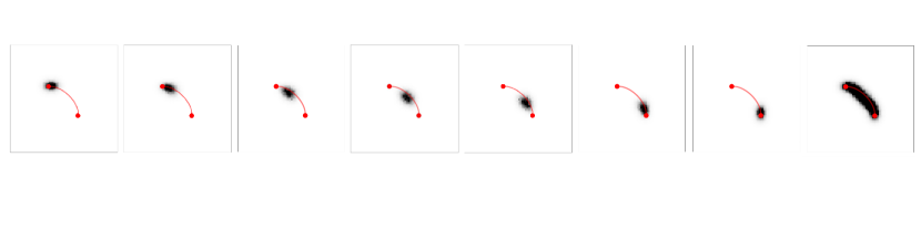
Figure 4: Tracing geodesics in SE(2): We interpolate between two Dirac masses using a anisotropic metric $(w_{1},w_{2},w_{3})=(1,5,2.5)$ in SE(2). The overlaid red curve is the exact sub-Riemannian geodesic between the two endpoints computed via analytic solutions from [32]. 1^st Row: Interpolation with Heat Diffusion in SE(2). 2^nd Row: Interpolation with the proposed half-angle distance approximation $\rho_{b}$ from equation ​Eq. 39. We can observe that the transport from our distance approximation is more accurate to the analytic solution in comparison to the analogous solution with Heat Diffusion. Columns 1-7: Spatially projected SE(2) interpolations on ${\mathbb{R}}^{2}$. Column 8: A cumulation of columns 1-7 showing the path that was traced. See Fig. 11 for an additional example.

We now report the results from the numerical implementation of our method for different applications. We apply the Sinkhorn algorithm with a SE(2) group convolution together with a Gibbs kernel made from the half-angle distance approximation $\rho_{b}$. We use the SE(2) group convolution implementation from the publicly available LieTorch package in [73]. All the results are based on the results from Section 4 leading to the SE(2) Wasserstein barycenter algorithm outlined in Appendix C. We report some additional examples in Appendix D.

5.1 Barycentric Interpolation with Synthetic Examples on SE(2)

We first validate our method by tracing the path obtained from a 2-Wasserstein interpolation of point masses in Fig. 4. We discretize SE(2) into a volume of $64\times 64\times 16$ by discretizing the spatial X-Y plane $[0,1]\times[0,1]$ into a $64\times 64$ grid and $\theta\in[0,2\pi)$ into 16 orientations.

We place two point masses at $g_{1}=(0.375,0.625,\theta=0^{\circ})$ and $g_{2}=(0.625,0.375,\theta=90^{\circ})$. We are particularly interested in tracing geodesics obtained under high-anisotropies or near sub-Riemannian conditions on SE(2). In this experiment, we validate a well-known result in OT: that the barycenter between two measures, recall Eq. 13, coincides with the McCann interpolation or displacement interpolation, which transports the mass of the measure along a geodesic, see for example [80, Section 7]. We compare the path of the interpolations with the true sub-Riemmanian geodesic. The overlaid red curve in Fig. 4 is computed with exact analytic formulas in [57, 32]. With increasing spatial anisotropies, Riemannian geodesics rapidly converge to the sub-Riemannian geodesics [33] where exact solutions are available. We compare the output of entropy-regularized Wasserstein interpolation with:

1. Solving Anisotropic Heat Diffusion on SE(2). This approach is a dominant paradigm for computing entropic OT on geometric domains (see [74]).

2. Our distance approximation $\rho_{b}$ with logarithmic coordinates from equation Eq. 39.

As we see in Fig. 4 the entropic-regularized 2-Wasserstein interpolation with $\rho_{b}$ very closely follows the exact geodesic. We observe that in this case it is numerically more accurate than the solution with anisotropic heat diffusion. This could be because optimal transport via the classical heat diffusion builds upon Varadan’s theorem [78] and hence requires very small time steps for high accuracy. In Fig. 11 we report an additional challenging example for tracing a sub-Riemannian geodesic with our algorithm.

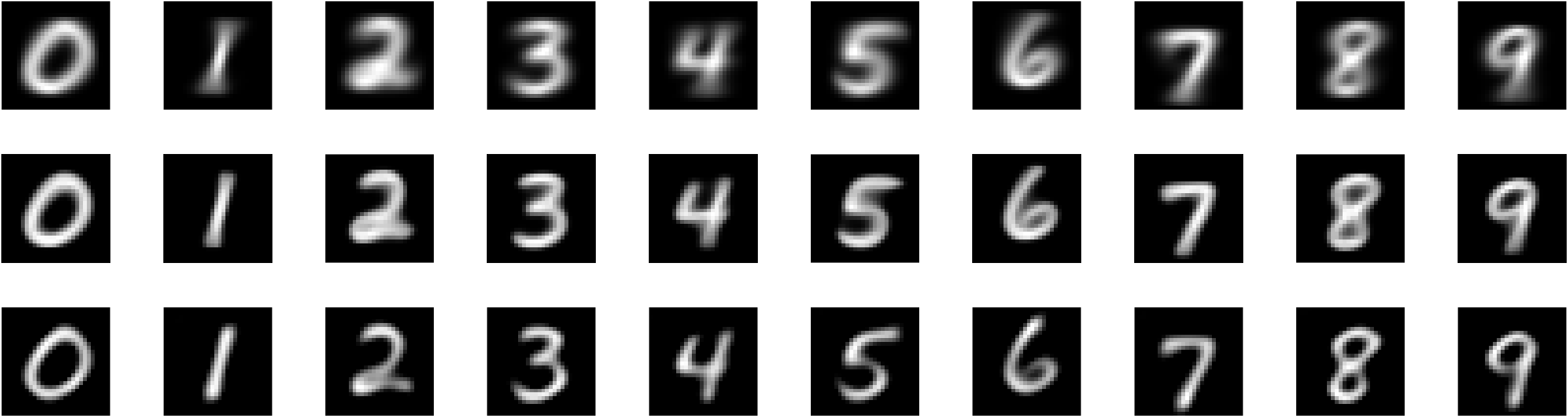
(a)

Figure 5: Average barycenters of all ($\sim 6000$ images per class) images from the MNIST dataset. 1^st Row: $L^{2}$ barycenter of all images per class - L2R . 2^nd Row: 2-Wasserstein barycenter in $\mathbb{R}^{2}$ - WR , 3^rd Row: 2-Wasserstein barycenter in SE(2) - WG . WG shows sharper interpolations in comparison with its counterparts on $\mathbb{R}^{2}$.

5.2 Barycentric Interpolation of Images with Lifting to SE(2)

Setting

We compute barycentric averages of images having shapes represented as 2D contours and line structures. We report qualitative results from 2 datasets that were particularly valuable in this setting: MNIST [30] and the QuickDraw. MNIST is the well known database of handwritten digits 0-9, with $\sim 6000$ images per class. Quickdraw is also a diverse database of doodles made by many people over the internet for different object classes.

We compare the following barycenters:

• Barycenters in the linear space $(L^{2}(\mathbb{R}^{2}),\|\cdot\|_{2})$,

• Barycenters in $W_{2}({\mathbb{R}}^{2})$ with entropic regularization and Euclidean distance $\|\cdot\|_{2}$ in $\mathbb{R}^{2}$,

• Barycenters in $W_{2}(\text{SE(2)})$, with entropic regularization and $\rho_{b}$ as a distance approximation in SE(2). This approach requires lifting the images from $L^{2}(\mathbb{R}^{2})$ to $\mathcal{P}_{2}(\text{SE(2)})$, and projecting back to $L^{2}(\mathbb{R}^{2})$ before and after the barycenter computation. These operations correspond to the operator $\widetilde{}\mathcal{W}_{\psi}$ in Section 2.3.2. We next explain how we have built them in practice in the next subsection.

Lifting and Projecting Images to and from Measures: Practical Aspects

To build a lifting $\widetilde{}\mathcal{W}_{\psi}:L^{2}(\mathbb{R}^{2})\to\mathcal{P}_{2}(\text{SE(2)})$, we take the orientation score transform $\mathcal{W}_{\psi}:L^{2}(\mathbb{R}^{2})\to L^{2}(\text{SE(2)})$ introduced in Eq. 20 as a starting point. For a given image $f\in L^{2}(\mathbb{R}^{2})$, the lifted image $\mathcal{W}_{\psi}(f)$ is not a probability measure because it may take on negative values. They are problematic for our purposes but they play a crucial role in accurate image recovery. The first idea to fix the issue would consist on working with the absolute value. However, this option did not work in our experiments, and its failure is connected to the loss of the sign in the value of the orientation scores.

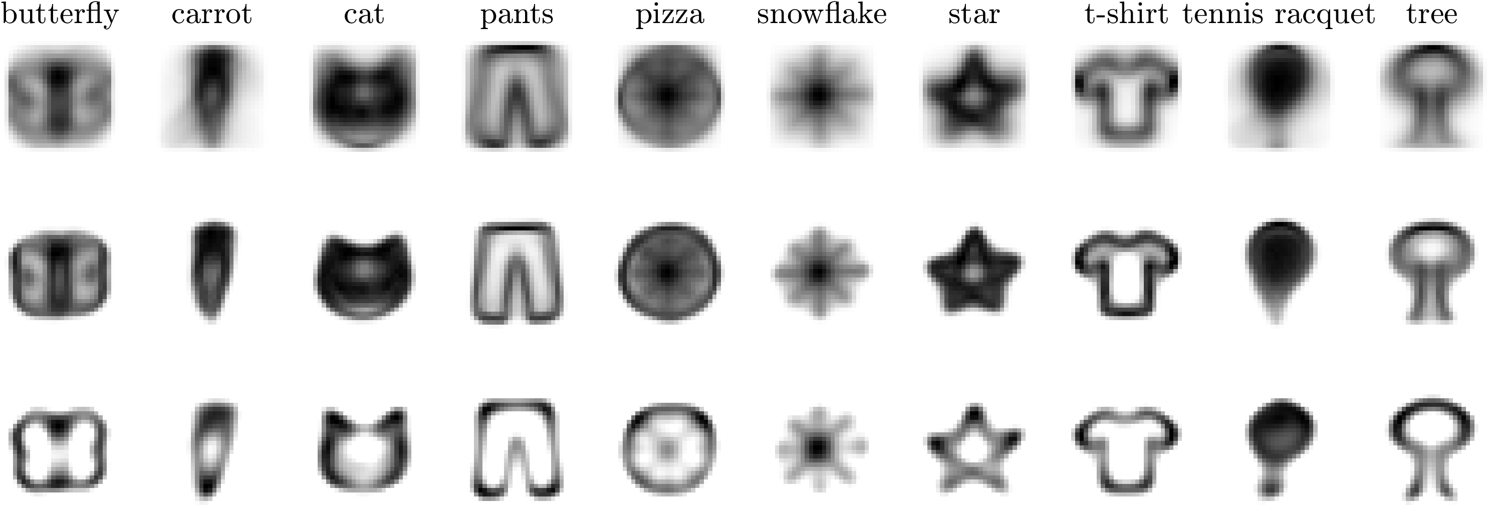
(a)

Figure 6: Average barycenters of ($\sim 6000$ images per class) images from the QuickDraw dataset. 1^st Row: $L^{2}$ barycenter of all images per class - L2R . 2^nd Row: 2-Wasserstein barycenter in $\mathbb{R}^{2}$ - WR , 3^rd Row: 2-Wasserstein barycenter in SE(2) - WG . WG shows sharper interpolations in comparison with its counterparts on $\mathbb{R}^{2}$.

Motivated by a similar construction from [44], we address this issue in practice by splitting the orientation scores into their respective positive and negative components and applying OT tools on them independently. For example, for computing WG between two images (recall Fig. 2) we do the following:

1. Lift images $f_{0},f_{1}\in L^{2}(\mathbb{R}^{2})$ to their scores $U_{0}=\mathcal{W}_{\psi}(f_{0})$ and $U_{1}=(\mathcal{W}_{\psi})(f_{1})$ (see Eq. 20).

2. Compute the positive and negative components of the scores:
   $\{U_{k}^{+},U_{k}^{-}\}:=\{\max\{U_{k},0\},-\min\{U_{k},0\}\geq 0\}$ for $k\in\{1,2\}$
   We normalize the output to sum up to 1 and therefore, we obtain measures $U_{k}^{\pm}\in\mathcal{P}_{2}(\text{SE(2)})$ for $k=1,2$

3. Compute the SE(2) Wasserstein barycenters $\Phi_{t}(U_{0}^{+},U_{1}^{+})$ and $\Phi_{t}(U_{0}^{-},U_{1}^{-})$, using the interpolation operator Eq. 13, and $\rho_{b}$ for the distance approximation. Proposition 4.1 guarantees that this step is left-equivariant: $\Phi_{t}(\mathcal{L}_{g}U_{0}^{\pm},\mathcal{L}_{g}U_{1}^{\pm})=\mathcal{L}_{g}\Phi_{t}(U_{0}^{\pm},U_{1}^{\pm})$.

4. Combine projections to get the image interpolant $b_{t}\in L^{2}(\mathbb{R}^{2})$:

   (45) $$b_{t}=\widetilde{}\mathrm{P}(U^{+}_{t},U^{-}_{t})\coloneqq\mathrm{P}(U^{+}_{t})-\mathrm{P}(U^{-}_{t}),\quad\forall t\in[0,1],$$

   where $\mathrm{P}$ is the projection operator defined in Eq. 21. Our projection $\widetilde{}\mathrm{P}$ ensures the interpolation property

   $$b_{t=0}=f_{0}\textrm{ and }b_{t=1}=f_{1}.$$

Since all steps are left-invariant, the whole procedure is left-invariant. Also, we emphasize that it is vital to use the same OT settings for the positive and negative components of the scores to ensure the respective interpolations are synced. In all our experiments we work with images that are also represented as densities $\mathcal{P}_{2}({\mathbb{R}}^{2})$. We threshold the projected output $b_{t}$ from Step 4 by keeping only the dominant positive response that is eventually normalized into $\mathcal{P}_{2}({\mathbb{R}}^{2})$ for WG as well as WR .

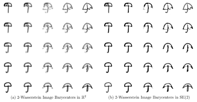
Figure 7: Comparing image barycenters in ${\mathbb{R}}^{2}$ and SE(2): We compute the barycenter between the 4 images at the corners, with linear weights in between. We select the regularization parameter such that the effective line thickness for both cases is approximately the same. WG promotes transport along line structures and hence, under this setting, we observe more undesirable mass splitting for WR in comparison to WG which shows a more meaningful interpolation. All images have been normalised to densities in ${\mathbb{R}}^{2}$ and we keep the same intensity range for a fair visualization. See Fig. 12 for an additional example.

Results

Figure 5 and Fig. 6 show the results for the MNIST and QuickDraw datasets respectively. Barycenters involve around $6000$ images per class. All input images were of dimension $28\times 28$ and for the SE(2) interpolation, we used 16 orientations for lifting and we chose the metric parameters setting $\zeta=1.5$. We normalize the results so that they are all visualized as probability densities on ${\mathbb{R}}^{2}$. Expectedly, WR gives a visually more coherent representation than the L2R and it does not suffer from the blurry artifacts present in the straightforward linear interpolation. However, we can see that WG is even sharper than WR and more representative of each class, yielding even more meaningful interpolations. This can be attributed to the lifting to the group and an-isotropic metrics that encourage mass movement over line structures.

In Fig. 7 we compare WR and WG more directly. We perform an interpolation of 4 images (at the corners) with linear weights. Again, we observe more meaningful interpolations for WG in comparison to WR .

5.3 Barycentric Interpolation of Orientation Fields

A natural application for optimal transport on SE(2) is the interpolation of orientation fields on ${\mathbb{R}}^{2}$, where one can associate a probability measure on SE(2) to an orienation field. As reported earlier, the interpolation of orientation fields using optimal transport has been explored in prior work, albeit on different geometries. [75] proposed the interpolation of two tangent vector fields defined on a triangulated 3D mesh and uses optimal transport as a way of matching the vector field singularities on this discrete surface. [64] proposed the extension of entropic optimal transport on matrix valued measures by using quantum-entropic-regularized optimization, which in practice leads to a modified Sinkhorn algorithm and is generalizable to arbitrary domains.

However, different from these methods, we highlight that orientation fields on Euclidean domains can be naturally lifted onto the corresponding roto-translation group and this can be used to exploit desirable aspects of the Lie group structure. We can therefore obtain a more convenient extension of [74] which allows for the efficient transport of dense orientation fields without explicitly needing to compute or store the OT coupling. In this setting, this is beneficial over a direct application of [64] which can lead to significant memory and computational requirements.

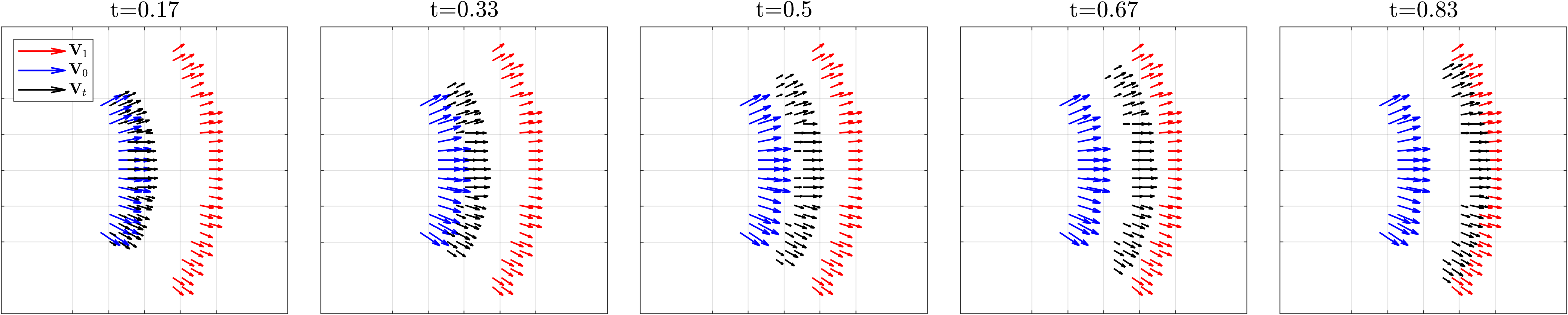
Figure 8: Entropic optimal transport with orientation fields on ${\mathbb{R}}^{2}$: An example of barycentric transport of orientation fields defined over $\mathbb{R}^{2}$. We lift a orientation field on ${\mathbb{R}}^{2}$ to the group SE(2) by assigning a magnitude and orientation to each location $(x,y)\in\mathbb{R}^{2}$. Using our method, we then compute the 2-Wasserstein barycenter of the two lifted measures and project back on the plane to visualize the interpolated orientation field. In this example we use a isotropic metric $(w_{1},w_{2},w_{3})=(1,1,1)$.

Lifting Orientation Fields: Practical Aspects

Given a vector field on ${\mathbb{R}}^{2}$ expressed in polar coordinates $v(\cdot)=|v(\cdot)|\;(\cos\psi(\cdot),\sin\psi(\cdot))^{T}$, with $\int_{{\mathbb{R}}^{2}}|v(x,y)|{\rm d}x{\rm d}y=1$, we lift it towards a regular probability measure $U\in\mathcal{P}(SE(2))$ via density:

(46) $$U(x,y,\theta)=\begin{cases}|v(x,y)|\frac{N}{2\pi}&\text{if }d_{S^{1}}(\psi(x,y),\theta)<\frac{\pi}{N}\\ 0&\textrm{else}\end{cases},$$

where $N$ denotes the number of orientations (sampled equidistantly at steps of $\frac{2\pi}{N}$). We project back by

(47) $$v(x,y)=\int_{-\pi}^{\pi}U(x,y,\theta)\;{\rm d}\theta\;\left(\begin{array}[]{c}\cos\psi^{*}(x,y)\\ \sin\psi^{*}(x,y)\end{array}\right)\ ,\textrm{ with }\psi^{*}(x,y)=\underset{\theta\in[-\pi,\pi)}{\operatorname*{arg\,max}}\;U(x,y,\theta)$$

This basic practical lifting replaces the Dirac distribution in Eq. 50 by uniform distributions over 0-th order B-splines. The construction Eq. 46 and reconstruction Eq. 47 can be generalized to advanced higher order B-spline orientation channels [37] but this is beyond the scope of this article.

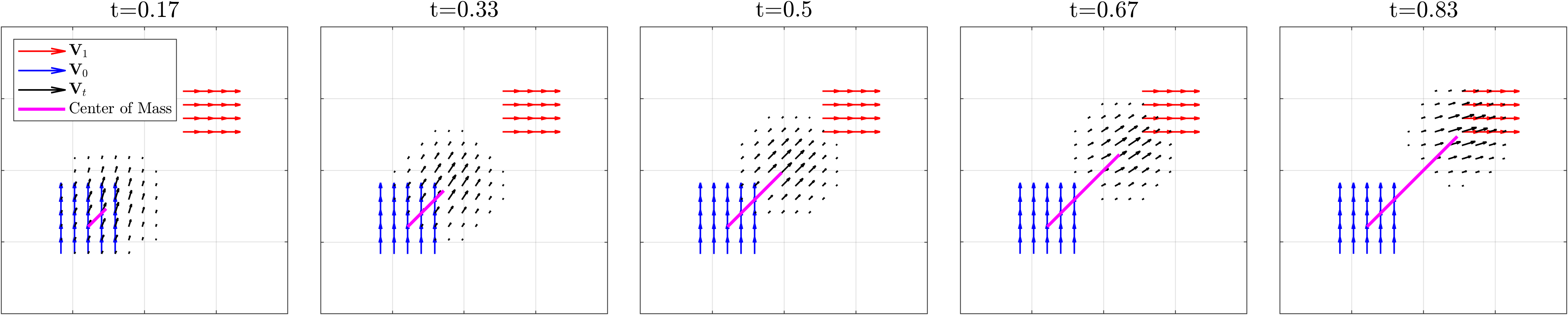
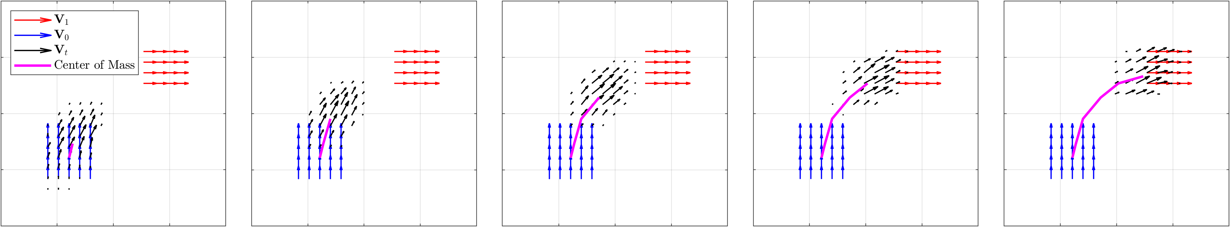
Figure 9: Another example similar to Fig. 8 where we interpolate a localized orientation field using different metrics in SE(2). (Top) Isotropic: $(w_{1},w_{2},w_{3})=(1,1,1)$ (Bottom) Anisotropic: $(w_{1},w_{2},w_{3})=(1,5,1)$. We highlight how choosing anisotropic metrics in SE(2) yield a natural u-curve and serves as a model for Reeds-Shepp car movement [33]

We can see an example of this for the localized vector fields displayed in blue and red in Fig. 8. The black arrows are obtained by lifting the two vector fields, interpolating the resulting measure in SE(2) and then projecting back to a vector field on ${\mathbb{R}}^{2}$. The result is a natural way of interpolating the two vector fields, both in location and direction. In Fig. 9 we can see a comparison between a (spatially) isotropic metric, i.e. $\zeta=1$ and an anisotropic metric, $\zeta\gg 1$. Depending on what the vector field represents, different spatial anisotropies can be used. For example, the highly anisotropic model can serve as a model for Reeds-Shepp car movement [33], modelling movement with certain curvature constraints.

This procedure can be extended to vector fields of any dimension $d$, by lifting them to the homogeneous space of positions and orientations $\mathbb{M}_{d}=SE(d)/SO(d\!-\!1)$, and performing optimal transport over these spaces. As mentioned previously, most of our developments carry over naturally to homogeneous spaces.

5.4 Wasserstein Gradient Flows for Line Completion

As a final example, we implement entropic Wasserstein gradient flows for solving PDEs. We use this setting to demonstrate a useful attribute of left-equivariant anisotropic SE(2) image processing: line-completion. We consider the images on the left of Fig. 10 as our guiding example. This image comprises a dominant line structure placed amid randomly located smaller line elements. We illustrate that we can complete and extract the main line by solving a non-linear diffusion equation in SE(2). For this, we take such an image and view it as an initial condition $\mu_{0}\in\mathcal{P}(G)$, with either $G=\text{SE(2)}$ or ${\mathbb{R}}^{2}$. We then compute the solution of

(48) $$\frac{\partial\mu}{\partial t}=\Delta_{\mathcal{G}}\mu^{m}$$

in a time-interval $[0,T]$, and with a left-invariant metric $\mathcal{G}$ on the Lie group $G$. The PDE in Eq. 48 represents the porous medium equation and presents a Wasserstein gradient flow structure [60] as per equation Eq. 15 with the functional

(49) $$F(\mu)=\frac{1}{m-1}\int_{G}\mu(g)^{m}\mathrm{{d}}g,$$

for $m>1$.

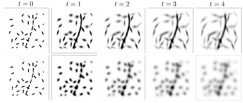
Figure 10: Gradient flow in SE(2) We implement a non-linear diffusion Eq. 48 with $m=5$ and with entropic Wasserstein gradient flow on both SE(2) (top row) and ${\mathbb{R}}^{2}$ (bottom row) using the same initialization. Different from ${\mathbb{R}}^{2}$, diffusions with left-invariant anisotropic metrics in SE(2) show a distinct line connectivity behavior as depicted in the evolutions. See Fig. 13 for an additional example.

We compute the solution for both groups ${\mathbb{R}}^{2}$ and SE(2) with $m=5$ by solving the discrete gradient flow time-marching Eq. 14 which we solve following the scheme introduced in [66]. On ${\mathbb{R}}^{2}$ we use the standard Euclidean metric, and on SE(2) we choose anisotropic metric parameters Eq. 18 to $(w_{1},w_{2},w_{3})=(1,3.1,1.4)$.

Diffusion in SE(2) with such high anisotropic metrics have a line completion behavior where dominant line structures get naturally connected in the evolution process. We can see this effect quite clearly in Fig. 10. We highlight that the anisotropy of SE(2) leads to a strong local orientation preference and this accumulates into the global line-connectivity behavior. In contrast, the isotropic diffusion in ${\mathbb{R}}^{2}$ does not yield the same result and the blur is uniform throughout the domain. Moreover, unlike SE(2), left-invariant anisotropic metrics in ${\mathbb{R}}^{2}$ have a global preference for direction that does not encourage line connectivity in every situation. We include an additional, slightly more challenging example in Fig. 13 to illustrate this point.

Figure 10 and Fig. 13 demonstrate the numerical implementation of the entropic Wasserstein gradient flow on SE(2) using our distance approximation $\rho_{b}$ and thus serve as an additional practical validation of our framework.

6 Conclusion

In conclusion, we build and apply an efficient computational framework for optimal transportation over the roto-translation group SE(2). We summarise the novel and impactful aspects of our contributions below:

1. We leverage distance approximations and group convolution operations toward efficiently extending the well-known Sinkhorn algorithm to SE(2). We theoretically justify our construction with Lemma 4.4 and Lemma 4.6. We numerically validate our approximation by tracing sub-Riemannian geodesics in Fig. 4 and report their fidelity to the analytical solutions.

2. We show more sharper and meaningful barycentric interpolations of images in Fig. 5, Fig. 6 and Fig. 7. These results are aided by the line-completing behavior of left-invariant anisotropic metrics on SE(2). This demonstrates the benefits of equivariant lifting-processing-projection of images onto SE(2) with optimal transport.

3. In Proposition 3.1 we derive the invariance and equivariance properties of optimal transport on SE(2). We theoretically establish that for a wide class of Lie Groups, including SE(2), the left/right group action is generally not equal to the optimal transport map between a final distribution that is a group action of an initial distribution in Proposition 3.5.

4. We show the Lie group SE(2) allows for an unique Riemannian and sub-Riemannian interpolation of orientation fields on ${\mathbb{R}}^{2}$ by lifting and projecting them from SE(2) in Fig. 8 and Fig. 9.

5. We apply an entropic Wasserstein gradient flow on SE(2) for the porous media equation. We show that the choice of left-invariant anisotropic metrics leads to the equivariant line completion behavior of the diffusion.

As exciting future work, we aim to extend to other Lie groups of practical significance like SO(3) and SE(3). In addition, developing accurate and efficient lifting and projection operations for Lie groups is also an avenue for prospective research in many practical applications where optimal transport could be applied.

Appendix A Idealized Lifts of Orientation Fields in ${\mathbb{R}}^{2}$ to SE(2)

Identify $S^{1}\equiv{\mathbb{R}}/(2\pi\mathbb{Z}\equiv[0,2\pi)$. Suppose we have an orientation field $\theta:\Omega\to[0,2\pi)$ with Lebesgue measure $\mu(\Omega)$ nonzero and finite. We can lift such an orientation field to a probability measure $U\in\mathcal{P}(\text{SE(2)})$ given by:

(50) $$U(x,y,\cdot)=\left\{\begin{array}[]{ll}\frac{1}{\mu(\Omega)}\delta_{\theta(x,y)}(\cdot)&\textrm{if }(x,y)\in\Omega\\ 0&\textrm{ else }\end{array}\right.$$

where we put a uniform distribution on $\Omega$ and at each position $(x,y)\in\Omega$ a Dirac measure w.r.t. angular variable $\theta$ centered at $\theta(x,y)$. Equation Eq. 50 can be interpreted as an idealized lift. One can reconstruct the orientation field $\theta:\Omega\to[0,2\pi)$ from the support of $U$ by

(51) $$\theta(x,y)=\theta\text{ if }(x,y,\theta)\in\text{supp }U\textrm{ for all }(x,y)\in\Omega.$$

In practice, however, we discretize both in space and orientation, and the intermediate probability measures obtained through the optimal transport have a support that is spread out over $\theta$ in general. This means this lift and projection above can not be used unadapted in our application. We explain a practical approximation in Section 5.3 that comfortably addresses this issue and we show meaningful interpolation of orientation field even with non-uniform spatial distributions (cf. equation Eq. 46). This approach could easily be generalized to B-spline orientation channels of a higher degree [37] than 0.

Appendix B Proof of Lemma 4.6

Proof B.1.

To prove Lemma 4.6, we first apply the triangle inequality:

(52) $$W_{1}^{\tilde{d}}(\pi^{*}_{d,\varepsilon},\pi^{*}_{\rho_{b},\varepsilon,n})\leq W_{1}^{\tilde{d}}(\pi^{*}_{d,\varepsilon},\pi^{*}_{\rho_{b},\varepsilon})+W_{1}^{\tilde{d}}(\pi^{*}_{\rho_{b},\varepsilon},\pi^{*}_{\rho_{b},\varepsilon,n}).$$

We then bound the two terms separately. For the first term, we wish to apply Proposition 3.12 from [35]. Since we assume $\mu,\nu$ are bounded and have compact support, we can apply the proposition with $p=\infty$ and $q=1$. We then have to check that we satisfy condition $I_{1}$ from [35]. This is true thanks to Lemma 3.10 from [35], again because we have compact and bounded marginals. Then proposition 3.12 from [35] gives us

(53) $$W^{\tilde{d}}_{1}(\pi^{*}_{d,\varepsilon},\pi^{*}_{\rho_{b},\varepsilon})\leq\frac{C_{1}}{\varepsilon\sqrt{2}}\left\lVert d^{2}-\rho_{b}^{2}\right\rVert_{L^{\infty}(\mu\otimes\nu)}.$$

We next apply Theorem 4.3 to derive:

$$\left\lVert d^{2}-\tilde{\rho}_{b}^{2}\right\rVert_{L^{\infty}(\text{{spt}}(\mu\otimes\nu))} \leq\sup_{(g,h)\in\text{{spt}}(\mu\otimes\nu)}|d(h,g)^{2}-\rho_{b}(h^{-1}g)^{2}|$$

$$=\sup_{g\in S}|d(e,g)^{2}-\rho_{b}(g)^{2}|$$

(54) $$\leq\sup_{g=(x,y,\theta)\in S}\left(\frac{\zeta^{2}-1}{2w_{3}}\zeta^{4}\rho_{b}(g)^{2}+C|\theta|^{3}\right)d(e,g)^{2}.$$

Plugging Eq. 54 into Eq. 53 yields the bound on the first term of Eq. 52. For the second term, Theorem 3.15 from [35] guarantees the existence of a constant $C_{3}\geq 0$ (which is independent of $\varepsilon$) such that

$$W_{1}^{\tilde{d}}(\pi^{*}_{\rho_{b},\varepsilon},\pi^{*}_{\rho_{b},\varepsilon,n})\leq\frac{C_{3}}{\varepsilon}n^{-4}.$$

Combining the two inequalities concludes the proof.

Appendix C SE(2) Wasserstein Barycenter Algorithm

We enumerate the SE(2) Wasserstein barycenter algorithm below. This is essentially identical to Algorithm 2 from [74] (and the scaling algorithm from [21] specified to the barycenter problem), but with necessary replacements (Section 4) for the Lie Group SE(2), i.e. using group convolutions and local distance approximations $\rho_{b}$.

function  SE(2)Wasserstein-Barycenter($\textrm{Inputs: }\{\mu_{i}\in\mathcal{P}(G)\}_{i=1}^{n};\textrm{Weights: }\{\lambda_{i}\}_{i=1}^{n}\in\Sigma_{n};\textrm{Regularization Parameter: }\varepsilon$) Notation

     $*\leftarrow\text{SE(2)}\textrm{ group convolution (ref. \lx@cref{creftype~refnum}{subsec:gconv})}$

     $\otimes\leftarrow\textrm{pointwise multiplication; }$ $\ominus\leftarrow\textrm{pointwise division}$ Initialization

     $v_{1},v_{2},\dotsm v_{n}\leftarrow\mathbf{1}$

     $w_{1},w_{2},\dotsm w_{n}\leftarrow\mathbf{1}$

     $K_{\varepsilon}\leftarrow e^{-\frac{\rho_{b}^{2}}{\varepsilon}}$ using Eq. 39 Sinkhorn Iterations with Iterated Bregman Projections

     for j = 1 … do

         $\mu\leftarrow\mathbf{1}$

         

         for i = 1 …n do

              $w_{i}\leftarrow\mu_{i}\ominus\{K_{\varepsilon}*v_{i}\}$

              $d_{i}\leftarrow v_{i}\otimes\{K_{\varepsilon}*w_{i}\}$

              $\mu\leftarrow\mu\otimes d_{i}^{\lambda_{i}}$

         end for

         

         for i = 1 …n do

              $v_{i}\leftarrow v_{i}\otimes\mu\ominus d_{i}$

         end for

     end for

     return $\mu$

end function

Appendix D Additional Examples

We report some additional numerical examples of our method below. We first report the tracing of a challenging s-curve geodesic in Fig. 11. Then, we show another example similar to Fig. 7 where we compare the barycenter interpolation between WR and WG on MNIST. Finally in Fig. 13 make another entropic Wasserstein gradient flow with a slightly more challenging line completion similar to Fig. 10.

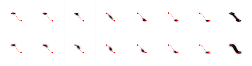
Figure 11: Tracing S-Curve Geodesics in SE(2): We interpolate between two Dirac masses $g_{1}=(0.375,0.625,\theta=0^{\circ})$ and $g_{2}=(0.625,0.375,\theta=0^{\circ})$ using anisotropic metric $(w_{1},w_{2},w_{3})=(1,7,2.5)$ in SE(2). The overlaid red curve is the exact sub-Riemannian geodesic between the two endpoints computed via analytic solutions from [32] with challenging extreme curvatures at the boundaries. 1^st Row: Interpolation with Heat Diffusion in SE(2). 2^nd Row: Interpolation with the version of the distance approximation $\rho_{b,com}$ [9, Eq.26]. The transport from the distance approximation is more accurate to the analytic solution in comparison to the analogous solution with Heat Diffusion. Columns 1-7: Spatially projected SE(2) interpolations on ${\mathbb{R}}^{2}$. Column 8: A cumulation of columns 1-7 showing the path that was traced.

Tracing S-Curve Geodesics in SE(2)

Sub-Riemannian geodesics come either as U or S shapes [57, 32] and we also demonstrate a challenging $S$-case with extreme curvatures at the boundary points in the same setup as Fig. 4. In [9] a series of distance approximations are studied, all of which were motivated by the logarithmic approximation we explain in Section 4.3. $\rho_{b}$ Eq. 39 is a very good distance approximation for spatial anisotropies (19) in the range $\zeta<5$. This was sufficient and yielded stable results in all our experiments in Section 5.

However, a further adjustment in the approximation should be made (with an automatic switch to the sub-Riemannian setting) if the spatial anisotropy is more extreme [9, Eq.26]. This is particularly relevant in the tracing of S-shaped sub-Riemannian geodesic in SE(2) with high curvature at the endpoints. As $\zeta\to\infty$ the Riemannian geodesics converge to more challenging sub-Riemannian geodesics, cf. [33, Thm.2]. In our experiments, $\zeta=7$ was large enough to verify the concentration of the optimal transport around an exact, high curvatures, sub-Riemannian S-shaped geodesics in Fig. 11.

Figure 12: Comparing image barycenters in ${\mathbb{R}}^{2}$ and SE(2): Another example similar to Fig. 7, with MNIST digits. The Images at the corners are interpolated using linear weights. Again, one observes a more meaningful interpolation with left-invariant anisotropic optimal transport in SE(2)

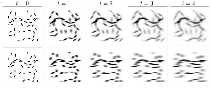
Figure 13: Gradient flow in SE(2) Another example similar to Fig. 10 where we implement a entropic Wasserstein gradient flow for the PDE Eq. 48 on both SE(2) (top row) and ${\mathbb{R}}^{2}$ (bottom row) using the same initialization. Here, we apply an anisotropic diffusion on SE(2) and ${\mathbb{R}}^{2}$. Note that OT with this metric on ${\mathbb{R}}^{2}$ is no longer equivariant to rotations. The rototranslation equivariant SE(2) flow (top row) shows a more distinct line completion behavior than the ${\mathbb{R}}^{2}$ flow (bottom) which adheres to a global directional preference.

References

- [1] D. Alvarez-Melis and N. Fusi, Geometric dataset distances via optimal transport, Advances in Neural Information Processing Systems, 33 (2020), pp. 21428–21439.
- [2] L. Ambrosio, N. Gigli, and G. Savare, Gradient Flows: In Metric Spaces and in the Space of Probability Measures, Lectures in Mathematics. ETH Zürich, Birkhäuser Basel, 2005.
- [3] L. Ambrosio and S. Rigot, Optimal mass transportation in the heisenberg group, Journal of Functional Analysis, 208 (2004), pp. 261–301.
- [4] M. Arjovsky, S. Chintala, and L. Bottou, Wasserstein generative adversarial networks, in International conference on machine learning, PMLR, 2017, pp. 214–223.
- [5] E. Bekkers, B-spline CNNs on Lie groups, ICLR, (2019), pp. 1–25.
- [6] E. J. Bekkers, Retinal image analysis using sub-Riemannian geometry in SE (2), (2017).
- [7] E. J. Bekkers, R. Duits, A. Mashtakov, and G. R. Sanguinetti, A PDE approach to data-driven sub-Riemannian geodesics in SE (2), SIAM Journal on Imaging Sciences, 8 (2015), pp. 2740–2770.
- [8] E. J. Bekkers, M. W. Lafarge, M. Veta, K. A. Eppenhof, J. P. Pluim, and R. Duits, Roto-translation covariant convolutional networks for medical image analysis, in Medical Image Computing and Computer Assisted Intervention–MICCAI 2018: 21st International Conference, Granada, Spain, September 16-20, 2018, Proceedings, Part I, Springer, 2018, pp. 440–448.
- [9] G. Bellaard, D. L. Bon, G. Pai, B. M. Smets, and R. Duits, Analysis of (sub-) Riemannian PDE-G-CNNs, JMIV, (2023), pp. 1–25.
- [10] J.-D. Benamou and Y. Brenier, A computational fluid mechanics solution to the monge-kantorovich mass transfer problem, Numerische Mathematik, 84 (2000), pp. 375–393.
- [11] J.-D. Benamou, G. Carlier, M. Cuturi, L. Nenna, and G. Peyré, Iterative bregman projections for regularized transportation problems, SIAM Journal on Scientific Computing, 37 (2015), pp. A1111–A1138.
- [12] J.-D. Benamou, G. Carlier, and L. Nenna, A numerical method to solve multi-marginal optimal transport problems with coulomb cost, in Splitting Methods in Communication, Imaging, Science, and Engineering, Springer, 2016, pp. 577–601.
- [13] F. Benmansour and L. D. Cohen, Tubular structure segmentation based on minimal path method and anisotropic enhancement, International Journal of Computer Vision, 92 (2011), pp. 192–210.
- [14] T. Birdal, M. Arbel, U. Simsekli, and L. J. Guibas, Synchronizing probability measures on rotations via optimal transport, in Proceedings of the IEEE/CVF Conference on Computer Vision and Pattern Recognition, 2020, pp. 1569–1579.
- [15] N. Bonneel and J. Digne, A survey of optimal transport for computer graphics and computer vision, in Computer Graphics Forum, vol. 42, Wiley Online Library, 2023, pp. 439–460.
- [16] U. V. Boscain, R. Chertovskih, J.-P. Gauthier, D. Prandi, and A. Remizov, Highly corrupted image inpainting through hypoelliptic diffusion, JMIV, 60 (2018), pp. 1231–1245.
- [17] Y. Brenier, Extended Monge-Kantorovich Theory, Springer Berlin Heidelberg, Berlin, Heidelberg, 2003, pp. 91–121.
- [18] G. Carlier, V. Duval, G. Peyré, and B. Schmitzer, Convergence of entropic schemes for optimal transport and gradient flows, 2017.
- [19] A. Chambolle and T. Pock, Total roto-translational variation, Numerische Mathematik, 142 (2019), pp. 611–666.
- [20] G. S. Chirikjian and A. B. Kyatkin, Engineering Applications of Noncommutative Harmonic Analysis: With Emphasis on Rotation and Motion Groups, CRC Press, Sept. 2000.
- [21] L. Chizat, G. Peyré, B. Schmitzer, and F.-X. Vialard, Scaling algorithms for unbalanced transport problems, 2016.
- [22] G. Citti and A. Sarti, A cortical based model of perceptual completion in the roto-translation space, JMIV, 24 (2006), pp. 307–326.
- [23] T. Cohen and M. Welling, Group equivariant convolutional networks, in International conference on machine learning, PMLR, 2016, pp. 2990–2999.
- [24] C. Cotar, G. Friesecke, and B. Pass, Infinite-body optimal transport with coulomb cost, Calculus of Variations and Partial Differential Equations, 54 (2015), pp. 717–742.
- [25] N. Courty, R. Flamary, and M. Ducoffe, Learning wasserstein embeddings, in International Conference on Learning Representations, 2018.
- [26] M. Cuturi, Sinkhorn distances: Lightspeed computation of optimal transport, in Advances in Neural Information Processing Systems, C. Burges, L. Bottou, M. Welling, Z. Ghahramani, and K. Weinberger, eds., vol. 26, Curran Associates, Inc., 2013.
- [27] M. Cuturi and A. Doucet, Fast computation of wasserstein barycenters, in International conference on machine learning, PMLR, 2014, pp. 685–693.
- [28] G. Deligiannidis, V. D. Bortoli, and A. Doucet, Quantitative uniform stability of the iterative proportional fitting procedure, 2021.
- [29] J. Delon and A. Desolneux, A wasserstein-type distance in the space of gaussian mixture models, SIAM Journal on Imaging Sciences, 13 (2020), pp. 936–970.
- [30] L. Deng, The mnist database of handwritten digit images for machine learning research, IEEE Signal Processing Magazine, 29 (2012), pp. 141–142.
- [31] R. Duits, Perceptual organization in image analysis [ph. d. thesis], Eindhoven University of Technology, Department of Biomedical Engineering, Netherlands.[Google Scholar], (2005).
- [32] R. Duits, U. Boscain, F. Rossi, and Y. L. Sachkov, Association fields via cuspless sub-Riemannian geodesics in SE (2), JMIV, 49 (2014), pp. 384–417.
- [33] R. Duits, S. Meesters, J.-M. Mirebeau, and J.M.Portegies, Optimal paths for variants of the 2d and 3d reeds–shepp car with applications in image analysis, JMIV, 60 (2018), pp. 816–848.
- [34] S. Eckstein, Hilbert’s projective metric for functions of bounded growth and exponential convergence of sinkhorn’s algorithm, 2024.
- [35] S. Eckstein and M. Nutz, Quantitative stability of regularized optimal transport and convergence of sinkhorn’s algorithm, 2022.
- [36] M. Eisenberger, A. Toker, L. Leal-Taixé, and D. Cremers, Deep shells: Unsupervised shape correspondence with optimal transport, Advances in Neural information processing systems, 33 (2020), pp. 10491–10502.
- [37] M. Felsberg, P.-E. Forssen, and H. Scharr, Channel smoothing: Efficient robust smoothing of low-level signal features, IEEE Transactions on Pattern Analysis and Machine Intelligence, (2006), pp. 209–222.
- [38] S. Ferradans, N. Papadakis, G. Peyré, and J.-F. Aujol, Regularized discrete optimal transport, SIAM Journal on Imaging Sciences, 7 (2014), pp. 1853–1882.
- [39] J. Feydy, T. Séjourné, F.-X. Vialard, S.-i. Amari, A. Trouvé, and G. Peyré, Interpolating between optimal transport and mmd using sinkhorn divergences, in The 22nd International Conference on Artificial Intelligence and Statistics, PMLR, 2019, pp. 2681–2690.
- [40] M. Finzi, R. Bondesan, and M. Welling, Probabilistic numeric convolutional neural networks, (2020), pp. 1–22.
- [41] P.-E. Forssen, Low and Medium Level Vision using Channel Representations., PhD thesis, Linkoping University, Sweden, 2004. Dissertation No. 858, ISBN 91-7373-876-X.
- [42] B. Franceschiello, A. Mashtakov, G. Citti, and A. Sarti, Geometrical optical illusion via sub-riemannian geodesics in the roto-translation group, Differential Geometry and its Applications, 65 (2019), pp. 55–77, https://doi.org/https://doi.org/10.1016/j.difgeo.2019.03.007, https://www.sciencedirect.com/science/article/pii/S0926224518302195.
- [43] E. M. Franken, Enhancement of Crossing Elongated Structures in Images, PhD thesis, Department of Biomedical Engineering, Eindhoven University of Technology, The Netherlands, Eindhoven, October 2008.
- [44] M. Galeotti, G. Citti, and A. Sarti, Cortically based optimal transport, JMIV, 64 (2022), pp. 1040–1057.
- [45] G. Ghimpeţeanu, T. Batard, M. Bertalmío, and S. Levine, A decomposition framework for image denoising algorithms, IEEE transactions on Image Processing, 25 (2015), pp. 388–399.
- [46] G.Medioni, M.-S. Lee, and C.-K. Tang, A Computational Framework for Segmentation and Grouping, Elsevier, 2000.
- [47] A. Houdard, A. Leclaire, N. Papadakis, and J. Rabin, A generative model for texture synthesis based on optimal transport between feature distributions, Journal of Mathematical Imaging and Vision, 65 (2023), pp. 4–28.
- [48] R. Jordan, D. Kinderlehrer, and F. Otto, The variational formulation of the Fokker-Planck equation, (1996).
- [49] L. Kantorovich, On the translocation of masses, Doklady Akademii Nauk SSSR, 37 (1942).
- [50] T. Lacombe, M. Cuturi, and S. Oudot, Large scale computation of means and clusters for persistence diagrams using optimal transport, Advances in Neural Information Processing Systems, 31 (2018).
- [51] J. Lott, Some geometric calculations on wasserstein space, 2006.
- [52] C. Léonard, From the schrödinger problem to the monge-kantorovich problem, 2010.
- [53] M. Mandad, D. Cohen-Steiner, L. Kobbelt, P. Alliez, and M. Desbrun, Variance-minimizing transport plans for inter-surface mapping, ACM Transactions on Graphics (ToG), 36 (2017), pp. 1–14.
- [54] R. McCann, Polar factorization of maps on Riemannian manifolds, Geometric and Functional Analysis, 11 (2001), pp. 589–608.
- [55] Q. Mérigot, J. Meyron, and B. Thibert, An algorithm for optimal transport between a simplex soup and a point cloud, SIAM Journal on Imaging Sciences, 11 (2018), pp. 1363–1389.
- [56] J.-M. Mirebeau, Fast marching methods for curvature penalized shortest paths, JMIV, Special Issue: Orientation Analysis and Differential Geometry in Image Processing, 60 (2018), pp. 784–815.
- [57] I. Moiseev and Y. L. Sachkov, Maxwell strata in sub-Riemannian problem on the group of motions of a plane, ESAIM: Control, Optimisation and Calculus of Variations, 16 (2010), pp. 380–399.
- [58] G. Monge, Mémoire sur la théorie des déblais et des remblais, Imprimerie royale, 1781.
- [59] D. Onken, S. W. Fung, X. Li, and L. Ruthotto, Ot-flow: Fast and accurate continuous normalizing flows via optimal transport, (2020).
- [60] F. Otto, The geometry of dissipative evolution equations: the porous medium equation, (2001).
- [61] G. Pai, J. Ren, S. Melzi, P. Wonka, and M. Ovsjanikov, Fast sinkhorn filters: Using matrix scaling for non-rigid shape correspondence with functional maps, in Proceedings of the IEEE/CVF Conference on Computer Vision and Pattern Recognition, 2021, pp. 384–393.
- [62] N. Papadakis, Optimal Transport for Image Processing, PhD thesis, Université de Bordeaux; Habilitation thesis, 2015.
- [63] J. Petitot, The neurogeometry of pinwheels as a sub-Riemannian contact structure, Journal of Physiology-Paris, 97 (2003), pp. 265–309.
- [64] G. Peyré, L. Chizat, F.-X. Vialard, and J. Solomon, Quantum entropic regularization of matrix-valued optimal transport, European Journal of Applied Mathematics, 30 (2019), pp. 1079–1102.
- [65] G. Peyre and M. Cuturi, Computational optimal transport, Foundations and Trends in Machine Learning, 11 (2019), pp. 355–607.
- [66] G. Peyré, Entropic wasserstein gradient flows, 2015.
- [67] M. Quellmalz, L. Buecher, and G. Steidl, Parallelly sliced optimal transport on spheres and on the rotation group, arXiv preprint arXiv:2401.16896, (2024).
- [68] L. P. Rothschild and E. M. Stein, Hypoelliptic differential operators and nilpotent groups, Acta Mathematica, 137 (1976), pp. 247 – 320.
- [69] F. Santambrogio, Optimal Transport for Applied Mathematicians: Calculus of Variations, PDEs, and Modeling, Progress in Nonlinear Differential Equations and Their Applications, Springer International Publishing, 2015.
- [70] J. A. Sethian et al., Level set methods and fast marching methods, vol. 98, Cambridge Cambridge UP, 1999.
- [71] Z. Shen, J. Feydy, P. Liu, A. H. Curiale, R. San Jose Estepar, R. San Jose Estepar, and M. Niethammer, Accurate point cloud registration with robust optimal transport, Advances in Neural Information Processing Systems, 34 (2021), pp. 5373–5389.
- [72] L. Sifre and S. Mallat, Rotation, scaling and deformation invariant scattering for texture discrimination, in Proceedings of the IEEE conference on computer vision and pattern recognition, 2013, pp. 1233–1240.
- [73] B. M. Smets, J. Portegies, E. J. Bekkers, and R. Duits, PDE-based group equivariant convolutional neural networks, JMIV, 65 (2023), pp. 209–239.
- [74] J. Solomon, F. de Goes, G. Peyré, M. Cuturi, A. Butscher, A. Nguyen, T. Du, and L. Guibas, Convolutional wasserstein distances: Efficient optimal transportation on geometric domains, ACM Trans. Graph., 34 (2015).
- [75] J. Solomon and A. Vaxman, Optimal transport-based polar interpolation of directional fields, ACM Transactions on Graphics (TOG), 38 (2019), pp. 1–13.
- [76] A. F. M. ter Elst and D. W. Robinson, Weighted subcoercive operators on Lie groups, Journal of Functional Analysis, 157 (1998), pp. 88–163.
- [77] N. J. van den Berg, B. Smets, G. Pai, J.-M. Mirebeau, and R. Duits, Geodesic tracking via new data-driven connections of cartan type for vascular tree tracking, JMIV, (2024), pp. 1–33.
- [78] S. R. S. Varadhan, On the behavior of the fundamental solution of the heat equation with variable coefficients, Communications on Pure and Applied Mathematics, 20 (1967), pp. 431–455.
- [79] C. Villani, Topics in Optimal Transportation, Graduate studies in mathematics, American Mathematical Society, 2003.
- [80] C. Villani, Optimal Transport: Old and New, Grundlehren der mathematischen Wissenschaften, Springer Berlin Heidelberg, 2008.
- [81] M. Weiler and G. Cesa, General E(2)-equivariant steerable CNNs, Advances in neural information processing systems, 32 (2019).
- [82] M. Weiler, F. A. Hamprecht, and M. Storath, Learning steerable filters for rotation equivariant cnns, in Proceedings of the IEEE Conference on Computer Vision and Pattern Recognition, 2018, pp. 849–858.