Multi-Armed Bandits with Abstention

Junwen Yang    Tianyuan Jin    Vincent Y. F. Tan
Abstract

We introduce a novel extension of the canonical multi-armed bandit problem that incorporates an additional strategic element: abstention. In this enhanced framework, the agent is not only tasked with selecting an arm at each time step, but also has the option to abstain from accepting the stochastic instantaneous reward before observing it. When opting for abstention, the agent either suffers a fixed regret or gains a guaranteed reward. Given this added layer of complexity, we ask whether we can develop efficient algorithms that are both asymptotically and minimax optimal. We answer this question affirmatively by designing and analyzing algorithms whose regrets meet their corresponding information-theoretic lower bounds. Our results offer valuable quantitative insights into the benefits of the abstention option, laying the groundwork for further exploration in other online decision-making problems with such an option. Numerical results further corroborate our theoretical findings.

Machine Learning, ICML

1 Introduction

In the realm of online decision-making, the multi-armed bandit model, originally introduced by Thompson (1933), has long served as a quintessential benchmark for capturing the delicate interplay between exploration and exploitation. In stochastic multi-armed bandit problems, the agent sequentially selects an arm from the given set at each time step and subsequently observes a random reward associated with the chosen arm. To maximize cumulative rewards, the agent must strike a balance between the persistent pursuit of the arm with the highest expected reward (exploitation) and the adventurous exploration of other arms to gain a deeper understanding of their potential (exploration). This fundamental challenge finds applications across a wide array of domains, ranging from optimizing advertising campaigns to fine-tuning recommendation systems.

However, real-world scenarios often come fraught with complexities that challenge the simplicity of the canonical bandit model. One notable complexity arises when the agent is equipped with an additional option to abstain from accepting the stochastic instantaneous reward before actually observing it. This added layer of decision-making considerably enriches the strategic landscape, altering how the agent optimally navigates the trade-off between exploration and exploitation.

Consider, for example, the domain of clinical trials. When evaluating potentially hazardous medical treatments, researchers can proactively deploy safeguards such as preemptive medications or consider purchasing specialized insurance packages to shield against possible negative consequences. However, these protective measures come with costs, which may be modeled as either fixed regrets or fixed rewards in the context of the clinical study’s cumulative regret. In these scenarios, researchers have the option to observe the outcomes of a treatment while abstaining from incurring the associated random regret through these costly prearranged measures. Subsequently, these observed outcomes can be leveraged to inform more efficacious future experimental designs. Consequently, opting for abstention has the potential to promote more responsible decision-making and reduce the overall cumulative regret of the study.

Building upon this challenge, we introduce an innovative extension to the canonical multi-armed bandit model that incorporates abstention as a legitimate strategic option. At each time step, the agent not only selects which arm to pull but also decides whether to abstain. Depending on how the abstention option impacts the cumulative regret, which is the agent’s primary optimization objective, our abstention model offers two complementary settings, namely, the fixed-regret setting where abstention results in a constant regret, and the fixed-reward setting where abstention yields a deterministic reward. Collectively, these settings provide the agent with a comprehensive toolkit for adeptly navigating the complicated landscape of online decision-making.

Main contributions.

Our main results and contributions are summarized as follows:

  1. (i)

    In Section 2, we provide a rigorous mathematical formulation of the multi-armed bandit model with abstention. Our focus is on cumulative regret minimization across two distinct yet complementary settings: fixed-regret and fixed-reward. These settings give rise to divergent performance metrics, each offering unique analytical insights. Importantly, both settings encompass the canonical bandit model as a particular case.

  2. (ii)

    In the fixed-regret setting, we judiciously integrate two abstention criteria into a Thompson Sampling-based algorithm proposed by Jin et al. (2023). This integration ensures compatibility with the abstention option, as elaborated in Algorithm 1. The first abstention criterion employs a carefully constructed lower confidence bound, while the second is tailored to mitigate worst-case scenarios. We establish both asymptotic and minimax upper bounds on the cumulative regret. Furthermore, we derive corresponding lower bounds, thereby demonstrating that our algorithm attains asymptotic and minimax optimality simultaneously.

  3. (iii)

    In the fixed-reward setting, we introduce a general strategy, outlined in Algorithm 2. This method is capable of transforming any algorithm that is both asymptotically and minimax optimal in the canonical model to one that also accommodates the abstention option. Remarkably, this strategy maintains its universal applicability and straightforward implementation while provably achieving both forms of optimality—asymptotic and minimax.

  4. (iv)

    To empirically corroborate our theoretical contributions, we conduct a series of numerical experiments in Section 5. These experiments substantiate the effectiveness of our algorithms and highlight the performance gains achieved through the inclusion of the abstention option.

1.1 Related Work

Canonical multi-armed bandits.

The study of cumulative regret minimization in canonical multi-armed bandits has attracted considerable scholarly focus. Within this domain, two dominant paradigms for evaluating optimality metrics have emerged: asymptotic optimality and minimax optimality. In essence, the former considers the behavior of algorithms as the time horizon approaches infinity for a specific problem instance, while the latter seeks to minimize the worst-case regret over all possible instances. A diverse array of policies have been rigorously established to achieve asymptotic optimality across various model settings. Notable examples include UCB2 (Auer et al., 2002), DMED (Honda & Takemura, 2010), KL-UCB (Cappé et al., 2013), and Thompson Sampling (Agrawal & Goyal, 2012; Kaufmann et al., 2012). In the context of the worst-case regret, MOSS (Audibert & Bubeck, 2009) stands out as the pioneering method that has been verified to be minimax optimal. Remarkably, KL-UCB++superscriptKL-UCBabsent\text{KL-UCB}^{++} (Ménard & Garivier, 2017) became the first algorithm proved to achieve both asymptotic and minimax optimality. Recently, Jin et al. (2023) introduced Less-Exploring Thompson Sampling, an innovation that boosts computational efficiency compared to classical Thompson Sampling while concurrently achieving asymptotic and minimax optimality. For a comprehensive survey of bandit algorithms, we refer to Lattimore & Szepesvári (2020).

Machine learning with abstention.

Starting with the seminal works of Chow (1957, 1970), the concept of learning with abstention (also referred to as rejection) has been extensively explored in various machine learning paradigms. These include, but are not limited to, classification (Herbei & Wegkamp, 2006; Bartlett & Wegkamp, 2008; Cortes et al., 2016), ranking (Cheng et al., 2010; Mao et al., 2023), and regression (Wiener & El-Yaniv, 2012; Zaoui et al., 2020; Kalai & Kanade, 2021).

Within this broad spectrum of research, our work is most directly related to those that explore the role of abstention in the context of online learning. To the best of our knowledge, Cortes et al. (2018) firstly incorporated the abstention option into the problem of online prediction with expert advice (Littlestone & Warmuth, 1994). In their model, at each time step, each expert has the option to either make a prediction based on the given input or abstain from doing so. When the agent follows the advice of an expert who chooses to abstain, the true label of the input remains undisclosed, and the learner incurs a known fixed loss. Subsequently, Neu & Zhivotovskiy (2020) introduced a different abstention model, which is more similar to ours. Here, the abstention option is only available to the agent. Crucially, the true label is always revealed to the agent after the decision has been made, regardless of whether the agent opts to abstain. Their findings suggest that equipping the agent with an abstention option can significantly improve the guarantees on the worst-case regret.

Although set in different contexts, these existing works consistently demonstrate the value of incorporating abstention into online decision-making processes, underscoring the urgent need to analyze and quantify its benefits in the field of multi-armed bandits.

2 Problem Setup

Multi-armed bandits with abstention.

We consider a K𝐾K-armed bandit model, enhanced with an additional option to abstain from accepting the stochastic instantaneous reward prior to its observation. Let μ𝒰:=K𝜇𝒰assignsuperscript𝐾\mu\in\mathcal{U}:=\mathbb{R}^{K} denote a specific bandit instance, where μisubscript𝜇𝑖\mu_{i} represents the unknown mean reward associated with pulling arm i[K]𝑖delimited-[]𝐾i\in[K]. For simplicity, we assume that arm 111 is the unique optimal arm, i.e., 1=argmaxi[K]μi1subscriptargmax𝑖delimited-[]𝐾subscript𝜇𝑖1=\operatorname*{arg\,max}_{i\in[K]}\mu_{i}, and we define Δi:=μ1μiassignsubscriptΔ𝑖subscript𝜇1subscript𝜇𝑖\Delta_{i}:=\mu_{1}-\mu_{i} as the suboptimality gap for each arm i[K]𝑖delimited-[]𝐾i\in[K].

At each time step t𝑡t\in\mathbb{N}, the agent chooses an arm Atsubscript𝐴𝑡A_{t} from the given arm set [K]delimited-[]𝐾[K], and, simultaneously, decides whether or not to abstain, indicated by a binary variable Btsubscript𝐵𝑡B_{t}. Regardless of the decision to abstain, the agent observes a random variable Xtsubscript𝑋𝑡X_{t} from the selected arm Atsubscript𝐴𝑡A_{t}, which is drawn from a Gaussian distribution 𝒩(μAt,1)𝒩subscript𝜇subscript𝐴𝑡1\mathcal{N}(\mu_{A_{t}},1) and independent of observations obtained from the previous time steps. Notably, the selection of both Atsubscript𝐴𝑡A_{t} and Btsubscript𝐵𝑡B_{t} might depend on the previous decisions and observations, as well as on each other. More formally, let t:=σ(A1,B1,X1,,At,Bt,Xt)assignsubscript𝑡𝜎subscript𝐴1subscript𝐵1subscript𝑋1subscript𝐴𝑡subscript𝐵𝑡subscript𝑋𝑡\mathcal{F}_{t}:=\sigma(A_{1},B_{1},X_{1},\ldots,A_{t},B_{t},X_{t}) denote the σ𝜎\sigma-field generated by the cumulative interaction history up to and including time t𝑡t. It follows that the pair of random variables (At,Bt)subscript𝐴𝑡subscript𝐵𝑡(A_{t},B_{t}) is t1subscript𝑡1\mathcal{F}_{t-1}-measurable.

The instantaneous regret at time t𝑡t is determined by both the binary abstention variable Btsubscript𝐵𝑡B_{t} and the observation Xtsubscript𝑋𝑡X_{t}. Based on the outcome of the abstention option, we now discuss two complementary settings. In the fixed-regret setting, the abstention option incurs a constant regret. Opting for abstention (Bt=1subscript𝐵𝑡1B_{t}=1) leads to a deterministic regret of c>0𝑐0c>0, in contrast to the initial regret linked to arm Atsubscript𝐴𝑡A_{t} when not selecting abstention (Bt=0subscript𝐵𝑡0B_{t}=0), which is given by μ1Xtsubscript𝜇1subscript𝑋𝑡\mu_{1}-X_{t}.

Alternatively, in the fixed-reward setting, the reward of the abstention option is predetermined to be c𝑐c\in\mathbb{R}.111With a slight abuse of notation, we employ the symbol c𝑐c to represent the abstention regret and the abstention reward within their respective settings. The surrounding context, nonetheless, should elucidate the exact meaning of c𝑐c. Since the abstention reward c𝑐c may potentially surpass μ1subscript𝜇1\mu_{1}, the best possible expected reward at a single time step is μ1c:=max{μ1,c}assignsubscript𝜇1𝑐subscript𝜇1𝑐\mu_{1}\vee c:=\max\{\mu_{1},c\}. If the agent decides to abstain (Bt=1subscript𝐵𝑡1B_{t}=1), it guarantees a deterministic reward of c𝑐c, leading to a regret of μ1ccsubscript𝜇1𝑐𝑐\mu_{1}\vee c-c. Conversely, if Bt=0subscript𝐵𝑡0B_{t}=0, the agent receives a per-time reward Xtsubscript𝑋𝑡X_{t}, resulting in a regret of μ1cXtsubscript𝜇1𝑐subscript𝑋𝑡\mu_{1}\vee c-X_{t}.

AgentActionEnvironmentInstantaneousRegret
Bt=0subscript𝐵𝑡0B_{t}=0 Bt=1subscript𝐵𝑡1B_{t}=1
Fixed- Regret μ1Xtsubscript𝜇1subscript𝑋𝑡\mu_{1}-X_{t} c𝑐c
Fixed- Reward μ1cXtsubscript𝜇1𝑐subscript𝑋𝑡\!\mu_{1}\!\vee\!c\!-\!X_{t}\! μ1ccsubscript𝜇1𝑐𝑐\!\mu_{1}\!\vee\!c\!-\!c\!
At,Btsubscript𝐴𝑡subscript𝐵𝑡A_{t},B_{t}Atsubscript𝐴𝑡A_{t}Btsubscript𝐵𝑡B_{t}Xtsubscript𝑋𝑡X_{t}Xtsubscript𝑋𝑡X_{t}
Figure 1: Interaction protocol for multi-armed bandits with fixed-regret and fixed-reward abstention.

See Figure 1 for a schematic of our model in the two settings.

Remark 2.1.

Regarding the learnability of the abstention model, if the agent cannot observe the sample from the chosen arm when opting for abstention, then it is equivalent to skipping the time step, rendering the model trivial. In other words, the learner gains no information from the time step but incurs an instantaneous regret. In line with this model assumption, our model well aligns with that of Neu & Zhivotovskiy (2020), which explored the role of abstention in the context of online prediction with expert advice.

Regret minimization.

Our overarching goal is to design and analyze online algorithms π𝜋\pi that minimize their expected cumulative regrets up to and including the time horizon T𝑇T.222In certain real-world applications, the time horizon T𝑇T may be unknown to the agent. In fact, all of our proposed methods are inherently anytime in nature, as they do not necessitate prior knowledge of the horizon. The regrets are formally defined for the two distinct settings as follows:

• Fixed-regret setting:

Rμ,cRG(T,π):=𝔼[\displaystyle R^{\mathrm{RG}}_{\mu,c}(T,\pi):=\mathbb{E}\Bigg{[} t=1T((μ1Xt)𝟙{Bt=0}\displaystyle\sum_{t=1}^{T}\big{(}(\mu_{1}-X_{t})\cdot\mathbbm{1}\{B_{t}=0\} (1)
+c𝟙{Bt=1})].\displaystyle+c\cdot\mathbbm{1}\{B_{t}=1\}\big{)}\Bigg{]}.

• Fixed-reward setting:

Rμ,cRW(T,π):=T(μ1c)𝔼[\displaystyle\!\!\!R^{\mathrm{RW}}_{\mu,c}(T,\pi):=T\!\cdot\!\left(\mu_{1}\vee c\right)-\mathbb{E}\Bigg{[} t=1T(Xt𝟙{Bt=0}\displaystyle\sum_{t=1}^{T}\Big{(}X_{t}\cdot\mathbbm{1}\{B_{t}=0\}\! (2)
+c𝟙{Bt=1})].\displaystyle+c\cdot\mathbbm{1}\{B_{t}=1\}\Big{)}\Bigg{]}.

An online algorithm π𝜋\pi consists of two interrelated components: the arm sampling rule that selects Atsubscript𝐴𝑡A_{t}, and the abstention decision rule that determines Btsubscript𝐵𝑡B_{t} at each time step t[T]𝑡delimited-[]𝑇t\in[T]. Additionally, we use ΠRGsuperscriptΠRG\Pi^{\mathrm{RG}} and ΠRWsuperscriptΠRW\Pi^{\mathrm{RW}} to denote the collections of all online policies for the fixed-regret and fixed-reward settings, respectively. For the sake of analytical convenience, we also introduce the canonical regret RμCA(T,π):=Tμ1𝔼[t=1TXt]assignsubscriptsuperscript𝑅CA𝜇𝑇𝜋𝑇subscript𝜇1𝔼delimited-[]superscriptsubscript𝑡1𝑇subscript𝑋𝑡R^{\mathrm{CA}}_{\mu}(T,\pi):=T\mu_{1}-\mathbb{E}\big{[}\sum_{t=1}^{T}X_{t}\big{]}, which disregards the abstention option and remains well-defined within our abstention model. Furthermore, when there is no ambiguity, we will omit the dependence of the regret on the policy. For example, we often abbreviate Rμ,cRG(T,π)subscriptsuperscript𝑅RG𝜇𝑐𝑇𝜋R^{\mathrm{RG}}_{\mu,c}(T,\pi) as Rμ,cRG(T)subscriptsuperscript𝑅RG𝜇𝑐𝑇R^{\mathrm{RG}}_{\mu,c}(T).

Remark 2.2.

It is worth mentioning that our model is a strict generalization of the canonical multi-armed bandit model (without the abstention option). Specifically, it particularizes to the canonical model as the abstention regret c𝑐c tends to positive infinity in the fixed-regret setting and as the abstention reward c𝑐c tends to negative infinity in the fixed-reward setting. Nevertheless, the incorporation of an extra challenge, the abstention decision (denoted as Btsubscript𝐵𝑡B_{t}), offers the agent the potential opportunity to achieve superior performance in terms of either regret.

Other notations.

For x,y𝑥𝑦x,y\in\mathbb{R}, we denote xy:=min{x,y}assign𝑥𝑦𝑥𝑦x\wedge y:=\min\{x,y\} and xy:=max{x,y}assign𝑥𝑦𝑥𝑦x\vee y:=\max\{x,y\}. For any arm i[K]𝑖delimited-[]𝐾i\in[K], let Ni(t):=s=1t𝟙{As=i}assignsubscript𝑁𝑖𝑡superscriptsubscript𝑠1𝑡1subscript𝐴𝑠𝑖N_{i}(t):=\sum_{s=1}^{t}\mathbbm{1}\{A_{s}=i\} and μ^i(t):=s=1tXs𝟙{As=i}/Ni(t)assignsubscript^𝜇𝑖𝑡superscriptsubscript𝑠1𝑡subscript𝑋𝑠1subscript𝐴𝑠𝑖subscript𝑁𝑖𝑡\hat{\mu}_{i}(t):=\sum_{s=1}^{t}X_{s}\mathbbm{1}\{A_{s}=i\}/N_{i}(t) denote its total number of pulls and empirical estimate of the mean up to time t𝑡t, respectively. In particular, we set μ^i(t)=+subscript^𝜇𝑖𝑡\hat{\mu}_{i}(t)=+\infty if Ni(t)=0subscript𝑁𝑖𝑡0N_{i}(t)=0. To count abstention records, we also use Ni(0)(t)superscriptsubscript𝑁𝑖0𝑡N_{i}^{(0)}(t) and Ni(1)(t)superscriptsubscript𝑁𝑖1𝑡N_{i}^{(1)}(t) to denote its number of pulls without and with abstention up to time t𝑡t, respectively. That is, Ni(0)(t):=s=1t𝟙{As=i and Bs=0}assignsuperscriptsubscript𝑁𝑖0𝑡superscriptsubscript𝑠1𝑡1subscript𝐴𝑠𝑖 and subscript𝐵𝑠0N_{i}^{(0)}(t):=\sum_{s=1}^{t}\mathbbm{1}\{A_{s}=i\text{ and }B_{s}=0\} and Ni(1)(t):=s=1t𝟙{As=i and Bs=1}assignsuperscriptsubscript𝑁𝑖1𝑡superscriptsubscript𝑠1𝑡1subscript𝐴𝑠𝑖 and subscript𝐵𝑠1N_{i}^{(1)}(t):=\sum_{s=1}^{t}\mathbbm{1}\{A_{s}=i\text{ and }B_{s}=1\}. Additionally, we define μ^issubscript^𝜇𝑖𝑠\hat{\mu}_{is} as the empirical mean of arm i𝑖i based on its first s𝑠s pulls. Furthermore, we use α𝛼\alpha, α1subscript𝛼1\alpha_{1}, and so forth to represent universal constants that do not depend on the problem instances (including μ𝜇\mu, c𝑐c, T𝑇T, K𝐾K), with possibly different values in different contexts.

3 Fixed-Regret Setting

In this section, we focus on the fixed-regret setting. Specifically, we design a conceptually simple and computationally efficient algorithm, namely Fixed-Regret Thompson Sampling with Abstention (or FRG-TSwA), to minimize the cumulative regret while incorporating fixed-regret abstention. To evaluate the performance of our algorithm from a theoretical standpoint, we establish both instance-dependent asymptotic and instance-independent minimax upper bounds on the cumulative regret, as elaborated upon in Section 3.1. Furthermore, in Section 3.2, we provide lower bounds for the problem of regret minimization in multi-armed bandits with fixed-regret abstention. These findings substantiate that our algorithm achieves both asymptotic and minimax optimality simultaneously. The pseudocode for FRG-TSwA is presented in Algorithm 1 and elucidated in the following.

Algorithm 1 Fixed-Regret Thompson Sampling with Abstention (or FRG-TSwA)

Input: Arm set [K]delimited-[]𝐾[K] and abstention regret c>0𝑐0c>0.

1:  Sample each arm once, and choose to abstain (Bt=1subscript𝐵𝑡1B_{t}=1) if and only if Ktc𝐾𝑡𝑐\sqrt{\frac{K}{t}}\geq c.
2:  Initialize μ^i(K)subscript^𝜇𝑖𝐾\hat{\mu}_{i}(K) and Ni(K)=1subscript𝑁𝑖𝐾1N_{i}(K)=1 for all i[K]𝑖delimited-[]𝐾i\in[K].
3:  for t=K+1,,T𝑡𝐾1𝑇t=K+1,\ldots,T do
4:     For each arm i[K]𝑖delimited-[]𝐾i\in[K], sample θi(t)𝒩(μ^i(t1),1/Ni(t1))similar-tosubscript𝜃𝑖𝑡𝒩subscript^𝜇𝑖𝑡11subscript𝑁𝑖𝑡1\theta_{i}(t)\sim\mathcal{N}(\hat{\mu}_{i}(t-1),1/N_{i}(t-1)) and set
ai(t)={θi(t) with probability 1/Kμ^i(t1) with probability 11/K.subscript𝑎𝑖𝑡casessubscript𝜃𝑖𝑡 with probability 1𝐾subscript^𝜇𝑖𝑡1 with probability 11𝐾a_{i}(t)=\begin{cases}\theta_{i}(t)&\text{ with probability }1/K\\ \hat{\mu}_{i}(t-1)&\text{ with probability }1-1/K.\end{cases}
5:     Pull the arm At=argmaxi[K]ai(t)subscript𝐴𝑡subscriptargmax𝑖delimited-[]𝐾subscript𝑎𝑖𝑡A_{t}=\operatorname*{arg\,max}_{i\in[K]}a_{i}(t), and choose to abstain (Bt=1subscript𝐵𝑡1B_{t}=1) if and only if
maxi[K]{At}LCBi(t)μ^At(t1)c or Ktc.subscript𝑖delimited-[]𝐾subscript𝐴𝑡subscriptLCB𝑖𝑡subscript^𝜇subscript𝐴𝑡𝑡1𝑐 or 𝐾𝑡𝑐\max_{i\in[K]\setminus\{A_{t}\}}\mathrm{LCB}_{i}(t)-\hat{\mu}_{A_{t}}(t-1)\geq c\ \text{ or }\ \sqrt{\frac{K}{t}}\geq c.
6:     Observe Xtsubscript𝑋𝑡X_{t} from the arm Atsubscript𝐴𝑡A_{t}, and update μ^i(t)subscript^𝜇𝑖𝑡\hat{\mu}_{i}(t) and Ni(t)subscript𝑁𝑖𝑡N_{i}(t) for all i[K]𝑖delimited-[]𝐾i\in[K].
7:  end for

In terms of the arm sampling rule, our algorithm is built upon Less-Exploring Thompson Sampling (Jin et al., 2023), a minimax optimal enhancement of the celebrated Thompson Sampling algorithm (Thompson, 1933). We refer to Remark 3.1 for the reason behind this choice. During the initialization phase, each arm is sampled exactly once. Following that, at each time t𝑡t, an estimated reward ai(t)subscript𝑎𝑖𝑡a_{i}(t) is constructed for each arm i[K]𝑖delimited-[]𝐾i\in[K], which is either drawn from the posterior distribution 𝒩(μ^i(t1),1/Ni(t1))𝒩subscript^𝜇𝑖𝑡11subscript𝑁𝑖𝑡1\mathcal{N}(\hat{\mu}_{i}(t-1),1/N_{i}(t-1)) with probability 1/K1𝐾1/K or set to be the empirical mean μ^i(t1)subscript^𝜇𝑖𝑡1\hat{\mu}_{i}(t-1) otherwise. Subsequently, the algorithm consistently pulls the arm Atsubscript𝐴𝑡A_{t} with the highest estimated reward.

With regard to the abstention decision rule, we propose two abstention criteria that work in tandem (as detailed in Step 5 of Algorithm 1). The first criterion is gap-dependent in nature. In particular, for each arm i[K]𝑖delimited-[]𝐾i\in[K], we define its lower confidence bound as

LCBi(t):=μ^i(t1)6logt+2log(c1)Ni(t1).assignsubscriptLCB𝑖𝑡subscript^𝜇𝑖𝑡16𝑡2𝑐1subscript𝑁𝑖𝑡1\mathrm{LCB}_{i}(t):=\hat{\mu}_{i}(t-1)-\sqrt{\frac{6\log t+2\log(c\vee 1)}{N_{i}(t-1)}}. (3)

Then we choose to abstain if there exists an arm i[K]{At}𝑖delimited-[]𝐾subscript𝐴𝑡i\in[K]\setminus\{A_{t}\} for which the difference between LCBi(t)subscriptLCB𝑖𝑡\mathrm{LCB}_{i}(t) and the empirical mean of the arm Atsubscript𝐴𝑡A_{t} exceeds c𝑐c. This condition signifies that the suboptimality gap ΔAtsubscriptΔsubscript𝐴𝑡\Delta_{A_{t}} is at least c𝑐c with high probability. The second abstention criterion is gap-independent and more straightforward. It is motivated from the construction of worst-case scenarios as detailed in the proof of our lower bound. Under this criterion, we opt for the abstention option if cK/t𝑐𝐾𝑡c\leq\sqrt{K/t}, which implies that the abstention regret remains acceptably low at time t𝑡t in view of the worst-case scenarios.

Remark 3.1.

As previously highlighted, our model in the fixed-regret setting particularizes to the canonical multi-armed bandit model as the abstention regret c𝑐c approaches infinity. Similarly, when c𝑐c tends towards infinity, the two abstention criteria are never satisfied, and the procedure of Algorithm 1 simplifies to that of Less-Exploring Thompson Sampling. It is worth noting that this latter algorithm is not only asymptotically optimal but also minimax optimal for the canonical model. This is precisely why we base our algorithm upon it, rather than the conventional Thompson Sampling algorithm, which has been shown not to be minimax optimal (Agrawal & Goyal, 2017).

Remark 3.2.

To preserve the optimality properties of Less-Exploring Thompson Sampling, it is required to carefully manage the simultaneous control of asymptotic and worst-case regrets resulting from incorrectly opting for the abstention option. The lower confidence bound defined in Equation (3) is meticulously tailored for our specific application. Notably, our choice to employ this LCB rather than other natural types of upper confidence bounds in the abstention criteria is primarily driven by the necessity to control the magnitude of worst-case regret.

3.1 Upper Bounds

Theorem 3.3 below provides two distinct types of theoretical guarantees pertaining to our algorithm’s performance on the cumulative regret Rμ,cRG(T)subscriptsuperscript𝑅RG𝜇𝑐𝑇{R^{\mathrm{RG}}_{\mu,c}(T)}, which is defined in Equation (1) for the fixed-regret setting.

Theorem 3.3.

For all abstention regrets c>0𝑐0c>0 and bandit instances μ𝒰𝜇𝒰\mu\in\mathcal{U}, Algorithm 1 guarantees that

lim supTRμ,cRG(T)logT2i>1ΔicΔi2.subscriptlimit-supremum𝑇subscriptsuperscript𝑅RG𝜇𝑐𝑇𝑇2subscript𝑖1subscriptΔ𝑖𝑐superscriptsubscriptΔ𝑖2\limsup_{T\to\infty}\frac{R^{\mathrm{RG}}_{\mu,c}(T)}{\log T}\leq 2\sum_{i>1}\frac{\Delta_{i}\wedge c}{\Delta_{i}^{2}}.

Furthermore, there exists a universal constant α>0𝛼0\alpha>0 such that

Rμ,cRG(T){cT if cK/Tα(KT+i>1Δi) if c>K/T.subscriptsuperscript𝑅RG𝜇𝑐𝑇cases𝑐𝑇 if 𝑐𝐾𝑇𝛼𝐾𝑇subscript𝑖1subscriptΔ𝑖 if 𝑐𝐾𝑇{R^{\mathrm{RG}}_{\mu,c}(T)}\leq\begin{cases}cT&\text{ if }c\leq\sqrt{K/T}\\ \alpha(\sqrt{KT}+\sum_{i>1}{\Delta_{i}})&\text{ if }c>\sqrt{K/T}.\end{cases}

The comprehensive proof of Theorem 3.3 is deferred to Appendix C.1. The theoretical challenges arising from proving Theorem 3.3 revolve around the quantification of the regret that results from inaccurately estimating the suboptimality gaps associated with the abstention criteria. More precisely, it is crucial to establish upper bounds on 𝔼[Ni(1)(T)]𝔼superscriptsubscript𝑁𝑖1𝑇\operatorname{\mathbb{E}}[N_{i}^{(1)}(T)] for arms i𝑖i with Δi<csubscriptΔ𝑖𝑐\Delta_{i}<c (which, by definition, includes the best arm), and on 𝔼[Ni(0)(T)]𝔼superscriptsubscript𝑁𝑖0𝑇\operatorname{\mathbb{E}}[N_{i}^{(0)}(T)] for arms i𝑖i with Δi>csubscriptΔ𝑖𝑐\Delta_{i}>c, from both asymptotic and worst-case perspectives. To accomplish these tasks, we initially decompose the target expectations and subsequently bound the resulting subterms in the two respective regimes. Our approach involves extensive application of analytical techniques inspired by both Thompson Sampling and UCB methodologies.

Furthermore, for the asymptotic upper bound, we take a deeper exploration into the randomized arm sampling dynamics inherent to Less-Exploring Thompson Sampling. A pivotal aspect of this exploration is a characterization of a high probability lower bound on the number of pulls of the optimal arm, as detailed in Lemma C.1, inspired by the work of Korda et al. (2013).

Finally, we remark that the numerous intricacies involved in these analyses preclude us from formulating a generalized strategy akin to the forthcoming Algorithm 2 designed for the fixed-reward setting.

3.2 Lower Bounds

In order to establish the asymptotic lower bound, we need to introduce the concept of RRGsuperscript𝑅RGR^{\mathrm{RG}}-consistency, which rules out overly specialized algorithms that are tailored exclusively to specific problem instances. Roughly speaking, a RRGsuperscript𝑅RGR^{\mathrm{RG}}-consistent algorithm guarantees a subpolynomial cumulative regret for any given problem instance.

Definition 3.4 (RRGsuperscript𝑅RGR^{\mathrm{RG}}-consistency).

An algorithm πΠRG𝜋superscriptΠRG\pi\in\Pi^{\mathrm{RG}} is said to be RRGsuperscript𝑅RGR^{\mathrm{RG}}-consistent if for all abstention regrets c>0𝑐0c>0, bandit instances μ𝒰𝜇𝒰\mu\in\mathcal{U}, and a>0𝑎0a>0, Rμ,cRG(T,π)=o(Ta)subscriptsuperscript𝑅RG𝜇𝑐𝑇𝜋𝑜superscript𝑇𝑎R^{\mathrm{RG}}_{\mu,c}(T,\pi)=o(T^{a}).

Now we present both asymptotic and minimax lower bounds on the cumulative regret in Theorem 3.5, which is proved in Appendix C.2.

Theorem 3.5.

For any abstention regret c>0𝑐0c>0, bandit instance μ𝒰𝜇𝒰\mu\in\mathcal{U} and RRGsuperscript𝑅RGR^{\mathrm{RG}}-consistent algorithm π𝜋\pi, it holds that

lim infTRμ,cRG(T,π)logT2i>1ΔicΔi2.subscriptlimit-infimum𝑇subscriptsuperscript𝑅RG𝜇𝑐𝑇𝜋𝑇2subscript𝑖1subscriptΔ𝑖𝑐superscriptsubscriptΔ𝑖2\liminf_{T\to\infty}\frac{R^{\mathrm{RG}}_{\mu,c}(T,\pi)}{\log T}\geq 2\sum_{i>1}\frac{\Delta_{i}\wedge c}{\Delta_{i}^{2}}.

For any abstention regret c>0𝑐0c>0 and time horizon TK𝑇𝐾T\geq K, there exists a universal constant α>0𝛼0\alpha>0 such that

infπΠRGsupμ𝒰Rμ,cRG(T,π)α(KTcT).subscriptinfimum𝜋superscriptΠRGsubscriptsupremum𝜇𝒰subscriptsuperscript𝑅RG𝜇𝑐𝑇𝜋𝛼𝐾𝑇𝑐𝑇\inf_{\pi\in\Pi^{\mathrm{RG}}}\sup_{\mu\in\mathcal{U}}{R^{\mathrm{RG}}_{\mu,c}(T,\pi)}\geq\alpha(\sqrt{KT}\wedge cT).

Comparing the upper bounds on the cumulative regret of our algorithm FRG-TSwA in Theorem 3.3 with the corresponding lower bounds in Theorem 3.5, it is evident that our algorithm exhibits both asymptotic and minimax optimality.

Asymptotic optimality. For any abstention regret c>0𝑐0c>0 and bandit instance μ𝒰𝜇𝒰\mu\in\mathcal{U}, the regret of our algorithm satisfies the following limiting behaviour:

limTRμ,cRG(T)logT=2i>1ΔicΔi2.subscript𝑇subscriptsuperscript𝑅RG𝜇𝑐𝑇𝑇2subscript𝑖1subscriptΔ𝑖𝑐superscriptsubscriptΔ𝑖2\lim_{T\to\infty}\frac{R^{\mathrm{RG}}_{\mu,c}(T)}{\log T}=2\sum_{i>1}\frac{\Delta_{i}\wedge c}{\Delta_{i}^{2}}.

The above asymptotically optimal result yields several intriguing implications. First, the inclusion of the additional fixed-regret abstention option does not obviate the necessity of differentiating between suboptimal arms and the optimal one, and the exploration-exploitation trade-off remains crucial. In fact, to avoid the case in which the cumulative regret grows polynomially, the agent must still asymptotically allocate the same proportion of pulls to each suboptimal arm, as in the canonical model. This assertion is rigorously demonstrated in the proof of the lower bound (refer to Appendix C.2 for details). Nevertheless, the abstention option does indeed reduce the exploration cost for the agent. Specifically, when exploring any suboptimal arm with a suboptimality gap larger than c𝑐c, our algorithm tends towards employing the abstention option to minimize the instantaneous regret. This aspect is formally established in the proof of the asymptotic upper bound (see Appendix C.1).

Minimax optimality. In the context of worst-case guarantees for the cumulative regret, we focus on the dependence on the problem parameters: c𝑐c, K𝐾K and T𝑇T. Notably, the i>1Δisubscript𝑖1subscriptΔ𝑖\sum_{i>1}{\Delta_{i}} term333This term is unavoidable when the abstention regret c𝑐c is sufficiently high, since every reasonable algorithm has to allocate a fixed number of pulls to each arm. is typically considered as negligible in the literature (Audibert & Bubeck, 2009; Agrawal & Goyal, 2017; Lattimore & Szepesvári, 2020). Therefore, Theorem 3.3 demonstrates that our algorithm attains a worst-case regret of O(KTcT)𝑂𝐾𝑇𝑐𝑇O(\sqrt{KT}\wedge cT), which is minimax optimal in light of Theorem 3.5.

A phase transition phenomenon can be clearly observed from the worst-case guarantees, which dovetails with our intuitive understanding of the fixed-regret abstention setting. When the abstention regret c𝑐c is sufficiently low, it becomes advantageous to consistently opt for abstention to avoid the worst-case scenarios. On the contrary, when the abstention regret c𝑐c exceeds a certain threshold, the abstention option proves to be inadequate in alleviating the worst-case regret, as compared to the canonical model.

Remark 3.6.

Although our model allows for the selected arm Atsubscript𝐴𝑡A_{t} and the abstention option Btsubscript𝐵𝑡B_{t} to depend on each other, the procedure used in both algorithms within this work is to first determine Atsubscript𝐴𝑡A_{t} before Btsubscript𝐵𝑡B_{t}; this successfully achieves both forms of optimality. Nevertheless, this approach might no longer be optimal beyond the canonical K𝐾K-armed bandit setting. In K𝐾K-armed bandits, each arm operates independently. Conversely, in models like linear bandits, pulling one arm can indirectly reveal information about other arms. Policies based on the principle of optimism in the face of uncertainty, as well as Thompson Sampling, fall short of achieving asymptotic optimality in the context of linear bandits (Lattimore & Szepesvári, 2017). Therefore, the abstention option becomes particularly attractive if there exists an arm that incurs a substantial regret but offers significant insights into the broader bandit instance.

4 Fixed-Reward Setting

In this section, we investigate the fixed-reward setting. Here, the reward associated with the abstention option remains consistently fixed at c𝑐c\in\mathbb{R}. When exploring a specific arm, the agent has the capability to determine whether selecting the abstention option yields a higher reward (or equivalently, a lower regret) solely based on its own estimated mean reward. However, in the fixed-regret setting, this decision can only be made by taking into account both its own estimated mean reward and the estimated mean reward of the potentially best arm. In this regard, the fixed-reward setting is inherently less complex than the fixed-regret setting. As a result, it becomes possible for us to design a more general strategy Fixed-Reward Algorithm with Abstention (or FRW-ALGwA), whose pseudocode is presented in Algorithm 2. Despite the straightforward nature of our algorithm, we demonstrate its dual attainment of both asymptotic and minimax optimality through an exhaustive theoretical examination in Sections 4.1 and 4.2.

Algorithm 2 Fixed-Reward Algorithm with Abstention (or FRW-ALGwA)

Input: Arm set [K]delimited-[]𝐾[K], abstention reward c𝑐c\in\mathbb{R}, and a base algorithm ALG that is both asymptotically and minimax optimal for the canonical multi-armed bandit model.

1:  Initialize μ^i(0)=+subscript^𝜇𝑖0\hat{\mu}_{i}(0)=+\infty for all arms i[K]𝑖delimited-[]𝐾i\in[K].
2:  for t=1,2,,T𝑡12𝑇t=1,2,\ldots,T do
3:     Pull the arm Atsubscript𝐴𝑡A_{t} chosen by the base algorithm ALG.
4:     Choose to abstain (Bt=1subscript𝐵𝑡1B_{t}=1) if and only if
μ^At(t1)c.subscript^𝜇subscript𝐴𝑡𝑡1𝑐\hat{\mu}_{A_{t}}(t-1)\leq c.
5:     Observe Xtsubscript𝑋𝑡X_{t} from the arm Atsubscript𝐴𝑡A_{t}, and update μ^i(t)subscript^𝜇𝑖𝑡\hat{\mu}_{i}(t) for all i[K]𝑖delimited-[]𝐾i\in[K].
6:  end for

As its name suggests, our algorithm FRW-ALGwA leverages a base algorithm ALG that is asymptotically and minimax optimal for canonical multi-armed bandits as its input. For comprehensive definitions of asymptotic and minimax optimality within the canonical model, we refer the reader to Appendix A. Notably, eligible candidate algorithms include KL-UCB++superscriptKL-UCBabsent\text{KL-UCB}^{++} (Ménard & Garivier, 2017), ADA-UCB (Lattimore, 2018), MOTS-𝒥𝒥\mathcal{J} (Jin et al., 2021) and Less-Exploring Thompson Sampling (Jin et al., 2023). In our algorithm, at each time step t𝑡t, the base algorithm determines the selected arm Atsubscript𝐴𝑡A_{t} according to the partial interaction historical information (A1,X1,A2,X2,,At1,Xt1)subscript𝐴1subscript𝑋1subscript𝐴2subscript𝑋2subscript𝐴𝑡1subscript𝑋𝑡1(A_{1},X_{1},A_{2},X_{2},\ldots,A_{t-1},X_{t-1}). Subsequently, the algorithm decides whether or not to abstain, indicated by the binary random variable Btsubscript𝐵𝑡B_{t}, by comparing the empirical mean of the arm Atsubscript𝐴𝑡A_{t}, denoted as μ^At(t1)subscript^𝜇subscript𝐴𝑡𝑡1\hat{\mu}_{A_{t}}(t-1), to the abstention reward c𝑐c.

4.1 Upper Bounds

Recall the definition of the cumulative regret Rμ,cRW(T)subscriptsuperscript𝑅RW𝜇𝑐𝑇{R^{\mathrm{RW}}_{\mu,c}(T)}, as presented in Equation (2) for the fixed-reward setting. Theorem 4.1 establishes both the instance-dependent asymptotic and instance-independent minimax upper bounds for Algorithm 2; see Appendix D.1 for the proof.

Theorem 4.1.

For all abstention rewards c𝑐c\in\mathbb{R} and bandit instances μ𝒰𝜇𝒰\mu\in\mathcal{U}, Algorithm 2 guarantees that

lim supTRμ,cRW(T)logT2i>1μ1cμicΔi2.subscriptlimit-supremum𝑇subscriptsuperscript𝑅RW𝜇𝑐𝑇𝑇2subscript𝑖1subscript𝜇1𝑐subscript𝜇𝑖𝑐superscriptsubscriptΔ𝑖2\limsup_{T\to\infty}\frac{R^{\mathrm{RW}}_{\mu,c}(T)}{\log T}\leq 2\sum_{i>1}\frac{\mu_{1}\vee c-\mu_{i}\vee c}{\Delta_{i}^{2}}.

Furthermore, there exists a universal constant α>0𝛼0\alpha>0 such that

Rμ,cRW(T)α(KT+i[K](μ1cμi)).subscriptsuperscript𝑅RW𝜇𝑐𝑇𝛼𝐾𝑇subscript𝑖delimited-[]𝐾subscript𝜇1𝑐subscript𝜇𝑖{R^{\mathrm{RW}}_{\mu,c}(T)}\leq\alpha\left(\sqrt{KT}+\sum_{i\in[K]}\left(\mu_{1}\vee c-\mu_{i}\right)\right).
Remark 4.2.

It is worth considering the special case where cμ1𝑐subscript𝜇1c\geq\mu_{1}, where opting for abstention results in a reward even greater than, or equal to, the mean reward of the best arm. For this particular case, as per Theorem 4.1, since μ1cμic=0subscript𝜇1𝑐subscript𝜇𝑖𝑐0\mu_{1}\vee c-\mu_{i}\vee c=0 for all i>1𝑖1i>1, our algorithm achieves a regret of o(logT)𝑜𝑇o(\log T). This result, in fact, is not surprising. In contrast to the fixed-regret setting where the regret associated with the abstention option is strictly positive, in this specific scenario of the fixed-reward setting, selecting the abstention option is indeed the optimal action at a single time step, regardless of the arm pulled. Therefore, there is no necessity to distinguish between suboptimal arms and the optimal one, and the exploration-exploitation trade-off becomes inconsequential. However, when the abstention reward is below the mean reward of the best arm, i.e., c<μ1𝑐subscript𝜇1c<\mu_{1}, maintaining a subpolynomial cumulative regret still hinges on the delicate balance between exploration and exploitation, as evidenced by the forthcoming exposition of the asymptotic lower bound.

4.2 Lower Bounds

We hereby introduce the concept of RRWsuperscript𝑅RWR^{\mathrm{RW}}-consistency for the fixed-reward setting, in a manner analogous to the fixed-regret setting. Following this, we present two distinct lower bounds for the problem of regret minimization in multi-armed bandits with fixed-reward abstention in Theorem 4.4. The proof for Theorem 4.4 is postponed to Appendix D.2.

Definition 4.3 (RRWsuperscript𝑅RWR^{\mathrm{RW}}-consistency).

An algorithm πΠRW𝜋superscriptΠRW\pi\in\Pi^{\mathrm{RW}} is said to be RRWsuperscript𝑅RWR^{\mathrm{RW}}-consistent if for all abstention rewards c𝑐c\in\mathbb{R}, bandit instances μ𝒰𝜇𝒰\mu\in\mathcal{U}, and a>0𝑎0a>0, Rμ,cRW(T,π)=o(Ta)subscriptsuperscript𝑅RW𝜇𝑐𝑇𝜋𝑜superscript𝑇𝑎R^{\mathrm{RW}}_{\mu,c}(T,\pi)=o(T^{a}).

Theorem 4.4.

For any abstention reward c𝑐c\in\mathbb{R}, bandit instance μ𝒰𝜇𝒰\mu\in\mathcal{U} and RRWsuperscript𝑅RWR^{\mathrm{RW}}-consistent algorithm π𝜋\pi, it holds that

lim infTRμ,cRW(T,π)logT2i>1μ1cμicΔi2.subscriptlimit-infimum𝑇subscriptsuperscript𝑅RW𝜇𝑐𝑇𝜋𝑇2subscript𝑖1subscript𝜇1𝑐subscript𝜇𝑖𝑐superscriptsubscriptΔ𝑖2\liminf_{T\to\infty}\frac{R^{\mathrm{RW}}_{\mu,c}(T,\pi)}{\log T}\geq 2\sum_{i>1}\frac{\mu_{1}\vee c-\mu_{i}\vee c}{\Delta_{i}^{2}}.

For any abstention reward c𝑐c\in\mathbb{R} and time horizon TK𝑇𝐾T\geq K, there exists a universal constant α>0𝛼0\alpha>0 such that

infπΠRWsupμ𝒰Rμ,cRW(T,π)αKT.subscriptinfimum𝜋superscriptΠRWsubscriptsupremum𝜇𝒰subscriptsuperscript𝑅RW𝜇𝑐𝑇𝜋𝛼𝐾𝑇\inf_{\pi\in\Pi^{\mathrm{RW}}}\sup_{\mu\in\mathcal{U}}{R^{\mathrm{RW}}_{\mu,c}(T,\pi)}\geq\alpha\sqrt{KT}.

By comparing the upper bounds in Theorem 4.1 with the lower bounds in Theorem 4.4, it is firmly confirmed that Algorithm 2 is both asymptotically and minimax optimal in the fixed-reward setting.

Asymptotic optimality. For any abstention reward c𝑐c\in\mathbb{R} and bandit instance μ𝒰𝜇𝒰\mu\in\mathcal{U}, our algorithm ensures the following optimal asymptotic behavior for the cumulative regret:

limTRμ,cRW(T)logT=2i>1μ1cμicΔi2.subscript𝑇subscriptsuperscript𝑅RW𝜇𝑐𝑇𝑇2subscript𝑖1subscript𝜇1𝑐subscript𝜇𝑖𝑐superscriptsubscriptΔ𝑖2\lim_{T\to\infty}\frac{R^{\mathrm{RW}}_{\mu,c}(T)}{\log T}=2\sum_{i>1}\frac{\mu_{1}\vee c-\mu_{i}\vee c}{\Delta_{i}^{2}}.

Since it holds generally that μ1cμicΔisubscript𝜇1𝑐subscript𝜇𝑖𝑐subscriptΔ𝑖\mu_{1}\vee c-\mu_{i}\vee c\leq\Delta_{i} for each arm i>1𝑖1i>1, our algorithm effectively reduces the cumulative regret in the asymptotic regime through the incorporation of the fixed-reward abstention option.

Minimax optimality. As for the worst-case performance of our algorithm, disregarding the additive term i[K](μ1cμi)subscript𝑖delimited-[]𝐾subscript𝜇1𝑐subscript𝜇𝑖\sum_{i\in[K]}\left(\mu_{1}\vee c-\mu_{i}\right), it achieves an optimal worst-case regret of O(KT)𝑂𝐾𝑇O(\sqrt{KT}). While this worst-case regret aligns with that in the canonical multi-armed bandit model, it is noteworthy that this achievement is non-trivial, demanding meticulous management of the asymptotic regret performance in parallel.

Moreover, there is no occurrence of the phase transition phenomenon in the fixed-reward setting. This absence can be attributed to the intrinsic nature of the fixed-reward abstention option. For any abstention reward c𝑐c\in\mathbb{R} and online algorithm, we can always construct a challenging bandit instance that leads to a cumulative regret of Ω(KT)Ω𝐾𝑇\Omega(\sqrt{KT}), as demonstrated in the proof of the minimax lower bound in Appendix D.2.

5 Numerical Experiments

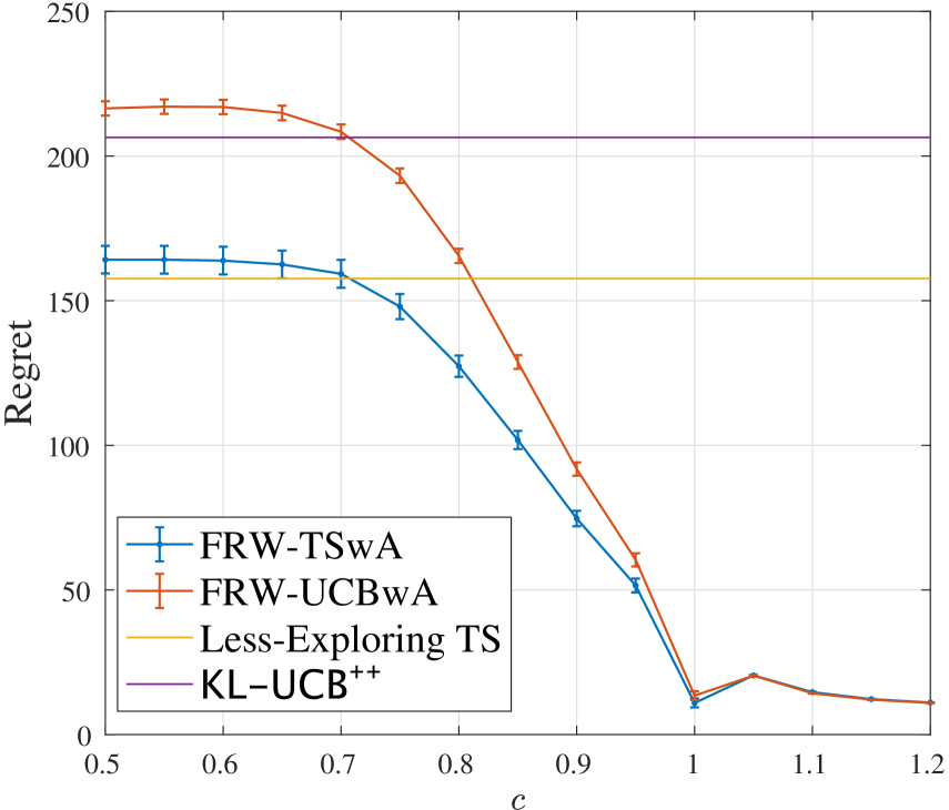
In this section, we conduct numerical experiments to empirically validate our theoretical insights. Due to space limitations, we report our results only for the fixed-regret setting here. Results pertaining to the fixed-reward setting are available in Appendix E, where two particular realizations of our algorithm FRW-ALGwA (as outlined in Algorithm 2) are considered. In each experiment, the reported cumulative regrets are averaged over 2,00020002,000 independent trials and the corresponding standard deviations are displayed as error bars in the figures.
Refer to caption
(a) Instance μsuperscript𝜇\mu^{\dagger}
Refer to caption
(b) Instance μsuperscript𝜇\mu^{\ddagger}
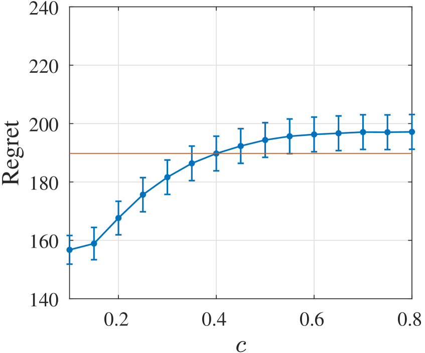
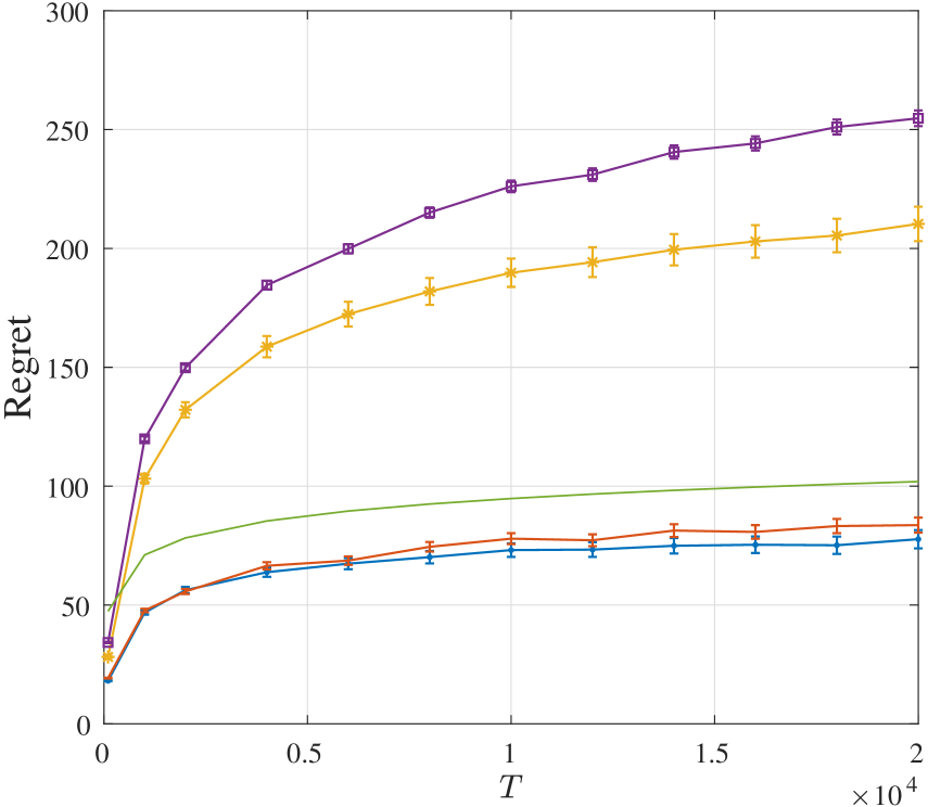
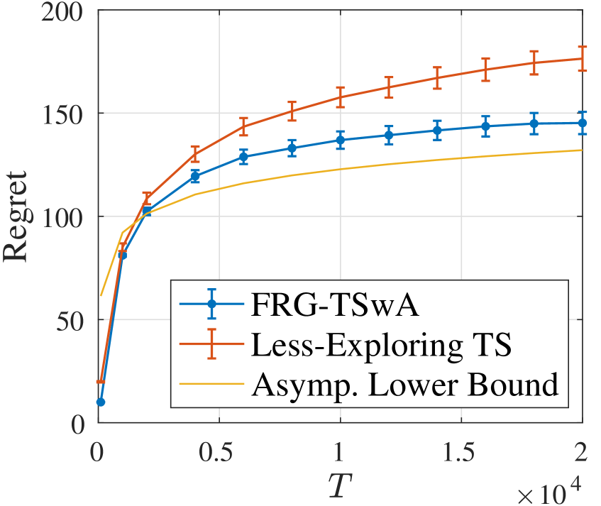
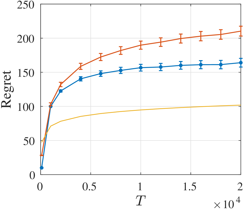
Figure 2: Empirical regrets with abstention regret c=0.1𝑐0.1c=0.1 for different time horizons T𝑇T.

To confirm the benefits of incorporating the abstention option, we compare the performance of our proposed algorithm FRG-TSwA (Algorithm 1) with that of Less-Exploring Thompson Sampling (Jin et al., 2023), which serves as a baseline algorithm without the abstention option. We consider two synthetic bandit instances. The first instance μsuperscript𝜇\mu^{\dagger} with K=7𝐾7K=7 has uniform suboptimality gaps: μ1=1subscriptsuperscript𝜇11\mu^{\dagger}_{1}=1 and μi=0.7subscriptsuperscript𝜇𝑖0.7\mu^{\dagger}_{i}=0.7 for all i[K]{1}𝑖delimited-[]𝐾1i\in[K]\setminus\{1\}. For the second instance μsuperscript𝜇\mu^{\ddagger} with K=10𝐾10K=10, the suboptimality gaps are more diverse: μ1=1subscriptsuperscript𝜇11\mu^{\ddagger}_{1}=1, μi=0.7subscriptsuperscript𝜇𝑖0.7\mu^{\ddagger}_{i}=0.7 for i{2,3,4}𝑖234i\in\{2,3,4\}, μi=0.5subscriptsuperscript𝜇𝑖0.5\mu^{\ddagger}_{i}=0.5 for i{5,6,7}𝑖567i\in\{5,6,7\} and μi=0.3subscriptsuperscript𝜇𝑖0.3\mu^{\ddagger}_{i}=0.3 for i{8,9,10}𝑖8910i\in\{8,9,10\}. The empirical averaged cumulative regrets of both methods with abstention regret c=0.1𝑐0.1c=0.1 for different time horizons T𝑇T are presented in Figure 2. To demonstrate their asymptotic behavior, we also plot the instance-dependent asymptotic lower bound on the cumulative regret (refer to Theorem 3.5) in each sub-figure. It can be observed that FRG-TSwA is clearly superior compared to the non-abstaining baseline, especially for large values of T𝑇T. This demonstrates the advantage of the abstention mechanism. With regard to the growth trend, as the time horizon T𝑇T increases, the curve corresponding to FRG-TSwA closely approximates that of the asymptotic lower bound. This suggests that the expected cumulative regret of FRG-TSwA matches the lower bound asymptotically, thereby substantiating the theoretical results presented in Section 3.
Refer to caption
(a) Instance μsuperscript𝜇\mu^{\dagger}
Refer to caption
(b) Instance μsuperscript𝜇\mu^{\ddagger}
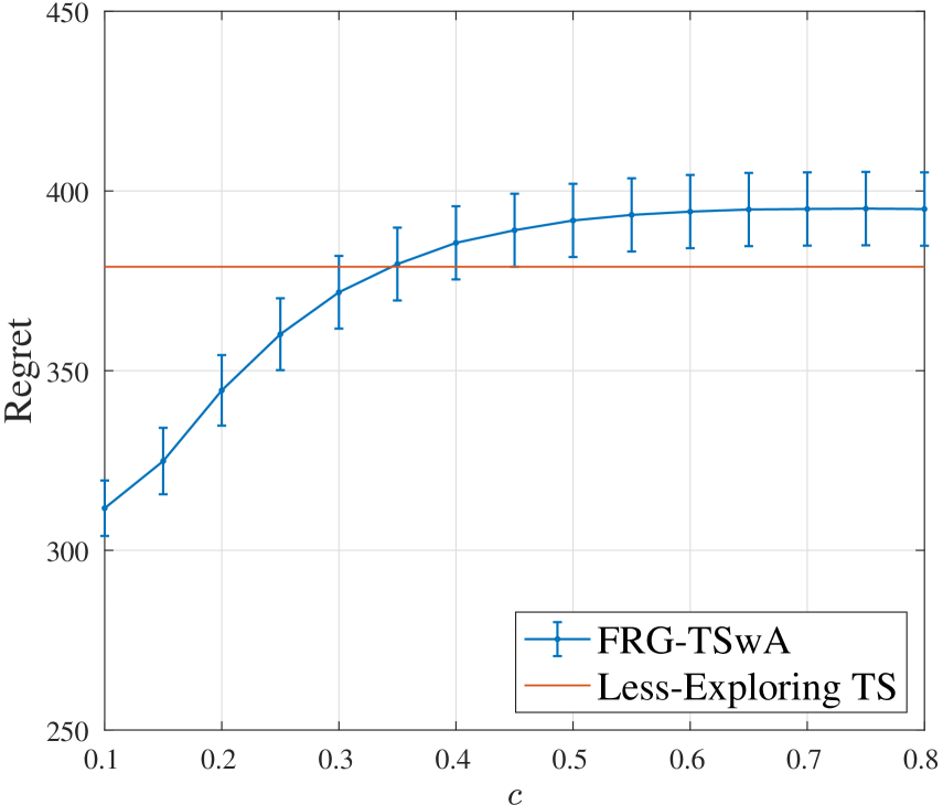
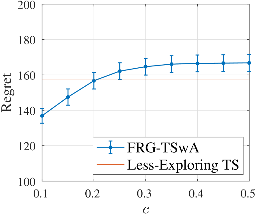
Figure 3: Empirical regrets with time horizon T=10,000𝑇10000T=10,000 for different abstention regrets c𝑐c.

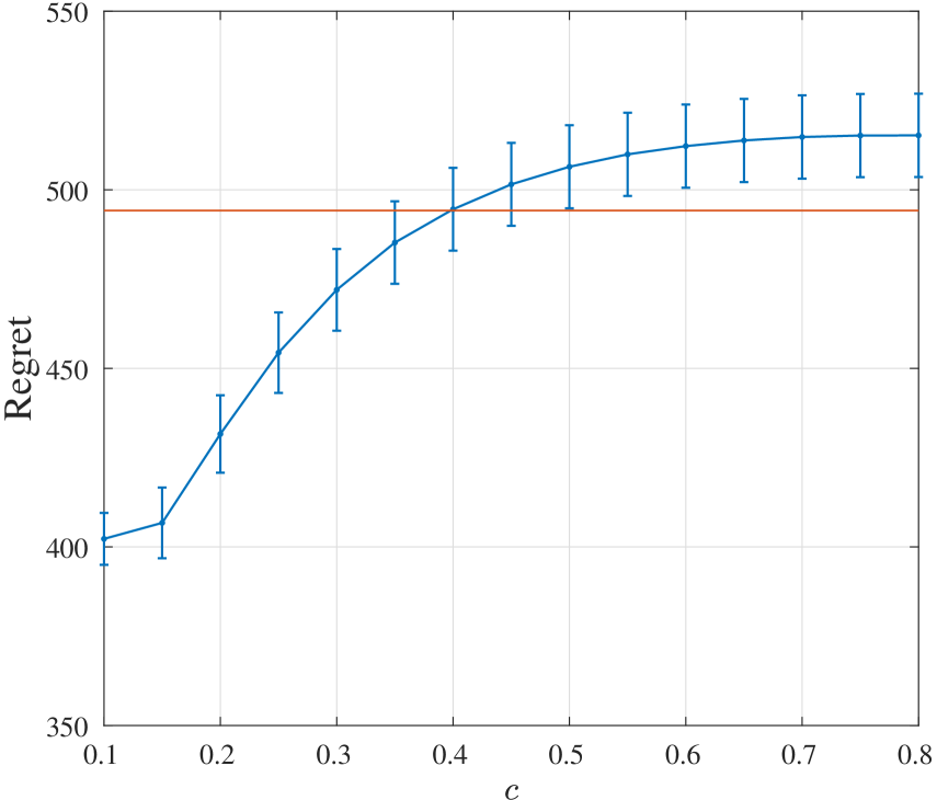
To illustrate the effect of the abstention regret c𝑐c, we evaluate the performance of FRG-TSwA for varying values of c𝑐c, while keeping the time horizon T𝑇T fixed at 10,0001000010,000. The experimental results for both bandit instances μsuperscript𝜇\mu^{\dagger} and μsuperscript𝜇\mu^{\ddagger} are presented in Figure 3. Within each sub-figure, we observe that as c𝑐c increases, the empirical averaged cumulative regret initially increases but eventually saturates beyond a certain threshold value of c𝑐c. These empirical observations align well with our expectations. Indeed, when provided with complete information about the bandit instance, if the abstention regret c𝑐c exceeds the largest suboptimality gap, the agent gains no advantage in choosing the abstention option when selecting any arm. However, we remark that the agent lacks this oracle-like knowledge of the suboptimality gaps and must estimate them on the fly. Consequently, this results in the inevitable selection of the abstention option, even when the abstention regret c𝑐c is large.

6 Conclusions and Future Work

In this paper, we consider, for the first time, a multi-armed bandit model that allows for the possibility of abstaining from accepting the stochastic rewards, alongside the conventional arm selection. This innovative framework is motivated by real-world scenarios where decision-makers may wish to hedge against highly uncertain or risky actions, as exemplified in clinical trials. Within this enriched paradigm, we address both the fixed-regret and fixed-reward settings, providing tight upper and lower bounds on asymptotic and minimax regrets for each scenario. For the fixed-regret setting, we thoughtfully adapt a recently developed asymptotically and minimax optimal algorithm by Jin et al. (2023) to accommodate the abstention option while preserving its attractive optimality characteristics. For the fixed-reward setting, we convert any asymptotically and minimax optimal algorithm for the canonical model into one that retains these optimality properties when the abstention option is present. Finally, experiments on synthetic datasets validate our theoretical results and clearly demonstrate the advantage of incorporating the abstention option.

As highlighted in Remark 3.6, a fruitful avenue for future research lies in expanding the abstention model from K𝐾K-armed bandits to linear bandits. An intriguing inquiry is whether the inclusion of the abstention feature can lead to enhanced asymptotic and minimax theoretical guarantees. Furthermore, in our work, the abstention option exerts no influence on the stochastic observation from the selected arm. Delving into more sophisticated and general approaches to model the effect of the abstention option promises as a captivating future direction.

References

  • Agrawal & Goyal (2012) Agrawal, S. and Goyal, N. Analysis of Thompson sampling for the multi-armed bandit problem. In Conference on Learning Theory (COLT), pp.  39–1. JMLR Workshop and Conference Proceedings, 2012.
  • Agrawal & Goyal (2017) Agrawal, S. and Goyal, N. Near-optimal regret bounds for Thompson sampling. Journal of the ACM (JACM), 64(5):1–24, 2017.
  • Audibert & Bubeck (2009) Audibert, J.-Y. and Bubeck, S. Minimax policies for adversarial and stochastic bandits. In Conference on Learning Theory (COLT), volume 7, pp.  1–122, 2009.
  • Auer et al. (1995) Auer, P., Cesa-Bianchi, N., Freund, Y., and Schapire, R. E. Gambling in a rigged casino: The adversarial multi-armed bandit problem. In Proceedings of IEEE 36th annual foundations of computer science, pp.  322–331. IEEE, 1995.
  • Auer et al. (2002) Auer, P., Cesa-Bianchi, N., and Fischer, P. Finite-time analysis of the multiarmed bandit problem. Machine Learning, 47(2):235–256, 2002.
  • Bartlett & Wegkamp (2008) Bartlett, P. L. and Wegkamp, M. H. Classification with a reject option using a hinge loss. Journal of Machine Learning Research, 9(8), 2008.
  • Cappé et al. (2013) Cappé, O., Garivier, A., Maillard, O.-A., Munos, R., and Stoltz, G. Kullback–Leibler upper confidence bounds for optimal sequential allocation. Annals of Statistics, pp.  1516–1541, 2013.
  • Cheng et al. (2010) Cheng, W., Rademaker, M., De Baets, B., and Hüllermeier, E. Predicting partial orders: Ranking with abstention. In Machine Learning and Knowledge Discovery in Databases: European Conference, ECML PKDD 2010, pp.  215–230. Springer, 2010.
  • Chow (1957) Chow, C.-K. An optimum character recognition system using decision functions. IRE Transactions on Electronic Computers, pp.  247–254, 1957.
  • Chow (1970) Chow, C.-K. On optimum recognition error and reject tradeoff. IEEE Transactions on Information Theory, 16(1):41–46, 1970.
  • Cortes et al. (2016) Cortes, C., DeSalvo, G., and Mohri, M. Learning with rejection. In Algorithmic Learning Theory: 27th International Conference, ALT 2016, Bari, Italy, October 19-21, 2016, Proceedings 27, pp.  67–82. Springer, 2016.
  • Cortes et al. (2018) Cortes, C., DeSalvo, G., Gentile, C., Mohri, M., and Yang, S. Online learning with abstention. In International Conference on Machine Learning, pp.  1059–1067. PMLR, 2018.
  • Garivier et al. (2019) Garivier, A., Ménard, P., and Stoltz, G. Explore first, exploit next: The true shape of regret in bandit problems. Mathematics of Operations Research, 44(2):377–399, 2019.
  • Herbei & Wegkamp (2006) Herbei, R. and Wegkamp, M. H. Classification with reject option. The Canadian Journal of Statistics / La Revue Canadienne de Statistique, pp.  709–721, 2006.
  • Honda & Takemura (2010) Honda, J. and Takemura, A. An asymptotically optimal bandit algorithm for bounded support models. In Conference on Learning Theory, pp.  67–79. Citeseer, 2010.
  • Jin et al. (2021) Jin, T., Xu, P., Shi, J., Xiao, X., and Gu, Q. Mots: Minimax optimal thompson sampling. In International Conference on Machine Learning, pp.  5074–5083. PMLR, 2021.
  • Jin et al. (2023) Jin, T., Yang, X., Xiao, X., and Xu, P. Thompson sampling with less exploration is fast and optimal. In Proceedings of the 40th International Conference on Machine Learning, volume 202, pp.  15239–15261. PMLR, 2023.
  • Kalai & Kanade (2021) Kalai, A. and Kanade, V. Towards optimally abstaining from prediction with ood test examples. Advances in Neural Information Processing Systems, 34:12774–12785, 2021.
  • Kaufmann et al. (2012) Kaufmann, E., Korda, N., and Munos, R. Thompson sampling: An asymptotically optimal finite-time analysis. In Algorithmic Learning Theory: 23rd International Conference, ALT 2012, Lyon, France, October 29-31, 2012. Proceedings 23, pp.  199–213. Springer, 2012.
  • Korda et al. (2013) Korda, N., Kaufmann, E., and Munos, R. Thompson sampling for 1-dimensional exponential family bandits. Advances in Neural Information Processing Systems, 26, 2013.
  • Lai & Robbins (1985) Lai, T. L. and Robbins, H. Asymptotically efficient adaptive allocation rules. Advances in Applied Mathematics, 6(1):4–22, 1985.
  • Lattimore (2018) Lattimore, T. Refining the confidence level for optimistic bandit strategies. Journal of Machine Learning Research, 19(1):765–796, 2018.
  • Lattimore & Szepesvári (2017) Lattimore, T. and Szepesvári, C. The end of optimism? An asymptotic analysis of finite-armed linear bandits. In Artificial Intelligence and Statistics, pp.  728–737. PMLR, 2017.
  • Lattimore & Szepesvári (2020) Lattimore, T. and Szepesvári, C. Bandit Algorithms. Cambridge University Press, 2020.
  • Littlestone & Warmuth (1994) Littlestone, N. and Warmuth, M. K. The weighted majority algorithm. Information and Computation, 108(2):212–261, 1994.
  • Mao et al. (2023) Mao, A., Mohri, M., and Zhong, Y. Ranking with abstention. arXiv preprint arXiv:2307.02035, 2023.
  • Ménard & Garivier (2017) Ménard, P. and Garivier, A. A minimax and asymptotically optimal algorithm for stochastic bandits. In International Conference on Algorithmic Learning Theory, pp.  223–237. PMLR, 2017.
  • Neu & Zhivotovskiy (2020) Neu, G. and Zhivotovskiy, N. Fast rates for online prediction with abstention. In Conference on Learning Theory, pp.  3030–3048. PMLR, 2020.
  • Thompson (1933) Thompson, W. R. On the likelihood that one unknown probability exceeds another in view of the evidence of two samples. Biometrika, 25(3-4):285–294, 1933.
  • Tsybakov (2009) Tsybakov, A. B. Introduction to Nonparametric Estimation. Springer Series in Statistics. Springer, 2009.
  • Wiener & El-Yaniv (2012) Wiener, Y. and El-Yaniv, R. Pointwise tracking the optimal regression function. Advances in Neural Information Processing Systems, 25, 2012.
  • Zaoui et al. (2020) Zaoui, A., Denis, C., and Hebiri, M. Regression with reject option and application to knn. Advances in Neural Information Processing Systems, 33:20073–20082, 2020.

Appendix A Asymptotic and Minimax Optimality in Canonical Multi-Armed Bandits

In the canonical multi-armed bandit model, there is no additional abstention option. Given a bandit instance μ𝒰𝜇𝒰\mu\in\mathcal{U}, at each time step t𝑡t\in\mathbb{N}, the agent employs an online algorithm π𝜋\pi to choose an arm Atsubscript𝐴𝑡A_{t} from the arm set [K]delimited-[]𝐾[K], and then observes a random variable Xtsubscript𝑋𝑡X_{t} from the selected arm Atsubscript𝐴𝑡A_{t}, which is drawn from a Gaussian distribution 𝒩(μAt,1)𝒩subscript𝜇subscript𝐴𝑡1\mathcal{N}(\mu_{A_{t}},1) and independent of observations from previous time steps. The choice of Atsubscript𝐴𝑡A_{t} might depend on the prior decisions and observations. To describe the setup formally, Atsubscript𝐴𝑡A_{t} is t1CAsubscriptsuperscriptCA𝑡1\mathcal{F}^{\mathrm{CA}}_{t-1}-measurable, where tCA:=σ(A1,X1,A2,X2,,At,Xt)assignsubscriptsuperscriptCA𝑡𝜎subscript𝐴1subscript𝑋1subscript𝐴2subscript𝑋2subscript𝐴𝑡subscript𝑋𝑡\mathcal{F}^{\mathrm{CA}}_{t}:=\sigma(A_{1},X_{1},A_{2},X_{2},\ldots,A_{t},X_{t}) represents the σ𝜎\sigma-field generated by the cumulative interaction history up to and including time t𝑡t. Subsequently, the agent suffers an instantaneous regret of μ1Xtsubscript𝜇1subscript𝑋𝑡\mu_{1}-X_{t}.

The agent aims at minimizing the expected cumulative regret over a time horizon T𝑇T, which is defined as

RμCA(T,π)=Tμ1𝔼[t=1TXt].subscriptsuperscript𝑅CA𝜇𝑇𝜋𝑇subscript𝜇1𝔼delimited-[]superscriptsubscript𝑡1𝑇subscript𝑋𝑡R^{\mathrm{CA}}_{\mu}(T,\pi)=T\mu_{1}-\mathbb{E}\left[\sum_{t=1}^{T}X_{t}\right].

We refer to the collection of all online policies for the canonical multi-armed bandit model as ΠCAsuperscriptΠCA\Pi^{\mathrm{CA}}.

Remark A.1.

It is worth noting that any algorithm designed for canonical multi-armed bandit model possesses the capability to decide the arm Atsubscript𝐴𝑡A_{t} to pull at each time step t𝑡t, based on the partial interaction history (A1,X1,A2,X2,,At1,Xt1)subscript𝐴1subscript𝑋1subscript𝐴2subscript𝑋2subscript𝐴𝑡1subscript𝑋𝑡1(A_{1},X_{1},A_{2},X_{2},\ldots,A_{t-1},X_{t-1}), within the abstention model. Conversely, any algorithm tailored for the abstention model in the fixed-regret setting (or in the fixed-reward setting) can be applied to the canonical multi-armed bandit model, provided that the abstention regret (or the abstention reward) has been predetermined. Specifically, the algorithm can determine both the selected arm Atsubscript𝐴𝑡A_{t} and the binary abstention variable Btsubscript𝐵𝑡B_{t}, although Btsubscript𝐵𝑡B_{t} is purely auxiliary and exerts no influence on the cumulative regret RμCA(T,π)subscriptsuperscript𝑅CA𝜇𝑇𝜋R^{\mathrm{CA}}_{\mu}(T,\pi).

Lower bounds.

Both the asymptotic and minimax lower bounds for the canonical multi-armed bandit model have been thoroughly established (Lai & Robbins, 1985; Auer et al., 1995). For a comprehensive overview, refer to Sections 15 and 16 of Lattimore & Szepesvári (2020). Here, we summarize the results in the following:

Definition A.2 (RCAsuperscript𝑅CAR^{\mathrm{CA}}-consistency).

An algorithm πΠCA𝜋superscriptΠCA\pi\in\Pi^{\mathrm{CA}} is said to be RCAsuperscript𝑅CAR^{\mathrm{CA}}-consistent if for all bandit instances μ𝒰𝜇𝒰\mu\in\mathcal{U} and a>0𝑎0a>0, RμCA(T,π)=o(Ta)subscriptsuperscript𝑅CA𝜇𝑇𝜋𝑜superscript𝑇𝑎R^{\mathrm{CA}}_{\mu}(T,\pi)=o(T^{a}).

Theorem A.3.

For any bandit instance μ𝒰𝜇𝒰\mu\in\mathcal{U} and RCAsuperscript𝑅CAR^{\mathrm{CA}}-consistent algorithm π𝜋\pi, it holds that

lim infTRμCA(T,π)logTi>12Δi.subscriptlimit-infimum𝑇subscriptsuperscript𝑅CA𝜇𝑇𝜋𝑇subscript𝑖12subscriptΔ𝑖\liminf_{T\to\infty}\frac{R^{\mathrm{CA}}_{\mu}(T,\pi)}{\log T}\geq\sum_{i>1}\frac{2}{\Delta_{i}}.

For any time horizon TK𝑇𝐾T\geq K, there exists a universal constant α>0𝛼0\alpha>0 such that

infπΠCAsupμ𝒰RμCA(T,π)αKT.subscriptinfimum𝜋superscriptΠCAsubscriptsupremum𝜇𝒰subscriptsuperscript𝑅CA𝜇𝑇𝜋𝛼𝐾𝑇\inf_{\pi\in\Pi^{\mathrm{CA}}}\sup_{\mu\in\mathcal{U}}{R^{\mathrm{CA}}_{\mu}(T,\pi)}\geq\alpha\sqrt{KT}.

Asymptotic and minimax optimality.

According to Theorem A.3, in the canonical bandit model, an algorithm πΠCA𝜋superscriptΠCA\pi\in\Pi^{\mathrm{CA}} is said to be asymptotically optimal if for all bandit instances μ𝒰𝜇𝒰\mu\in\mathcal{U}, it ensures that

limTRμCA(T,π)logT=i>12Δi.subscript𝑇subscriptsuperscript𝑅CA𝜇𝑇𝜋𝑇subscript𝑖12subscriptΔ𝑖\lim_{T\to\infty}\frac{R^{\mathrm{CA}}_{\mu}(T,\pi)}{\log T}=\sum_{i>1}\frac{2}{\Delta_{i}}.

Furthermore, it is said to be minimax optimal if there exists a universal constant α>0𝛼0\alpha>0 such that

RμCA(T,π)α(KT+i>1Δi).subscriptsuperscript𝑅CA𝜇𝑇𝜋𝛼𝐾𝑇subscript𝑖1subscriptΔ𝑖{R^{\mathrm{CA}}_{\mu}(T,\pi)}\leq\alpha\left(\sqrt{KT}+\sum_{i>1}\Delta_{i}\right).

To the best of our knowledge, for canonical multi-armed bandits with Gaussian rewards, KL-UCB++superscriptKL-UCBabsent\text{KL-UCB}^{++} (Ménard & Garivier, 2017), ADA-UCB (Lattimore, 2018), MOTS-𝒥𝒥\mathcal{J} (Jin et al., 2021) and Less-Exploring Thompson Sampling (Jin et al., 2023) exhibit simultaneous asymptotic and minimax optimality. As their names suggest, the former two algorithms follow the UCB-style, while the latter two are rooted in Thompson Sampling.

Remark A.4.

One valuable byproduct derived from the proof of the asymptotic lower bound in Theorem A.3 is that, for any RCAsuperscript𝑅CAR^{\mathrm{CA}}-consistent algorithm π𝜋\pi, bandit instance μ𝒰𝜇𝒰\mu\in\mathcal{U} and suboptimal arm i>1𝑖1i>1, we have

lim infT𝔼[Ni(T)]logT2Δi2.subscriptlimit-infimum𝑇𝔼subscript𝑁𝑖𝑇𝑇2superscriptsubscriptΔ𝑖2\liminf_{T\rightarrow\infty}\frac{\operatorname{\mathbb{E}}[N_{i}(T)]}{\log T}\geq\frac{2}{\Delta_{i}^{2}}.

Therefore, any algorithm that is asymptotically optimal ensures that for all suboptimal arms i>1𝑖1i>1,

limT𝔼[Ni(T)]logT=2Δi2.subscript𝑇𝔼subscript𝑁𝑖𝑇𝑇2superscriptsubscriptΔ𝑖2\lim_{T\rightarrow\infty}\frac{\operatorname{\mathbb{E}}[N_{i}(T)]}{\log T}=\frac{2}{\Delta_{i}^{2}}.

Appendix B Auxiliary Lemmas

Lemma B.1 (Bretagnolle–Huber inequality (Tsybakov, 2009)).

Let \mathbb{P} and superscript\mathbb{P}^{\prime} be two probability distributions on the same measurable space (Ω,)Ω(\Omega,\mathcal{F}). For any event A𝐴A\in\mathcal{F} and its complement Ac=ΩAsuperscript𝐴𝑐Ω𝐴A^{c}=\Omega\setminus A, the following inequality holds:

(A)+(Ac)12exp(KL(,)),𝐴superscriptsuperscript𝐴𝑐12KLsuperscript\mathbb{P}(A)+\mathbb{P}^{\prime}(A^{c})\geq\frac{1}{2}\exp(-\mathrm{KL}(\mathbb{P},\mathbb{P}^{\prime})),

where KL(,)KLsuperscript\mathrm{KL}(\mathbb{P},\mathbb{P}^{\prime}) denotes the Kullback–Leibler (KL) divergence between \mathbb{P} and superscript\mathbb{P}^{\prime}.

Lemma B.2 (Divergence decomposition lemma).

Consider both the fixed-regret setting and the fixed-reward setting. Fix an arbitrary policy π𝜋\pi. Let ν=(1,,K)𝜈subscript1subscript𝐾\nu=(\mathbb{P}_{1},\ldots,\mathbb{P}_{K}) represent the reward distributions associated with one bandit instance, and let ν=(1,,K)superscript𝜈superscriptsubscript1superscriptsubscript𝐾\nu^{\prime}=(\mathbb{P}_{1}^{\prime},\ldots,\mathbb{P}_{K}^{\prime}) represent the reward distributions associated with another bandit instance. Define ν,csubscript𝜈𝑐\mathbb{P}_{\nu,c} as the probability distribution of the sequence (A1,B1,X1,,AT,BT,XT)subscript𝐴1subscript𝐵1subscript𝑋1subscript𝐴𝑇subscript𝐵𝑇subscript𝑋𝑇(A_{1},B_{1},X_{1},\ldots,A_{T},B_{T},X_{T}) induced by the algorithm π𝜋\pi under the abstention regret c𝑐c in the fixed-regret setting (or the abstention reward c𝑐c in the fixed-reward setting) for the bandit instance ν𝜈\nu. Similarly, let ν,csubscriptsuperscript𝜈𝑐\mathbb{P}_{\nu^{\prime},c} denote the same for the bandit instance νsuperscript𝜈\nu^{\prime}. Then the KL divergence between ν,csubscript𝜈𝑐\mathbb{P}_{\nu,c} and ν,csubscriptsuperscript𝜈𝑐\mathbb{P}_{\nu^{\prime},c} can be decomposed as:

KL(ν,c,ν,c)=i[K]𝔼ν,c[Ni(T)]KL(i,i).KLsubscript𝜈𝑐subscriptsuperscript𝜈𝑐subscript𝑖delimited-[]𝐾subscript𝔼𝜈𝑐subscript𝑁𝑖𝑇KLsubscript𝑖superscriptsubscript𝑖\mathrm{KL}\left(\mathbb{P}_{\nu,c},\mathbb{P}_{\nu^{\prime},c}\right)=\sum_{i\in[K]}\operatorname{\mathbb{E}}_{\nu,c}[N_{i}(T)]\mathrm{KL}\left(\mathbb{P}_{i},\mathbb{P}_{i}^{\prime}\right).

The proof of Lemma B.2 is similar to the well-known proof of divergence decomposition in the canonical multi-armed bandit model (excluding abstention), and is therefore omitted. This proof can be located, for instance, in Garivier et al. (2019, Section 2.1) and Lattimore & Szepesvári (2020, Lemma 15.1).

Lemma B.3 (Hoeffding’s inequality for sub-Gaussian random variables).

Let X1,,Xnsubscript𝑋1subscript𝑋𝑛X_{1},\ldots,X_{n} be independent σ𝜎\sigma-sub-Gaussian random variables with mean μ𝜇\mu. Then for any ε0𝜀0\varepsilon\geq 0,

(μ^μ+ε)exp(nε22σ2) and (μ^με)exp(nε22σ2)formulae-sequence^𝜇𝜇𝜀𝑛superscript𝜀22superscript𝜎2 and ^𝜇𝜇𝜀𝑛superscript𝜀22superscript𝜎2\mathbb{P}(\hat{\mu}\geq\mu+\varepsilon)\leq\exp\left(-\frac{n\varepsilon^{2}}{2\sigma^{2}}\right)\quad\text{ and }\quad\mathbb{P}(\hat{\mu}\leq\mu-\varepsilon)\leq\exp\left(-\frac{n\varepsilon^{2}}{2\sigma^{2}}\right)

where μ^:=1ni=1nXiassign^𝜇1𝑛superscriptsubscript𝑖1𝑛subscript𝑋𝑖\hat{\mu}:=\frac{1}{n}\sum_{i=1}^{n}X_{i}.

Lemma B.4.

Let {Xi}isubscriptsubscript𝑋𝑖𝑖\{X_{i}\}_{i\in\mathbb{N}} be a sequence of independent σ𝜎\sigma-sub-Gaussian random variables with mean μ𝜇\mu. Then for any ε>0𝜀0\varepsilon>0 and N𝑁N\in\mathbb{N},

n=1N(μ^nμ+ε)2σ2ε2 and n=1N(μ^nμε)2σ2ε2formulae-sequencesuperscriptsubscript𝑛1𝑁subscript^𝜇𝑛𝜇𝜀2superscript𝜎2superscript𝜀2 and superscriptsubscript𝑛1𝑁subscript^𝜇𝑛𝜇𝜀2superscript𝜎2superscript𝜀2\sum_{n=1}^{N}\mathbb{P}(\hat{\mu}_{n}\geq\mu+\varepsilon)\leq\frac{2\sigma^{2}}{\varepsilon^{2}}\quad\text{ and }\quad\sum_{n=1}^{N}\mathbb{P}(\hat{\mu}_{n}\leq\mu-\varepsilon)\leq\frac{2\sigma^{2}}{\varepsilon^{2}}

where μ^n:=1ni=1nXiassignsubscript^𝜇𝑛1𝑛superscriptsubscript𝑖1𝑛subscript𝑋𝑖\hat{\mu}_{n}:=\frac{1}{n}\sum_{i=1}^{n}X_{i}.

Proof of Lemma B.4.

By symmetry, it suffices to prove the first part. According to Lemma B.3, we have

n=1N(μ^nμ+ε)superscriptsubscript𝑛1𝑁subscript^𝜇𝑛𝜇𝜀\displaystyle\sum_{n=1}^{N}\mathbb{P}(\hat{\mu}_{n}\geq\mu+\varepsilon) n=1Nexp(nε22σ2)absentsuperscriptsubscript𝑛1𝑁𝑛superscript𝜀22superscript𝜎2\displaystyle\leq\sum_{n=1}^{N}\exp\left(-\frac{n\varepsilon^{2}}{2\sigma^{2}}\right)
exp(ε22σ2)1exp(ε22σ2)absentsuperscript𝜀22superscript𝜎21superscript𝜀22superscript𝜎2\displaystyle\leq\frac{\exp\left(-\frac{\varepsilon^{2}}{2\sigma^{2}}\right)}{1-\exp\left(-\frac{\varepsilon^{2}}{2\sigma^{2}}\right)}
=1exp(ε22σ2)1absent1superscript𝜀22superscript𝜎21\displaystyle=\frac{1}{\exp\left(\frac{\varepsilon^{2}}{2\sigma^{2}}\right)-1}
2σ2ε2absent2superscript𝜎2superscript𝜀2\displaystyle\leq\frac{2\sigma^{2}}{\varepsilon^{2}}

where the last inequality follows from the fact that ex1xsuperscript𝑒𝑥1𝑥e^{x}-1\geq x for any x0𝑥0x\geq 0. ∎

Appendix C Analysis of the Fixed-Regret Setting

C.1 Upper Bounds

Proof of Theorem 3.3.

Due to the law of total expectation, we can decompose the regret Rμ,cRG(T,π)subscriptsuperscript𝑅RG𝜇𝑐𝑇𝜋R^{\mathrm{RG}}_{\mu,c}(T,\pi) as

Rμ,cRG(T,π)subscriptsuperscript𝑅RG𝜇𝑐𝑇𝜋\displaystyle R^{\mathrm{RG}}_{\mu,c}(T,\pi) =𝔼[t=1T((μ1Xt)𝟙{Bt=0}+c𝟙{Bt=1})]absent𝔼delimited-[]superscriptsubscript𝑡1𝑇subscript𝜇1subscript𝑋𝑡1subscript𝐵𝑡0𝑐1subscript𝐵𝑡1\displaystyle=\mathbb{E}\left[\sum_{t=1}^{T}\big{(}(\mu_{1}-X_{t})\cdot\mathbbm{1}\{B_{t}=0\}+c\cdot\mathbbm{1}\{B_{t}=1\}\big{)}\right]
=𝔼[t=1T((μ1μAt)𝟙{Bt=0}+c𝟙{Bt=1})]absent𝔼delimited-[]superscriptsubscript𝑡1𝑇subscript𝜇1subscript𝜇subscript𝐴𝑡1subscript𝐵𝑡0𝑐1subscript𝐵𝑡1\displaystyle=\mathbb{E}\left[\sum_{t=1}^{T}\big{(}(\mu_{1}-\mu_{A_{t}})\cdot\mathbbm{1}\{B_{t}=0\}+c\cdot\mathbbm{1}\{B_{t}=1\}\big{)}\right]
=c𝔼[N1(1)(T)]+i>1(Δi𝔼[Ni(0)(T)]+c𝔼[Ni(1)(T)]).absent𝑐𝔼superscriptsubscript𝑁11𝑇subscript𝑖1subscriptΔ𝑖𝔼superscriptsubscript𝑁𝑖0𝑇𝑐𝔼superscriptsubscript𝑁𝑖1𝑇\displaystyle=c\cdot\operatorname{\mathbb{E}}[N_{1}^{(1)}(T)]+\sum_{i>1}\left(\Delta_{i}\cdot\operatorname{\mathbb{E}}[N_{i}^{(0)}(T)]+c\cdot\operatorname{\mathbb{E}}[N_{i}^{(1)}(T)]\right). (4)

For any arm i𝑖i with Δi<csubscriptΔ𝑖𝑐\Delta_{i}<c (including the best arm), it holds that

𝔼[Ni(1)(T)]𝔼superscriptsubscript𝑁𝑖1𝑇\displaystyle\phantom{\ =\ }\operatorname{\mathbb{E}}[N_{i}^{(1)}(T)]
=𝔼[t=1T𝕀{At=i and Bt=1}]absent𝔼superscriptsubscript𝑡1𝑇𝕀subscript𝐴𝑡𝑖 and subscript𝐵𝑡1\displaystyle=\operatorname{\mathbb{E}}\left[\sum_{t=1}^{T}\mathbb{I}\left\{A_{t}=i\text{ and }B_{t}=1\right\}\right]
𝔼[t=1T𝕀{At=i and Ktc}]absent𝔼superscriptsubscript𝑡1𝑇𝕀subscript𝐴𝑡𝑖 and 𝐾𝑡𝑐\displaystyle\leq\operatorname{\mathbb{E}}\left[\sum_{t=1}^{T}\mathbb{I}\left\{A_{t}=i\text{ and }\sqrt{\frac{K}{t}}\geq c\right\}\right]
+𝔼[t=K+1T𝕀{At=i and maxj[K]{i}(μ^j(t1)6logt+2log(c1)Nj(t1))μ^i(t1)c}]𝔼superscriptsubscript𝑡𝐾1𝑇𝕀subscript𝐴𝑡𝑖 and subscript𝑗delimited-[]𝐾𝑖subscript^𝜇𝑗𝑡16𝑡2𝑐1subscript𝑁𝑗𝑡1subscript^𝜇𝑖𝑡1𝑐\displaystyle\phantom{\ =\ }+\operatorname{\mathbb{E}}\left[\sum_{t=K+1}^{T}\mathbb{I}\left\{A_{t}=i\text{ and }\max_{j\in[K]\setminus\{i\}}\left(\hat{\mu}_{j}(t-1)-\sqrt{\frac{6\log t+2\log(c\vee 1)}{N_{j}(t-1)}}\right)-\hat{\mu}_{i}(t-1)\geq c\right\}\right]
𝔼[t=1T𝕀{At=i and Ktc}]absent𝔼superscriptsubscript𝑡1𝑇𝕀subscript𝐴𝑡𝑖 and 𝐾𝑡𝑐\displaystyle\leq\operatorname{\mathbb{E}}\left[\sum_{t=1}^{T}\mathbb{I}\left\{A_{t}=i\text{ and }\sqrt{\frac{K}{t}}\geq c\right\}\right]
+𝔼[t=K+1T𝕀{At=i and maxj[K](μ^j(t1)6logt+2log(c1)Nj(t1))μ1}]𝔼superscriptsubscript𝑡𝐾1𝑇𝕀subscript𝐴𝑡𝑖 and subscript𝑗delimited-[]𝐾subscript^𝜇𝑗𝑡16𝑡2𝑐1subscript𝑁𝑗𝑡1subscript𝜇1\displaystyle\phantom{\ =\ }+\operatorname{\mathbb{E}}\left[\sum_{t=K+1}^{T}\mathbb{I}\left\{A_{t}=i\text{ and }\max_{j\in[K]}\left(\hat{\mu}_{j}(t-1)-\sqrt{\frac{6\log t+2\log(c\vee 1)}{N_{j}(t-1)}}\right)\geq\mu_{1}\right\}\right]
+𝔼[t=K+1T𝕀{At=i and μ1μ^i(t1)c}]𝔼superscriptsubscript𝑡𝐾1𝑇𝕀subscript𝐴𝑡𝑖 and subscript𝜇1subscript^𝜇𝑖𝑡1𝑐\displaystyle\phantom{\ =\ }+\operatorname{\mathbb{E}}\left[\sum_{t=K+1}^{T}\mathbb{I}\left\{A_{t}=i\text{ and }\mu_{1}-\hat{\mu}_{i}(t-1)\geq c\right\}\right] (5)

where the last inequality arises from the observation that when At=isubscript𝐴𝑡𝑖A_{t}=i,

{maxj[K]{i}(μ^j(t1)6logt+2log(c1)Nj(t1))μ^i(t1)c}subscript𝑗delimited-[]𝐾𝑖subscript^𝜇𝑗𝑡16𝑡2𝑐1subscript𝑁𝑗𝑡1subscript^𝜇𝑖𝑡1𝑐\displaystyle\phantom{\ =\ }\left\{\max_{j\in[K]\setminus\{i\}}\left(\hat{\mu}_{j}(t-1)-\sqrt{\frac{6\log t+2\log(c\vee 1)}{N_{j}(t-1)}}\right)-\hat{\mu}_{i}(t-1)\geq c\right\}
{maxj[K]{i}(μ^j(t1)6logt+2log(c1)Nj(t1))μ1}{μ1μ^i(t1)c}absentsubscript𝑗delimited-[]𝐾𝑖subscript^𝜇𝑗𝑡16𝑡2𝑐1subscript𝑁𝑗𝑡1subscript𝜇1subscript𝜇1subscript^𝜇𝑖𝑡1𝑐\displaystyle\subseteq\left\{\max_{j\in[K]\setminus\{i\}}\left(\hat{\mu}_{j}(t-1)-\sqrt{\frac{6\log t+2\log(c\vee 1)}{N_{j}(t-1)}}\right)\geq\mu_{1}\right\}\cup\left\{\mu_{1}-\hat{\mu}_{i}(t-1)\geq c\right\}
{maxj[K](μ^j(t1)6logt+2log(c1)Nj(t1))μ1}{μ1μ^i(t1)c}.absentsubscript𝑗delimited-[]𝐾subscript^𝜇𝑗𝑡16𝑡2𝑐1subscript𝑁𝑗𝑡1subscript𝜇1subscript𝜇1subscript^𝜇𝑖𝑡1𝑐\displaystyle\subseteq\left\{\max_{j\in[K]}\left(\hat{\mu}_{j}(t-1)-\sqrt{\frac{6\log t+2\log(c\vee 1)}{N_{j}(t-1)}}\right)\geq\mu_{1}\right\}\cup\left\{\mu_{1}-\hat{\mu}_{i}(t-1)\geq c\right\}.

For convenience, for any i[K]𝑖delimited-[]𝐾i\in[K] such that Δi<csubscriptΔ𝑖𝑐\Delta_{i}<c, we introduce three shorthand notations to represent the terms in (5):

{()i:=𝔼[t=1T𝕀{At=i and Ktc}]()i:=𝔼[t=K+1T𝕀{At=i and maxj[K](μ^j(t1)6logt+2log(c1)Nj(t1))μ1}]()i:=𝔼[t=K+1T𝕀{At=i and μ1μ^i(t1)c}].casesassignsubscript𝑖𝔼superscriptsubscript𝑡1𝑇𝕀subscript𝐴𝑡𝑖 and 𝐾𝑡𝑐otherwiseassignsubscript𝑖𝔼superscriptsubscript𝑡𝐾1𝑇𝕀subscript𝐴𝑡𝑖 and subscript𝑗delimited-[]𝐾subscript^𝜇𝑗𝑡16𝑡2𝑐1subscript𝑁𝑗𝑡1subscript𝜇1otherwiseassignsubscript𝑖𝔼superscriptsubscript𝑡𝐾1𝑇𝕀subscript𝐴𝑡𝑖 and subscript𝜇1subscript^𝜇𝑖𝑡1𝑐otherwise\begin{cases}\vspace*{4pt}(\clubsuit)_{i}:=\operatorname{\mathbb{E}}\left[\sum_{t=1}^{T}\mathbb{I}\left\{A_{t}=i\text{ and }\sqrt{\frac{K}{t}}\geq c\right\}\right]\\ \vspace*{4pt}(\spadesuit)_{i}:=\operatorname{\mathbb{E}}\left[\sum_{t=K+1}^{T}\mathbb{I}\left\{A_{t}=i\text{ and }\max_{j\in[K]}\left(\hat{\mu}_{j}(t-1)-\sqrt{\frac{6\log t+2\log(c\vee 1)}{N_{j}(t-1)}}\right)\geq\mu_{1}\right\}\right]\\ (\blacksquare)_{i}:=\operatorname{\mathbb{E}}\left[\sum_{t=K+1}^{T}\mathbb{I}\left\{A_{t}=i\text{ and }\mu_{1}-\hat{\mu}_{i}(t-1)\geq c\right\}\right].\end{cases}

We will deal with ()isubscript𝑖(\clubsuit)_{i} and ()isubscript𝑖(\spadesuit)_{i} later for the two forms of upper bounds.

On the other hand, for the term ()isubscript𝑖(\blacksquare)_{i}, we have

()isubscript𝑖\displaystyle(\blacksquare)_{i} 𝔼[t=K+1Ts=1T1𝕀{At=i and μ^isμi(cΔi) and Ni(t1)=s}]absent𝔼superscriptsubscript𝑡𝐾1𝑇superscriptsubscript𝑠1𝑇1𝕀subscript𝐴𝑡𝑖 and subscript^𝜇𝑖𝑠subscript𝜇𝑖𝑐subscriptΔ𝑖 and subscript𝑁𝑖𝑡1𝑠\displaystyle\leq\operatorname{\mathbb{E}}\left[\sum_{t=K+1}^{T}\sum_{s=1}^{T-1}\mathbb{I}\left\{A_{t}=i\text{ and }\hat{\mu}_{is}\leq\mu_{i}-(c-\Delta_{i})\text{ and }N_{i}(t-1)=s\right\}\right]
𝔼[s=1T1𝕀{μ^isμi(cΔi)}]absent𝔼superscriptsubscript𝑠1𝑇1𝕀subscript^𝜇𝑖𝑠subscript𝜇𝑖𝑐subscriptΔ𝑖\displaystyle\leq\operatorname{\mathbb{E}}\left[\sum_{s=1}^{T-1}\mathbb{I}\left\{\hat{\mu}_{is}\leq\mu_{i}-(c-\Delta_{i})\right\}\right] (6)
2(cΔi)2.absent2superscript𝑐subscriptΔ𝑖2\displaystyle\leq\frac{2}{(c-\Delta_{i})^{2}}. (7)

Line (6) follows from the fact that for all s[T1]𝑠delimited-[]𝑇1s\in[T-1],

t=K+1T𝕀{At=i and Ni(t1)=s}1.superscriptsubscript𝑡𝐾1𝑇𝕀subscript𝐴𝑡𝑖 and subscript𝑁𝑖𝑡1𝑠1\sum_{t=K+1}^{T}\mathbb{I}\left\{A_{t}=i\text{ and }N_{i}(t-1)=s\right\}\leq 1.

Line (7) is due to Lemma B.4.

For any arm i𝑖i with Δi>csubscriptΔ𝑖𝑐\Delta_{i}>c, since arm 1[K]{i}1delimited-[]𝐾𝑖1\in[K]\setminus\{i\}, we have

𝔼[Ni(0)(T)]𝔼superscriptsubscript𝑁𝑖0𝑇\displaystyle\phantom{\ =\ }\operatorname{\mathbb{E}}[N_{i}^{(0)}(T)]
=𝔼[t=1T𝕀{At=i and Bt=0}]absent𝔼superscriptsubscript𝑡1𝑇𝕀subscript𝐴𝑡𝑖 and subscript𝐵𝑡0\displaystyle=\operatorname{\mathbb{E}}\left[\sum_{t=1}^{T}\mathbb{I}\left\{A_{t}=i\text{ and }B_{t}=0\right\}\right]
1+𝔼[t=K+1T𝕀{At=i and \displaystyle\leq 1+\operatorname{\mathbb{E}}\left[\sum_{t=K+1}^{T}\mathbb{I}\left\{A_{t}=i\text{ and }\phantom{\max_{j\in[K]\setminus\{i\}}\left(\hat{\mu}_{j}(t-1)-\sqrt{\frac{6\log t+2\log(c\vee 1)}{N_{j}(t-1)}}\right)}\right.\right.
maxj[K]{i}(μ^j(t1)6logt+2log(c1)Nj(t1))μ^i(t1)<c and Kt<c}]\displaystyle\phantom{1111111111}\left.\left.\max_{j\in[K]\setminus\{i\}}\left(\hat{\mu}_{j}(t-1)-\sqrt{\frac{6\log t+2\log(c\vee 1)}{N_{j}(t-1)}}\right)-\hat{\mu}_{i}(t-1)<c\text{ and }\sqrt{\frac{K}{t}}<c\right\}\right]
1+𝔼[t=K+1T𝕀{At=i and (μ^1(t1)6logt+2log(c1)N1(t1))μ^i(t1)<c}].absent1𝔼superscriptsubscript𝑡𝐾1𝑇𝕀subscript𝐴𝑡𝑖 and subscript^𝜇1𝑡16𝑡2𝑐1subscript𝑁1𝑡1subscript^𝜇𝑖𝑡1𝑐\displaystyle\leq 1+\operatorname{\mathbb{E}}\left[\sum_{t=K+1}^{T}\mathbb{I}\left\{A_{t}=i\text{ and }\left(\hat{\mu}_{1}(t-1)-\sqrt{\frac{6\log t+2\log(c\vee 1)}{N_{1}(t-1)}}\right)-\hat{\mu}_{i}(t-1)<c\right\}\right]. (8)

Minimax upper bound.

If cKT𝑐𝐾𝑇c\leq\sqrt{\frac{K}{T}}, then the abstention option is always invoked because KtKTc𝐾𝑡𝐾𝑇𝑐\sqrt{\frac{K}{t}}\geq\sqrt{\frac{K}{T}}\geq c for all t[T]𝑡delimited-[]𝑇t\in[T]. Consequently, it is straightforward to deduce that

Rμ,cRG(T)cT.subscriptsuperscript𝑅RG𝜇𝑐𝑇𝑐𝑇{R^{\mathrm{RG}}_{\mu,c}(T)}\leq cT.

Next, consider the case that c>KT𝑐𝐾𝑇c>\sqrt{\frac{K}{T}}. Compared with the canonical multi-armed bandit model, at a single time step, the agent in our abstention model incurs a greater (expected) regret only if an arm i𝑖i with Δi<csubscriptΔ𝑖𝑐\Delta_{i}<c is pulled and the abstention option is selected. Thus, we have

Rμ,cRG(T)RμCA(T)+i:Δi<c(cΔi)𝔼[Ni(1)(T)].subscriptsuperscript𝑅RG𝜇𝑐𝑇subscriptsuperscript𝑅CA𝜇𝑇subscript:𝑖subscriptΔ𝑖𝑐𝑐subscriptΔ𝑖𝔼superscriptsubscript𝑁𝑖1𝑇{R^{\mathrm{RG}}_{\mu,c}(T)}\leq R^{\mathrm{CA}}_{\mu}(T)+\sum_{i:\Delta_{i}<c}(c-\Delta_{i})\cdot\operatorname{\mathbb{E}}[N_{i}^{(1)}(T)]. (9)

Due to the minimax optimality of Less-Exploring Thompson Sampling (Jin et al., 2023), there exists a universal constant α1>0subscript𝛼10\alpha_{1}>0 such that

RμCA(T)α1(KT+i>1Δi).subscriptsuperscript𝑅CA𝜇𝑇subscript𝛼1𝐾𝑇subscript𝑖1subscriptΔ𝑖R^{\mathrm{CA}}_{\mu}(T)\leq\alpha_{1}\left(\sqrt{KT}+\sum_{i>1}{\Delta_{i}}\right). (10)

Recall the upper bound of 𝔼[Ni(1)(T)]𝔼superscriptsubscript𝑁𝑖1𝑇\operatorname{\mathbb{E}}[N_{i}^{(1)}(T)] for arm i𝑖i with Δi<csubscriptΔ𝑖𝑐\Delta_{i}<c, as given in (5). Subsequently, we will establish bounds for the following terms:

i:Δi<c(cΔi)()i,i:Δi<c(cΔi)()iandi:Δi<c(cΔi)(()i.\sum_{i:\Delta_{i}<c}(c-\Delta_{i})\cdot(\clubsuit)_{i}\ ,\quad\sum_{i:\Delta_{i}<c}(c-\Delta_{i})\cdot(\spadesuit)_{i}\quad\text{and}\quad\sum_{i:\Delta_{i}<c}(c-\Delta_{i})\cdot((\blacksquare)_{i}.

For the first term, we have

i:Δi<c(cΔi)()isubscript:𝑖subscriptΔ𝑖𝑐𝑐subscriptΔ𝑖subscript𝑖\displaystyle\sum_{i:\Delta_{i}<c}(c-\Delta_{i})\cdot(\clubsuit)_{i} i:Δi<cc𝔼[t=1T𝕀{At=i and Ktc}]absentsubscript:𝑖subscriptΔ𝑖𝑐𝑐𝔼superscriptsubscript𝑡1𝑇𝕀subscript𝐴𝑡𝑖 and 𝐾𝑡𝑐\displaystyle\leq\sum_{i:\Delta_{i}<c}c\cdot\operatorname{\mathbb{E}}\left[\sum_{t=1}^{T}\mathbb{I}\left\{A_{t}=i\text{ and }\sqrt{\frac{K}{t}}\geq c\right\}\right]
c𝔼[t=1T𝕀{Ktc}]absent𝑐𝔼superscriptsubscript𝑡1𝑇𝕀𝐾𝑡𝑐\displaystyle\leq c\cdot\operatorname{\mathbb{E}}\left[\sum_{t=1}^{T}\mathbb{I}\left\{\sqrt{\frac{K}{t}}\geq c\right\}\right]
Kcabsent𝐾𝑐\displaystyle\leq\frac{K}{c}
KT.absent𝐾𝑇\displaystyle\leq\sqrt{KT}. (11)

For the second term, we can obtain

i:Δi<c(cΔi)()isubscript:𝑖subscriptΔ𝑖𝑐𝑐subscriptΔ𝑖subscript𝑖\displaystyle\sum_{i:\Delta_{i}<c}(c-\Delta_{i})\cdot(\spadesuit)_{i} i:Δi<cc()iabsentsubscript:𝑖subscriptΔ𝑖𝑐𝑐subscript𝑖\displaystyle\leq\sum_{i:\Delta_{i}<c}c\cdot(\spadesuit)_{i}
c𝔼[t=K+1T𝕀{maxj[K](μ^j(t1)6logt+2log(c1)Nj(t1))μ1}]absent𝑐𝔼superscriptsubscript𝑡𝐾1𝑇𝕀subscript𝑗delimited-[]𝐾subscript^𝜇𝑗𝑡16𝑡2𝑐1subscript𝑁𝑗𝑡1subscript𝜇1\displaystyle\leq c\cdot\operatorname{\mathbb{E}}\left[\sum_{t=K+1}^{T}\mathbb{I}\left\{\max_{j\in[K]}\left(\hat{\mu}_{j}(t-1)-\sqrt{\frac{6\log t+2\log(c\vee 1)}{N_{j}(t-1)}}\right)\geq\mu_{1}\right\}\right]
cj[K]𝔼[t=K+1T𝕀{μ^j(t1)6logt+2log(c1)Nj(t1)μ1}].absent𝑐subscript𝑗delimited-[]𝐾𝔼superscriptsubscript𝑡𝐾1𝑇𝕀subscript^𝜇𝑗𝑡16𝑡2𝑐1subscript𝑁𝑗𝑡1subscript𝜇1\displaystyle\leq c\cdot\sum_{j\in[K]}\operatorname{\mathbb{E}}\left[\sum_{t=K+1}^{T}\mathbb{I}\left\{\hat{\mu}_{j}(t-1)-\sqrt{\frac{6\log t+2\log(c\vee 1)}{N_{j}(t-1)}}\geq\mu_{1}\right\}\right].

For all j[K]𝑗delimited-[]𝐾j\in[K], by a union bound over all possible values of Nj(t1)subscript𝑁𝑗𝑡1N_{j}(t-1) and Lemma B.3, we have

𝔼[t=K+1T𝕀{μ^j(t1)6logt+2log(c1)Nj(t1)μ1}]𝔼superscriptsubscript𝑡𝐾1𝑇𝕀subscript^𝜇𝑗𝑡16𝑡2𝑐1subscript𝑁𝑗𝑡1subscript𝜇1\displaystyle\phantom{\ =\ }\operatorname{\mathbb{E}}\left[\sum_{t=K+1}^{T}\mathbb{I}\left\{\hat{\mu}_{j}(t-1)-\sqrt{\frac{6\log t+2\log(c\vee 1)}{N_{j}(t-1)}}\geq\mu_{1}\right\}\right] (12)
t=K+1Ts=1t1(μ^js6logt+2log(c1)sμ1)absentsuperscriptsubscript𝑡𝐾1𝑇superscriptsubscript𝑠1𝑡1subscript^𝜇𝑗𝑠6𝑡2𝑐1𝑠subscript𝜇1\displaystyle\leq\sum_{t=K+1}^{T}\sum_{s=1}^{t-1}\mathbb{P}\left(\hat{\mu}_{js}-\sqrt{\frac{6\log t+2\log(c\vee 1)}{s}}\geq\mu_{1}\right)
t=K+1Ts=1t1(μ^js6logt+2log(c1)sμj)absentsuperscriptsubscript𝑡𝐾1𝑇superscriptsubscript𝑠1𝑡1subscript^𝜇𝑗𝑠6𝑡2𝑐1𝑠subscript𝜇𝑗\displaystyle\leq\sum_{t=K+1}^{T}\sum_{s=1}^{t-1}\mathbb{P}\left(\hat{\mu}_{js}-\sqrt{\frac{6\log t+2\log(c\vee 1)}{s}}\geq\mu_{j}\right)
t=K+1Ts=1t11t3(c1)absentsuperscriptsubscript𝑡𝐾1𝑇superscriptsubscript𝑠1𝑡11superscript𝑡3𝑐1\displaystyle\leq\sum_{t=K+1}^{T}\sum_{s=1}^{t-1}\frac{1}{t^{3}(c\vee 1)}
t=K+1T1t2cabsentsuperscriptsubscript𝑡𝐾1𝑇1superscript𝑡2𝑐\displaystyle\leq\sum_{t=K+1}^{T}\frac{1}{t^{2}c}
1Kcabsent1𝐾𝑐\displaystyle\leq\frac{1}{Kc}

where the last inequality follows from the numerical fact that

t=K+1T1t2x=K1x2dx=1K.superscriptsubscript𝑡𝐾1𝑇1superscript𝑡2superscriptsubscript𝑥𝐾1superscript𝑥2differential-d𝑥1𝐾\sum_{t=K+1}^{T}\frac{1}{t^{2}}\leq\int_{x=K}^{\infty}\frac{1}{x^{2}}\,\mathrm{d}x=\frac{1}{K}.

Thus, we can bound the second term as

i:Δi<c(cΔi)()isubscript:𝑖subscriptΔ𝑖𝑐𝑐subscriptΔ𝑖subscript𝑖\displaystyle\sum_{i:\Delta_{i}<c}(c-\Delta_{i})\cdot(\spadesuit)_{i} cj[K]1Kc=1.absent𝑐subscript𝑗delimited-[]𝐾1𝐾𝑐1\displaystyle\leq c\cdot\sum_{j\in[K]}\frac{1}{Kc}=1. (13)

For the third term, in addition to the upper bound of ()isubscript𝑖(\blacksquare)_{i} in (7), we can identify another straightforward upper bound as follows:

()i𝔼[t=K+1T𝕀{At=i}]𝔼[Ni(T)].subscript𝑖𝔼superscriptsubscript𝑡𝐾1𝑇𝕀subscript𝐴𝑡𝑖𝔼subscript𝑁𝑖𝑇(\blacksquare)_{i}\leq\operatorname{\mathbb{E}}\left[\sum_{t=K+1}^{T}\mathbb{I}\left\{A_{t}=i\right\}\right]\leq\operatorname{\mathbb{E}}[N_{i}(T)].

By applying these two bounds separately for distinct scenarios,, we have

i:Δi<c(cΔi)()isubscript:𝑖subscriptΔ𝑖𝑐𝑐subscriptΔ𝑖subscript𝑖\displaystyle\sum_{i:\Delta_{i}<c}(c-\Delta_{i})\cdot(\blacksquare)_{i} i:0<cΔi<KT(cΔi)()i+i:cΔiKT(cΔi)()iabsentsubscript:𝑖0𝑐subscriptΔ𝑖𝐾𝑇𝑐subscriptΔ𝑖subscript𝑖subscript:𝑖𝑐subscriptΔ𝑖𝐾𝑇𝑐subscriptΔ𝑖subscript𝑖\displaystyle\leq\sum_{i:0<c-\Delta_{i}<\sqrt{\frac{K}{T}}}(c-\Delta_{i})\cdot(\blacksquare)_{i}+\sum_{i:c-\Delta_{i}\geq\sqrt{\frac{K}{T}}}(c-\Delta_{i})\cdot(\blacksquare)_{i}
KTi:0<cΔi<KT𝔼[Ni(T)]+i:cΔiKT2cΔiabsent𝐾𝑇subscript:𝑖0𝑐subscriptΔ𝑖𝐾𝑇𝔼subscript𝑁𝑖𝑇subscript:𝑖𝑐subscriptΔ𝑖𝐾𝑇2𝑐subscriptΔ𝑖\displaystyle\leq\sqrt{\frac{K}{T}}\sum_{i:0<c-\Delta_{i}<\sqrt{\frac{K}{T}}}\operatorname{\mathbb{E}}[N_{i}(T)]+\sum_{i:c-\Delta_{i}\geq\sqrt{\frac{K}{T}}}\frac{2}{c-\Delta_{i}}
KTT+i:cΔiKT2TKabsent𝐾𝑇𝑇subscript:𝑖𝑐subscriptΔ𝑖𝐾𝑇2𝑇𝐾\displaystyle\leq\sqrt{\frac{K}{T}}\cdot T+\sum_{i:c-\Delta_{i}\geq\sqrt{\frac{K}{T}}}2\sqrt{\frac{T}{K}}
KT+K2TKabsent𝐾𝑇𝐾2𝑇𝐾\displaystyle\leq\sqrt{KT}+K\cdot 2\sqrt{\frac{T}{K}}
=3KT.absent3𝐾𝑇\displaystyle=3\sqrt{KT}. (14)

By plugging Inequalities (11), (13) and (14) into (5), we have

i:Δi<c(cΔi)𝔼[Ni(1)(T)]1+4KT.subscript:𝑖subscriptΔ𝑖𝑐𝑐subscriptΔ𝑖𝔼superscriptsubscript𝑁𝑖1𝑇14𝐾𝑇\displaystyle\sum_{i:\Delta_{i}<c}(c-\Delta_{i})\cdot\operatorname{\mathbb{E}}[N_{i}^{(1)}(T)]\leq 1+4\sqrt{KT}.

Together with (9) and (10), we can conclude that

Rμ,cRG(T)(α1+4)KT+α1i>1Δi+1.subscriptsuperscript𝑅RG𝜇𝑐𝑇subscript𝛼14𝐾𝑇subscript𝛼1subscript𝑖1subscriptΔ𝑖1{R^{\mathrm{RG}}_{\mu,c}(T)}\leq(\alpha_{1}+4)\sqrt{KT}+\alpha_{1}\sum_{i>1}{\Delta_{i}}+1.

Therefore, there must exist a universal constant α>0𝛼0\alpha>0 such that

Rμ,cRG(T)α(KT+i>1Δi).subscriptsuperscript𝑅RG𝜇𝑐𝑇𝛼𝐾𝑇subscript𝑖1subscriptΔ𝑖{R^{\mathrm{RG}}_{\mu,c}(T)}\leq\alpha\left(\sqrt{KT}+\sum_{i>1}{\Delta_{i}}\right).

This completes the proof of the minimax upper bound.

Asymptotic upper bound.

Consider any arm i𝑖i with Δi<csubscriptΔ𝑖𝑐\Delta_{i}<c (including the best arm). In the following, we will further elucidate the upper bound of 𝔼[Ni(1)(T)]𝔼superscriptsubscript𝑁𝑖1𝑇\operatorname{\mathbb{E}}[N_{i}^{(1)}(T)] as given in (5) within the asymptotic domain.

For the first term ()isubscript𝑖(\clubsuit)_{i} in (5), we have

()i𝔼[t=1T𝕀{Ktc}]Kc2.subscript𝑖𝔼superscriptsubscript𝑡1𝑇𝕀𝐾𝑡𝑐𝐾superscript𝑐2(\clubsuit)_{i}\leq\operatorname{\mathbb{E}}\left[\sum_{t=1}^{T}\mathbb{I}\left\{\sqrt{\frac{K}{t}}\geq c\right\}\right]\leq\frac{K}{c^{2}}.

For the second term ()isubscript𝑖(\spadesuit)_{i}, using Inequality (12), we can get

()isubscript𝑖\displaystyle(\spadesuit)_{i} 𝔼[t=K+1T𝕀{maxj[K](μ^j(t1)6logt+2log(c1)Nj(t1))μ1}]absent𝔼superscriptsubscript𝑡𝐾1𝑇𝕀subscript𝑗delimited-[]𝐾subscript^𝜇𝑗𝑡16𝑡2𝑐1subscript𝑁𝑗𝑡1subscript𝜇1\displaystyle\leq\operatorname{\mathbb{E}}\left[\sum_{t=K+1}^{T}\mathbb{I}\left\{\max_{j\in[K]}\left(\hat{\mu}_{j}(t-1)-\sqrt{\frac{6\log t+2\log(c\vee 1)}{N_{j}(t-1)}}\right)\geq\mu_{1}\right\}\right]
j[K]𝔼[t=K+1T𝕀{μ^j(t1)6logt+2log(c1)Nj(t1)μ1}]absentsubscript𝑗delimited-[]𝐾𝔼superscriptsubscript𝑡𝐾1𝑇𝕀subscript^𝜇𝑗𝑡16𝑡2𝑐1subscript𝑁𝑗𝑡1subscript𝜇1\displaystyle\leq\sum_{j\in[K]}\operatorname{\mathbb{E}}\left[\sum_{t=K+1}^{T}\mathbb{I}\left\{\hat{\mu}_{j}(t-1)-\sqrt{\frac{6\log t+2\log(c\vee 1)}{N_{j}(t-1)}}\geq\mu_{1}\right\}\right]
1c.absent1𝑐\displaystyle\leq\frac{1}{c}.

Incorporating (7), we obtain

𝔼[Ni(1)(T)]Kc2+1c+2(cΔi)2=o(logT).𝔼superscriptsubscript𝑁𝑖1𝑇𝐾superscript𝑐21𝑐2superscript𝑐subscriptΔ𝑖2𝑜𝑇\displaystyle\operatorname{\mathbb{E}}[N_{i}^{(1)}(T)]\leq\frac{K}{c^{2}}+\frac{1}{c}+\frac{2}{(c-\Delta_{i})^{2}}=o(\log T).

Consider any arm i𝑖i with Δi>csubscriptΔ𝑖𝑐\Delta_{i}>c. We will further explore the upper bound of 𝔼[Ni(0)(T)]𝔼superscriptsubscript𝑁𝑖0𝑇\operatorname{\mathbb{E}}[N_{i}^{(0)}(T)] in (8).

According to the fact that

{At=i and (μ^1(t1)6logt+2log(c1)N1(t1))μ^i(t1)<c}subscript𝐴𝑡𝑖 and subscript^𝜇1𝑡16𝑡2𝑐1subscript𝑁1𝑡1subscript^𝜇𝑖𝑡1𝑐\displaystyle\phantom{\ =\ }\left\{A_{t}=i\text{ and }\left(\hat{\mu}_{1}(t-1)-\sqrt{\frac{6\log t+2\log(c\vee 1)}{N_{1}(t-1)}}\right)-\hat{\mu}_{i}(t-1)<c\right\}
{μ^1(t1)+6logt+2log(c1)N1(t1)μ1}absentsubscript^𝜇1𝑡16𝑡2𝑐1subscript𝑁1𝑡1subscript𝜇1\displaystyle\subseteq\left\{\hat{\mu}_{1}(t-1)+\sqrt{\frac{6\log t+2\log(c\vee 1)}{N_{1}(t-1)}}\leq\mu_{1}\right\}
{At=i and (μ126logt+2log(c1)N1(t1))μ^i(t1)c},subscript𝐴𝑡𝑖 and subscript𝜇126𝑡2𝑐1subscript𝑁1𝑡1subscript^𝜇𝑖𝑡1𝑐\displaystyle\phantom{\ =\ }\cup\left\{A_{t}=i\text{ and }\left({\mu}_{1}-2\sqrt{\frac{6\log t+2\log(c\vee 1)}{N_{1}(t-1)}}\right)-\hat{\mu}_{i}(t-1)\leq c\right\},

we have

𝔼[Ni(0)(T)]𝔼superscriptsubscript𝑁𝑖0𝑇\displaystyle\phantom{\ =\ }\operatorname{\mathbb{E}}[N_{i}^{(0)}(T)]
1+𝔼[t=K+1T𝕀{At=i and (μ^1(t1)6logt+2log(c1)N1(t1))μ^i(t1)<c}]absent1𝔼superscriptsubscript𝑡𝐾1𝑇𝕀subscript𝐴𝑡𝑖 and subscript^𝜇1𝑡16𝑡2𝑐1subscript𝑁1𝑡1subscript^𝜇𝑖𝑡1𝑐\displaystyle\leq 1+\operatorname{\mathbb{E}}\left[\sum_{t=K+1}^{T}\mathbb{I}\left\{A_{t}=i\text{ and }\left(\hat{\mu}_{1}(t-1)-\sqrt{\frac{6\log t+2\log(c\vee 1)}{N_{1}(t-1)}}\right)-\hat{\mu}_{i}(t-1)<c\right\}\right]
1+𝔼[t=K+1T𝕀{μ^1(t1)+6logt+2log(c1)N1(t1)μ1}]absent1𝔼superscriptsubscript𝑡𝐾1𝑇𝕀subscript^𝜇1𝑡16𝑡2𝑐1subscript𝑁1𝑡1subscript𝜇1\displaystyle\leq 1+\operatorname{\mathbb{E}}\left[\sum_{t=K+1}^{T}\mathbb{I}\left\{\hat{\mu}_{1}(t-1)+\sqrt{\frac{6\log t+2\log(c\vee 1)}{N_{1}(t-1)}}\leq\mu_{1}\right\}\right]
+𝔼[t=K+1T𝕀{At=i and (μ126logt+2log(c1)N1(t1))μ^i(t1)<c}]()i.subscript𝔼superscriptsubscript𝑡𝐾1𝑇𝕀subscript𝐴𝑡𝑖 and subscript𝜇126𝑡2𝑐1subscript𝑁1𝑡1subscript^𝜇𝑖𝑡1𝑐subscript𝑖\displaystyle\phantom{\ =\ }+\underbrace{\operatorname{\mathbb{E}}\left[\sum_{t=K+1}^{T}\mathbb{I}\left\{A_{t}=i\text{ and }\left({\mu}_{1}-2\sqrt{\frac{6\log t+2\log(c\vee 1)}{N_{1}(t-1)}}\right)-\hat{\mu}_{i}(t-1)<c\right\}\right]}_{(\bigstar)_{i}}. (15)

Following a similar argument as in (12), we can derive

𝔼[t=K+1T𝕀{μ^1(t1)+6logt+2log(c1)N1(t1)μ1}]1Kc.𝔼superscriptsubscript𝑡𝐾1𝑇𝕀subscript^𝜇1𝑡16𝑡2𝑐1subscript𝑁1𝑡1subscript𝜇11𝐾𝑐\operatorname{\mathbb{E}}\left[\sum_{t=K+1}^{T}\mathbb{I}\left\{\hat{\mu}_{1}(t-1)+\sqrt{\frac{6\log t+2\log(c\vee 1)}{N_{1}(t-1)}}\leq\mu_{1}\right\}\right]\leq\frac{1}{Kc}. (16)

Now we focus on the last term in (15), which is denoted by ()isubscript𝑖(\bigstar)_{i}.

For any fixed b(0,1)𝑏01b\in(0,1), there must exist a constant t1(b,μ,c)K+1subscript𝑡1𝑏𝜇𝑐𝐾1t_{1}(b,\mu,c)\geq K+1 such that for all tt1𝑡subscript𝑡1t\geq t_{1},

26logt+2log(c1)(t1)bΔic2.26𝑡2𝑐1superscript𝑡1𝑏subscriptΔ𝑖𝑐22\sqrt{\frac{6\log t+2\log(c\vee 1)}{(t-1)^{b}}}\leq\frac{\Delta_{i}-c}{2}.

Notice that for all tt1𝑡subscript𝑡1t\geq t_{1},

{At=i and (μ126logt+2log(c1)N1(t1))μ^i(t1)<c}subscript𝐴𝑡𝑖 and subscript𝜇126𝑡2𝑐1subscript𝑁1𝑡1subscript^𝜇𝑖𝑡1𝑐\displaystyle\phantom{\ =\ }\left\{A_{t}=i\text{ and }\left({\mu}_{1}-2\sqrt{\frac{6\log t+2\log(c\vee 1)}{N_{1}(t-1)}}\right)-\hat{\mu}_{i}(t-1)<c\right\}
{N1(t1)(t1)b}absentsubscript𝑁1𝑡1superscript𝑡1𝑏\displaystyle\subseteq\left\{{N_{1}(t-1)}\leq(t-1)^{b}\right\}
{At=i and (μ126logt+2log(c1)N1(t1))μ^i(t1)<c and N1(t1)>(t1)b}subscript𝐴𝑡𝑖 and subscript𝜇126𝑡2𝑐1subscript𝑁1𝑡1subscript^𝜇𝑖𝑡1expectation𝑐 and subscript𝑁1𝑡1superscript𝑡1𝑏\displaystyle\phantom{\ =\ }\cup\left\{A_{t}=i\text{ and }\left({\mu}_{1}-2\sqrt{\frac{6\log t+2\log(c\vee 1)}{N_{1}(t-1)}}\right)-\hat{\mu}_{i}(t-1)<c\text{ and }{N_{1}(t-1)}>(t-1)^{b}\right\}
{N1(t1)(t1)b}{At=i and μ^i(t1)μ1+Δic2}.absentsubscript𝑁1𝑡1superscript𝑡1𝑏subscript𝐴𝑡𝑖 and subscript^𝜇𝑖𝑡1subscript𝜇1subscriptΔ𝑖𝑐2\displaystyle\subseteq\left\{{N_{1}(t-1)}\leq(t-1)^{b}\right\}\cup\left\{A_{t}=i\text{ and }\hat{\mu}_{i}(t-1)\geq\mu_{1}+\frac{\Delta_{i}-c}{2}\right\}.

From the above, we deduce that

()isubscript𝑖\displaystyle(\bigstar)_{i} t1+t=t1T(N1(t1)(t1)b)+𝔼[t=t1T𝕀{At=i and μ^i(t1)μ1+Δic2}].absentsubscript𝑡1superscriptsubscript𝑡subscript𝑡1𝑇subscript𝑁1𝑡1superscript𝑡1𝑏𝔼superscriptsubscript𝑡subscript𝑡1𝑇𝕀subscript𝐴𝑡𝑖 and subscript^𝜇𝑖𝑡1subscript𝜇1subscriptΔ𝑖𝑐2\displaystyle\leq t_{1}+\sum_{t=t_{1}}^{T}\mathbb{P}\left({N_{1}(t-1)}\leq(t-1)^{b}\right)+\operatorname{\mathbb{E}}\left[\sum_{t=t_{1}}^{T}\mathbb{I}\left\{A_{t}=i\text{ and }\hat{\mu}_{i}(t-1)\geq\mu_{1}+\frac{\Delta_{i}-c}{2}\right\}\right].

Using the approach similar to the one used to bound ()isubscript𝑖(\blacksquare)_{i} in (7), we have

𝔼[t=t1T𝕀{At=i and μ^i(t1)μ1+Δic2}]8(Δic)2.𝔼superscriptsubscript𝑡subscript𝑡1𝑇𝕀subscript𝐴𝑡𝑖 and subscript^𝜇𝑖𝑡1subscript𝜇1subscriptΔ𝑖𝑐28superscriptsubscriptΔ𝑖𝑐2\displaystyle\operatorname{\mathbb{E}}\left[\sum_{t=t_{1}}^{T}\mathbb{I}\left\{A_{t}=i\text{ and }\hat{\mu}_{i}(t-1)\geq\mu_{1}+\frac{\Delta_{i}-c}{2}\right\}\right]\leq\frac{8}{(\Delta_{i}-c)^{2}}.

By applying Lemma C.1, we can get

()it1(b,μ,c)+β(b,μ,K)+8(Δic)2subscript𝑖subscript𝑡1𝑏𝜇𝑐𝛽𝑏𝜇𝐾8superscriptsubscriptΔ𝑖𝑐2(\bigstar)_{i}\leq t_{1}(b,\mu,c)+\beta(b,\mu,K)+\frac{8}{(\Delta_{i}-c)^{2}}

where the term β(b,μ,K)𝛽𝑏𝜇𝐾\beta(b,\mu,K) is subsequently defined in Lemma C.1.

Substituting the above inequality and (16) into (15), we arrive at

𝔼[Ni(0)(T)]𝔼superscriptsubscript𝑁𝑖0𝑇\displaystyle\operatorname{\mathbb{E}}[N_{i}^{(0)}(T)] 1+1Kc+t1(b,μ,c)+β(b,μ,K)+8(Δic)2absent11𝐾𝑐subscript𝑡1𝑏𝜇𝑐𝛽𝑏𝜇𝐾8superscriptsubscriptΔ𝑖𝑐2\displaystyle\leq 1+\frac{1}{Kc}+t_{1}(b,\mu,c)+\beta(b,\mu,K)+\frac{8}{(\Delta_{i}-c)^{2}}
=o(logT).absent𝑜𝑇\displaystyle=o(\log T).

Due to the asymptotic optimality of Less-Exploring Thompson Sampling (Jin et al., 2023), for any suboptimal arm i𝑖i, we have

𝔼[Ni(T)]2logTΔi2+o(logT).𝔼subscript𝑁𝑖𝑇2𝑇superscriptsubscriptΔ𝑖2𝑜𝑇\operatorname{\mathbb{E}}[N_{i}(T)]\leq\frac{2\log T}{\Delta_{i}^{2}}+o(\log T).

Finally, based on the regret decomposition in (4), we can conclude

Rμ,cRG(T)subscriptsuperscript𝑅RG𝜇𝑐𝑇\displaystyle R^{\mathrm{RG}}_{\mu,c}(T) =c𝔼[N1(1)(T)]+i>1(Δi𝔼[Ni(0)(T)]+c𝔼[Ni(1)(T)])absent𝑐𝔼superscriptsubscript𝑁11𝑇subscript𝑖1subscriptΔ𝑖𝔼superscriptsubscript𝑁𝑖0𝑇𝑐𝔼superscriptsubscript𝑁𝑖1𝑇\displaystyle=c\cdot\operatorname{\mathbb{E}}[N_{1}^{(1)}(T)]+\sum_{i>1}\left(\Delta_{i}\cdot\operatorname{\mathbb{E}}[N_{i}^{(0)}(T)]+c\cdot\operatorname{\mathbb{E}}[N_{i}^{(1)}(T)]\right)
=c𝔼[N1(1)(T)]+i>1(Δic)𝔼[Ni(T)]absent𝑐𝔼superscriptsubscript𝑁11𝑇subscript𝑖1subscriptΔ𝑖𝑐𝔼subscript𝑁𝑖𝑇\displaystyle=c\cdot\operatorname{\mathbb{E}}[N_{1}^{(1)}(T)]+\sum_{i>1}({\Delta_{i}\wedge c})\cdot\operatorname{\mathbb{E}}[N_{i}(T)]
+i>1((ΔiΔic)𝔼[Ni(0)(T)]+(cΔic)𝔼[Ni(1)(T)])subscript𝑖1subscriptΔ𝑖subscriptΔ𝑖𝑐𝔼superscriptsubscript𝑁𝑖0𝑇𝑐subscriptΔ𝑖𝑐𝔼superscriptsubscript𝑁𝑖1𝑇\displaystyle\phantom{\ =\ }+\sum_{i>1}\left((\Delta_{i}-{\Delta_{i}\wedge c})\cdot\operatorname{\mathbb{E}}[N_{i}^{(0)}(T)]+(c-{\Delta_{i}\wedge c})\cdot\operatorname{\mathbb{E}}[N_{i}^{(1)}(T)]\right)
=i>1(Δic)𝔼[Ni(T)]+i:Δi<c(cΔi)𝔼[Ni(1)(T)]+i:Δi>c(Δic)𝔼[Ni(0)(T)]absentsubscript𝑖1subscriptΔ𝑖𝑐𝔼subscript𝑁𝑖𝑇subscript:𝑖subscriptΔ𝑖𝑐𝑐subscriptΔ𝑖𝔼superscriptsubscript𝑁𝑖1𝑇subscript:𝑖subscriptΔ𝑖𝑐subscriptΔ𝑖𝑐𝔼superscriptsubscript𝑁𝑖0𝑇\displaystyle=\sum_{i>1}({\Delta_{i}\wedge c})\cdot\operatorname{\mathbb{E}}[N_{i}(T)]+\sum_{i:\Delta_{i}<c}(c-{\Delta_{i}})\cdot\operatorname{\mathbb{E}}[N_{i}^{(1)}(T)]+\sum_{i:\Delta_{i}>c}(\Delta_{i}-{c})\cdot\operatorname{\mathbb{E}}[N_{i}^{(0)}(T)]
(2logT)i>1ΔicΔi2+o(logT)absent2𝑇subscript𝑖1subscriptΔ𝑖𝑐superscriptsubscriptΔ𝑖2𝑜𝑇\displaystyle\leq(2\log T)\sum_{i>1}\frac{\Delta_{i}\wedge c}{\Delta_{i}^{2}}+o(\log T)

where the second equality is due to the fact that 𝔼[Ni(0)(T)]+𝔼[Ni(1)(T)]=𝔼[Ni(T)]𝔼superscriptsubscript𝑁𝑖0𝑇𝔼superscriptsubscript𝑁𝑖1𝑇𝔼subscript𝑁𝑖𝑇\operatorname{\mathbb{E}}[N_{i}^{(0)}(T)]+\operatorname{\mathbb{E}}[N_{i}^{(1)}(T)]=\operatorname{\mathbb{E}}[N_{i}(T)] for all arms i[K]𝑖delimited-[]𝐾i\in[K].

Therefore, it holds that

lim supTRμ,cRG(T)logT2i>1ΔicΔi2subscriptlimit-supremum𝑇subscriptsuperscript𝑅RG𝜇𝑐𝑇𝑇2subscript𝑖1subscriptΔ𝑖𝑐superscriptsubscriptΔ𝑖2\limsup_{T\to\infty}\frac{R^{\mathrm{RG}}_{\mu,c}(T)}{\log T}\leq 2\sum_{i>1}\frac{\Delta_{i}\wedge c}{\Delta_{i}^{2}}

as desired. ∎

Lemma C.1.

Consider Algorithm 1. For any b(0,1)𝑏01b\in(0,1), there exists a constant β(b,μ,K)𝛽𝑏𝜇𝐾\beta(b,\mu,K) such that

t=1(N1(t)tb)β(b,μ,K).superscriptsubscript𝑡1subscript𝑁1𝑡superscript𝑡𝑏𝛽𝑏𝜇𝐾\sum_{t=1}^{\infty}\mathbb{P}\left({N_{1}(t)}\leq t^{b}\right)\leq\beta(b,\mu,K).
Proof of Lemma C.1.

The proof of Lemma C.1 closely follows that of Proposition 5 in Korda et al. (2013), which was used to analyze the classical Thompson Sampling algorithm. In fact, the only difference between our arm sampling rule, which is built upon Less-Exploring Thompson Sampling (Jin et al., 2023), and the classical Thompson Sampling is how the estimated reward ai(t)subscript𝑎𝑖𝑡a_{i}(t) is constructed for each arm i[K]𝑖delimited-[]𝐾i\in[K]. Specifically, in our arm sampling rule, ai(t)subscript𝑎𝑖𝑡a_{i}(t) is either drawn from the posterior distribution 𝒩(μ^i(t1),1/Ni(t1))𝒩subscript^𝜇𝑖𝑡11subscript𝑁𝑖𝑡1\mathcal{N}(\hat{\mu}_{i}(t-1),1/N_{i}(t-1)) with probability 1/K1𝐾1/K or set to be the empirical mean μ^i(t1)subscript^𝜇𝑖𝑡1\hat{\mu}_{i}(t-1) otherwise. In classical Thompson Sampling, ai(t)subscript𝑎𝑖𝑡a_{i}(t) is always drawn from the posterior distribution. Therefore, it suffices to verify the parts concerning the probability distributions of ai(t)subscript𝑎𝑖𝑡a_{i}(t); these correspond to Lemmas 9 and 10 in the proof of Proposition 5 in Korda et al. (2013).

It is straightforward to see that Lemma 9 in Korda et al. (2013) is applicable to our algorithm. For Lemma 10 therein, its counterpart is demonstrated in Lemma C.2 below.

After establishing the counterparts of Lemmas 9 and 10 in the proof of Proposition 5 in Korda et al. (2013), we can extend the same analysis to our specific case. For the sake of completeness, we provide a proof sketch in the following.

Let τjsubscript𝜏𝑗\tau_{j} denote the time of the j𝑗j-th pull of the optimal arm (i.e., arm 111), with τ0:=0assignsubscript𝜏00\tau_{0}:=0. Define ξj:=(τj+11)τjassignsubscript𝜉𝑗subscript𝜏𝑗11subscript𝜏𝑗\xi_{j}:=\left(\tau_{j+1}-1\right)-\tau_{j} as the random variable measuring the number of time steps between the j𝑗j-th and (j+1)𝑗1(j+1)-th pull of the optimal arm. With this setup, we can derive an upper bound for (N1(t)tb)subscript𝑁1𝑡superscript𝑡𝑏\mathbb{P}\left({N_{1}(t)}\leq t^{b}\right) as:

(N1(t)tb)(j{0,..,tb}:ξjt1b1)j=0tb(ξjt1b1).\mathbb{P}\left({N_{1}(t)}\leq t^{b}\right)\leq\mathbb{P}\left(\exists j\in\left\{0,..,\left\lfloor t^{b}\right\rfloor\right\}:\xi_{j}\geq t^{1-b}-1\right)\leq\sum_{j=0}^{\left\lfloor t^{b}\right\rfloor}\mathbb{P}({\xi_{j}\geq t^{1-b}-1}).

Consider the interval j:={τj,,τj+t1b1}assignsubscript𝑗subscript𝜏𝑗subscript𝜏𝑗superscript𝑡1𝑏1\mathcal{I}_{j}:=\left\{\tau_{j},\ldots,\tau_{j}+\left\lceil t^{1-b}-1\right\rceil\right\}. If ξjt1b1subscript𝜉𝑗superscript𝑡1𝑏1{\xi_{j}\geq t^{1-b}-1}, then no pull of the optimal arm occurs on jsubscript𝑗\mathcal{I}_{j}.

The subsequent analysis aims to bound the probability that no pull of the optimal arm occurs within the interval jsubscript𝑗\mathcal{I}_{j}. It relies on two key principles:

  • First, for a suboptimal arm, if it has been pulled a sufficient number of times, then, with high probability, its estimated reward (sample) cannot deviate significantly from its true mean. This observation is quantitatively characterized in Lemma 10 of Korda et al. (2013), corresponding to Lemma C.2 in our paper.

  • Second, for the optimal arm, the probability that its estimated reward (sample) deviates significantly below its true mean during a long subinterval of jsubscript𝑗\mathcal{I}_{j} is low. This observation is quantitatively characterized in Lemma 9 of Korda et al. (2013), which directly applies to our case.

Lemma C.2.

Consider Algorithm 1. For all t𝑡t\in\mathbb{N}, it holds that

(st,i>1:ai(s)>μi+Δi2,Ni(s1)>128logtΔi2)Kt2.\mathbb{P}\left(\exists\,s\leq t,\exists\,i>1:a_{i}(s)>\mu_{i}+\frac{\Delta_{i}}{2},N_{i}(s-1)>\frac{128\log t}{\Delta_{i}^{2}}\right)\leq\frac{K}{t^{2}}.
Proof of Lemma C.2.

For any fixed st𝑠𝑡s\leq t and i>1𝑖1i>1, we have

(ai(s)>μi+Δi2,Ni(s1)>128logtΔi2)formulae-sequencesubscript𝑎𝑖𝑠subscript𝜇𝑖subscriptΔ𝑖2subscript𝑁𝑖𝑠1128𝑡superscriptsubscriptΔ𝑖2\displaystyle\phantom{\ =\ }\mathbb{P}\left(a_{i}(s)>\mu_{i}+\frac{\Delta_{i}}{2},N_{i}(s-1)>\frac{128\log t}{\Delta_{i}^{2}}\right) (17)
(μ^i(s1)>μi+Δi4,Ni(s1)>128logtΔi2)absentformulae-sequencesubscript^𝜇𝑖𝑠1subscript𝜇𝑖subscriptΔ𝑖4subscript𝑁𝑖𝑠1128𝑡superscriptsubscriptΔ𝑖2\displaystyle\leq\mathbb{P}\left(\hat{\mu}_{i}(s-1)>\mu_{i}+\frac{\Delta_{i}}{4},N_{i}(s-1)>\frac{128\log t}{\Delta_{i}^{2}}\right)
+(ai(s)>μi+Δi2,Ni(s1)>128logtΔi2,μ^i(s1)μi+Δi4).formulae-sequencesubscript𝑎𝑖𝑠subscript𝜇𝑖subscriptΔ𝑖2formulae-sequencesubscript𝑁𝑖𝑠1128𝑡superscriptsubscriptΔ𝑖2subscript^𝜇𝑖𝑠1subscript𝜇𝑖subscriptΔ𝑖4\displaystyle\phantom{\ =\ }+\mathbb{P}\left(a_{i}(s)>\mu_{i}+\frac{\Delta_{i}}{2},N_{i}(s-1)>\frac{128\log t}{\Delta_{i}^{2}},\hat{\mu}_{i}(s-1)\leq\mu_{i}+\frac{\Delta_{i}}{4}\right).

For the first term in (17), by Lemma B.3, we can bound it as

(μ^i(s1)>μi+Δi4,Ni(s1)>128logtΔi2)formulae-sequencesubscript^𝜇𝑖𝑠1subscript𝜇𝑖subscriptΔ𝑖4subscript𝑁𝑖𝑠1128𝑡superscriptsubscriptΔ𝑖2\displaystyle\phantom{\ =\ }\mathbb{P}\left(\hat{\mu}_{i}(s-1)>\mu_{i}+\frac{\Delta_{i}}{4},N_{i}(s-1)>\frac{128\log t}{\Delta_{i}^{2}}\right)
x=128logtΔi2t(μ^ix>μi+Δi4,Ni(s1)=x)absentsuperscriptsubscript𝑥128𝑡superscriptsubscriptΔ𝑖2𝑡formulae-sequencesubscript^𝜇𝑖𝑥subscript𝜇𝑖subscriptΔ𝑖4subscript𝑁𝑖𝑠1𝑥\displaystyle\leq\sum_{x=\left\lceil\frac{128\log t}{\Delta_{i}^{2}}\right\rceil}^{t}\mathbb{P}\left(\hat{\mu}_{ix}>\mu_{i}+\frac{\Delta_{i}}{4},N_{i}(s-1)=x\right)
x=128logtΔi2t(μ^ix>μi+Δi4)absentsuperscriptsubscript𝑥128𝑡superscriptsubscriptΔ𝑖2𝑡subscript^𝜇𝑖𝑥subscript𝜇𝑖subscriptΔ𝑖4\displaystyle\leq\sum_{x=\left\lceil\frac{128\log t}{\Delta_{i}^{2}}\right\rceil}^{t}\mathbb{P}\left(\hat{\mu}_{ix}>\mu_{i}+\frac{\Delta_{i}}{4}\right)
x=128logtΔi2t1t4absentsuperscriptsubscript𝑥128𝑡superscriptsubscriptΔ𝑖2𝑡1superscript𝑡4\displaystyle\leq\sum_{x=\left\lceil\frac{128\log t}{\Delta_{i}^{2}}\right\rceil}^{t}\frac{1}{t^{4}}
1t3.absent1superscript𝑡3\displaystyle\leq\frac{1}{t^{3}}.

For the second term in (17), according to the construction of ai(s)subscript𝑎𝑖𝑠a_{i}(s) in Algorithm 1 and Lemma B.3, we can get

(ai(s)>μi+Δi2,Ni(s1)>128logtΔi2,μ^i(s1)μi+Δi4)formulae-sequencesubscript𝑎𝑖𝑠subscript𝜇𝑖subscriptΔ𝑖2formulae-sequencesubscript𝑁𝑖𝑠1128𝑡superscriptsubscriptΔ𝑖2subscript^𝜇𝑖𝑠1subscript𝜇𝑖subscriptΔ𝑖4\displaystyle\phantom{\ =\ }\mathbb{P}\left(a_{i}(s)>\mu_{i}+\frac{\Delta_{i}}{2},N_{i}(s-1)>\frac{128\log t}{\Delta_{i}^{2}},\hat{\mu}_{i}(s-1)\leq\mu_{i}+\frac{\Delta_{i}}{4}\right)
(ai(s)>μ^i(s1)+Δi4,Ni(s1)>128logtΔi2)absentformulae-sequencesubscript𝑎𝑖𝑠subscript^𝜇𝑖𝑠1subscriptΔ𝑖4subscript𝑁𝑖𝑠1128𝑡superscriptsubscriptΔ𝑖2\displaystyle\leq\mathbb{P}\left(a_{i}(s)>\hat{\mu}_{i}(s-1)+\frac{\Delta_{i}}{4},N_{i}(s-1)>\frac{128\log t}{\Delta_{i}^{2}}\right)
x=128logtΔi2t(ai(s)>μ^i(s1)+Δi4,Ni(s1)=x)absentsuperscriptsubscript𝑥128𝑡superscriptsubscriptΔ𝑖2𝑡formulae-sequencesubscript𝑎𝑖𝑠subscript^𝜇𝑖𝑠1subscriptΔ𝑖4subscript𝑁𝑖𝑠1𝑥\displaystyle\leq\sum_{x=\left\lceil\frac{128\log t}{\Delta_{i}^{2}}\right\rceil}^{t}\mathbb{P}\left(a_{i}(s)>\hat{\mu}_{i}(s-1)+\frac{\Delta_{i}}{4},N_{i}(s-1)=x\right)
x=128logtΔi2t1K1t4absentsuperscriptsubscript𝑥128𝑡superscriptsubscriptΔ𝑖2𝑡1𝐾1superscript𝑡4\displaystyle\leq\sum_{x=\left\lceil\frac{128\log t}{\Delta_{i}^{2}}\right\rceil}^{t}\frac{1}{K}\cdot\frac{1}{t^{4}}
1Kt3.absent1𝐾superscript𝑡3\displaystyle\leq\frac{1}{Kt^{3}}.

Thus, for any st𝑠𝑡s\leq t and i>1𝑖1i>1, it holds that

(ai(s)>μi+Δi2,Ni(s1)>128logtΔi2)1t3+1Kt3=K+1Kt3.formulae-sequencesubscript𝑎𝑖𝑠subscript𝜇𝑖subscriptΔ𝑖2subscript𝑁𝑖𝑠1128𝑡superscriptsubscriptΔ𝑖21superscript𝑡31𝐾superscript𝑡3𝐾1𝐾superscript𝑡3\mathbb{P}\left(a_{i}(s)>\mu_{i}+\frac{\Delta_{i}}{2},N_{i}(s-1)>\frac{128\log t}{\Delta_{i}^{2}}\right)\leq\frac{1}{t^{3}}+\frac{1}{Kt^{3}}=\frac{K+1}{Kt^{3}}.

Finally, by a union bound, we can conclude

(st,i>1:ai(s)>μi+Δi2,Ni(s1)>128logtΔi2)(K+1)(K1)Kt2Kt2.\mathbb{P}\left(\exists\,s\leq t,\exists\,i>1:a_{i}(s)>\mu_{i}+\frac{\Delta_{i}}{2},N_{i}(s-1)>\frac{128\log t}{\Delta_{i}^{2}}\right)\leq\frac{(K+1)(K-1)}{Kt^{2}}\leq\frac{K}{t^{2}}.

C.2 Lower Bounds

Proof of Theorem 3.5.

In the following, we will establish the asymptotic and minimax lower bounds, respectively.

Asymptotic lower bound.

Consider any algorithm π𝜋\pi that is RRGsuperscript𝑅RGR^{\mathrm{RG}}-consistent. Sine 𝔼[Ni(0)(T)]+𝔼[Ni(1)(T)]=𝔼[Ni(T)]𝔼superscriptsubscript𝑁𝑖0𝑇𝔼superscriptsubscript𝑁𝑖1𝑇𝔼subscript𝑁𝑖𝑇\operatorname{\mathbb{E}}[N_{i}^{(0)}(T)]+\operatorname{\mathbb{E}}[N_{i}^{(1)}(T)]=\operatorname{\mathbb{E}}[N_{i}(T)] for all arms i[K]𝑖delimited-[]𝐾i\in[K], we can utilize the regret decomposition in (4) to derive

Rμ,cRG(T,π)subscriptsuperscript𝑅RG𝜇𝑐𝑇𝜋\displaystyle R^{\mathrm{RG}}_{\mu,c}(T,\pi) i>1(Δi𝔼[Ni(0)(T)]+c𝔼[Ni(1)(T)])absentsubscript𝑖1subscriptΔ𝑖𝔼superscriptsubscript𝑁𝑖0𝑇𝑐𝔼superscriptsubscript𝑁𝑖1𝑇\displaystyle\geq\sum_{i>1}\left(\Delta_{i}\cdot\operatorname{\mathbb{E}}[N_{i}^{(0)}(T)]+c\cdot\operatorname{\mathbb{E}}[N_{i}^{(1)}(T)]\right)
i>1((Δic)𝔼[Ni(T)]).absentsubscript𝑖1subscriptΔ𝑖𝑐𝔼subscript𝑁𝑖𝑇\displaystyle\geq\sum_{i>1}\Big{(}(\Delta_{i}\wedge c)\cdot\operatorname{\mathbb{E}}[N_{i}(T)]\Big{)}.

Fix any abstention regret c>0𝑐0c>0. Then for all bandit instances μ𝒰𝜇𝒰\mu\in\mathcal{U} and a>0𝑎0a>0, it holds that

RμCA(T,π)subscriptsuperscript𝑅CA𝜇𝑇𝜋\displaystyle R^{\mathrm{CA}}_{\mu}(T,\pi) =Tμ1𝔼[t=1TXt]absent𝑇subscript𝜇1𝔼delimited-[]superscriptsubscript𝑡1𝑇subscript𝑋𝑡\displaystyle=T\mu_{1}-\mathbb{E}\left[\sum_{t=1}^{T}X_{t}\right]
=i>1(Δi𝔼[Ni(T)])absentsubscript𝑖1subscriptΔ𝑖𝔼subscript𝑁𝑖𝑇\displaystyle=\sum_{i>1}\Big{(}\Delta_{i}\cdot\operatorname{\mathbb{E}}[N_{i}(T)]\Big{)}
maxi>1ΔiΔici>1((Δic)𝔼[Ni(T)])absentsubscript𝑖1subscriptΔ𝑖subscriptΔ𝑖𝑐subscript𝑖1subscriptΔ𝑖𝑐𝔼subscript𝑁𝑖𝑇\displaystyle\leq\max_{i>1}\frac{\Delta_{i}}{\Delta_{i}\wedge c}\cdot\sum_{i>1}\Big{(}(\Delta_{i}\wedge c)\cdot\operatorname{\mathbb{E}}[N_{i}(T)]\Big{)}
maxi>1ΔiΔicRμ,cRG(T,π)absentsubscript𝑖1subscriptΔ𝑖subscriptΔ𝑖𝑐subscriptsuperscript𝑅RG𝜇𝑐𝑇𝜋\displaystyle\leq\max_{i>1}\frac{\Delta_{i}}{\Delta_{i}\wedge c}\cdot R^{\mathrm{RG}}_{\mu,c}(T,\pi)
=o(Ta).absent𝑜superscript𝑇𝑎\displaystyle=o(T^{a}).

Therefore, in accordance with Definition A.2, the algorithm π𝜋\pi is also RCAsuperscript𝑅CAR^{\mathrm{CA}}-consistent for arbitrary abstention regret c𝑐c.

Subsequently, for any abstention regret c𝑐c and bandit instance μ𝜇\mu, we have

lim infTRμ,cRG(T,π)logTsubscriptlimit-infimum𝑇subscriptsuperscript𝑅RG𝜇𝑐𝑇𝜋𝑇\displaystyle\liminf_{T\to\infty}\frac{R^{\mathrm{RG}}_{\mu,c}(T,\pi)}{\log T} lim infTi>1((Δic)𝔼[Ni(T)])logTabsentsubscriptlimit-infimum𝑇subscript𝑖1subscriptΔ𝑖𝑐𝔼subscript𝑁𝑖𝑇𝑇\displaystyle\geq\liminf_{T\to\infty}\frac{\sum_{i>1}\left((\Delta_{i}\wedge c)\cdot\operatorname{\mathbb{E}}[N_{i}(T)]\right)}{\log T}
=i>1(Δic)lim infT𝔼[Ni(T)]logTabsentsubscript𝑖1subscriptΔ𝑖𝑐subscriptlimit-infimum𝑇𝔼subscript𝑁𝑖𝑇𝑇\displaystyle=\sum_{i>1}(\Delta_{i}\wedge c)\cdot\liminf_{T\to\infty}\frac{\operatorname{\mathbb{E}}[N_{i}(T)]}{\log T}
2i>1ΔicΔi2,absent2subscript𝑖1subscriptΔ𝑖𝑐superscriptsubscriptΔ𝑖2\displaystyle\geq 2\sum_{i>1}\frac{\Delta_{i}\wedge c}{\Delta_{i}^{2}},

where the last inequality follows from the property of RCAsuperscript𝑅CAR^{\mathrm{CA}}-consistent policies as detailed in Remark A.4.

This concludes the proof of the instance-dependent asymptotic lower bound.

Minimax lower bound.

We extend the proof of the minimax lower bound from the canonical multi-armed bandit model to the model incorporating fixed-regret abstention.

Consider any fixed abstention regret c>0𝑐0c>0, time horizon TK𝑇𝐾T\geq K and algorithm πΠRG𝜋superscriptΠRG\pi\in\Pi^{\mathrm{RG}}. We construct a bandit instance μ𝒰𝜇𝒰\mu\in\mathcal{U}, where μ1=Δsubscript𝜇1Δ\mu_{1}=\Delta and μi=0subscript𝜇𝑖0\mu_{i}=0 for all i[K]{1}𝑖delimited-[]𝐾1i\in[K]\setminus\{1\}. Here, Δ>0Δ0\Delta>0 is some parameter whose exact value will be determined later. We use μ,csubscript𝜇𝑐\mathbb{P}_{\mu,c} to represent the probability distribution of the sequence (A1,B1,X1,,AT,BT,XT)subscript𝐴1subscript𝐵1subscript𝑋1subscript𝐴𝑇subscript𝐵𝑇subscript𝑋𝑇(A_{1},B_{1},X_{1},\ldots,A_{T},B_{T},X_{T}) induced by the algorithm π𝜋\pi for the abstention regret c𝑐c and bandit instance μ𝜇\mu. Since i=1𝔼μ,c[Ni(T)]=Tsubscript𝑖1subscript𝔼𝜇𝑐subscript𝑁𝑖𝑇𝑇\sum_{i=1}\operatorname{\mathbb{E}}_{\mu,c}[N_{i}(T)]=T, according to the pigeonhole principle, there must exist an index j[K]{1}𝑗delimited-[]𝐾1j\in[K]\setminus\{1\} such that

𝔼μ,c[Nj(T)]TK1.subscript𝔼𝜇𝑐subscript𝑁𝑗𝑇𝑇𝐾1\operatorname{\mathbb{E}}_{\mu,c}[N_{j}(T)]\leq\frac{T}{K-1}.

Now we construct another bandit instance μ𝒰superscript𝜇𝒰\mu^{\prime}\in\mathcal{U}, where μ1=Δsubscriptsuperscript𝜇1Δ\mu^{\prime}_{1}=\Delta, μj=2Δsubscriptsuperscript𝜇𝑗2Δ\mu^{\prime}_{j}=2\Delta and μi=0subscriptsuperscript𝜇𝑖0\mu^{\prime}_{i}=0 for all i[K]{1,j}𝑖delimited-[]𝐾1𝑗i\in[K]\setminus\{1,j\}. Let μ,csubscriptsuperscript𝜇𝑐\mathbb{P}_{\mu^{\prime},c} denote the probability distribution of the sequence (A1,B1,X1,,AT,BT,XT)subscript𝐴1subscript𝐵1subscript𝑋1subscript𝐴𝑇subscript𝐵𝑇subscript𝑋𝑇(A_{1},B_{1},X_{1},\ldots,A_{T},B_{T},X_{T}) induced by the algorithm π𝜋\pi for the abstention regret c𝑐c and bandit instance μsuperscript𝜇\mu^{\prime}.

For the first bandit instance μ𝜇\mu, regardless of the abstention option, if N1(T)T/2subscript𝑁1𝑇𝑇2N_{1}(T)\leq T/2, then the cumulative regret must be at least (Δc)T/2Δ𝑐𝑇2(\Delta\wedge c)T/2. Therefore, we have

Rμ,cRG(T,π)(Δc)T2μ,c(N1(T)T/2).subscriptsuperscript𝑅RG𝜇𝑐𝑇𝜋Δ𝑐𝑇2subscript𝜇𝑐subscript𝑁1𝑇𝑇2{R^{\mathrm{RG}}_{\mu,c}(T,\pi)}\geq\frac{(\Delta\wedge c)T}{2}\mathbb{P}_{\mu,c}(N_{1}(T)\leq T/2).

Similarly, for the second bandit instance μsuperscript𝜇\mu^{\prime}, we can obtain

Rμ,cRG(T,π)(Δc)T2μ,c(N1(T)>T/2).subscriptsuperscript𝑅RGsuperscript𝜇𝑐𝑇𝜋Δ𝑐𝑇2subscriptsuperscript𝜇𝑐subscript𝑁1𝑇𝑇2{R^{\mathrm{RG}}_{\mu^{\prime},c}(T,\pi)}\geq\frac{(\Delta\wedge c)T}{2}\mathbb{P}_{\mu^{\prime},c}(N_{1}(T)>T/2).

By combining the aforementioned two inequalities and applying Lemma B.1, we obtain the following:

Rμ,cRG(T,π)+Rμ,cRG(T,π)subscriptsuperscript𝑅RG𝜇𝑐𝑇𝜋subscriptsuperscript𝑅RGsuperscript𝜇𝑐𝑇𝜋\displaystyle{R^{\mathrm{RG}}_{\mu,c}(T,\pi)}+{R^{\mathrm{RG}}_{\mu^{\prime},c}(T,\pi)} (Δc)T2(μ,c(N1(T)T/2)+μ,c(N1(T)>T/2))absentΔ𝑐𝑇2subscript𝜇𝑐subscript𝑁1𝑇𝑇2subscriptsuperscript𝜇𝑐subscript𝑁1𝑇𝑇2\displaystyle\geq\frac{(\Delta\wedge c)T}{2}\left(\mathbb{P}_{\mu,c}(N_{1}(T)\leq T/2)+\mathbb{P}_{\mu^{\prime},c}(N_{1}(T)>T/2)\right)
(Δc)T4exp(KL(μ,c,μ,c)).absentΔ𝑐𝑇4KLsubscript𝜇𝑐subscriptsuperscript𝜇𝑐\displaystyle\geq\frac{(\Delta\wedge c)T}{4}\exp\left(-\mathrm{KL}\left(\mathbb{P}_{\mu,c},\mathbb{P}_{\mu^{\prime},c}\right)\right).

Leveraging Lemma B.2 and the KL divergence between Gaussian distributions, we can derive

KL(μ,c,μ,c)=𝔼μ,c[Nj(T)](2Δ)222TΔ2K1.KLsubscript𝜇𝑐subscriptsuperscript𝜇𝑐subscript𝔼𝜇𝑐subscript𝑁𝑗𝑇superscript2Δ222𝑇superscriptΔ2𝐾1\mathrm{KL}\left(\mathbb{P}_{\mu,c},\mathbb{P}_{\mu^{\prime},c}\right)=\operatorname{\mathbb{E}}_{\mu,c}[N_{j}(T)]\frac{(2\Delta)^{2}}{2}\leq\frac{2T\Delta^{2}}{K-1}.

Altogether, we can arrive at

Rμ,cRG(T,π)+Rμ,cRG(T,π)(Δc)T4exp(2TΔ2K1).subscriptsuperscript𝑅RG𝜇𝑐𝑇𝜋subscriptsuperscript𝑅RGsuperscript𝜇𝑐𝑇𝜋Δ𝑐𝑇42𝑇superscriptΔ2𝐾1{R^{\mathrm{RG}}_{\mu,c}(T,\pi)}+{R^{\mathrm{RG}}_{\mu^{\prime},c}(T,\pi)}\geq\frac{(\Delta\wedge c)T}{4}\exp\left(-\frac{2T\Delta^{2}}{K-1}\right).

Now, we set Δ=KTcΔ𝐾𝑇𝑐\Delta=\sqrt{\frac{K}{T}}\wedge c, which leads to

Rμ,cRG(T,π)+Rμ,cRG(T,π)subscriptsuperscript𝑅RG𝜇𝑐𝑇𝜋subscriptsuperscript𝑅RGsuperscript𝜇𝑐𝑇𝜋\displaystyle{R^{\mathrm{RG}}_{\mu,c}(T,\pi)}+{R^{\mathrm{RG}}_{\mu^{\prime},c}(T,\pi)} KTcT4exp(2T(KTc)2K1)absent𝐾𝑇𝑐𝑇42𝑇superscript𝐾𝑇𝑐2𝐾1\displaystyle\geq\frac{\sqrt{KT}\wedge cT}{4}\exp\left(-\frac{2T(\sqrt{\frac{K}{T}}\wedge c)^{2}}{K-1}\right)
KTcT4exp(2KK1)absent𝐾𝑇𝑐𝑇42𝐾𝐾1\displaystyle\geq\frac{\sqrt{KT}\wedge cT}{4}\exp\left(-\frac{2K}{K-1}\right)
exp(4)4(KTcT).absent44𝐾𝑇𝑐𝑇\displaystyle\geq\frac{\exp(-4)}{4}(\sqrt{KT}\wedge cT).

Consequently, either Rμ,cRG(T,π)subscriptsuperscript𝑅RG𝜇𝑐𝑇𝜋{R^{\mathrm{RG}}_{\mu,c}(T,\pi)} or Rμ,cRG(T,π)subscriptsuperscript𝑅RGsuperscript𝜇𝑐𝑇𝜋{R^{\mathrm{RG}}_{\mu^{\prime},c}(T,\pi)} is at least exp(4)8(KTcT)48𝐾𝑇𝑐𝑇\frac{\exp(-4)}{8}(\sqrt{KT}\wedge cT), which completes the proof of the instance-independent minimax lower bound. ∎

Appendix D Analysis of the Fixed-Reward Setting

D.1 Upper Bounds

Proof of Theorem 4.1.

Utilizing the law of total expectation, we can decompose the regret Rμ,cRW(T,π)subscriptsuperscript𝑅RW𝜇𝑐𝑇𝜋R^{\mathrm{RW}}_{\mu,c}(T,\pi) in the following:

Rμ,cRW(T,π)subscriptsuperscript𝑅RW𝜇𝑐𝑇𝜋\displaystyle R^{\mathrm{RW}}_{\mu,c}(T,\pi) =T(μ1c)𝔼[t=1T(Xt𝟙{Bt=0}+c𝟙{Bt=1})]absent𝑇subscript𝜇1𝑐𝔼delimited-[]superscriptsubscript𝑡1𝑇subscript𝑋𝑡1subscript𝐵𝑡0𝑐1subscript𝐵𝑡1\displaystyle=T\cdot\left(\mu_{1}\vee c\right)-\mathbb{E}\left[\sum_{t=1}^{T}\Big{(}X_{t}\cdot\mathbbm{1}\{B_{t}=0\}+c\cdot\mathbbm{1}\{B_{t}=1\}\Big{)}\right]
=T(μ1c)𝔼[t=1T(μAt𝟙{Bt=0}+c𝟙{Bt=1})]absent𝑇subscript𝜇1𝑐𝔼delimited-[]superscriptsubscript𝑡1𝑇subscript𝜇subscript𝐴𝑡1subscript𝐵𝑡0𝑐1subscript𝐵𝑡1\displaystyle=T\cdot\left(\mu_{1}\vee c\right)-\mathbb{E}\left[\sum_{t=1}^{T}\Big{(}\mu_{A_{t}}\cdot\mathbbm{1}\{B_{t}=0\}+c\cdot\mathbbm{1}\{B_{t}=1\}\Big{)}\right]
=i[K]((μ1cμi)𝔼[Ni(0)(T)]+(μ1cc)𝔼[Ni(1)(T)]).absentsubscript𝑖delimited-[]𝐾subscript𝜇1𝑐subscript𝜇𝑖𝔼superscriptsubscript𝑁𝑖0𝑇subscript𝜇1𝑐𝑐𝔼superscriptsubscript𝑁𝑖1𝑇\displaystyle=\sum_{i\in[K]}\left((\mu_{1}\vee c-\mu_{i})\cdot\operatorname{\mathbb{E}}[N_{i}^{(0)}(T)]+(\mu_{1}\vee c-c)\cdot\operatorname{\mathbb{E}}[N_{i}^{(1)}(T)]\right). (18)

Recall that we define μ^i(t)=+subscript^𝜇𝑖𝑡\hat{\mu}_{i}(t)=+\infty if Ni(t)=0subscript𝑁𝑖𝑡0N_{i}(t)=0 for all arms i[K]𝑖delimited-[]𝐾i\in[K]. Thus, for any arm i𝑖i with μi>csubscript𝜇𝑖𝑐\mu_{i}>c, we can obtain

𝔼[Ni(1)(T)]𝔼superscriptsubscript𝑁𝑖1𝑇\displaystyle\operatorname{\mathbb{E}}[N_{i}^{(1)}(T)] =𝔼[t=1T𝕀{At=i and Bt=1}]absent𝔼superscriptsubscript𝑡1𝑇𝕀subscript𝐴𝑡𝑖 and subscript𝐵𝑡1\displaystyle=\operatorname{\mathbb{E}}\left[\sum_{t=1}^{T}\mathbb{I}\left\{A_{t}=i\text{ and }B_{t}=1\right\}\right]
=𝔼[t=1T𝕀{At=i and μ^i(t1)c}]absent𝔼superscriptsubscript𝑡1𝑇𝕀subscript𝐴𝑡𝑖 and subscript^𝜇𝑖𝑡1𝑐\displaystyle=\operatorname{\mathbb{E}}\left[\sum_{t=1}^{T}\mathbb{I}\left\{A_{t}=i\text{ and }\hat{\mu}_{i}(t-1)\leq c\right\}\right]
𝔼[t=1Ts=0T1𝕀{At=i and μ^isc and Ni(t1)=s}]absent𝔼superscriptsubscript𝑡1𝑇superscriptsubscript𝑠0𝑇1𝕀subscript𝐴𝑡𝑖 and subscript^𝜇𝑖𝑠𝑐 and subscript𝑁𝑖𝑡1𝑠\displaystyle\leq\operatorname{\mathbb{E}}\left[\sum_{t=1}^{T}\sum_{s=0}^{T-1}\mathbb{I}\left\{A_{t}=i\text{ and }\hat{\mu}_{is}\leq c\text{ and }N_{i}(t-1)=s\right\}\right]
=𝔼[t=1Ts=1T1𝕀{At=i and μ^isc and Ni(t1)=s}]absent𝔼superscriptsubscript𝑡1𝑇superscriptsubscript𝑠1𝑇1𝕀subscript𝐴𝑡𝑖 and subscript^𝜇𝑖𝑠𝑐 and subscript𝑁𝑖𝑡1𝑠\displaystyle=\operatorname{\mathbb{E}}\left[\sum_{t=1}^{T}\sum_{s=1}^{T-1}\mathbb{I}\left\{A_{t}=i\text{ and }\hat{\mu}_{is}\leq c\text{ and }N_{i}(t-1)=s\right\}\right]
𝔼[s=1T1𝕀{μ^isc}]absent𝔼superscriptsubscript𝑠1𝑇1𝕀subscript^𝜇𝑖𝑠𝑐\displaystyle\leq\operatorname{\mathbb{E}}\left[\sum_{s=1}^{T-1}\mathbb{I}\left\{\hat{\mu}_{is}\leq c\right\}\right]
2(μic)2absent2superscriptsubscript𝜇𝑖𝑐2\displaystyle\leq\frac{2}{(\mu_{i}-c)^{2}}

where the penultimate inequality is derived from an argument analogous to that in (6), and the last inequality is a consequence of Lemma B.4.

Similarly, for any arm i𝑖i with μi<csubscript𝜇𝑖𝑐\mu_{i}<c, we have

𝔼[Ni(0)(T)]𝔼superscriptsubscript𝑁𝑖0𝑇\displaystyle\operatorname{\mathbb{E}}[N_{i}^{(0)}(T)] =𝔼[t=1T𝕀{At=i and Bt=0}]absent𝔼superscriptsubscript𝑡1𝑇𝕀subscript𝐴𝑡𝑖 and subscript𝐵𝑡0\displaystyle=\operatorname{\mathbb{E}}\left[\sum_{t=1}^{T}\mathbb{I}\left\{A_{t}=i\text{ and }B_{t}=0\right\}\right]
=𝔼[t=1T𝕀{At=i and μ^i(t1)>c}]absent𝔼superscriptsubscript𝑡1𝑇𝕀subscript𝐴𝑡𝑖 and subscript^𝜇𝑖𝑡1𝑐\displaystyle=\operatorname{\mathbb{E}}\left[\sum_{t=1}^{T}\mathbb{I}\left\{A_{t}=i\text{ and }\hat{\mu}_{i}(t-1)>c\right\}\right]
𝔼[t=1Ts=0T1𝕀{At=i and μ^is>c and Ni(t1)=s}]absent𝔼superscriptsubscript𝑡1𝑇superscriptsubscript𝑠0𝑇1𝕀subscript𝐴𝑡𝑖 and subscript^𝜇𝑖𝑠𝑐 and subscript𝑁𝑖𝑡1𝑠\displaystyle\leq\operatorname{\mathbb{E}}\left[\sum_{t=1}^{T}\sum_{s=0}^{T-1}\mathbb{I}\left\{A_{t}=i\text{ and }\hat{\mu}_{is}>c\text{ and }N_{i}(t-1)=s\right\}\right]
1+𝔼[t=1Ts=1T1𝕀{At=i and μ^is>c and Ni(t1)=s}]absent1𝔼superscriptsubscript𝑡1𝑇superscriptsubscript𝑠1𝑇1𝕀subscript𝐴𝑡𝑖 and subscript^𝜇𝑖𝑠𝑐 and subscript𝑁𝑖𝑡1𝑠\displaystyle\leq 1+\operatorname{\mathbb{E}}\left[\sum_{t=1}^{T}\sum_{s=1}^{T-1}\mathbb{I}\left\{A_{t}=i\text{ and }\hat{\mu}_{is}>c\text{ and }N_{i}(t-1)=s\right\}\right]
1+2(cμi)2.absent12superscript𝑐subscript𝜇𝑖2\displaystyle\leq 1+\frac{2}{(c-\mu_{i})^{2}}.

Asymptotic upper bound.

First, we consider the scenario where μ1csubscript𝜇1𝑐\mu_{1}\leq c. In this case, based on the regret decomposition in Equation (18), we can bound the regret as follows:

Rμ,cRW(T)subscriptsuperscript𝑅RW𝜇𝑐𝑇\displaystyle R^{\mathrm{RW}}_{\mu,c}(T) =i[K](cμi)𝔼[Ni(0)(T)]absentsubscript𝑖delimited-[]𝐾𝑐subscript𝜇𝑖𝔼superscriptsubscript𝑁𝑖0𝑇\displaystyle=\sum_{i\in[K]}(c-\mu_{i})\cdot\operatorname{\mathbb{E}}[N_{i}^{(0)}(T)]
=i:μi<c(cμi)𝔼[Ni(0)(T)]absentsubscript:𝑖subscript𝜇𝑖𝑐𝑐subscript𝜇𝑖𝔼superscriptsubscript𝑁𝑖0𝑇\displaystyle=\sum_{i:\mu_{i}<c}(c-\mu_{i})\cdot\operatorname{\mathbb{E}}[N_{i}^{(0)}(T)] (19)
i:μi<c(cμi+2cμi)absentsubscript:𝑖subscript𝜇𝑖𝑐𝑐subscript𝜇𝑖2𝑐subscript𝜇𝑖\displaystyle\leq\sum_{i:\mu_{i}<c}\left(c-\mu_{i}+\frac{2}{c-\mu_{i}}\right)
=o(logT).absent𝑜𝑇\displaystyle=o(\log T).

Next, we consider the scenario where μ1>csubscript𝜇1𝑐\mu_{1}>c. Due to the asymptotic optimality of the base algorithm, for any suboptimal arm i𝑖i, we have

𝔼[Ni(T)]2logTΔi2+o(logT).𝔼subscript𝑁𝑖𝑇2𝑇superscriptsubscriptΔ𝑖2𝑜𝑇\operatorname{\mathbb{E}}[N_{i}(T)]\leq\frac{2\log T}{\Delta_{i}^{2}}+o(\log T).

Thus, we can bound the regret as:

Rμ,cRW(T)subscriptsuperscript𝑅RW𝜇𝑐𝑇\displaystyle\phantom{\ =\ \ \ }R^{\mathrm{RW}}_{\mu,c}(T)
=i[K]((μ1μi)𝔼[Ni(0)(T)]+(μ1c)𝔼[Ni(1)(T)])absentsubscript𝑖delimited-[]𝐾subscript𝜇1subscript𝜇𝑖𝔼superscriptsubscript𝑁𝑖0𝑇subscript𝜇1𝑐𝔼superscriptsubscript𝑁𝑖1𝑇\displaystyle=\sum_{i\in[K]}\left((\mu_{1}-\mu_{i})\cdot\operatorname{\mathbb{E}}[N_{i}^{(0)}(T)]+(\mu_{1}-c)\cdot\operatorname{\mathbb{E}}[N_{i}^{(1)}(T)]\right)
=i[K]((μ1μic+μicμi)𝔼[Ni(0)(T)]+(μ1μic+μicc)𝔼[Ni(1)(T)])absentsubscript𝑖delimited-[]𝐾subscript𝜇1subscript𝜇𝑖𝑐subscript𝜇𝑖𝑐subscript𝜇𝑖𝔼superscriptsubscript𝑁𝑖0𝑇subscript𝜇1subscript𝜇𝑖𝑐subscript𝜇𝑖𝑐𝑐𝔼superscriptsubscript𝑁𝑖1𝑇\displaystyle=\sum_{i\in[K]}\left((\mu_{1}-\mu_{i}\vee c+\mu_{i}\vee c-\mu_{i})\cdot\operatorname{\mathbb{E}}[N_{i}^{(0)}(T)]+(\mu_{1}-\mu_{i}\vee c+\mu_{i}\vee c-c)\cdot\operatorname{\mathbb{E}}[N_{i}^{(1)}(T)]\right)
=i[K]((μ1μic)𝔼[Ni(T)]+(μicμi)𝔼[Ni(0)(T)]+(μicc)𝔼[Ni(1)(T)])absentsubscript𝑖delimited-[]𝐾subscript𝜇1subscript𝜇𝑖𝑐𝔼subscript𝑁𝑖𝑇subscript𝜇𝑖𝑐subscript𝜇𝑖𝔼superscriptsubscript𝑁𝑖0𝑇subscript𝜇𝑖𝑐𝑐𝔼superscriptsubscript𝑁𝑖1𝑇\displaystyle=\sum_{i\in[K]}\left((\mu_{1}-\mu_{i}\vee c)\cdot\operatorname{\mathbb{E}}[N_{i}(T)]+(\mu_{i}\vee c-\mu_{i})\cdot\operatorname{\mathbb{E}}[N_{i}^{(0)}(T)]+(\mu_{i}\vee c-c)\cdot\operatorname{\mathbb{E}}[N_{i}^{(1)}(T)]\right)
=i>1(μ1μic)𝔼[Ni(T)]+i:μi<c(cμi)𝔼[Ni(0(T)]+i:μi>c(μic)𝔼[Ni(1)(T)]\displaystyle=\sum_{i>1}(\mu_{1}-\mu_{i}\vee c)\cdot\operatorname{\mathbb{E}}[N_{i}(T)]+\sum_{i:\mu_{i}<c}(c-\mu_{i})\cdot\operatorname{\mathbb{E}}[N_{i}^{(0}(T)]+\sum_{i:\mu_{i}>c}(\mu_{i}-c)\cdot\operatorname{\mathbb{E}}[N_{i}^{(1)}(T)]
(2logT)i>1μ1μicΔi2+i:μi<c(cμi+2cμi)+i:μi>c2μic+o(logT)absent2𝑇subscript𝑖1subscript𝜇1subscript𝜇𝑖𝑐superscriptsubscriptΔ𝑖2subscript:𝑖subscript𝜇𝑖𝑐𝑐subscript𝜇𝑖2𝑐subscript𝜇𝑖subscript:𝑖subscript𝜇𝑖𝑐2subscript𝜇𝑖𝑐𝑜𝑇\displaystyle\leq(2\log T)\sum_{i>1}\frac{\mu_{1}-\mu_{i}\vee c}{\Delta_{i}^{2}}+\sum_{i:\mu_{i}<c}\left(c-\mu_{i}+\frac{2}{c-\mu_{i}}\right)+\sum_{i:\mu_{i}>c}\frac{2}{\mu_{i}-c}+o(\log T)
=(2logT)i>1μ1μicΔi2+o(logT)absent2𝑇subscript𝑖1subscript𝜇1subscript𝜇𝑖𝑐superscriptsubscriptΔ𝑖2𝑜𝑇\displaystyle=(2\log T)\sum_{i>1}\frac{\mu_{1}-\mu_{i}\vee c}{\Delta_{i}^{2}}+o(\log T)

where the third equality is due to the fact that 𝔼[Ni(0)(T)]+𝔼[Ni(1)(T)]=𝔼[Ni(T)]𝔼superscriptsubscript𝑁𝑖0𝑇𝔼superscriptsubscript𝑁𝑖1𝑇𝔼subscript𝑁𝑖𝑇\operatorname{\mathbb{E}}[N_{i}^{(0)}(T)]+\operatorname{\mathbb{E}}[N_{i}^{(1)}(T)]=\operatorname{\mathbb{E}}[N_{i}(T)] for all arms i[K]𝑖delimited-[]𝐾i\in[K].

Altogether, in both scenarios, it holds that

lim supTRμ,cRW(T)logT2i>1μ1cμicΔi2.subscriptlimit-supremum𝑇subscriptsuperscript𝑅RW𝜇𝑐𝑇𝑇2subscript𝑖1subscript𝜇1𝑐subscript𝜇𝑖𝑐superscriptsubscriptΔ𝑖2\limsup_{T\to\infty}\frac{R^{\mathrm{RW}}_{\mu,c}(T)}{\log T}\leq 2\sum_{i>1}\frac{\mu_{1}\vee c-\mu_{i}\vee c}{\Delta_{i}^{2}}.

Minimax upper bound.

First, if μ1csubscript𝜇1𝑐\mu_{1}\leq c, by utilizing the regret decomposition in Equation (19), we have

Rμ,cRW(T)subscriptsuperscript𝑅RW𝜇𝑐𝑇\displaystyle R^{\mathrm{RW}}_{\mu,c}(T) =i:μi<c(cμi)𝔼[Ni(0)(T)]absentsubscript:𝑖subscript𝜇𝑖𝑐𝑐subscript𝜇𝑖𝔼superscriptsubscript𝑁𝑖0𝑇\displaystyle=\sum_{i:\mu_{i}<c}(c-\mu_{i})\cdot\operatorname{\mathbb{E}}[N_{i}^{(0)}(T)] (20)
=i:0<cμi<KT(cμi)𝔼[Ni(0)(T)]+i:cμiKT(cμi)𝔼[Ni(0)(T)]absentsubscript:𝑖0𝑐subscript𝜇𝑖𝐾𝑇𝑐subscript𝜇𝑖𝔼superscriptsubscript𝑁𝑖0𝑇subscript:𝑖𝑐subscript𝜇𝑖𝐾𝑇𝑐subscript𝜇𝑖𝔼superscriptsubscript𝑁𝑖0𝑇\displaystyle=\sum_{i:0<c-\mu_{i}<\sqrt{\frac{K}{T}}}(c-\mu_{i})\cdot\operatorname{\mathbb{E}}[N_{i}^{(0)}(T)]+\sum_{i:c-\mu_{i}\geq\sqrt{\frac{K}{T}}}(c-\mu_{i})\cdot\operatorname{\mathbb{E}}[N_{i}^{(0)}(T)]
KTi:0<cμi<KT𝔼[Ni(0)(T)]+i:cμiKT(cμi+2cμi)absent𝐾𝑇subscript:𝑖0𝑐subscript𝜇𝑖𝐾𝑇𝔼superscriptsubscript𝑁𝑖0𝑇subscript:𝑖𝑐subscript𝜇𝑖𝐾𝑇𝑐subscript𝜇𝑖2𝑐subscript𝜇𝑖\displaystyle\leq\sqrt{\frac{K}{T}}\sum_{i:0<c-\mu_{i}<\sqrt{\frac{K}{T}}}\operatorname{\mathbb{E}}[N_{i}^{(0)}(T)]+\sum_{i:c-\mu_{i}\geq\sqrt{\frac{K}{T}}}\left(c-\mu_{i}+\frac{2}{c-\mu_{i}}\right)
KTT+i:cμiKT(cμi+2TK)absent𝐾𝑇𝑇subscript:𝑖𝑐subscript𝜇𝑖𝐾𝑇𝑐subscript𝜇𝑖2𝑇𝐾\displaystyle\leq\sqrt{\frac{K}{T}}\cdot T+\sum_{i:c-\mu_{i}\geq\sqrt{\frac{K}{T}}}\left(c-\mu_{i}+2\sqrt{\frac{T}{K}}\right)
KT+i[K](cμi)+K2TKabsent𝐾𝑇subscript𝑖delimited-[]𝐾𝑐subscript𝜇𝑖𝐾2𝑇𝐾\displaystyle\leq\sqrt{KT}+\sum_{i\in[K]}\left(c-\mu_{i}\right)+K\cdot 2\sqrt{\frac{T}{K}}
=3KT+i[K](μ1cμi).absent3𝐾𝑇subscript𝑖delimited-[]𝐾subscript𝜇1𝑐subscript𝜇𝑖\displaystyle=3\sqrt{KT}+\sum_{i\in[K]}\left(\mu_{1}\vee c-\mu_{i}\right).

Next, if μ1>csubscript𝜇1𝑐\mu_{1}>c, then the best possible (expected) reward at a single time step is μ1subscript𝜇1\mu_{1}, which coincides with the canonical multi-armed bandit problem. Consequently, compared with canonical multi-armed bandits, at a single time step, the agent in our problem incurs a greater (expected) regret only if an arm i𝑖i with μi>csubscript𝜇𝑖𝑐\mu_{i}>c is pulled and the abstention option is chosen. Thus, we have

Rμ,cRW(T)RμCA(T)+i:μi>c(μic)𝔼[Ni(1)(T)].subscriptsuperscript𝑅RW𝜇𝑐𝑇subscriptsuperscript𝑅CA𝜇𝑇subscript:𝑖subscript𝜇𝑖𝑐subscript𝜇𝑖𝑐𝔼superscriptsubscript𝑁𝑖1𝑇R^{\mathrm{RW}}_{\mu,c}(T)\leq R^{\mathrm{CA}}_{\mu}(T)+\sum_{i:\mu_{i}>c}(\mu_{i}-c)\cdot\operatorname{\mathbb{E}}[N_{i}^{(1)}(T)].

Due to the minimax optimality of the base algorithm, there exists a universal constant α1>0subscript𝛼10\alpha_{1}>0 such that

RμCA(T)α1(KT+i>1Δi).subscriptsuperscript𝑅CA𝜇𝑇subscript𝛼1𝐾𝑇subscript𝑖1subscriptΔ𝑖R^{\mathrm{CA}}_{\mu}(T)\leq\alpha_{1}\left(\sqrt{KT}+\sum_{i>1}{\Delta_{i}}\right).

Furthermore, using a similar argument as in (20), we can derive

i:μi>c(μic)𝔼[Ni(1)(T)]subscript:𝑖subscript𝜇𝑖𝑐subscript𝜇𝑖𝑐𝔼superscriptsubscript𝑁𝑖1𝑇\displaystyle\phantom{\ =\ }\sum_{i:\mu_{i}>c}(\mu_{i}-c)\cdot\operatorname{\mathbb{E}}[N_{i}^{(1)}(T)]
=i:0<μic<KT(μic)𝔼[Ni(1)(T)]+i:μicKT(μic)𝔼[Ni(1)(T)]absentsubscript:𝑖0subscript𝜇𝑖𝑐𝐾𝑇subscript𝜇𝑖𝑐𝔼superscriptsubscript𝑁𝑖1𝑇subscript:𝑖subscript𝜇𝑖𝑐𝐾𝑇subscript𝜇𝑖𝑐𝔼superscriptsubscript𝑁𝑖1𝑇\displaystyle=\sum_{i:0<\mu_{i}-c<\sqrt{\frac{K}{T}}}(\mu_{i}-c)\cdot\operatorname{\mathbb{E}}[N_{i}^{(1)}(T)]+\sum_{i:\mu_{i}-c\geq\sqrt{\frac{K}{T}}}(\mu_{i}-c)\cdot\operatorname{\mathbb{E}}[N_{i}^{(1)}(T)]
KT+i:μicKT2μicabsent𝐾𝑇subscript:𝑖subscript𝜇𝑖𝑐𝐾𝑇2subscript𝜇𝑖𝑐\displaystyle\leq\sqrt{KT}+\sum_{i:\mu_{i}-c\geq\sqrt{\frac{K}{T}}}\frac{2}{\mu_{i}-c}
3KT.absent3𝐾𝑇\displaystyle\leq 3\sqrt{KT}.

Therefore, we can bound the regret as

Rμ,cRW(T)subscriptsuperscript𝑅RW𝜇𝑐𝑇\displaystyle R^{\mathrm{RW}}_{\mu,c}(T) (α1+3)(KT+i>1Δi)absentsubscript𝛼13𝐾𝑇subscript𝑖1subscriptΔ𝑖\displaystyle\leq(\alpha_{1}+3)\left(\sqrt{KT}+\sum_{i>1}{\Delta_{i}}\right)
=(α1+3)(KT+i[K](μ1cμi)).absentsubscript𝛼13𝐾𝑇subscript𝑖delimited-[]𝐾subscript𝜇1𝑐subscript𝜇𝑖\displaystyle=(\alpha_{1}+3)\left(\sqrt{KT}+\sum_{i\in[K]}\left(\mu_{1}\vee c-\mu_{i}\right)\right).

As a result, the desired minimax upper bound holds in both scenarios. ∎

D.2 Lower Bounds

Proof of Theorem 4.4.

The proof structure for Theorem 4.4 closely parallels that of Theorem 3.5 in Appendix C.2, although certain specific details contain significant variations. Therefore, we will streamline the shared components and elaborate on the distinctions.

Asymptotic lower bound.

Consider any RRWsuperscript𝑅RWR^{\mathrm{RW}}-consistent algorithm π𝜋\pi and bandit instance μ𝒰𝜇𝒰\mu\in\mathcal{U}. The case that cμ1𝑐subscript𝜇1c\geq\mu_{1} is trivial, as Rμ,cRW(T,π)subscriptsuperscript𝑅RW𝜇𝑐𝑇𝜋R^{\mathrm{RW}}_{\mu,c}(T,\pi) is non-negative, and μ1cμic=0subscript𝜇1𝑐subscript𝜇𝑖𝑐0\mu_{1}\vee c-\mu_{i}\vee c=0 for all i>1𝑖1i>1. Thus, it suffices to demonstrate that for any abstention reward c<μ1𝑐subscript𝜇1c<\mu_{1},

lim infTRμ,cRW(T,π)logT2i>1μ1μicΔi2.subscriptlimit-infimum𝑇subscriptsuperscript𝑅RW𝜇𝑐𝑇𝜋𝑇2subscript𝑖1subscript𝜇1subscript𝜇𝑖𝑐superscriptsubscriptΔ𝑖2\liminf_{T\to\infty}\frac{R^{\mathrm{RW}}_{\mu,c}(T,\pi)}{\log T}\geq 2\sum_{i>1}\frac{\mu_{1}-\mu_{i}\vee c}{\Delta_{i}^{2}}.

When c<μ1𝑐subscript𝜇1c<\mu_{1}, we can establish a lower bound on Rμ,cRW(T,π)subscriptsuperscript𝑅RW𝜇𝑐𝑇𝜋R^{\mathrm{RW}}_{\mu,c}(T,\pi) as follows:

Rμ,cRW(T,π)subscriptsuperscript𝑅RW𝜇𝑐𝑇𝜋\displaystyle R^{\mathrm{RW}}_{\mu,c}(T,\pi) =i[K]((μ1μi)𝔼[Ni(0)(T)]+(μ1c)𝔼[Ni(1)(T)])absentsubscript𝑖delimited-[]𝐾subscript𝜇1subscript𝜇𝑖𝔼superscriptsubscript𝑁𝑖0𝑇subscript𝜇1𝑐𝔼superscriptsubscript𝑁𝑖1𝑇\displaystyle=\sum_{i\in[K]}\left((\mu_{1}-\mu_{i})\cdot\operatorname{\mathbb{E}}[N_{i}^{(0)}(T)]+(\mu_{1}-c)\cdot\operatorname{\mathbb{E}}[N_{i}^{(1)}(T)]\right)
i>1((μ1μi)𝔼[Ni(0)(T)]+(μ1c)𝔼[Ni(1)(T)])absentsubscript𝑖1subscript𝜇1subscript𝜇𝑖𝔼superscriptsubscript𝑁𝑖0𝑇subscript𝜇1𝑐𝔼superscriptsubscript𝑁𝑖1𝑇\displaystyle\geq\sum_{i>1}\left((\mu_{1}-\mu_{i})\cdot\operatorname{\mathbb{E}}[N_{i}^{(0)}(T)]+(\mu_{1}-c)\cdot\operatorname{\mathbb{E}}[N_{i}^{(1)}(T)]\right)
i>1((μ1μic)𝔼[Ni(T)]).absentsubscript𝑖1subscript𝜇1subscript𝜇𝑖𝑐𝔼subscript𝑁𝑖𝑇\displaystyle\geq\sum_{i>1}\Big{(}(\mu_{1}-\mu_{i}\vee c)\cdot\operatorname{\mathbb{E}}[N_{i}(T)]\Big{)}.

Therefore, we only need to show for all suboptimal arms i>1𝑖1i>1,

lim infT𝔼[Ni(T)]logT2Δi2.subscriptlimit-infimum𝑇𝔼subscript𝑁𝑖𝑇𝑇2superscriptsubscriptΔ𝑖2\liminf_{T\rightarrow\infty}\frac{\operatorname{\mathbb{E}}[N_{i}(T)]}{\log T}\geq\frac{2}{\Delta_{i}^{2}}. (21)

However, unlike the asymptotic lower bound part of the proof of Theorem 3.5, we cannot apply the properties of RCAsuperscript𝑅CAR^{\mathrm{CA}}-consistency here, as RRWsuperscript𝑅RWR^{\mathrm{RW}}-consistency does not imply RCAsuperscript𝑅CAR^{\mathrm{CA}}-consistency in general. Instead, we will demonstrate the desired result (21) directly.

Fix an index j>1𝑗1j>1 and take ε>0𝜀0\varepsilon>0. We now proceed to create an alternative bandit instance μ𝒰superscript𝜇𝒰\mu^{\prime}\in\mathcal{U}, where μj=μ1+εsubscriptsuperscript𝜇𝑗subscript𝜇1𝜀\mu^{\prime}_{j}=\mu_{1}+\varepsilon and μi=μisubscriptsuperscript𝜇𝑖subscript𝜇𝑖\mu^{\prime}_{i}=\mu_{i} for all i[K]{j}𝑖delimited-[]𝐾𝑗i\in[K]\setminus\{j\}. Note that for the new bandit instance, it holds that maxi[K]μi=μj>μ1>csubscript𝑖delimited-[]𝐾subscriptsuperscript𝜇𝑖subscriptsuperscript𝜇𝑗subscript𝜇1𝑐\max_{i\in[K]}\mu^{\prime}_{i}=\mu^{\prime}_{j}>\mu_{1}>c. To distinguish between the two scenarios, we will refer to the probability distribution associated with the sequence (A1,B1,X1,,AT,BT,XT)subscript𝐴1subscript𝐵1subscript𝑋1subscript𝐴𝑇subscript𝐵𝑇subscript𝑋𝑇(A_{1},B_{1},X_{1},\ldots,A_{T},B_{T},X_{T}), generated by the algorithm π𝜋\pi for the abstention reward c𝑐c and the original bandit scenario μ𝜇\mu, as μ,csubscript𝜇𝑐\mathbb{P}_{\mu,c}, and for the new bandit instance μsuperscript𝜇\mu^{\prime}, we denote the corresponding distribution as μ,csubscriptsuperscript𝜇𝑐\mathbb{P}_{\mu^{\prime},c}.

A straightforward computation yields

Rμ,cRW(T,π)(μ1μic)T2μ,c(Nj(T)>T/2)subscriptsuperscript𝑅RW𝜇𝑐𝑇𝜋subscript𝜇1subscript𝜇𝑖𝑐𝑇2subscript𝜇𝑐subscript𝑁𝑗𝑇𝑇2{R^{\mathrm{RW}}_{\mu,c}(T,\pi)}\geq\frac{(\mu_{1}-\mu_{i}\vee c)T}{2}\mathbb{P}_{\mu,c}(N_{j}(T)>T/2)

and

Rμ,cRW(T,π)εT2μ,c(Nj(T)T/2).subscriptsuperscript𝑅RWsuperscript𝜇𝑐𝑇𝜋𝜀𝑇2subscriptsuperscript𝜇𝑐subscript𝑁𝑗𝑇𝑇2{R^{\mathrm{RW}}_{\mu^{\prime},c}(T,\pi)}\geq\frac{\varepsilon T}{2}\mathbb{P}_{\mu^{\prime},c}(N_{j}(T)\leq T/2).

Employing a similar approach to the one used in the minimax lower bound part of the proof of Theorem 3.5, utilizing Lemmas B.1 and B.2, we can derive:

Rμ,cRW(T,π)+Rμ,cRW(T,π)subscriptsuperscript𝑅RW𝜇𝑐𝑇𝜋subscriptsuperscript𝑅RWsuperscript𝜇𝑐𝑇𝜋\displaystyle{R^{\mathrm{RW}}_{\mu,c}(T,\pi)}+R^{\mathrm{RW}}_{\mu^{\prime},c}(T,\pi) ((μ1μic)ε)T2(μ,c(Nj(T)>T/2)+μ,c(Nj(T)T/2))absentsubscript𝜇1subscript𝜇𝑖𝑐𝜀𝑇2subscript𝜇𝑐subscript𝑁𝑗𝑇𝑇2subscriptsuperscript𝜇𝑐subscript𝑁𝑗𝑇𝑇2\displaystyle\geq\frac{((\mu_{1}-\mu_{i}\vee c)\wedge\varepsilon)T}{2}\left(\mathbb{P}_{\mu,c}(N_{j}(T)>T/2)+\mathbb{P}_{\mu^{\prime},c}(N_{j}(T)\leq T/2)\right)
((μ1μic)ε)T4exp(KL(μ,c,μ,c))absentsubscript𝜇1subscript𝜇𝑖𝑐𝜀𝑇4KLsubscript𝜇𝑐subscriptsuperscript𝜇𝑐\displaystyle\geq\frac{((\mu_{1}-\mu_{i}\vee c)\wedge\varepsilon)T}{4}\exp\left(-\mathrm{KL}\left(\mathbb{P}_{\mu,c},\mathbb{P}_{\mu^{\prime},c}\right)\right)
=((μ1μic)ε)T4exp(𝔼μ,c[Nj(T)](Δj+ε)22).absentsubscript𝜇1subscript𝜇𝑖𝑐𝜀𝑇4subscript𝔼𝜇𝑐subscript𝑁𝑗𝑇superscriptsubscriptΔ𝑗𝜀22\displaystyle=\frac{((\mu_{1}-\mu_{i}\vee c)\wedge\varepsilon)T}{4}\exp\left(-\operatorname{\mathbb{E}}_{\mu,c}[N_{j}(T)]\frac{(\Delta_{j}+\varepsilon)^{2}}{2}\right).

By rearranging the above inequality and taking the limit inferior, we have

lim infT𝔼[Nj(T)]logTsubscriptlimit-infimum𝑇𝔼subscript𝑁𝑗𝑇𝑇\displaystyle\liminf_{T\rightarrow\infty}\frac{\operatorname{\mathbb{E}}[N_{j}(T)]}{\log T} 2(Δj+ε)2(1+lim supTlog((μ1μic)ε4(Rμ,cRW(T,π)+Rμ,cRW(T,π)))logT)absent2superscriptsubscriptΔ𝑗𝜀21subscriptlimit-supremum𝑇subscript𝜇1subscript𝜇𝑖𝑐𝜀4subscriptsuperscript𝑅RW𝜇𝑐𝑇𝜋subscriptsuperscript𝑅RWsuperscript𝜇𝑐𝑇𝜋𝑇\displaystyle\geq\frac{2}{(\Delta_{j}+\varepsilon)^{2}}\left(1+\limsup_{T\rightarrow\infty}\frac{\log\left(\frac{(\mu_{1}-\mu_{i}\vee c)\wedge\varepsilon}{4\left({R^{\mathrm{RW}}_{\mu,c}(T,\pi)}+R^{\mathrm{RW}}_{\mu^{\prime},c}(T,\pi)\right)}\right)}{\log T}\right)
=2(Δj+ε)2(1lim supTlog(Rμ,cRW(T,π)+Rμ,cRW(T,π))logT).absent2superscriptsubscriptΔ𝑗𝜀21subscriptlimit-supremum𝑇subscriptsuperscript𝑅RW𝜇𝑐𝑇𝜋subscriptsuperscript𝑅RWsuperscript𝜇𝑐𝑇𝜋𝑇\displaystyle=\frac{2}{(\Delta_{j}+\varepsilon)^{2}}\left(1-\limsup_{T\rightarrow\infty}\frac{\log\left({R^{\mathrm{RW}}_{\mu,c}(T,\pi)}+R^{\mathrm{RW}}_{\mu^{\prime},c}(T,\pi)\right)}{\log T}\right).

Recall the definition of RRWsuperscript𝑅RWR^{\mathrm{RW}}-consistency. For all a>0𝑎0a>0, both Rμ,cRW(T,π)subscriptsuperscript𝑅RW𝜇𝑐𝑇𝜋R^{\mathrm{RW}}_{\mu,c}(T,\pi) and Rμ,cRW(T,π)subscriptsuperscript𝑅RWsuperscript𝜇𝑐𝑇𝜋R^{\mathrm{RW}}_{\mu^{\prime},c}(T,\pi) are on the order of o(Ta)𝑜superscript𝑇𝑎o(T^{a}), and hence,

lim supTlog(Rμ,cRW(T,π)+Rμ,cRW(T,π))logTa.subscriptlimit-supremum𝑇subscriptsuperscript𝑅RW𝜇𝑐𝑇𝜋subscriptsuperscript𝑅RWsuperscript𝜇𝑐𝑇𝜋𝑇𝑎\limsup_{T\rightarrow\infty}\frac{\log\left({R^{\mathrm{RW}}_{\mu,c}(T,\pi)}+R^{\mathrm{RW}}_{\mu^{\prime},c}(T,\pi)\right)}{\log T}\leq a.

By letting both a𝑎a and ε𝜀\varepsilon approach zero, we can establish the desired result (21), thereby concluding the proof of the asymptotic lower bound.

Minimax lower bound.

The construction employed in the fixed-reward setting here is analogous to the one utilized in the proof of Theorem 3.5.

Consider any fixed abstention reward c𝑐c\in\mathbb{R}, time horizon TK𝑇𝐾T\geq K and algorithm πΠRW𝜋superscriptΠRW\pi\in\Pi^{\mathrm{RW}}. Let Δ>0Δ0\Delta>0 be a parameter to be determined later. We construct a bandit instance μ𝒰𝜇𝒰\mu\in\mathcal{U}, where μ1=Δ+csubscript𝜇1Δ𝑐\mu_{1}=\Delta+c and μi=csubscript𝜇𝑖𝑐\mu_{i}=c for all i[K]{1}𝑖delimited-[]𝐾1i\in[K]\setminus\{1\}. Note that there must exist an index j[K]{1}𝑗delimited-[]𝐾1j\in[K]\setminus\{1\} such that 𝔼μ,c[Nj(T)]TK1subscript𝔼𝜇𝑐subscript𝑁𝑗𝑇𝑇𝐾1\operatorname{\mathbb{E}}_{\mu,c}[N_{j}(T)]\leq\frac{T}{K-1}. We then construct another bandit instance μ𝒰superscript𝜇𝒰\mu^{\prime}\in\mathcal{U}, where μ1=Δ+csubscriptsuperscript𝜇1Δ𝑐\mu^{\prime}_{1}=\Delta+c, μj=2Δ+csubscriptsuperscript𝜇𝑗2Δ𝑐\mu^{\prime}_{j}=2\Delta+c and μi=csubscriptsuperscript𝜇𝑖𝑐\mu^{\prime}_{i}=c for all i[K]{1,j}𝑖delimited-[]𝐾1𝑗i\in[K]\setminus\{1,j\}.

Similarly, by applying Lemmas B.1 and B.2, we can derive that

Rμ,cRW(T,π)+Rμ,cRW(T,π)subscriptsuperscript𝑅RW𝜇𝑐𝑇𝜋subscriptsuperscript𝑅RWsuperscript𝜇𝑐𝑇𝜋\displaystyle{R^{\mathrm{RW}}_{\mu,c}(T,\pi)}+{R^{\mathrm{RW}}_{\mu^{\prime},c}(T,\pi)} ΔT2(μ,c(N1(T)T/2)+μ,c(N1(T)>T/2))absentΔ𝑇2subscript𝜇𝑐subscript𝑁1𝑇𝑇2subscriptsuperscript𝜇𝑐subscript𝑁1𝑇𝑇2\displaystyle\geq\frac{\Delta T}{2}\left(\mathbb{P}_{\mu,c}(N_{1}(T)\leq T/2)+\mathbb{P}_{\mu^{\prime},c}(N_{1}(T)>T/2)\right)
ΔT4exp(KL(μ,c,μ,c))absentΔ𝑇4KLsubscript𝜇𝑐subscriptsuperscript𝜇𝑐\displaystyle\geq\frac{\Delta T}{4}\exp\left(-\mathrm{KL}\left(\mathbb{P}_{\mu,c},\mathbb{P}_{\mu^{\prime},c}\right)\right)
=ΔT4exp(𝔼μ,c[Nj(T)](2Δ)22)absentΔ𝑇4subscript𝔼𝜇𝑐subscript𝑁𝑗𝑇superscript2Δ22\displaystyle=\frac{\Delta T}{4}\exp\left(-\operatorname{\mathbb{E}}_{\mu,c}[N_{j}(T)]\frac{(2\Delta)^{2}}{2}\right)
ΔT4exp(2TΔ2K1).absentΔ𝑇42𝑇superscriptΔ2𝐾1\displaystyle\geq\frac{\Delta T}{4}\exp\left(-\frac{2T\Delta^{2}}{K-1}\right).

By choosing Δ=KTΔ𝐾𝑇\Delta=\sqrt{\frac{K}{T}}, we have

Rμ,cRW(T,π)+Rμ,cRW(T,π)subscriptsuperscript𝑅RW𝜇𝑐𝑇𝜋subscriptsuperscript𝑅RWsuperscript𝜇𝑐𝑇𝜋\displaystyle{R^{\mathrm{RW}}_{\mu,c}(T,\pi)}+{R^{\mathrm{RW}}_{\mu^{\prime},c}(T,\pi)} exp(4)8KT.absent48𝐾𝑇\displaystyle\geq\frac{\exp(-4)}{8}\sqrt{KT}.

Consequently, either Rμ,cRW(T,π)subscriptsuperscript𝑅RW𝜇𝑐𝑇𝜋{R^{\mathrm{RW}}_{\mu,c}(T,\pi)} or Rμ,cRW(T,π)subscriptsuperscript𝑅RWsuperscript𝜇𝑐𝑇𝜋{R^{\mathrm{RW}}_{\mu^{\prime},c}(T,\pi)} is at least exp(4)8KT48𝐾𝑇\frac{\exp(-4)}{8}\sqrt{KT}.

Therefore, we have established the instance-independent minimax lower bound.

Appendix E Additional Numerical Results

E.1 Results for the Fixed-Reward Setting

In this part, we present the empirical results pertaining to the fixed-reward setting. Specifically, we examine the empirical performances of two particular realizations of our algorithm FRW-ALGwA (as outlined in Algorithm 2): FRW-TSwA and FRW-UCBwA. The former uses Less-Exploring Thompson Sampling (Jin et al., 2023) as its base algorithm, while the latter employs KL-UCB++superscriptKL-UCBabsent\text{KL-UCB}^{++} (Ménard & Garivier, 2017). Note that KL-UCB++superscriptKL-UCBabsent\text{KL-UCB}^{++} is not an anytime algorithm; that is, it requires the prior knowledge of the time horizon T𝑇T as an input parameter. In the following experiments, we continue to utilize the two bandit instances μsuperscript𝜇\mu^{\dagger} and μsuperscript𝜇\mu^{\ddagger}, as previously defined in Section 5.

In a manner analogous to our methodology for the fixed-regret setting, we adopt the original versions of Less-Exploring TS and KL-UCB++superscriptKL-UCBabsent\text{KL-UCB}^{++} as baseline algorithms without the abstention option. The experimental results of the different methods with abstention reward c=0.9𝑐0.9c=0.9 for different time horizons T𝑇T are presented in Figure 4. Additionally, we plot the instance-dependent asymptotic lower bound (ignoring the limit in T𝑇T) on the cumulative regret (see Theorem 4.4) within each sub-figure. From Figure 4, we have the following observations:

  • Both realizations of our algorithm, FRW-TSwA and FRW-UCBwA, exhibit marked superiority over the two non-abstaining baselines.

  • Concerning the observed growth trend, as the time horizon T𝑇T increases, the performance curves for both FRW-TSwA and FRW-UCBwA approximate the asymptotic lower bound closely. This behavior indicates that the expected cumulative regrets of FRW-TSwA and FRW-UCBwA attain the instance-dependent lower bound asymptotically, validating the theoretical findings discussed in Section 4.

  • While both FRW-TSwA and FRW-UCBwA represent implementations of our general algorithm and share identical theoretical guarantees, FRW-TSwA demonstrates superior empirical performance. This is particularly evident in the first instance μsuperscript𝜇\mu^{\dagger}, suggesting its enhanced applicability for real-world applications.
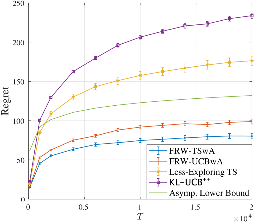
Refer to caption
(a) Instance μsuperscript𝜇\mu^{\dagger}
Refer to caption
(b) Instance μsuperscript𝜇\mu^{\ddagger}
Figure 4: Empirical regrets with abstention reward c=0.9𝑐0.9c=0.9 for different time horizons T𝑇T.

Next, we examine the impact of the abstention reward c𝑐c by assessing the performance of FRW-TSwA and FRW-UCBwA for different c𝑐c, while keeping the time horizon T𝑇T fixed at 10,0001000010,000. The experimental results for bandit instances μsuperscript𝜇\mu^{\dagger} and μsuperscript𝜇\mu^{\ddagger} are shown in Figure 5.

Within each sub-figure, a pattern emerges. As the abstention reward c𝑐c increases, the empirical average cumulative regret initially remains relatively stable and starts to decline once c𝑐c crosses a certain threshold, eventually stabilizing around a small value. These observations are consistent with our theoretical expectations. Specifically, when the abstention reward c𝑐c is lower than the smallest mean reward among the arms, the agent derives no benefit from opting for the abstention action over selecting an arm. On the other hand, when the abstention reward c𝑐c exceeds the highest mean reward of the arms, abstention becomes the optimal decision and its reward is even superior to choosing the best arm. In this specific scenario, it is possible to achieve a regret of o(logT)𝑜𝑇o(\log T); see Remark 4.2 for further insights.
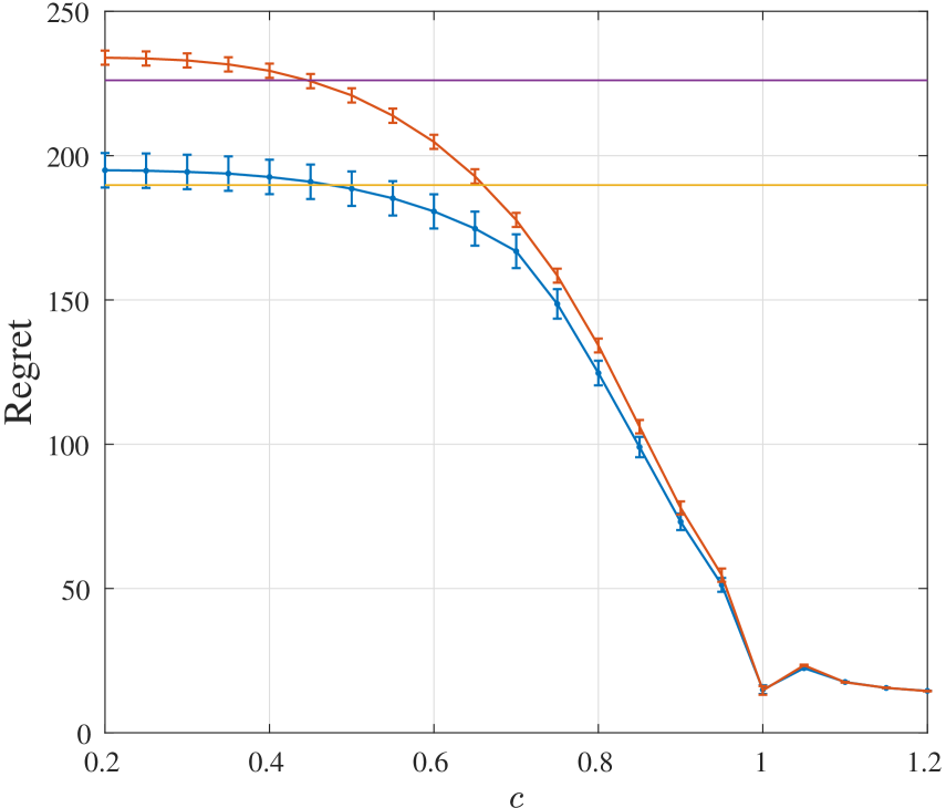
Refer to caption
(a) Instance μsuperscript𝜇\mu^{\dagger}
Refer to caption
(b) Instance μsuperscript𝜇\mu^{\ddagger}
Figure 5: Empirical regrets with time horizon T=10,000𝑇10000T=10,000 for different abstention rewards c𝑐c.

E.2 Random Instances

In this subappendix, we present additional numerical experiments, using random instances with large numbers of arms. The construction of these random instances mirrors the method in Jin et al. (2023). Specifically, for a given number of arms denoted by K10𝐾10K\geq 10, we set μ1=1subscript𝜇11\mu_{1}=1 and μi=0.7subscript𝜇𝑖0.7\mu_{i}=0.7 for i{2,3,,10}𝑖2310i\in\{2,3,\ldots,10\}, while μiUnif[0.3,0.5]similar-tosubscript𝜇𝑖Unif0.30.5\mu_{i}\sim\operatorname{Unif}[0.3,0.5] for i[K][10]𝑖delimited-[]𝐾delimited-[]10i\in[K]\setminus[10].

For the sake of simplicity in presentation, we focus on the fixed-regret setting, examining two choices of K𝐾K, namely, K=20𝐾20K=20 and K=30𝐾30K=30. The empirical averaged cumulative regrets with abstention regret c=0.1𝑐0.1c=0.1 for different time horizons T𝑇T are shown in Figure 6, while the experimental results with time horizon T=10,000𝑇10000T=10,000 for different abstention rewards c𝑐c are illustrated in Figure 7.

It is evident that the findings in Figures 6 and 7 closely resemble those in Figures 2 and 3. Notably, FRW-TSwA outperforms Less-Exploring TS which is not tailored to the setting with the abstention option.
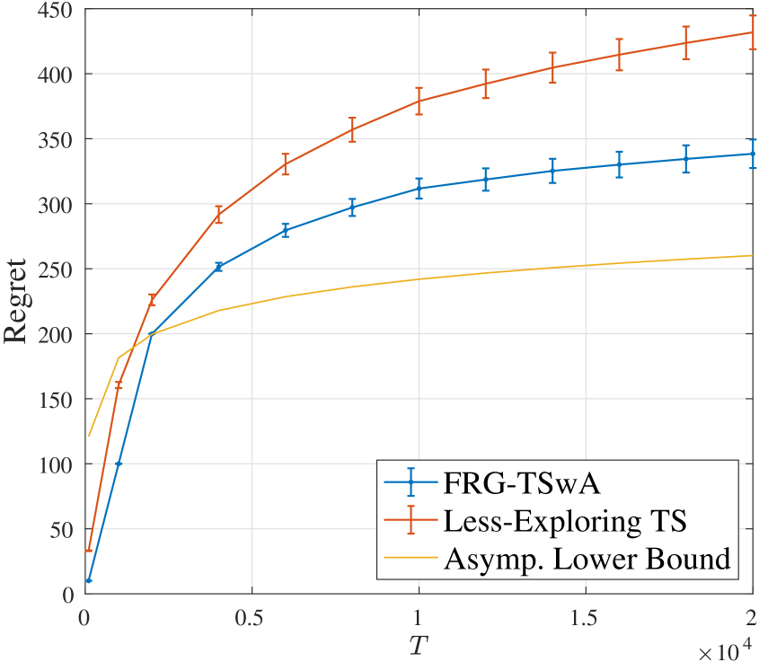
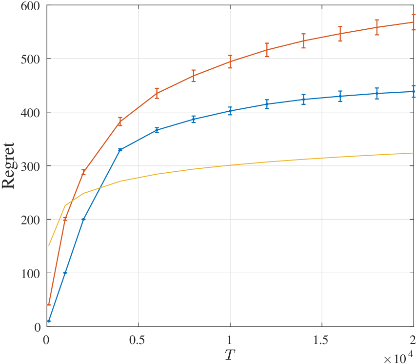
Refer to caption
(a) K=20𝐾20K=20
Refer to caption
(b) K=30𝐾30K=30
Figure 6: Empirical regrets with abstention regret c=0.1𝑐0.1c=0.1 for different time horizons T𝑇T.
Refer to caption
(a) K=20𝐾20K=20
Refer to caption
(b) K=30𝐾30K=30
Figure 7: Empirical regrets with time horizon T=10,000𝑇10000T=10,000 for different abstention regrets c𝑐c.