Accelerating Convergence of Stein Variational Gradient Descent via Deep Unfolding
Abstract
Stein variational gradient descent (SVGD) is a prominent particle-based variational inference method used for sampling a target distribution. SVGD has attracted interest for application in machine-learning techniques such as Bayesian inference. In this paper, we propose novel trainable algorithms that incorporate a deep-learning technique called deep unfolding, into SVGD. This approach facilitates the learning of the internal parameters of SVGD, thereby accelerating its convergence speed. To evaluate the proposed trainable SVGD algorithms, we conducted numerical simulations of three tasks: sampling a one-dimensional Gaussian mixture, performing Bayesian logistic regression, and learning Bayesian neural networks. The results show that our proposed algorithms exhibit faster convergence than the conventional variants of SVGD.
Index Terms:
particle-based variational inference, Stein variational gradient descent, deep learning, deep unfoldingI Introduction
Bayesian estimation is a probabilistic inference based on the Bayesian interpretation of probability[1]. Unlike the traditional maximum-likelihood estimation, Bayesian estimation maximizes the posterior probability calculated using the Bayes’ theorem from the likelihood and prior distribution corresponding to a hypothesis involving unknown variables. This approach is a powerful means of expressing prior information in terms of probability and facilitates not only the estimation but also prediction of new data. However, the posterior distribution is generally difficult to evaluate analytically because its normalization constant contains multiple integrals of random variables. This computational difficulty has been a long-standing issue in various research fields such as machine learning and signal processing [2]. To circumvent it, Markov-chain Monte-Carlo (MCMC) methods have been widely used in Bayesian estimation as approximate sampling methods for the posterior distribution[3]. For instance, the Hamiltonian Monte Carlo (HMC) method enhances the sampling efficiency through physics-inspired proposals [4], while the no-U-turn sampler [5] optimizes step selection in the HMC method. These recent MCMC methods reduce the inherent computational complexity of Bayesian estimation. However, MCMC methods still involve high computational costs because they serially update samples until the sample distribution is close to the target distribution. As a result, MCMC methods usually require long relaxation times, especially if the distribution lies in the high-dimensional space.
Recently, particle-based variational inference (ParVI) has been proposed to improve the convergence speed and sampling efficiency. Unlike MCMC methods, ParVI approximates the distribution based on the relative frequency distributions of the particles representing the samples. It updates the particles to minimize the Kullback–Leibler (KL) divergence from the target distribution. Stein variational gradient descent (SVGD)[6] is a representative ParVI algorithm, which uses a kernel function. The nonparametric nature of ParVI enhances its flexibility, resulting in particle efficiency better than that of the MCMC methods. In addition, ParVI algorithms, including SVGD, are closely related to the Wasserstein gradient flows [7]. A drawback of ParVI is its slow convergence speed, which depends on the initial and target distributions. In addition, minimizing the KL divergence is usually a nonconvex optimization. The fact suggests that gradient-based ParVI methods such as SVGD may converge to suboptimal solutions, leading to insufficient sampling of the target distribution. Although the performance of the algorithm depends on the choice of its internal parameters, the parameters are usually tuned in a heuristic manner.
The combination of deep learning and iterative algorithms has recently been attracting great interest. The deep-learning technique called deep unfolding (DU), in particular, enables the training of the internal parameters of an iterative algorithm, improving its convergence speed and performance[8]. In DU, the iterative process of an algorithm is unfolded in the temporal direction and trainable parameters are embedded in the unfolded structure. These parameters are learned through standard deep-learning techniques such as back propagation and stochastic gradient descent if the unfolded algorithm consists of differentiable processes. This approach has been confirmed to enhance the convergence performance of the algorithms [9, 10] and has been applied in various fields associated with signal processing [11, 12].
In this paper, we examine the application of DU to ParVI to improve the convergence speed and sampling performance. Specifically, we focus on SVGD and propose a deep-unfolded SVGD (DUSVGD) method, whose internal step-size parameters are learnable. Furthermore, inspired by the Chebyshev step[13], which is a step-size sequence for gradient descent, we propose a Chebyshev step-based DUSVGD (C-DUSVGD) algorithm. The number of trainable parameters of C-DUSVGD is only two, whereas that of DUSVGD is a constant with respect to the number of particles and dimension of variables. Finally, we numerically examine the performance of the proposed methods. Namely, we perform three different tasks: sampling a multimodal distribution, performing Bayesian logistic regression, and learning a Bayesian neural network.
The remainder of this paper is organized as follows. Section II briefly reviews SVGD, DU, and the Chebyshev step. Section III describes DUSVGD and C-DUSVGD and Sec. IV evaluates their performance. Section V concludes the paper.
II Preliminaries
In this section, we briefly review the previous studies related to this paper.
II-A Stein Variational Gradient Descent
SVGD is a ParVI algorithm that estimates a target distribution by minimizing the KL divergence between the distribution of particles in SVGD and the target distribution. Here, we briefly describe the SVGD algorithm[6].
SVGD uses a set of particles to approximate the -dimensional target distribution . The empirical distribution of the particle set is represented by (), where is the Dirac delta function. The particles are independently and identically distributed random variables from an initial distribution , and are iteratively updated according to the following equation:
| (1) |
where represents the vector-valued function indicating the direction of particle update and is the step size of the -th iteration (). The distribution followed by (1) is denoted as . In SVGD, is set to the direction that minimizes the KL divergence . By setting as the function space to which belongs, the optimal update direction is given by
| (2) |
where is the Stein operator, defined as . This optimization problem can be solved by restricting to a unit ball of a vector-valued reproducing kernel Hilbert space defined by a positive definite kernel . Then, the optimal direction is given by
| (3) |
Consequently, SVGD is summarized to Alg. 1 as an iterative algorithm.
In [6], the radial basis function (RBF) kernel is used as the positive definite kernel. The RBF kernel is defined by
| (4) |
The parameter aims to stabilize the computation of the gradient (3) by ensuring that . In this paper, we use the RBF kernel (4) unless otherwise noted.
The drawback of SVGD is that the minimization of the KL divergence is a nonconvex optimization, in general, leading to convergence to a suboptimal distribution of particles. Further, the difficulty of sampling multinomial distributions with distant peaks depends on an initial distribution, using SVGD [14, 15]. In addition, the sampling and convergence performance apparently depend on the step-size parameter , which is usually chosen heuristically.
II-B Deep Unfolding
As described in Sec. I, DU is a deep-learning technique that unfolds an existing iterative algorithm and trains its internal parameters to improve its performance[8].
We explain the DU of gradient descent as an example. Let the objective function be . The update rule of gradient descent that minimizes the function, with the maximum number of iterations , is given by
| (5) |
where represents the step-size parameters. In DU, we consider learning through supervised learning. Let a minibatch be given by
| (6) |
where is the minibatch size, () is the initial point of gradient descent, and is the corresponding optimal solution. During learning epochs, the trainable step sizes are optimized by minimizing a proper loss function such as the mean-squared error between the output of gradient descent and optimal solution . The training process is summarized in Alg. 2.
In Alg. 2, we employ the so-called incremental training to avoid gradient vanishing[11]. In the training, we first train the unfolded algorithm for iteration. After epochs are fed, the number of iterations is set to two. Similarly, all parameters are trained in an incremental manner. Note that back propagation is applicable to learning parameters because all processes of the algorithm are differentiable, leading to a fast training process.
II-C Chebyshev Step
The Chebyshev step is a step-size sequence that accelerates the convergence speed of gradient descent [16]. The sequence is theoretically derived to understand the trained step-size parameters of the deep-unfolded gradient descent. Here, we briefly review the Chebyshev step. Let be a positive definite symmetric matrix and consider minimizing . The update rule of gradient descent with step sizes is given by . Let us assume that step sizes are trained and that the algorithm is executed by setting with , where represents the learned step sizes. Then, the update rule for in every iterations is given by (). Recall that the matrix is a function of . The Chebyshev step is obtained as a solution that minimizes the upper bound of the spectral radius , which relates to the convergence speed of gradient descent. Finally, the Chebyshev step is obtained as a reciprocal of the root of the Chebyshev polynomial of order . Assuming that the maximum and minimum eigenvalues of are and , respectively, the Chebyshev steps of length [16] are given by
| (7) |
for . The convergence rate of gradient descent with the Chebyshev step is proved to be smaller than that of the gradient descent with a constant step size, indicating that the Chebyshev step can accelerate the convergence speed as well as a deep-unfolded gradient descent.
III Proposed Method
As described in the last part of Sec. II-A, SVGD is regarded as a gradient descent that minimizes the KL divergence, which is a nonconvex function in general. Here, we propose novel DU-based SVGD algorithms that allow us to learn the step sizes adapted to a target distribution or dataset.
III-A DUSVGD
The convergence performance of SVGD depends on the step sizes . Similar to the deep-unfolded gradient descent, we consider making the step sizes learnable by applying DU to SVGD. Namely, in the update rule of particles ,
| (8) |
where are trainable step-size parameters for a given . In this paper, the trainable SVGD is called DUSVGD. Note that all particles share the same step size for each , although we can train according to the particle. This is because we make the number of trainable parameters constant with respect to the number of particles, , leading to a scalable and fast training process. The value of is fixed in advance. In the following, we repeatedly use the trained step sizes for . Namely, we set with (mod ) for any .
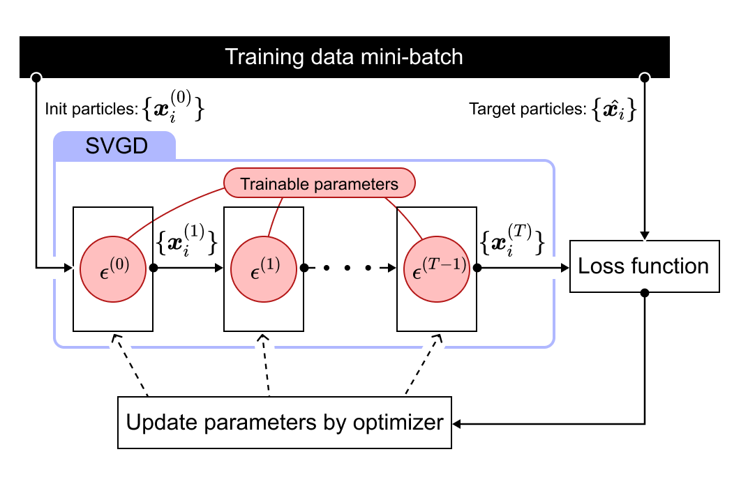
To prevent gradient vanishing in the training process of SVGD, the incremental training described in Sec.II-B is used. The architecture and training process of DUSVGD are depicted in Fig. 1. Note that we use a proper loss function depending on the task of DUSVGD, which is denoted in Sec. IV.
Note that the proposed DUSVGD is different from nueral variational gradient descent (NVGD) [17] that learns the function as a neural network. Although NVGD is more flexible than DUSVGD, the number of trainable parameters of NVGD is larger than that of DUSVGD, implying that the training cost of NVGD is more costly.
III-B C-DUSVGD
Let us consider a simple case where an SVGD with particle attempts to sample a target -dimensional Gaussian distribution with zero mean and variance-covariance matrix . Then, the update rule (1) with the RBF kernel is rewritten as because and hold when . This indicates that SVGD is equivalent to a gradient descent that minimizes a quadratic function, in this case. Notice that the setting is the same as that for the Chebyshev step, suggesting that the Chebyshev step gives (sub)optimal step sizes.
From this observation, we consider applying the Chebyshev step to SVGD. However, the Chebyshev step requires and , the minimum and maximum eigenvalues of the Hessian matrix at the solution for general KL divergence, which is computationally difficult to estimate. We alternatively consider training and based on DU. Namely, the update rule for particles is written as
| (9) | ||||
| (10) | ||||
| (11) | ||||
| (12) |
where and are trainable parameters. Equation (11) represents the Chebyshev step111The order of the Chebyshev step affects the performance of C-DUSVGD in general. In this paper, we use the Chebyshev step in the reverse order, which exhibits better performance than (7)., and parameters are defined by (9) and (10) to satisfy the condition . This trainable SVGD is named C-DUSVGD, in this paper. C-DUSVGD is advantageous when compared to DUSVGD in terms of the lower training cost because it has only two trainable parameters for any and , whereas DUSVGD is more flexible than C-DUSVGD for approximating target distributions.
In the training process of C-DUSVGD, we do not require incremental learning because gradient vanishing is not observed. C-DUSVGD is trained only by the output after iterations. The trained step sizes are used periodically for .
IV Numerical Experiments
To evaluate the performance of the proposed trainable SVGD algorithms, we executed numerical simulations of three different tasks: sampling a one-dimensional Gaussian mixture distribution, Bayesian logistic regression, and learning a Bayesian neural network. Trainable SVGD algorithms were implemented using PyTorch 2.0.0 [18] and learned using the Adam optimizer[19]. For comparison, we used SVGD with RMSProp [20], a commonly used optimization method, and SVGD with a fixed step size. Note that other samplers such as the HMC were omitted because their performance was overwhelmed by that of the SVGD [6].
IV-A Sampling of Gaussian Mixture Distribution
As a simple example, we applied SVGD to approximate a one-dimensional Gaussian mixture distribution. The probability density function of the target distribution was given by
| (13) |
where denoted the probability density function of the Gaussian distribution with mean and variance . The initial distribution of particles in the SVGD was set to , with the number of particles . The maximum number of iterations for training (C-)DUSVGD was set to , and the trained step sizes were used periodically. The dataset consisted of 1000 random numbers generated from (13), with 90% used for training and 10% for testing. The minibatch size was , with learning epochs for DUSVGD and for C-DUSVGD. As a loss function, we used the maximum mean discrepancy (MMD) [21]. MMD estimated the distance between two distributions and using sample sets and independently drawn from and , respectively. It was defined by
| (14) |
where represented the unit ball in the reproducing kernel Hilbert space corresponding to the positive definite kernel , and
| (15) |
where and were sample sets. In this experiment, the RBF kernel was used for MMD The learning rate for the Adam optimizer was set to for DUSVGD and for C-DUSVGD. The initial value of trainable parameters were for DUSVGD and for C-DUSVGD.
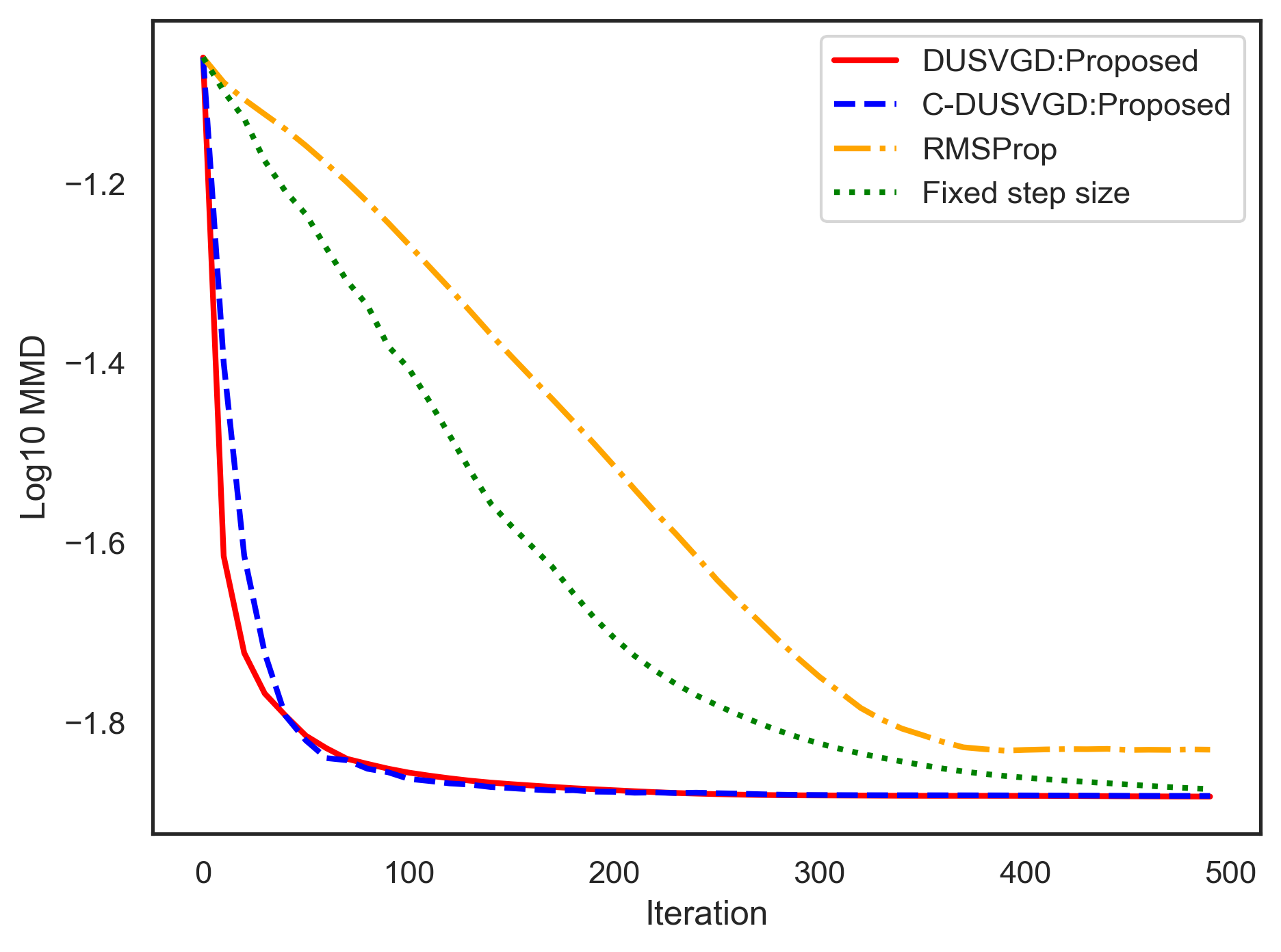
Figure 2 shows the MMD as a function of the number of iterations for DUSVGD, C-DUSVGD, SVGD with RMSProp (referred to as “RMSProp”), and SVGD with a fixed step size (referred to as “fixed step size”). MMD was calculated using randomly chosen samples and averaged over trials. In terms of the convergence performance, DUSVGD and C-DUSVGD, which learned the step sizes, converged faster than RMSProp and fixed step size. For example, the number of iterations required to achieve was approximately 20 for DUSVGD, 30 for C-DUSVGD, 280 for RMSProp, and 200 for fixed step size. This shows the effectiveness of learning the step size parameters of SVGD. The superiority of DUSVGD over C-DUSVGD suggests that the flexibility of the architecture affects the convergence performance.
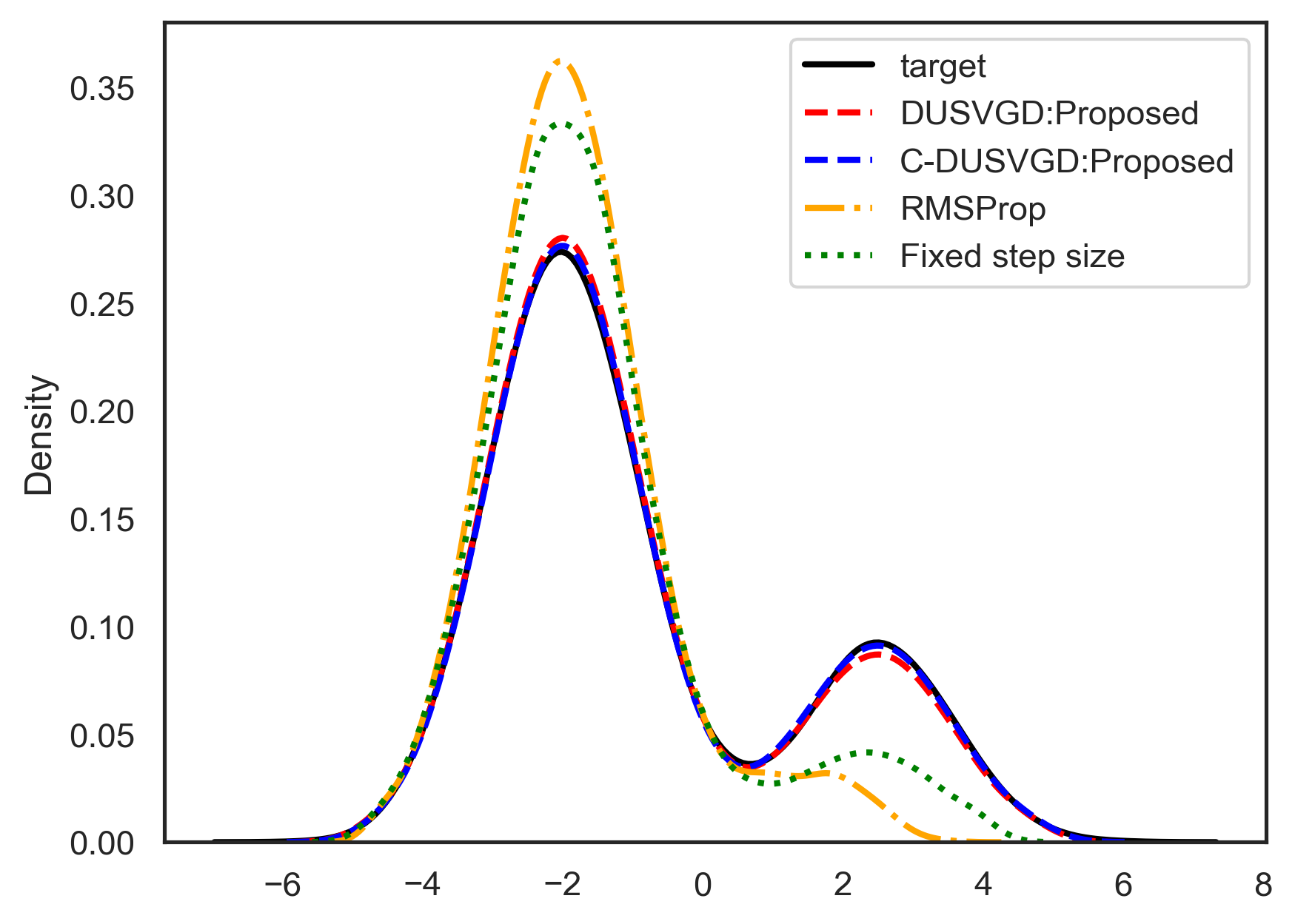
Figure 3 shows the distribution of particles of SVGD algorithms after iterations. We applied kernel density estimation using the RBF kernel of bandwidth to estimate the particle distribution. We found that DUSVGD and C-DUSVGD could approximate the distribution more accurately with fewer iterations than SVGD with RMSProp and fixed step size
.
IV-B Bayesian Logistic Regression
Next, we consider a more practical problem using real data. Here, we apply SVGD to the Bayesian logistic regression for a binary classification dataset222https://www.csie.ntu.edu.tw/~cjlin/libsvmtools/datasets/binary.html. The observational data consists of class label and explanatory variables for each data point, where and . In the experiment, the target distribution for the regression coefficients is modeled as a posterior distribution used in the previous study [22]. The target distribution is given by
| (16) | ||||
| (17) | ||||
| (18) |
where is a Gamma distribution defined by
| (21) | ||||
| (22) |
In the model, represents a precision parameter following the Gamma distribution with hyperparameters and . As a Bayesian estimation, (16) and (17) represent the prior distributions and corresponds to the likelihood. Here, represents a vector of all class labels, while denotes a matrix comprising all observed data points. SVGD approximates the target posterior distribution . The values of hyperparameters are set to and .
In SVGD, each particle was a -dimensional random variable containing the values of and . In the experiment, particles were used, which were initialized by prior distributions. The number of iterations for training (C-)DUSVGD was set to , and the learned step sizes were used periodically. 80% of data points were used for training and the remaining 20% for testing. The minibatch size was , with learning epochs for DUSVGD and for C-DUSVGD. The cross-entropy function between the true and estimated class labels was used as the loss function because the true posterior distribution was unknown in this case. Thus, the loss function is defined by
| (23) |
where is the number of training data, is a true class label in training data, and is the corresponding estimated class label. The learning rate for the Adam optimizer was set to for DUSVGD and for C-DUSVGD. The initial value of trainable parameters were for DUSVGD and for C-DUSVGD.
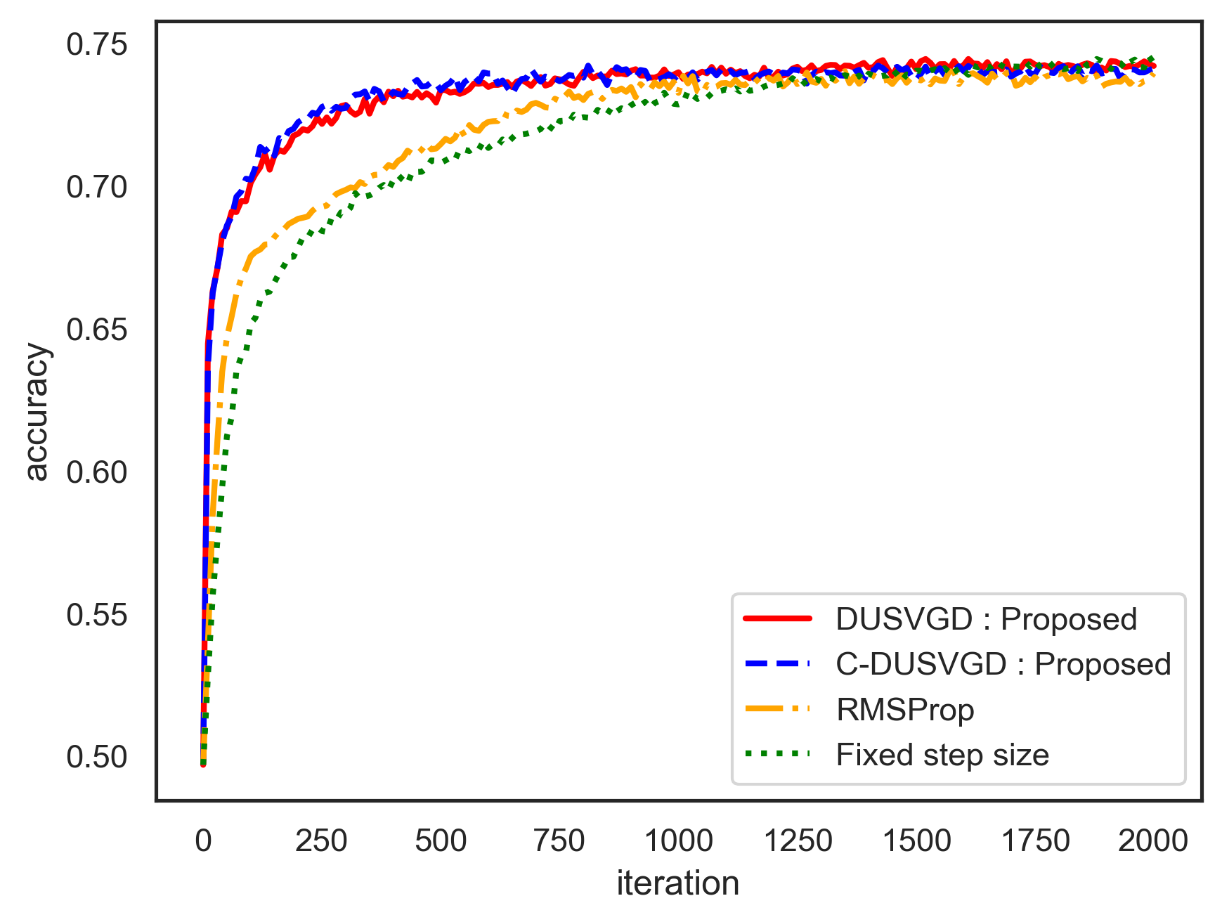
Figure 4 shows the dependency of the accuracy on the number of iterations for DUSVGD, C-DUSVGD, RMSProp, and fixed step size in the Bayesian logistic regression problem. In the figure, the accuracy of the label prediction was averaged over 30 trials. In terms of convergence performance, it was observed that DUSVGD and C-DUSVGD showed reasonable improvement compared to the other SVGD. For instance, the accuracy at 500 iterations was approximately 73.3% for DUSVGD, 73.4% for C-DUSVGD, 71.6% for RMSProp, and 70.7% for fixed step size. The result shows that the proposed (C-)DUSVGD exhibits reasonable performance gain compared to the existing SVGD, even for Bayesian logistic regression with real data. It is emphasized that the training was executed with only iterations, resulting in an efficient training cost.
IV-C Learning Bayesian Neural Networks
As the second numerical experiment with real data, we examined the application of learning Bayesian neural networks for a regression dataset333https://www.cs.toronto.edu/~delve/data/boston/bostonDetail.html. The training data consisted of a target value and corresponding -dimensional input vectors , where and . In the experiments, we assumed that the target values were obtained as , where was a two-layer fully connected neural network with 50 units, ReLU activation function in the middle layer, and identity activation function in the output layer. Unlike typical neural networks, the model contained a Gaussian noise following . Our task was to learn the weight matrix as a Bayesian neural network. Namely, we assumed the weights were random variables and introduced the following probabilistic model.
| (24) | ||||
| (25) | ||||
| (26) | ||||
| (27) |
where and were precision parameters following Gamma distributions, and , and were the hyperparameters of the Gamma distributions. The distributions (24), (25), and (26) represented prior distributions, and (27) represented the likelihood. SVGD approximated the target posterior distribution to obtain the weights of the neural network. In this sense, SVGD was used as an optimizer for the Bayesian neural network.
In the experiment, the values of hyperparameters were set to and . In SVGD, particles were initialized by random numbers drawn from the prior distributions. The maximum number of iterations for learning (C-)DUSVGD was set to , and the learned step sizes were used periodically. We used 90% of data points for training and the remaining 10% for testing. The minibatch size was , with learning epochs for DUSVGD and C-DUSVGD. As a loss function, we used the mean squared error between the output and true . The learning rate for the Adam optimizer was set to for DUSVGD and for C-DUSVGD. The initial value of trainable parameters were for DUSVGD and for C-DUSVGD.
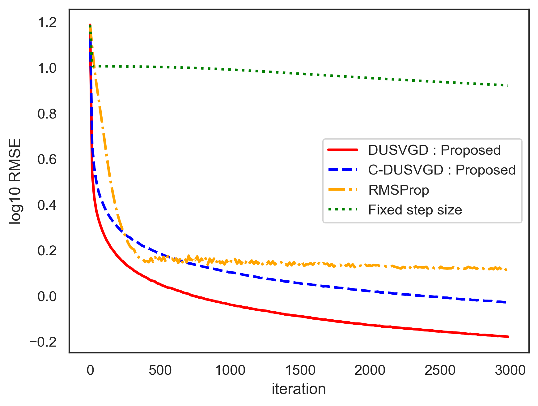
Figure 5 shows the root mean squared error (RMSE) as a generalization loss, as a function of the number of iterations for DUSVGD, RMSProp, and fixed step size in Bayesian neural networks. RMSE was estimated by averaging over 10 trials. It was found that DUSVGD and C-DUSVGD improved the convergence speed and approximation performance compared to the other methods. For example, the value of after iterations was approximately for DUSVGD, for C-DUSVGD, for RMSProp, and for fixed step size. In addition, we found that the RMSE of RMSProp stopped at approximately , implying that its particle distribution converged to a suboptimal distribution, possibly because of the nonconvexity of the KL divergence minimized by SVGD. In contrast, the RMSE of (C-)DUSVGD continued decreasing after iterations. This indicated that learning step size parameters could avoid convergence to undesired local minima. Compared to that of C-DUSVGD, the RMSE performance of DUSVGD was reasonably better, suggesting that the performance depended on the flexibility of the unfolded algorithms.
It is emphasized that training SVGD for optimizing Bayesian neural networks is regarded as meta-learning[23]. The proposed trainable SVGD algorithms show remarkable performance improvement, although they are trained with only iterations. The result implies that the proposed algorithms are promising meta-learning techniques for Bayesian neural networks.
V Conclusion
In this paper, we proposed DUSVGD and C-DUSVGD by applying DU to SVGD, a representative ParVI algorithm for sampling a target distribution. The numbers of trainable parameters of DUSVGD and C-DUSVGD were and , respectively, both of which were independent of the dimension of a target distribution and the number of particles. These algorithms enabled us to tune step sizes flexibly via deep-learning techniques, according to the task and data set. In particular, C-DUSVGD employed the theory of the Chebyshev step, resulting in the lowest number of trainable parameters. We conducted numerical simulations for three tasks to examine the proposed (C-)DUSVGD. For sampling from the Gaussian mixture distribution and Bayesian logistic regression problem, DUSVGD and C-DUSVGD improved the convergence speed compared to classical SVGD. Furthermore, the result of learning Bayesian neural networks indicated that training (C-)DUSVGD improved not only the convergence speed but also the learning performance. In the experiments, (C-)DUSVGD were learned with the first iterations, and their learned parameters were used repeatedly. This greatly reduced the training costs of the proposed trainable SVGD, which was applicable to meta-learning. Future work may include applying DU to improve ParVI methods designed for accelerating convergence [7].
References
- [1] G. E. Box and G. C. Tiao, “Bayesian Inference in Statistical Analysis,” John Wiley & Sons, 2011.
- [2] D. M. Blei, A. Kucukelbir, and J. D. McAuliffe, “Variational Inference: A Review for Statisticians,” Journal of the American Statistics Association, vol. 112, no. 518, pp. 859-877, 2017.
- [3] D. Luengo, L. Martino, M. Bugallo, V. Elvira, and S. Särkkä, “A Survey of Monte Carlo Methods for Parameter Estimation,” EURASIP Journal of Advances in Signal Processing, vol. 2020, p. 25, 2020
- [4] S. Duane, A. D. Kennedy, B. J. Pendleton, and D. Roweth, “Hybrid Monte Carlo,” Physics Letters B, vol. 195, no. 2, pp. 216–222, 1987.
- [5] M. D. Hoffman and A. Gelman, “The No-U-Turn Sampler: Adaptively Setting Path Lengths in Hamiltonian Monte Carlo,” Journal of Machine Learning Research, vol. 15, no. 1, pp. 1593–1623, 2014.
- [6] Q. Liu and D. Wang, “Stein Variational Gradient Descent: A General Purpose Bayesian Inference Algorithm,” Advances In Neural Information Processing Systems, pp. 2378-2386, 2016.
- [7] C. Liu, J. Zhuo, P. Cheng, R. Zhang, and J. Zhu, “Understanding and Accelerating Particle-based Variational Inference," International Conference on Machine Learning, pp. 4082-4092, 2019.
- [8] K. Gregor and Y. LeCun, “Learning Fast Approximations of Sparse Coding," International Conference on Machine Learning, pp. 399-406, 2010.
- [9] V. Monga, Y. Li, and Y. C. Eldar, “Algorithm Unrolling: Interpretable, Efficient Deep Learning for Signal and Image Processing," IEEE Signal Processing Magazine, vol. 38, no. 2, pp. 18-44, 2021.
- [10] N. Shlezinger, Y. C. Eldar, and S. P. Boyd, “Model-Based Deep Learning: On the Intersection of Deep Learning and Optimization," IEEE Access, vol. 10, pp. 115384-115398, 2022.
- [11] D. Ito, S. Takabe and T. Wadayama, “Trainable ISTA for Sparse Signal Recovery," IEEE Transactions on Signal Processing, vol. 67, no. 12, pp. 3113-3125,2019.
- [12] S. Takabe, M. Imanishi, T. Wadayama, R. Hayakawa, and K. Hayashi, “Trainable Projected Gradient Detector for Massive Overloaded MIMO Channels: Data-Driven Tuning Approach,” IEEE Access, vol. 7, pp. 93326-93338, 2019.
- [13] S. Takabe and T. Wadayama, “Chebyshev Periodical Successive Over Relaxation for Accelerating Fixed-Point Iterations,” IEEE Signal Processing Letters, vol. 28, pp. 907-911, 2021.
- [14] J. Zhuo, C. Liu, J. Shi, J. Zhu, N. Chen, and B. Zhang, “Message Passing Stein Variational Gradient Descent,” International Conference on Machine Learning, pp. 6018-6027, 2018.
- [15] F. D’Angelo and V. Fortuin, “Annealed Stein Variational Gradient Descent,” Symposium on Advances in Approximate Bayesian Inference,, 1-10, 2020.
- [16] S. Takabe and T. Wadayama, “Convergence Acceleration via Chebyshev Step: Plausible Interpretation of Deep-Unfolded Gradient Descent,” IEICE Transactions on Fundamentals of Electronics, Communications and Computer Sciences, vol. E105.A, no. 8, pp. 1110-1120, 2022.
- [17] L. L. di Langosco, V. Fortuin, and H. Strathmann, “Nueral Variational Gradient Descent,” Symposium on Advances in Approximate Bayesian Inference,, 1-17, 2020.
- [18] PyTorch: https://pytorch.org/.
- [19] D. P. Kingma and J. L. Ba, “Adam: A Method for Stochastic Optimization,” arXiv:1412.6980, 2014.
- [20] T. Tieleman and G. Hinton, “Lecture 6.5-rmsprop: Divide the Gradient by a Running Average of its Recent Magnitude,” COURSERA: Neural Networks for Machine Learning, 2012.
- [21] A. Gretton, K. M. Borgwardt, M. Rasch, B. Schoelkopf, and A. J. Smola, “A Kernel Method for the Two-Sample-Problem,” Advances in Neural Information Processing Systems, pp. 513-520, 2006.
- [22] S. Gershman, M. Hoffman, and D. Blei, “Nonparametric Variational Inference,” International Conference on Machine Learning, pp.235-242, 2012.
- [23] T. Hospedales, A. Antoniou, P. Micaelli, and A. Storkey, “Meta-Learning in Neural Networks: A Survey,” IEEE Transactions on Pattern Analysis and Machine Intelligence, vol. 44, no. 9, pp. 5149-5169, 2022.