The Neural Network First-Level Hardware Track Trigger of the Belle II Experiment

Abstract

We describe the principles and performance of the first-level (”L1”) hardware track trigger of Belle II , based on neural networks. The networks use as input the results from the standard Belle II trigger, which provides “2D” track candidates in the plane transverse to the electron-positron beams. The networks then provide estimates for the origin of the 2D track candidates in direction of the colliding beams (“$z$-vertex”), as well as their polar emission angles $\theta$. Given the $z$-vertices of the “neural” tracks allows identifying events coming from the collision region ($z\approx 0$), and suppressing the overwhelming background from outside by a suitable cut $d$. Requiring $|z|<d$ for at least one neural track in an event with two or more 2D candidates will set an L1 trigger. The networks also enable a minimum bias trigger, requiring a single 2D track candidate validated by a neural track with a momentum larger than 0.7 GeV in addition to the $|z|$ condition. The momentum of the neural track is derived with the help of the polar angle $\theta$.

1 Introduction

Searches for new physics with the Belle II detector [2], taking data at asymmetric-energy $e^{+}e^{-}$collider SuperKEKB[3], will require extremely high statistics to challenge the predictions of the Standard Model (SM). SuperKEKB, an upgrade of the legendary “$B$-factory” KEKB[4], is running now since 2019 and continues to produce increasing world-record luminosities, targeting 6 $\times$ 10³⁵ cm^-2s^-1, at the center-of-mass energy of 10.58 GeV. This collision energy corresponds to the mass of the $\Upsilon$(4S) resonance which decays predominantly into a pair of $B$ mesons, more precisely into $B^{+}B^{-}$ pairs or $B^{0}\,\bar{B}^{0}$ pairs in roughly equal numbers. In addition to the $\Upsilon$(4S) a “continuum” of the lighter mesons (mostly pions, kaons and $D$-mesons) is produced in the annihilation of electrons and positrons, which includes, among other less interesting quantum electrodynamics (QED) processes, the important two-body leptonic final states $\mu^{+}\mu^{-}$ and $\tau^{+}\tau^{-}$.

All the reactions mentioned above produce final state particles which have, apart from the decay products of some long-lived particles, their origin (“vertex”) within the small collision volume of the electron-positron beams (“interaction point” or “IP”). The IP region has a size of order micrometers in the two directions transverse to the beam direction (“$x,y$”, or “$r\phi$”) and a few millimeters along the beam (“$z$”) direction. There is, however, a sizeable “background” caused by interactions of the beam particles with the residual gas in the beam pipe (diameter 2 cm) or with the beam pipe itself, or with elements of the magnetic beam guiding and focusing system. When these interactions occur not too far from the IP, they may emit the particles produced in the collision into the Belle II detector and create signals similar to the desired annihilation events. This background is mainly characterized by particles created essentially close to the beam line ($|x|\approx|y|\approx$ 0), while having a vertex with a large displacement from IP ($|z|\gg 0$), typically of order several cm up to a meter.

At the IP of the Belle II detector the electron and positron bunches cross each other with a frequency of roughly 200 MHz (typically 2000 bunches of each particle type circulate in opposite directions in the rings of SuperKEKB with a circumference of 3 km). In any of the bunch crossings an interesting event might happen. Given the volume of the event data and the bunch crossing frequency of 200 MHz, it is completely impossible to read out the signals from the entire Belle II detector for each bunch crossing, i.e. each 5 ns. One rather builds up a so-called “trigger system” which identifies, from a reduced set of detector data, those bunch crossings containing “physically interesting” events.

As for the Belle experiment[5], Belle II ’s trigger system has two “levels”: The first level or “level 1” (“L1” for short) is hard-wired and deadtime-free. It uses special fast digital detector signals which are stored in a FIFO (“$f$irst $i$n $f$irst $o$ut”) pipeline and are subjected to selection algorithms implemented in “field-programmable gate arrays” (FPGAs). The pipeline can hold the L1 data for 5 $\mu$s, which defines the decision time for the L1 algorithms. There are basically four major detector components of the Belle II detector which contribute to the L1 trigger (see [2] for details). These are the electromagnetic calorimeter (ECL), the central drift chamber (CDC), the K-long-muon detector (KLM) and the time-of-propagation detector (TOP). The main L1 trigger algorithms are executed with the ECL and CDC data, assisted by the KLM and TOP systems. A positive L1 decision is taken by an OR of the main trigger processors. Once an L1 trigger is asserted, the complete detector data of that corresponding bunch crossing are read out. After kinematic reconstruction of the charged and “visible” neutral particles in the final state, a high-level software trigger (HLT) makes the final decision and the data of the accepted events are stored on permanent media for subsequent physics analyses. One of the obvious criteria applied by the HLT is to accept events only when the majority of the charged particles come from the IP region, i.e. $|z|<\cal{O}$(1 cm).

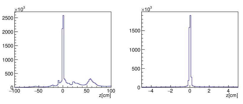
Figure 1: Left: Distribution of the $z$-positions in centimeters of reconstructed tracks from Belle II , over the entire $z$ range. Right: same as left, but with higher resolution in $z$ around the IP. The events from $e^{+}e^{-}$collisions contribute only about 20% of all events. The data are from the running in early 2021, before the launch of the $z$-Trigger .

In Belle II , the L1 trigger for charged particles (“tracks”) is derived from the CDC. In the first two years of data taking the L1 track trigger was using tracks in the $r\phi$ plane, perpendicular to the $z$-direction of the colliding electron-positron beams. However, this “2D” track trigger cannot discriminate true annihilation events ($|z|$ small) from background tracks originating far from the IP ($|z|$ large). Making the L1 track trigger sensitive to charged particles which originate close to the IP, while keeping the trigger rate within acceptable bounds, is of crucial importance for the efficient data taking, especially at rising luminosities: An unfortunate side effect of the high luminosity is a much higher level of background, dominated by Touschek scattering [6, 7] and beam-gas interactions. This background produces a high rate of undesirable events with tracks mostly originating outside of IP. The “problem” of the 2D track trigger can be seen in Fig.1, where the majority of the events triggered come from background outside of the IP. On the left one clearly recognizes the “obstacles” for the beam approaching the IP, located at $z=0$: The peaks at about $\pm$ 60 cm are caused by the tips of the last focusing quadrupoles QCSL and QCSR, the excess tracks around $\pm$ 20 cm are from the crotch part of the beampipe, and the peaks around $\pm$ 10 cm are from the stainless-steel cooling supports of the pixel vertex detector. The events in the figure have been triggered by the standard 2D trigger. With rising backgrounds the 2D trigger cannot be maintained without an additional constraint, namely adding the third track dimension and providing an estimate for the $z$-vertex of the tracks.

We report here on a novel L1 track trigger for Belle II , based on neural networks, which estimates in addition to the $r\phi$ of the 2D tracks their $z$-impact along the beam direction (“$z$-Trigger ”). Due to their inherent parallel architecture, neural networks are ideally suited for solving complex pattern recognition tasks within a predictable computation time, which is typically of order microseconds in modern FPGAs. Furthermore, the adaptive approach of the neural trigger, being trained with real data, will ensure an optimal performance under rising background conditions.

This is not the first time that neural networks have been actively used in high energy physics experiments: A level 2 neural network trigger[8], performing event classification according to physics criteria, was launched in the H1 experiment at the HERA accelerator (DESY, Hamburg), and very successfully contributed to the physics of electron-proton reactions.

The present paper is structured as follows: We will first describe the principles of the neural method determining the origin in the $z$-direction of the tracks in an event. In section 2 we outline the principles of operation of the neural network trigger and in section 3 we describe the preparation of the input to the neural networks and their training. Section 4 presents the implementation of the neural algorithm (preprocessing and network calculations) in hardware. In section 5 we present the performance of a new trigger concept, in particuar the minimum bias Single Track Trigger (“STT”), which requires one neural track with momentum above a certain threshold. This trigger was implemented in the Global Decision Logic (“GDL”) of Belle II starting in March 2021 and is now the main L1 track trigger for low multiplicity events. In section 6 we describe ongoing developments and improved strategies for the neural trigger towards target instantaneous luminosities, and summarize in section 7.

2 Principle of the Neural z-Trigger

As mentioned in the previous section, charged particles are triggered with the help of the CDC. The chamber, with inner (outer) radius of $r\approx$ 16 (113) $\mathrm{cm}$, is equipped with 56 cylindrical layers of axial and stereo wires, . The CDC contains about 15.000 sense wires, centered in drift cells with a size of 2 cm. Six adjacent wire layers are combined to form nine so-called super-layers (“SL”). The innermost SL has eight layers with smaller (half-size) drift cells to cope with the increasing background towards smaller radii.

The wire directions for each of the nine SLs are alternating between axial (“A”) orientation, aligned with the solenoidal magnetic field ($z$-axis), and stereo (“U”,“V”) orientations. The stereo wires are skewed by angles between 45.4 and 74 mrad in positive (U) and negative (V) directions with respect to the $z$-axis, thus enabling a measurement of the polar angles of the tracks.

In contrast to offline track reconstruction using all 56 wire planes, the track finding for the trigger is based on a reduced set of sense wires in each of the nine SLs (5 axial and 4 stereo SLs). This subset of wires is selected using hard-wired so-called track segments (“TS”), which combine wires in five adjacent layers within a SL to patterns similar to hour-glass shapes (see fig. 2, right side, for the TS in SL0 the wire set is shown on the left side). For a TS to “fire”, its wires have to satisfy plausible patterns originating from traversing tracks. The central wire (“priority wire”) defines the spatial position of the TS. In case the central priority wire is not hit, two so-called “secondary priority wires” are defined, which take the role of the priority wire. The set of priority wires form the basis of the track reconstruction within the trigger logic. Introducing the TSs also provides an extremely powerful suppression of random noise in the CDC. The set of possible TS patterns is realized for fast access in look-up tables (“LUT”), which are synthesized statically during design-time.

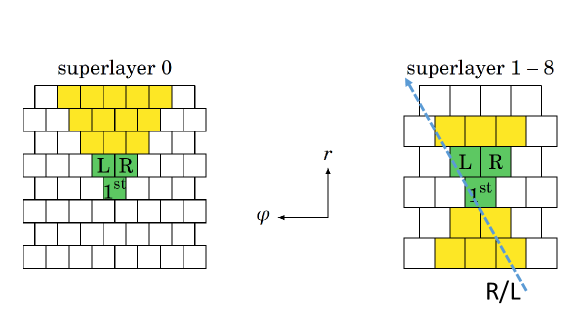
Figure 2: Left: TS of the innermost (axial) SL of the CDC consisting of 15 drift cells, arranged in triangular shape. Right: TS in the other eight SLs consisting of 11 drift cells in hour-glass shape. The drift cells used for the TS are marked in yellow. For each TS the wire marked as “1st” is called the ”priority wire”.

In the very early version of the CDC track trigger the priority wires in the TSs from the five axial SLs are combined to find tracks in the plane transverse to the beam direction (“$r\phi$ plane”). These tracks are called “2D tracks” in the following. Apart from the geometrical position of the priority wires, their drift time with a resolution of 2 ns is provided by the CDC front end electronics. Based on the pattern of the wires with non-zero signals within a given TS, the passing of the particle on the right or left side of the priority wire is estimated, leading to a “signed” drift time . Using the positions of the priority wires of the axial TSs, improved by the drift time , the track finding is done using Hough transform techniques [9]. The Hough method assumes the track origins at ($x=0,y=0$) in the $r\phi$ plane and returns a set of 2D track candidates, which are defined by their azimuthal emission angles $\phi$ at the origin and their track curvatures $\omega=1/R$, where $R$ is the radius of the track orbit in the $r\phi$ plane. At least 4 of the 5 axial TSs are required in the Hough transform to establish a 2D track candidate.

A seemingly “natural” method for a trigger processor yielding tracks in three dimensions would be to use the 2D tracks found via Hough transformation and apply track fitting algorithms by adding the priority wire information from the stereo TSs in the various SLs. However, the combinatorics and fitting with adequate precision in iterative processes with non-deterministic execution times make the realization in a trigger application very difficult.

We have chosen an alternative approach for the track reconstruction in three dimensions at L1, based on artificial neural networks. Neural networks are excellent candidates for the implementation of triggers in hardware: The motivation for the neural $z$-Trigger is to provide a fast, fixed latency measurement of the $z$-vertex with sufficient precision in order to separate events from IP from those further away. A typical resolution of $\cal O$(5 cm) or better would be required to reject the dominating background from outside of the IP (see fig. 1). Using only the sense wire positions would result in a resolution exceeding 10 cm. The crucial step forward therefore is to use the drift time in addition to the topological information of the priority wire in the TSs. This additional information increases the space point precision by roughly an order of magnitude.

In our initial studies, based on Monte-Carlo simulations[10, 11, 12], the neural approach, performing a regression task, provided a sufficiently accurate estimate of the track $z$-vertex without explicit reconstruction. The first step of the algorithm is to prepare the input data to the networks, choosing a set of significant variables and subjecting them to suitable preprocessing.

Starting from the tracks found by the standard 2D system, each candidate provides, in addition to the track curvature $\omega$ and the azimuthal emission angle $\phi$, the positions and signed drift times for the priority wires in each associated TS. In a second step, a set of possible stereo TSs associated to each of the 2D tracks is selected and the stereo TS with the shortest drift time is chosen for each of the four stereo SLs.

At present (for planned extensions see later in this paper), the inputs to the neural $z$-Trigger are the axial TSs from the 2D baseline trigger and the associated stereo TSs. For each of the up to 9 priority wires three variables are calculated (“preprocessing”, see next section) which are fed into a single hidden layer feed-forward neural network. The two outputs of the network are the $z$ position and polar angle $\theta$ of a “neural” track. For a given event a number $n$ of 2D candidates will exist, leading to a number $\leq n$ of neural tracks.

The scheme for triggering charged particles with the Belle II detector is as follows: A neural track with typically $|z|<15$ cm is required for all standard $\geq 2$ track triggers in the Global Reconstruction Logic (GRL). In addition, using the estimate of the polar angle $\theta$, the momentum of the tracks can be calculated. This is used to enable a trigger requiring only one single track. This ”Single Track Trigger (STT)” requires $|z|<15$ cm, and a momentum $p>0.7$ GeV.

The STT can be considered as a minimum bias trigger in the sense that only a single track in an event is required within the acceptance of the CDC. Since any physical event with charged particles in the final state has at least two reconstructed tracks, the STT opens up the full phase space for the second and further tracks in the event. This is especially important for low multiplicity events such as $\tau$ pair production, certain dark matter signatures, or processes like $e^{+}e^{-}$$\rightarrow\pi^{+}\pi^{-}(\gamma)...$. The cross sections for the latter processes are important to better understand the muon $g-2$ anomaly[13].

3 Neural Architecture, Preprocessing, Training

The neural algorithms, yielding for each track in an event an estimate for the $z$-coordinate and the polar emission angle $\phi$, are executed on Field Programmable Gate Arrays (“FPGA”) in the CDC track trigger electronic boards (see next section). Due to latency limitations at L1 only about 350 ns are available for the execution of the neural algorithm, including input variable preprocessing and delivery of the output to the GRL. Therefore only single-hidden-layer feed-forward network architectures were considered.

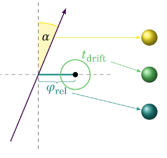
Figure 3: Preprocessing of input variables to the neural network: for each TS contributing to a neural track, a triple of variables is prepared, which give the crossing angle $\alpha$ of the track candidate through the TS, the angle $\varphi_{\rm rel}$ of the priority wire, and the signed drift time (see text).

The inputs to the neural networks consist of triples of variables derived for each priority wire in the associated TS for each of the nine SLs (shown in fig. 3). The triple of variables consists of the track crossing angle $\alpha$, the drift time $t_{\rm drift}$ and the relative azimuth angle $\varphi_{\rm rel}$. The crossing angle $\alpha$ is the inclination (or zenith) angle of the track passing the TS (see also fig. 2 for illustration). The angle $\varphi_{\rm rel}$ is given by the difference of the priority wire position in azimuth, $\phi_{\rm pw}$, and the value $\phi_{\rm extr}$ extrapolated from the Hough parameters $\phi$ and $\omega$ of the 2D track, measured at the end plate of the CDC. For the axial TSs this angle is usually close to zero. Then in each of the stereo SLs the TS candidates are selected using look-up tables (LUT), pre-determined from fully reconstructed tracks prior to the network training. This set of possible stereo TS candidates is defined within a range $\Delta\phi$ around the mean value $\phi_{\rm mean}$ of the two axial TS sandwiching the stereo SL. From this set the stereo TS with the shortest drift time is chosen, yielding the value $\varphi_{\rm rel}=\phi_{\rm pw}-\phi_{\rm mean}$ for the priority wire in the chosen stereo TS, again measured at the end plate of the CDC.

The drift times within the individual CDC drift cells containing the priority wires are determined in the following way: The CDC front end supplies a free-running counter encoding the arrival times of the charge avalanches at the wires with a precision of 2 ns. The smallest value of the counters from all the CDC wires would define the time of passage $t_{0}$ of particles through the CDC which is used in the offline reconstruction. Due to the limited number of wires for the trigger, however, no global $t_{0}$ is available. We have therefore chosen the method of “self timing”, looking for the smallest counter value $t_{\rm min}$ in the set of priority wires associated with the neural track candidate. This value is then subtracted from the timing counters in all the associated priority wires, yielding the unsigned drift times . The right-left (R/L) ambiguities for the drift times are lifted again by pre-determined LUT, analyzing the hit patterns in the TSs from a set of simulated tracks spanning a wide range of momenta and emission angles. Note that the patterns do not depend on the $z$-origin of the tracks. Whenever a clear decision can be made for the track passing right (left) from the priority wire, the drift time is assigned to a negative (positive) value (see fig. 2). In the case no decision can be made, the drift time is set to zero (“track passing close to the wire”), irrespective of the size of the drift time . The third input of the triple is the crossing angle $\alpha$ of the track through the TS. This quantity is derived from the Hough maxima $\phi$ and $\omega$ and the known radial position of the priority wires.

Since there are nine SLs (5 axial and 4 stereo) the number of inputs is $3*9=27$. The number of neurons in the hidden layer and the bit widths of the synaptic connections are determined by the available resources of the FPGAs. An optimum of 12 bits was found with 81 hidden nodes for the synaptic connections (more details see the hardware section). A schematic of the fully connected multi-layer-perceptron architecture is shown in fig. 4.

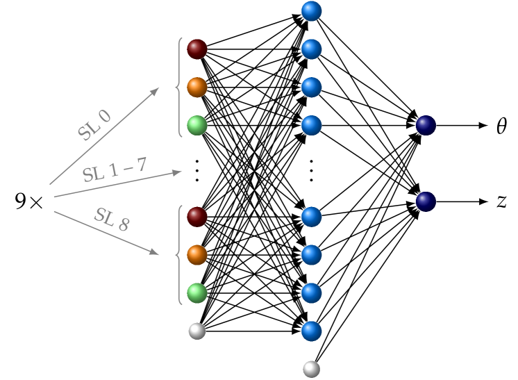
Figure 4: Sketch of chosen architecture for the fully connected feed-forward neural network. The input consists of 9 triples of data from the 9 SLs, giving a total of 27 inputs. Due to limitations of the available FPGAs only 81 nodes in a single hidden layer are implemented. Two output nodes provide the estimates for the $z$ origin of the track and its polar emission angle $\theta$.

The training of the networks is done with the target values $z_{\rm rec}$ and $\theta_{\rm rec}$ taken from the fully reconstructed tracks from an events sample recorded during the data taking. Since not always all TSs in the four stereo SLs are carrying signals (e.g. due to local inefficiencies in the CDC, or tracks missing the innermost or outermost stereo SLs), four so-called “expert networks”, each one for a specific missing stereo SL, are trained in addition to the network with complete stereo input (at least 3 out of the 4 stereo SLs are required to create a valid neuro track). It was found that the four experts associated with the missing stereo SLs, trained separately, are performing better than a single network with all cases included. A total of 5 networks, depending on the set of stereo TS in the data samples, are trained (“expert 0” to “expert 4”). For each of the 5 sets the same loss function $\mathcal{L}$ is defined:

$$\mathcal{L}=\sum{((z_{{\rm rec},j}-z_{{\rm net},j})^{2}+(\theta_{{\rm rec},j}-\theta_{{\rm net},j})^{2})}/N$$

where the sum runs over the $N$ tracks in the training sample. For numerical stability all input variables as well as the outputs are rescaled to a norm interval $[-1,+1]$ and the activation function is chosen as the hyperbolic tangent.

For the training of the first deployment of the neural trigger in the fall of 2020, the data collected during the spring of the year 2020 have been taken. At that time, the instantaneous luminosity was around $1.5\times 10^{34}$ cm^-2 s^-1. The training software used then was from the FANN library included in the basf2 software framework [14]. Typical $z$-resolutions around 5 cm were obtained from the initial training with the FANN library. This turned out to be sufficient for rejecting a large fraction of the off-IP events during the data taking in the year 2021 (see Sect. 5 below).

With rising luminosity and rising backgrounds towards the end of 2021 a new training was launched, based on the PyTorch library [15]. Here, we also include a second norm weight regularization into the loss function to punish excessively large weights and thus avoid overfitting issues. The loss function is minimized by Adam [16], a first order optimizer, using mini-batches. The gradients are calculated with the backpropagation algorithm implemented in PyTorch. Convergence is controlled by an independent validation data set. The sample sizes for training and convergence test are generally of order 300 k tracks. The training itself is done in floating point arithmetic. The transformation of all the inputs, outputs and network parameters to integers for the computations on the FPGAs is described in Sect. 4. The result was a real break-through, yielding a $z$-resolution of about a factor two better compared to the FANN training. Details on the performance of the new networks are given in Sect. 5.

4 Hardware Realization

The realization of the hardware [17] operating the $z$-Trigger is outlined in this section. It is organized into the aspects of integration, general architecture, configuration and test infrastructure. The integration describes the system locations within the CDC trigger system. Requirements to be fulfilled can be derived from the respective location. Following this, the overall architecture of the internal processing on the FPGA is introduced with implementation details, concentrating on the neural framework. The section concludes with the configuration of the architecture together with resulting characteristics, supplemented by testing procedures to identify functional problems.

4.1 Integration and Requirements

The neural trigger is part of the first level CDC sub-trigger system which imposes the requirement of being fully pipelined. The location of the neural trigger in the CDC trigger system is shown in fig. 5. The neural part is making ample use of the preceding processing modules which are organizing the wire information from the CDC front end electronics (CDC FEE) for further processing. To minimize the overall latency, the wire data are split in geometrical quadrants in the $(x,y)$ plane transverse to the beams, and the processing is done in parallel for all four quadrants. At the first stage, the track segments finders (aTSF, sTSF) concentrate the wire information in the axial TSs and stereo TSs (see previous sections). The axial TSs are used by the 2D finder (2DF) and build the 2D track parameters using Hough transforms. These parameters are sent together with their associated TSs to the neural trigger system (NNT). The stereo TSs on the other hand are sent directly to the neural trigger. There they have to be combined and related to the 2D candidate tracks. The selection of the related stereo segments is performed by an internal hit selection module. One of the inputs generated for each TS and directly used by the network is the drift time . In the original concept of the trigger, its calculation is based on an event time provided by the event time finder sub-system (ETF). However, this sub-system was not available at the time. To compensate this, an internal event time is calculated by setting the earliest priority time, out of all related TSs, as the event $t_{0}$ (see preceding section).

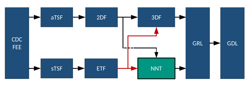
Figure 5: Integration of the neural trigger into the CDC trigger system. The various units are explained in the text.

The allowed latency of the neural trigger is determined by the latency of the 2D track finder, as it provides its input later than other systems, and the arrival deadline set by the GRL/GDL in order to make the decision in time. The major contribution for the delay is generated by the communication between the sub-systems involved, which adds about 300-400 ns per transmission (see the full lines in fig. 5). Taking into account that the neural trigger has to execute the transmission twice, i.e. input from 2D finder and output to the GRL, a latency budget of only about 300 ns is available for the entire neural processing chain (the total latency of the Belle II trigger system is about 5 $\mu$s). The input is transmitted at 32 MHz (“trigger clock”), which should be matched for the output to fully keep up with the incoming rate. However, it is rarely fully occupied, thus processing of successive tracks is deferred at the trigger in case the pipeline is currently occupied. This should only be problematic for the latency in case of a high number of inputs, i.e. when more than eight successive clock cycles are arriving in successive transmission cycles.

One limitation of the neural trigger is the amount of tracks being processed in parallel. Due to limited resources, it is currently only possible to process at most one track per clock cycle per quadrant. If two tracks in the same quadrant arrive in the same cycle, the second one, ordered by momentum, is suppressed. The second track can, however, be buffered and deferred, but this architecture details was thus far not used in the experiment.

The last aspect of integration is the choice of the FPGA to be used. Initially the trigger is designed to be operational on the custom-designed UT3 platform. Due to the restricted stock of FPGAs at that time, it had to be designed for the smaller XC6VHX380T instead of the larger XC6VHX565T. Future ongoing designs for the UT4 platform are not considered in this note.

4.2 General Architecture and Implementation

Details of the neural system architecture are shown in fig. 6. The architecture can be partitioned into input handling, processing, and monitoring. Input handling is responsible for implementing the protocol of the input sources and merging the separate data streams into one combined stream for the subsequent processing chain. The key components here are the persistor and the unsyncher. The unsyncher is buffering stereo TSs and 2D data to achieve a constant timing offset. The persistor module is tasked with generating pools of viable TS candidates to be considered for the track estimation. The input handling is followed up by the pre-processing and the realization of the neural network. A network memory with decision logic is placed in between the two to decide on the weight set to be loaded depending on the current input data, i.e. which expert network needs to be used. All processing modules are implemented to provide parameterization of the essential characteristics. These are bit widths, degree of parallelism, number of register stages and choice of implementation between SRAM and DSPs. In addition they are designed to allow the application of retiming in order to keep signal delays between registers balanced. This requires compliance with the design guides provided by the tool vendors.

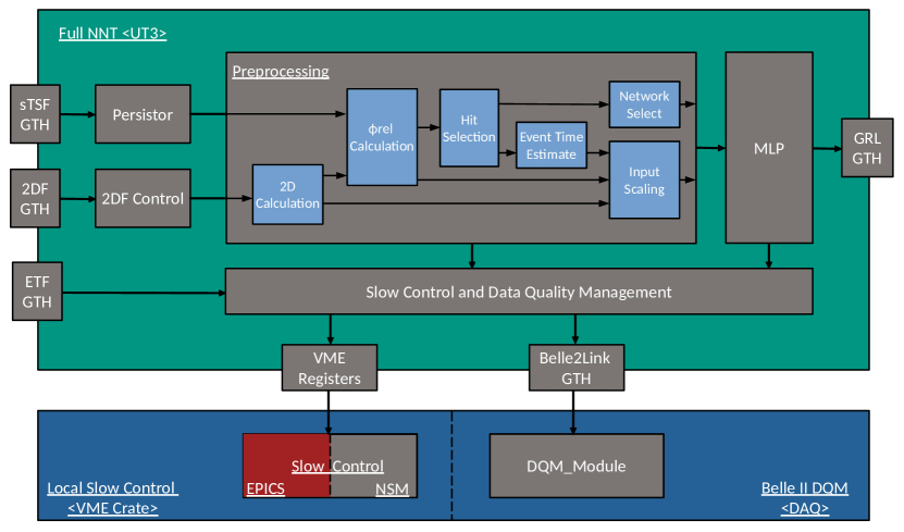
Figure 6: Details of the overall architecture of the neural trigger hardware.

Preprocessing: The general structure of the preprocessing as shown in fig. 6 consists of several data paths which are executed in parallel to keep the latency low. The individual stages are internally pipelined to achieve the frequency goal. Differences in individual processing latencies are compensated by shift registers buffering intermediate results; those are not explicitly shown in the architecture. With all inputs from the TSF and 2DF the preprocessing is generating control signals which will load a specific weight set into the neural network module. In the base configuration, the weight set will be loaded depending on the presence of stereo layers with suitable TSs (experts). The scheduling of the individual operations is performed as soon as possible under the present data dependencies, with the input scaling being the common point of synchronization right before the entry to the neural network. In general, across all modules the best choice for implementation was to use SRAM instead of DSPs. Due to their location relative to the transceivers, high availability, flexible routability, together with the high demand of DSPs within the neural network, it was more economic, in terms of resources and latency, to avoid DSPs in the preprocessing steps by using tool directives instead.

Neural Network: Processing in the neural network is performed by artificial neurons. These can be implemented by combining multiply-and-accumulate operations with the chosen activation function. The remaining parameters are then the resources to be used for the operations and the schedule for individual operations. In general, the best performance can be achieved on FPGAs when using DSPs for multiplications with variable input values. As such this realization is relying on DSP units. In addition, these units are already equipped with an internal accumulator which can be used to further increase efficiency. Its usage is, however, determined by the chosen schedule. First of all the amount of operations to be scheduled, namely $(27+1)*81+(81+1)*2=2432$ operations (see fig. 4), is exceeding by far the amount of DSPs available on the FPGA in the UT3, which are limited to about $900$ units. Due to the complexity in routing, the input signals through the physical location of the DSP on the floorplan of the FPGA, it is furthermore not possible to have an architecture with 100% resource utilization. Experimental studies have shown that the FPGA architecture does not support a utilization above 65 %, considering the system clock of 127 MHz.

The strategy to overcome this, is to use multiplexing for the multiplication of inputs by deferring a subset of inputs to later clock cycles, in turn reducing the resource demand per clock cycle. The positive side effect of this is that the internal accumulator can now be used to produce partial sums without the need of additional adder logic. The question now is how to determine the factor of multiplexing, and the choice was to define it depending on the resulting resource consumption. A multiplexing factor of $5$, this means $5$ inputs are processed on one DSP unit across multiple clock cycles, yielded the desired resource consumption which in turn resulted in timing closure later on. We note here that there are several more advanced approaches to increase the efficiency of using DSPs, for example SIMD style operations with multiple inputs and weights being interleaved to make use of the 18 and 21 bit wide data ports of the units. However, the choice here was to increase the bit width to the maximum instead of increasing operational performance itself in order to achieve higher resolutions. There is, on the other hand, a trade-off here between free resources and resolution that could be further explored. The activation function (hyperbolic tangent) is realized with a LUT which includes logic to negate the result, and different resolutions to efficiently implement the function. Here we use the Dual-Port logic provided by BRAM units on the FPGA to reduce resource consumption by sharing a LUT for two artificial neurons.

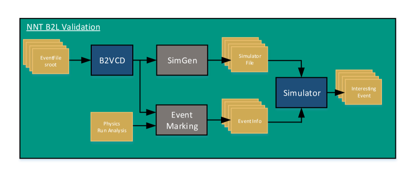
Figure 7: Process for offline verification of the hardware on clock cycle granularity.

4.3 Configuration and Testing

Verification of the hardware is based on the usage of B2Link data [18] in combination with the tool B2VCD, which is unpacking the data from specified boards and transforming integer into a VCD format which can be read by signal plotting tools such as gtkwave [19] for subsequent analysis. The file can additionally be used to generate stimuli for a cycle-by-cycle recreation of the encountered scenario in an HDL simulation tool. This is performed in the SimGen tool [20] which in addition incorporates the IO specifics of the NNT to map data onto the IO interfaces that are used at HDL-level. With this setup it is already possible to validate the runtime hardware against functional simulation to uncover problems originating from signal delays or improper interfacing. In addition to this an event-marking tool was implemented with the task to combine offline analysis which compares the hardware with ideal software execution and low-level HDL simulation. Here the idea is to identify problematic events after the run and mark down the position in the clock-by-clock simulation.

TS Depth	Persistence	$\alpha$ BW	$\phi_{rel}$ BW	Hit Selection	Multiplication
24	16	14	24	1 stage	Slices

Table 1: Architecture configuration of the preprocessing.

Weight Sets	Weight BW	Input BW	MAC	Activation	MUX
5	18	13	DSP	LUT full optimized	4

Table 2: Architecture configuration of the neural network.

Slices	Registers	DSPs	BRAM	Frequency	Latency
46%	14%	53%	49 %	127 MHz	9 data cycles / $288ns$

Table 3: Implementation characteristics for the full setup trigger.

The hardware configuration and implementation characteristics are discussed in the following. The configuration of the preprocessing is shown in Table 1, and for the neural network in Table 2. Here, TS depth is referring to the maximum amount of stereo TSs which are buffered at any clock cycle, higher depths would exceed the timing and resource budget. Persistence describes the amount of clock cycles for which a segment is buffered before being invalidated. The columns with “BW” are describing the internal bit widths for the $\alpha$ and $\varphi_{rel}$ values that are internally used, and “MAC” stands for Multiply-accumulate, “MUX” gives the multiplexing level. Table 3 is showing the resulting latency, frequency, and resource characteristics of the fully integrated trigger for the V6VHX380T FPGA on the UT3. They are fulfilling all the requirements.

5 Performance of the Neural $\mathbf{z}$-Trigger

In this section we present the performance of the $z$-Trigger , based on the data from its launch in spring 2021 until the beginning of the Long Shutdown (“LS1”) in June 2022. The $z$-Trigger was commissioned in late 2020, being monitored but not yet activated at that time. For the performance studies we will compare the neural tracks (“neuro track”) with the corresponding fully offline reconstructed tracks (“reco track”).

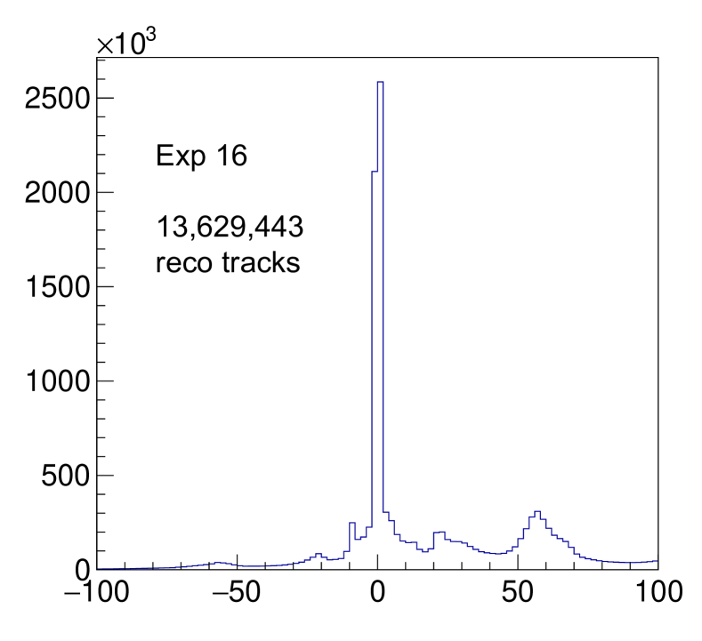
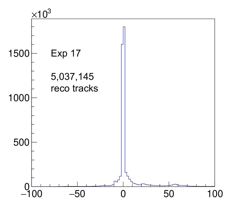
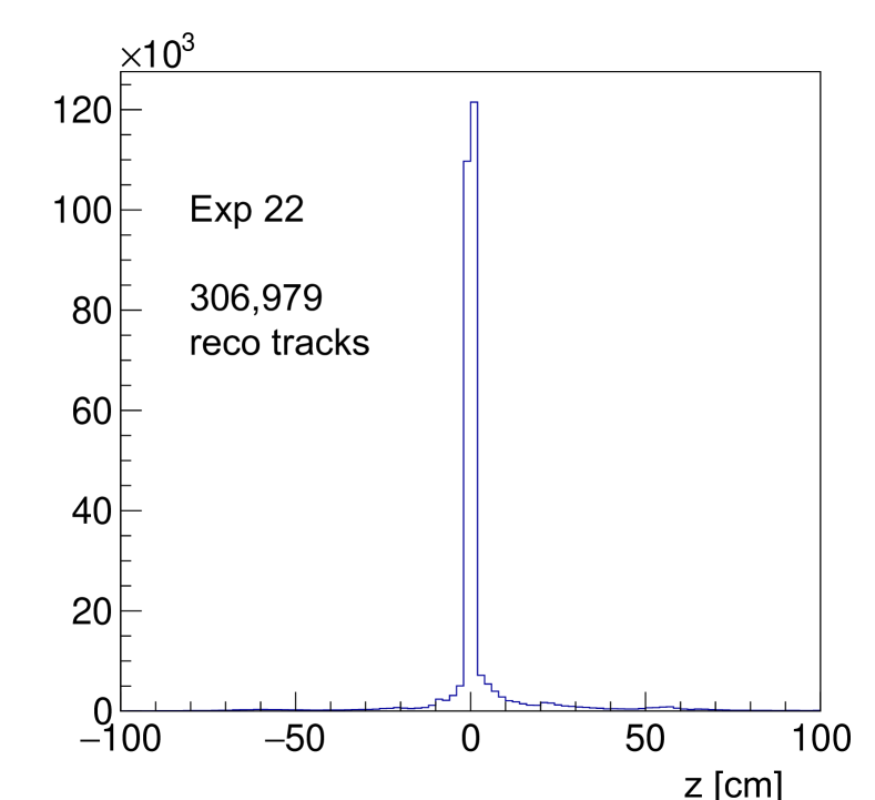
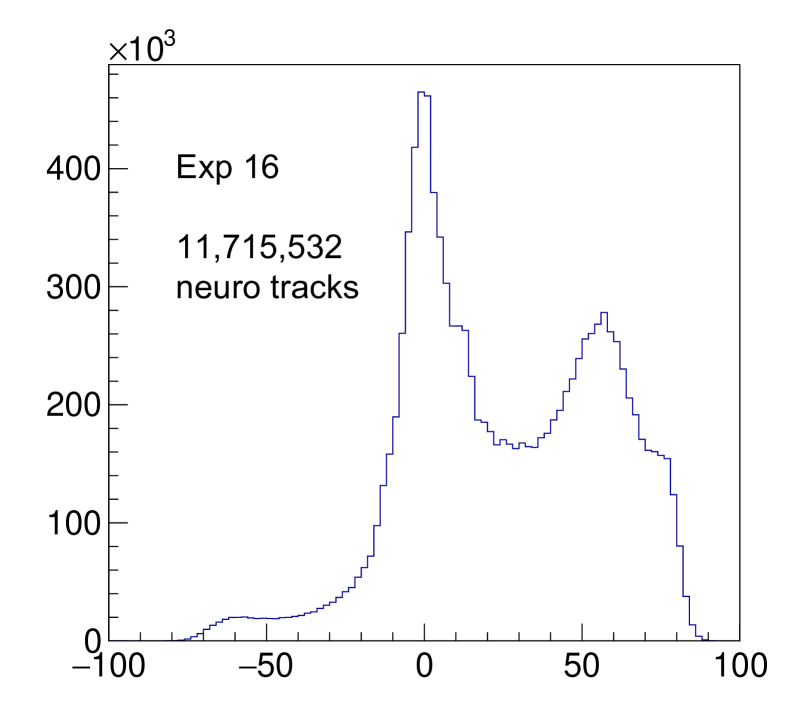
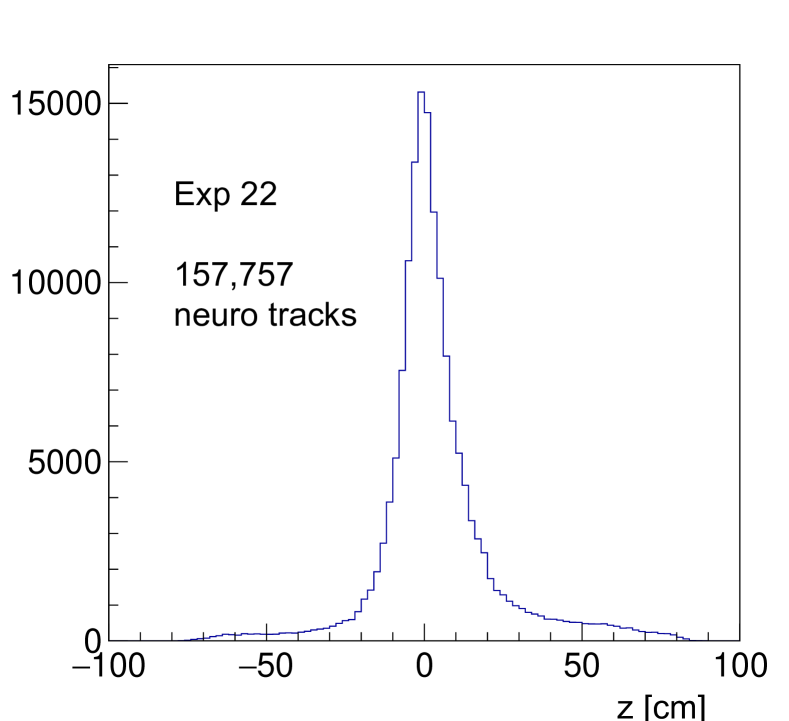
Figure 8: Left column: Distributions of fully reconstructed tracks using the offline reconstruction software package. Right column: Distributions of found neural tracks. Upper row: Exp. 16, neural $z$-trigger was not enabled. Middle row: Exp. 17 with $z$-trigger enabled for this and the following experiments. Lower row: Exp. 22 (end of 2021 running). In this latter period the machine background was significantly reduced (see text).

The most important characteristics of the neural approach is the achieved resolution in the $z$-impact of the track, as this quantity is subject to cuts in the GRL for the event acceptance at L1. Before going into the details of a $z$-dependent resolution for the neuro tracks, we show in fig. 8 distributions of the track $z$-vertex along the beam axis for reco events (left column) and the tracks found by the neural trigger hardware (right column). The three rows correspond to different experiment numbers, i.e. Exp. 16 (top row), Exp. 17 (middle row) and Exp. 22 (bottom row). The data come from special data streams written to tape, sampling all L1 triggers over the entire experiments. Typical running periods for these experiments is of order a month or more. The different experiments are characterized, for example, by special settings of the machine parameters and by certain combinations in the trigger menus. All results from the $z$-Trigger (right column of fig. 8) have been obtained from networks with the initial FANN training. No selection of events or tracks has been made, neither in the reco tracks nor in the neuro tracks found at L1. As can be seen from the figures, the number of neuro tracks is smaller compared to the number of reco tracks. This is expected due to the limited polar angle acceptance for the neuro tracks, and the limitation of tracks in transverse momentum to pass the required minimum of four of the five axial wire planes. Furthermore, some reco tracks are reconstructed offline solely in the vertex detectors, with a minimum of CDC wire planes, insufficient to set a wire trigger. Such reco tracks typically correspond to charged particles with very shallow polar emission angle or very low transverse momentum. Concerning the $z$-resolution of the neuro tracks, a first look at the peak at $z=0$ shows a resolution definitely better than 10 cm, demonstrating the readiness of the $z$-Trigger for background rejection from outside of IP.

In fig. 8 one observes a clear difference in the fraction of tracks coming from regions outside of the interaction point (IP): In Exp. 16, in the beginning of the luminosity runs of the year 2021, the neural trigger was not yet activated. The charged particles were triggered by the standard 2D system, and the machine background was quite large compared to the running in 2020. Since the total trigger rate was close to the DAQ limit at that time (spring 2021), the $z$-Trigger was switched to active in Exp. 17, requiring a $z$-cut of 20 cm for all track triggers. The result was an impressive suppression of track triggers outside the IP (see right plot in the middle row), reducing the track trigger rate by roughly a factor of 2.

During the fall of 2021 the instantaneous luminosity was steadily increased, accompanied by a strong increase of background. With the beam currents raised above 1000 mA (800 mA) for the positrons (electrons), the luminosity had reached a new record of $3.8\times 10^{34}$ cm^-2s^-1. However, there were also some shorter run periods where the background conditions for the trigger were less severe. As an example, the data from the end of the data taking (December 2021) is shown in the last row of fig. 8. Here one observes a reduced contribution from large $z$, caused by the favorable background conditions in the SuperKEKB accelerator.

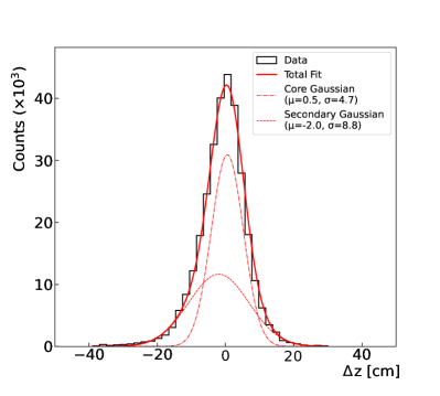
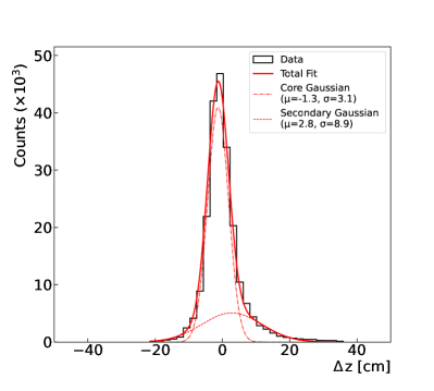
Figure 9: Difference of the $z$-positions between the reco track and the associated neuro track, in [cm], for Exp. 16 (initial FANN training) and Exp. 24 (presently used Pytorch training). The distributions are fitted with double Gaussians (see text).

Despite the short periods of “low” background before the break for the Long Shutdown (LS1) in June 2022, it became clear that the neural trigger should learn to cope with increasing beam currents and backgrounds while the machine is struggling to increase the luminosity. For this, a new training with tracks from the high background runs of 2021 was launched, using PyTorch. After optimizing the hyper-parameters in the learning process a significant improvement of the $z$-resolution was observed. Figure 9 shows, for offline reconstructed tracks from Exp. 16 (FANN) and Exp. 24 (PyTorch), the difference in $\Delta z=z_{\rm neuro}-z_{\rm reco}$ between the reco track and the corresponding neuro track. Here, events with a single reco track within the CDC acceptance (transverse momentum $p_{T}>250$ MeV, $-0.54<\cos(\theta)<0.82$) were required. The CDC conditions are necessary to make sure that tracks in the $r\phi$ plane can be found by the conventional 2D tracker, which is the required input to the preprocessing steps for the neuro tracks (see the hardware section above). In addition, a cut in the $z$-vertex of the reco track of $|z_{\rm reco}|<1$ cm was imposed to make sure that only $e^{+}e^{-}$collision events enter the sample. The distributions are described by double-Gaussians. While the initial training with FANN showed a resolution in the core Gaussian of 4.7 cm, the new training yielded a significantly better value of 3.1 cm. The wide Gaussians (dashed lines in fig. 9) with typical contributions of order 10%, have widths around 8.8 cm. Based on the improved resolution of the $z$-impact, a reduced cut of $|z|<15$ cm was chosen in the GRL for a neuro track to pass an $e^{+}e^{-}$collision event.

As explained earlier, the system of neural networks delivering $z$ and $\theta$ for the tracks in an event consists of a total of five expert networks. While the expert net “0“ is used for “clean” neuro tracks, where all 4 SLs are present, the other experts (“1 - 4”) are chosen depending on which one of the stereo layers is missing. The cooperation of the expert networks is illustrated in fig. 10. On the left column of the figure the distributions of the azimuth angle $\phi$ (top) and $\Delta z$ (bottom) for the expert net 0 are shown, on the right column the corresponding distributions for the experts 1-4. The data are taken from Exp. 24, only reconstructed tracks from the origin ($|z|<1$ cm) are selected. One observes two region of inefficiencies in the $\phi$ distribution for the expert 0. These holes are caused by local inefficiencies of the stereo drift wires during the data taking period of Exp. 24. These areas of inefficiencies are nicely “filled” by the experts 1-4 so that the combined $\phi$ distribution shows the expected uniform shape. It should be mentioned that a major portion of the inefficient regions of the CDC, caused by malfunctioning front end electronics, have meanwhile been fixed during a scheduled maintenance shutdown.

The bottom row of fig. 10 shows the $z$-resolution for clean tracks (left) compared to their complement on the right. The fraction of the clean tracks is typically around 70-80%. The $z$-resolutions are fitted by double-Gaussian functions. The resolutions of the core Gaussians are 2.8 cm for the clean tracks, and 3.8 cm for all the other tracks. This increase is understandable in view of the fact that fewer stereo SLs are available for the $z$-estimate. In particular the tracks from the “Expert 4” network have worse resolutions where the innermost stereo layer. i.e. the one closest to the track origin, is missing. A typical share between the expert networks, reflecting the inefficient regions in the CDC front end electronics before LS1, is 86% for Expert 0 and 2% each for the “inner ” Expert networks 2, 3, and 4. When the outer stereo TS is missing (Expert 1, typically 5-8 %), then the reason is a combination of CDC inefficiencies and shallow polar angles of the tracks, missing the full angular acceptance of the CDC.

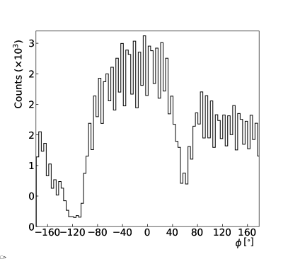
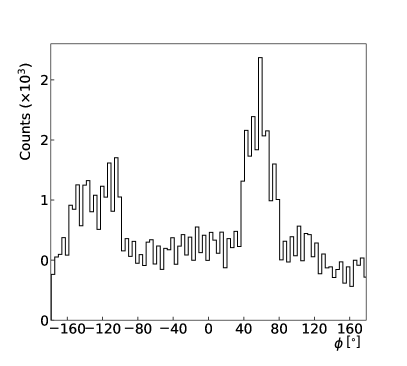
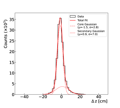
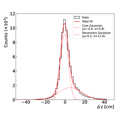
Figure 10: Distributions of the azimuth angle $\phi$ and $\Delta z$ for the neuro tracks for different numbers stereo SLs. Left column: neuro tracks with all 4 SLs. right column: neuro tracks with one of the stereo SLs missing. Data from early 2022 running (Exp. 24).

Single Track Trigger (STT):

In addition to the requirement of a neural track for all standard $\geq 2$-track triggers, it was possible to launch a minimum bias single track trigger, requiring $|z|<15$ cm, supplemented by an additional minimal requirement for the track momentum of $p>0.7$ GeV. The latter cut is necessary to suppress a large “background” coming from IP: Figure 11 shows the track momentum $p$ versus the track origin $z$ in all events after full reconstruction. The large peak around $z=0$ at low momenta comes mainly from the QED reaction $e^{+}e^{-}$$\rightarrow$ $e^{+}e^{-}$$e^{+}e^{-}$, where the secondary electrons and positrons peak at extremely low energies. The momentum cut largely reduces the QED background, but also strongly reduces the off-IP background generated by spallation protons, with typical momenta of 500 MeV.

Figure 11: Distribution of the track momentum versus the origin in $z$ for all tracks fully reconstructed in the event. A cut at 0.7 GeV (red line) gets rid of QED and also of most of the tracks from outside the IP.

At the trigger level, the momentum of the neural track is calculated from the curvature $\omega$ of the input 2D track, the known solenoid field $B$ of Belle II , and the polar scattering angle $\theta$, estimated by the network (second output of the networks, see fig. 4):

$$p[\rm{GeV}]={{1}\over{\omega[1/\rm{m}]\;\sin(\theta)}\;0.3\;\it{B}[\rm{T}]}.$$

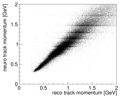
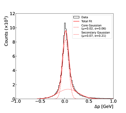
Figure 12: Left: Correlation of the true track momentum from reconstructed tracks and the momentum estimated for the neural tracks. Right: Difference of track momenta (see text).

Based on this expression the momentum of a neuro track is determined in the GRL using a look-up table for the trigonometric function $\sin(\theta)$. The momentum resolution of the neuro tracks is shown fig. 12. On the left side the correlation between the true momentum (after full offline reconstruction) with the result for the corresponding neuro track, based on the above expression. The horizontal stripes are due to the integerized hardware representation of the 2D track candidates. The tracks selected are from events triggered by the STT towards the end of the running before LS1, which was plagued by very high backgrounds (“Exp. 26”). On the right side of the figure the difference of the true and neural momentum is displayed. A fit to the distribution with a double Gaussian yields a standard deviation of about 60 MeV for the core Gaussian. As can be seen from the correlation plot, the core Gaussian mainly describes the resolution of momenta below 1 GeV.

The STT was launched as physics trigger (unprescaled) for low multiplicity events since the beginning of the year 2021. Its contribution to the total trigger rate was observed at the level of roughly 20%, which is very reasonable for a minimum bias trigger. Since only a single track is required, further tracks have no limitation set by the acceptance of the CDC. Therefore also 2-track events are triggered where the second track is only going through a few planes of the CDC and the offline reconstruction is mainly done by the vertex detectors. A comparison of the largely improved efficiency of the STT relative to the other multi-track triggers (still requiring a neural track, see above) is shown in fig. 13 for the reaction $e^{+}e^{-}$$\rightarrow\mu^{+}\mu^{-}(\gamma)$. The plot shows the efficiency as a function of the track with the smaller transverse momentum. The observed improvement of the efficiency for momenta larger than 0.7 GeV is evident.

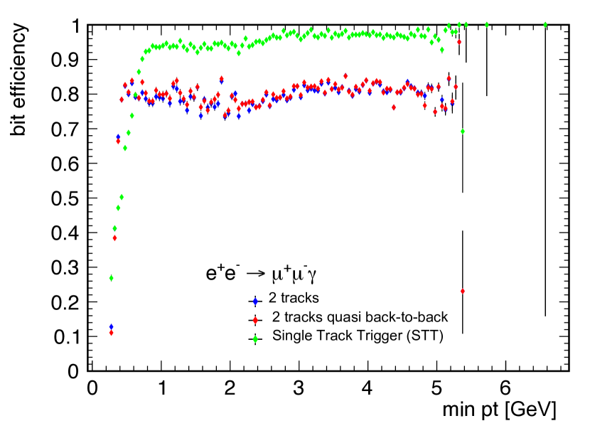
Figure 13: Efficiency of STT in comparison to the two-track triggers for the reaction $e^{+}e^{-}$$\rightarrow\mu^{+}\mu^{-}(\gamma)$, as function of the smaller transverse momentum of the two tracks.

Belle II has successfully taken physics data with the neural L1 trigger, running now at world record luminosity exceeding $4\times 10^{34}$ cm^-2s^-1. SuperKEKB aims to eventually provide instantaneous luminosities beyond ${\cal L}=6\times 10^{35}\,\mathrm{cm}^{-2}\,\mathrm{s}^{-1}$. The pure physics rate at this super-high luminosity is expected around 10 kHz, with a limitation of the maximal data logging rate of 30 kHz. This means that the L1 triggers have to be selective enough to accept a background over signal fraction of only 2 to 1, a condition for both the calorimeter and track triggers.

Towards the end of the data taking period, before the Long Shutdown LS1 in June 2022, the machine conditions for these runs (Exp. 26) were characterized by extremely large background, which led to increased rates for the $z$-Trigger , dominated by the STT: Instead of the usual 20% share in the total trigger budget, this share has increased to about 50%. On the other hand, the $z$- and $p$-resolutions for the vertex tracks did not change significantly, since the network have been retrained using data with the increased background.

Given the stable $z$-resolution of the neural trigger together with the increased rate share during periods of large background points to the fact that the $z$-resolution for the neuro tracks deteriorates with increasing displacement from IP. This is in part understandable since a relatively small fraction of tracks at $z$-values further away from IP exist for the training of the networks, after the $z$-Trigger had been enabled (see, for example, last row in fig. 8). Another “irreducible” component comes from the fact that the tracks at larger $z$ tend to have smaller polar emission angles in order to traverse sufficient SLs of the CDC. The effect of the reduced $z$-resolution for larger values of $z$ can be seen in fig. 14. In this $z$-correlation plot between reco and neuro tracks one observes “feed-down” of the real tracks with large $z$-values into the $z$-acceptance interval of the neuro tracks. These additional neuro tracks, increasing the L1 track trigger rate, are clearly visible in the horizontal acceptance band for neuro tracks at $\pm$ 15 cm. In addition, fake neural tracks are produced, mainly by an increasing rate of 2D input track candidates, formed largely by random background hits. These fake 2D tracks have a fair chance to be combined with stereo track segments also originating from background sources. Our ongoing studies to improve the $z$-resolution for the entire $z$ region ($\pm 100$ cm) with the aim to significantly reduce the feed-down and fake tracks effects is the subject of the next section.

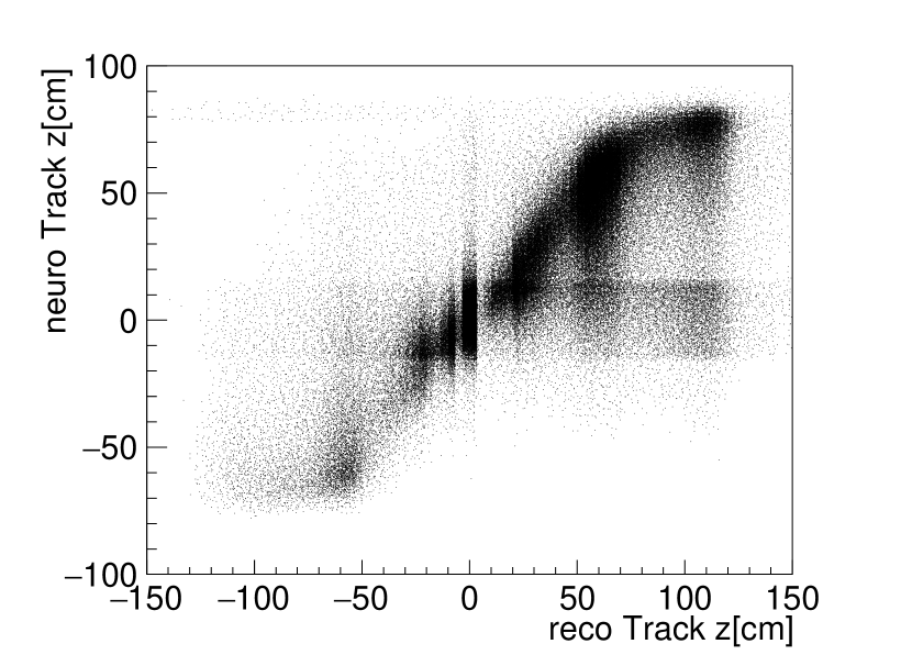
Figure 14: Correlation of the $z$-impact between the fully reconstructed tracks and the corresponding neuro tracks. The horizontal band at $\pm$ 15 cm is the single track trigger acceptance and originates from the already active STT trigger line during data taking. The “feed-down” effect into this band, mainly from the $z$ interval $\pm$ 50 cm, is clearly visible.

6 Ongoing Developments

We envisage several ways to stabilize the STT and the multi-track $z$-Trigger for future running (clearly, we exclude the possibility to simply down-scale the STT and lose physics). Since new and more powerful custom-made trigger boards (“UT4”, equipped with Virtex UltraScale 7 XCVU080/160 FPGAs) have been added recently to the L1 system, more resources are now available to overcome the limitations of the presently installed UT3 trigger boards. This means that the neural network architecture of the $z$-Trigger , limited at the moment to one hidden layer with 81 nodes only, can now be extended to a deep-learning network model, having typically 3 hidden layers with $\cal{O}$(100) nodes each. Furthermore, the track segment finders (aTSF and sTFS, see fig. 5 above) will also provide information on all other wires within TS in addition to the priority wire, although with somewhat reduced precision in the drift times (32 ns instead of 2 ns). Adding the information from additional wires within a TS, it is likely to gain better performance due to the additional constraints. This entails, of course, to widen, possibly substantially, the input layer. Preliminary studies, using additional inputs and a deep-learning architecture for the neural networks, have shown that the $z$-resolution of the vertex tracks can be further improved, and the feed-down effect can be substantially suppressed.

Most importantly, the input track candidates to the networks need to be made robust against background. Presently the track finding is carried out by the standard 2D trigger, using Hough transforms in the azimuth angles $\phi$ and the track curvature $1/r$, where at least 4 out of the 5 axial layers are required for a valid candidate. To reduce the chance of track candidates formed by background TSs, it was proposed [21] to use also the priority wires of the stereo TSs. In this scheme the 2D Hough plane is enlarged to a three dimensional Hough space, adding as third dimension the polar track angle $\theta$. The enlarged Hough space has the advantage that now all nine SLs (instead of only the 5 axial SLs at present) can be used for track finding, making random noise much less likely. As a further advantage of the 3D Hough space the track candidates are forced to come from IP, thus naturally suppressing tracks from outside.

As powerful tool to reject background hits and fake tracks the 3D Hough method uses an optimized cluster algorithm beyond simple peak finding. The contents of the Hough cells relative to the cluster maximum define a set of cluster shape variables which can be used to discriminate clusters from real tracks against those from random noise. Recent studies have shown that even under very severe background conditions, extrapolated to the design luminosity, the 3D Hough model finds the correct tracks with high efficiency and at the same time strongly reduces the fake candidates. In a future step we may also consider using all the wires in the track segments and do the track finding in the 3D Hough space with all wires. We have found that the 3D Hough method, analyzed in terms of the optimized cluster algorithm with a static neighborhood around the maximum can be realized in the new UT4, leaving enough resources for enlarged input layers and deep-learning network architectures.

There are also studies going on to implement a neural trigger, working in parallel to the $z$-Trigger , to identify track pairs with a strongly displaced vertex (“Displaced Vertex Trigger” DVT). Such event signatures are expected, for example, in models that predict inelastic dark matter production in association with a dark Higgs boson [22]. The method of choice for the track finding at L1, given the wire preprocessing blocks up to and including the track segment finders (see fig. 5), is the 2D Hough transform again. Here, however, a vertex hypothesis is necessary to create the intersecting curves in the Hough space. For the $e^{+}e^{-}$collision events the case is clear: the vertex is the IP, well approximated by $(x=0,y=0)$. For the displaced vertices, however, the origin is unknown. The method of choice is to put a grid of possible vertex locations (we call them “macro cells”) over the transverse cross section of the CDC. A typical number of the finite-size macro cells is of order 100, where the Hough transforms have to be executed with each of these macro cells as vertex hypothesis. But then it turns out that simple peek finding in the Hough space will not be selective enough to pin down the correct macro cell. The solution found here is to employ neural networks to analyze the Hough cluster shape, similar to the way described above for the 3D track model. In the new UT4, the parallel execution of all Hough transforms seems possible within the latency attributed to the L1 track trigger.

7 Conclusions and Outlook

For the Belle II experiment, running at the SuperKEKB asymmetric-energy electron-positron collider, the first L1 track trigger world-wide based on neural networks has been realized. The neural trigger uses the information of the axial and stereo wires of the Central Drift Chamber (CDC). The input to the networks are the track candidates provided by the standard Belle II track trigger, which are found by means of Hough transforms using the axial wires only. This 2D trigger is unable to reject the overwhelming track rate generated by beam collisions with the beam pipe and structures of the beam focussing system. With these 2D track candidates as input, adding the stereo wires of the CDC, a set of single hidden layer networks provide as outputs the vertex of the tracks along the beam ($z$)-direction and the polar emission angle $\theta$. With this information the neural trigger rejects events coming from outside of the electron-positron interaction point ($z=0$). This rate is so large that all track triggers have to require at least one neural track with the condition $|z|<15$ cm.

Using the polar angle $\theta$ it is even possible to deploy an unprescaled, minimum-bias single track trigger (STT), which requires a mild momentum cut of 0.7 GeV in addition to the acceptance cut of $|z|<15$ cm. Although the STT has boosted the track trigger efficiency, especially for low charged-multiplicity final states, it showed some sensitivity to the strongly increasing backgrounds with the machine’s program to raise the luminosity towards design values. While the performance of the STT for physics triggers was not affected by the high backgrounds, demonstrating the robustness of the neural approach, it showed an over-proportional increase in trigger rate, generated mainly by the background-prone 2D track finding algorithm. In order to provide stable operation for the STT also in the future, a comprehensive upgrade program is in progress, mainly replacing the traditional 2D track finding by a novel three-dimensional Hough space analysis, and an extension of the network structure to a deep-learning architecture with additional wire inputs.

Since the neural triggers so far are optimized for tracks coming from the interaction point, they will miss event signatures with tracks coming from a strongly displaced vertex. Such event signatures are expected in various extensions of the standard model that predict long-lived particles. We have concrete plans for the near future to add neural algorithms to the Belle II L1 track trigger system for such anomalous event types.

The hardware level neural network track trigger developed for the Belle II experiment and described in this paper represents a significant step towards fast and intelligent data collection and processing methodologies in scientific research. The innovative approach to integrate machine learning techniques into the hardware of the experiment indicates the possibility for a paradigm shift towards embracing smarter and faster solutions for real-time event selection. It also sets a precedent for future experiments where efficient and accurate data collection as well as extraction of novel features are essential.

References

- [1]
- [2] T. Abe et al., Belle II Technical Design Report, KEK-REPORT-2010-1, arXiv:1011.0352v1 [physics.ins-det] (2010).
- [3] S. Hashimoto et al., LoI for KEK Super B Factory, Part I: Machine, KEK-Report 2004-4 (2004).
- [4] KEKB B-Factory Design Report, KEK Report 95-7, August 1995.
- [5] Belle Collaboration, A. Abashian et al., The Belle detector, Nucl. Instr. Meth. Phys. Res. A 479 (2002) 117.
- [6] C. Bernardini et al., Lifetime and beam size in a Storage Ring, Phys. Rev. Lett. 10 (1963) 407.
- [7] A. Piwinski, The Touschek Effect in Strong Focusing Storage Rings, arXiv:physics/9903034v1 [physics.acc-ph] (1998).
- [8] J. H. Köhne, C. Kiesling et al., Realization of a Second Level Neural Network Trigger for the H1 Experiment at HERA, Nucl. Inst. Meth. Phys. Res. A 389 (1997) 128.
- [9] Hough, P.V.C. “Method and means for recognizing complex patterns”, U.S. Patent 3,069,654, Dec. 18, 1962; Duda, R.O.; Hart, P. E. (January 1972). ”Use of the Hough Transformation to Detect Lines and Curves in Pictures”. Comm. ACM. 15: 11–15, Jan. 1972.
- [10] S. Skambraks, Use of Neural Networks for Triggering in Particle Physics, Diploma Thesis, Ludwig-Maximilians-Universität München, 2013.
- [11] F. Abudinén, Studies on the neural -Vertex-Trigger for the Belle II Particle Detector, Master Thesis, Ludwig-Maximilians-Universität München, 2014.
- [12] S. Pohl, Track Reconstruction at the First Level Trigger of the Belle II Experiment, PhD Thesis, Ludwig-Maximilians-Universität München, 2018.
- [13] B. Abi et al., Muon g-2 Collaboration, Phys. Rev. Lett. 126, 141801 (2021).
- [14] Belle II collaboration, Belle II Analysis Software Framework (basf2),458 https://doi.org/10.5281/zenodo.5574115. doi: 10.5281/zenodo.5574115.
- [15] A. Paszke, S. Gross et al., PyTorch: An Imperative Style, High-Performance Deep Learning Library, Advances in Neural Information Processing Systems 32 (2019).
- [16] D. P. Kingma and J. Ba, Adam: A Method for Stochastic Optimization, 3rd International Conference for Learning Representations, San Diego (2015)
- [17] S. Bähr, Implementation of a Neural Network Trigger for Belle II on FPGA, PhD Thesis, Karlsruhe Institute of Technology, 2020.
- [18] Denhui Sun, Zhen’an Lium,Jingzhou Zhao, and Hao Xu, Belle2Link: A Global Data Readout and Transmission for Belle II Experiment at KEK, Physics Procedia, Volume 37, 2012, Pages 1933-1939.
- [19] https://gtkwave.sourceforge.net/
- [20] Michal Pasternak, Nafiseh Kahani, Mojtaba Bagherzadeh, Juergen Dingel, and James R.Cordy, Simgen: A Tool for Generating Simulations and Visualizations of Embedded Systems on the Unity Game Engine, Proceedings of the 21st ACM/IEEE International Conference on Model Driven Engineering Languages and Systems: Companion Proceedings (2018), isbn = 978-1-4503-5965-8, Copenhagen, Denmark, p. 42-46.
- [21] S. Skambraks, Efficient Physics Signal Selectors for the First Trigger Level of the Belle II Experiment based on Machine Learning, PhD Thesis, Ludwig-Maximilians-Universität München, 2020.
- [22] see, e.g., David Smith and Neal Weiner. Inelastic dark matter. Physical Review D, 64(4), 2001; Duerr, M., Ferber, T., Garcia-Cely, C. et al. Long-lived dark Higgs and inelastic dark matter at Belle II. J. High Energ. Phys. 2021, 146 (2021). https://doi.org/10.1007/JHEP04(2021)146.