Reinforcement Learning with Elastic Time Steps

Abstract

Traditional Reinforcement Learning (RL) algorithms are usually applied in robotics to learn controllers that act with a fixed control rate. Given the discrete nature of RL algorithms, they are oblivious to the effects of the choice of control rate: finding the correct control rate can be difficult and mistakes often result in excessive use of computing resources or even lack of convergence.

We propose Soft Elastic Actor-Critic (SEAC), a novel off-policy actor-critic algorithm to address this issue. SEAC implements elastic time steps, time steps with a known, variable duration, which allow the agent to change its control frequency to adapt to the situation. In practice, SEAC applies control only when necessary, minimizing computational resources and data usage.

We evaluate SEAC’s capabilities in simulation in a Newtonian kinematics maze navigation task and on a 3D racing video game, Trackmania. SEAC outperforms the SAC baseline in terms of energy efficiency and overall time management, and most importantly without the need to identify a control frequency for the learned controller. SEAC demonstrated faster and more stable training speeds than SAC, especially at control rates where SAC struggled to converge.

We also compared SEAC with a similar approach, the Continuous-Time Continuous-Options (CTCO) model, and SEAC resulted in better task performance. These findings highlight the potential of SEAC for practical, real-world RL applications in robotics.

I Introduction

Model-free deep reinforcement learning (RL) algorithms have demonstrated their versatility in diverse areas, ranging from gaming [1, 2] to robotic control [3, 4]. Integrating RL with high-capacity function approximators, such as neural networks, promises to automate decision-making and control tasks. Despite their potential, a significant barrier to their broader real-world application remains. Standard practice involves transferring data from RL simulations to real-world applications at a high, fixed control rate. While effective in many scenarios [4, 5], our prior research [6, 7] is the first one to highlight a critical limitation of this approach: the risk of generating ineffective controls under the fixed rate assumption.

Consider the example of driving a car in a large, obstacle-free environment: minimal control actions are necessary. In contrast, navigating tight spaces or following complex paths demands a higher control rate. Setting a fixed control rate necessitates choosing a rate that accounts for the worst-case scenario, an average rate if safety is less critical to ensure the system’s controllability.

Furthermore, control rate is critical in continuous control systems, impacting more than just computational load. In designs influenced by physical properties, like inertia, the timing of actions is crucial. Take a car driving on a road as an example. The outcomes are vastly different if we apply the same force of 100 Newtons for different durations, say 1 second versus 0.1 seconds. Amin et al. and Park et al. found that with a higher control rate, the RL model can perform worse than the lower control rate RL model [8, 9].

However, low frequency will rapidly reduce the flexibility of the entire control strategy, making this strategy unsuitable for handling some complexed scenarios. For example, Yann et al. thought a high control rate was necessary for the RL model to deploy in the delayed environment [10]. These studies highlight that the success of continuous control reinforcement learning models largely depends on the control rate. However, there’s no one-size-fits-all approach: whether a higher or lower control rate is better varies based on which environment the model is used. This means a single, unchanging control rate might not lead to the best outcomes in continuous control reinforcement learning.

In this paper, our research shows how a fixed control rate can affect the performance of the Soft Actor-Critic (SAC) algorithm [11, 3]. Using the wrong control rate can significantly hinder the SAC algorithm’s ability to converge or find optimal solutions. This finding is crucial because it suggests elastic time steps can be necessary for effective reinforcement learning in real-world applications.

The research community’s investigation into the influence of control frequency on reinforcement learning is developing. Amirmohammad Karimi et al. conducted research shortly after ours, focusing on the impact of control rate on RL [12]. They found that a high control rate could detrimentally affect RL performance in specific scenarios. However, their Continuous-Time Continuous-Options (CTCO) model initially did not adequately consider the minimum execution time for each action. This oversight led to a system where the execution time for a step could be set to zero, a notable theoretical shortcoming. Any intelligent agent must have a minimum duration for action execution to ensure complete and safe operation. Without this consideration, the model’s applicability and reliability are potentially compromised.

Furthermore, their research did not adequately address the impact of varying control rates on task completion time. In environments with variable control rates, reducing the number of steps doesn’t necessarily correlate with minimizing completion time. This can lead to substantial variations in task completion times, which is impractical for real-world use. For instance, a control model where task completion time ranges from 1 minute to 1 hour would be too unpredictable for many practical applications. This unpredictability could hinder the efficacy of the model in real-world settings.

Sharma et al. [13] introduced the concept of learning to repeat actions, a theoretical contribution in this field. Building on this idea, Metelli [14], Lee [15], et al. applied it to solve some applications. Their work demonstrated How to achieve effects similar to a dynamic control rate using a fixed control rate through repeated actions. However, it’s important to note that this approach doesn’t necessarily reduce computational demands. This distinction is crucial, especially when considering actions executed at different frequencies, which can vary the computational load significantly. Such considerations are vital for deploying these models in practical settings, particularly robotics, where computing resources may be limited. We believe that, at least in continuous control reinforcement learning, the control rate issue deserves sufficient attention from the community.

Our prior work introduced Reinforcement Learning with Elastic Time step and developed a unique reward policy that calculates energy and time loss. This policy was implemented into the Soft Actor-Critic (SAC) algorithm, creating the Soft Elastic Actor-Critic (SEAC). SEAC is a variable time step reinforcement learning algorithm aiming to minimize the compute energy cost and the time to finish a task. In the third section of that paper, we detailed the configuration of our reward policy and the difference with Hierarchical reinforcement learning (HRL) [16]. We eliminated the unnecessary elements of HRL, simplifying our approach and making it more adaptable. We discussed strategies for optimizing the total reward by balancing the number of time steps with overall time efficiency. The fourth section explained modifications to the network structure, enabling the actor-network to predict only positive times. This was then contrasted with the network structure of the standard SAC implementation. However, our validation of SEAC was limited to an essential Newtonian Kinematics movement environment in that paper, primarily due to fewer gym environments supporting the change of control rate. Success in this simplified context doesn’t automatically imply that our method applies to more complex real-world scenarios. Moreover, we lacked a comparative analysis of reinforcement learning algorithm performances across different fixed control rates. As such, further research is needed to conclusively demonstrate the robustness and superiority of our elastic time steps method in various applications.

In this paper, we designed a set of two maze environments based on Newtonian kinematics, verified the performance of SEAC based on these environments, and compared it with the performance of the SAC algorithm at different fixed frequencies. Our results show that SEAC is superior to some fixed-frequency SAC algorithms in terms of training speed and stability, verifying SEAC’s high data efficiency and robustness. At the same time, we also compared the results of SEAC with the results of the Continuous-Time Continuous-Options (CTCO) algorithm proposed by Amirmohammad Karimi et al. In addition, we also used SEAC to challenge the competition performance of Ubisoft TrackMania 2023 [17] and compared its results with those of the SAC algorithm.

This paper primarily validates the robustness and data efficiency of the Soft Elastic Actor-Critic (SEAC) algorithm. And compared with the performance of CTCO, the only variable control rate reinforcement learning algorithm in the community except for our SEAC. The key contributions are as follows:

1. Enhance Data Efficiency: SEAC significantly reduces computational load by dynamically adjusting the control rate, improving data efficiency;

2. Stable Performance and Faster Training: Compared to fixed-frequency model-free algorithms like the SAC algorithm, SEAC demonstrates a more stable convergence capability. Additionally, in some fixed-frequency scenarios where SAC is used, SEAC achieves faster training speeds. Compared to CTCO, SEAC performs similarly in training speed and energy consumption but offers superior and more consistent results regarding time efficiency;

3. Capability in Complex Scenarios: In complex tasks, such as Ubisoft Trackmania 2023, SEAC outperforms SAC by completing challenges in fewer steps and less time.

The rest of the paper is organized as follows. Section II offers a literature review and background. Section III describes our test environments, including the Newtonian Kinematics Maze and Ubisoft Trackmania 2023. In Section IV, we detail SEAC’s structure and settings. Section V reports on simulation parameters and results. The paper concludes in Section VI.

II Related Work

Model-free reinforcement learning (RL) has shown significant success in areas like gaming and control. A standout example is Sony’s development of autonomous racing cars. This approach has enabled their AI racers to surpass human performance, achieving remarkable results as reported by Wurman et al. [4]. Their method employed a fixed training frequency of 60 Hz. However, it’s crucial to recognize that success does not always imply optimality. As mentioned in Section I, fixed control rates often lead to numerous ineffective controls. An optimal control strategy would minimize these invalid controls, adapting the duration of action steps to the evolving demands of the task rather than adhering to a rigid frequency.

In our recent work, we propose a novel reward policy that predicts not only the value of an action but also its duration [7]. This setting allows agents to choose actions at variable frequencies, a method more suited to physical systems that don’t require a constant control rate. This approach trains the policy to determine the timing and the action simultaneously, thereby adapting dynamically to changing demands. The aim is to manage environmental uncertainties efficiently and conserve the agent’s computational resources.

Similar to our work, Amir Mohammad Karimi and colleagues have developed the Continuous-Time Continuous-Options (CTCO) framework for reinforcement learning (RL) [12]. CTCO’s effectiveness is shown in simulations and a real-world task with a robotic arm. However, as previously noted, they did not realize how significant frequency changes affect the time it takes to complete a task.

Sharma et al. [13] introduced learning to repeat, a method to convert fixed ”expanded” frequencies into variable frequencies. Their strategy involves repeating the same action with consistent execution time to vary the action duration effectively. However, this method falls short in real-world applications. For instance, repeatedly executing a 1-second action ten times and a single 10-second action once have vastly different computational demands, which Sharma et al.’s method is unconcerned with.

Other works that have applied repetitive behaviors in real-world scenarios remain scarce except for Metelli [14] and Lee [15]. We also observed that Chen et al. [18] attempted to alter the ’control rate’ by introducing actions like ’sleep,’ but this still involves fixed-frequency system status checks, which doesn’t effectively reduce computational load [9].

Time-sensitive tasks in domains like robotics and electricity markets typically use fixed control rates [19, 20, 21, 22]. This is problematic for systems with limited computational resources, such as Raspberry Pi [23] or ultrabooks, which struggle to maintain high, fixed control rates.

Our algorithm follows reactive principles [24] and effectively reduces the computational load. It is designed to be adaptable and suitable for training various continuous control reinforcement learning strategies. This includes applications from robotic control to real-time strategy games like Trackmania 2023. We have successfully applied this algorithm in this game in this paper, providing a practical example.

III Settings for SEAC Application Environments

To validate and implement SEAC, our research involves two distinct test environments, each designed to challenge different aspects of the system:

1. Maze Environment: Utilizing a maze based on Newtonian Kinematics with two distinct map sets operational in the gymnasium [25], we aim to assess SEAC’s navigational and problem-solving capabilities. These environments also allow us to explore the impact of varying control rates on a fixed control rate-based Model-free RL algorithm. The layout of these mazes and the challenges are depicted in Figure 1.

2. Trackmania 2023: Developed by Ubisoft, Trackmania 2023 is a real-time strategy racing game. This dynamic environment is ideal for testing SEAC’s strategic planning, adaptability, and real-time decision-making skills in a competitive setting. Figure 2 illustrates this testing environment.

For Maze game, the starting and ending points are randomly generated but maintained at a certain distance from each other to ensure consistent testing conditions. This randomness introduces variability in each trial, testing the agent’s adaptability and problem-solving in changing scenarios. For detailed information on each map’s physical properties and specific parameters, please refer to Table I.

For Trackmania 2023, this is a racing competition to see who can complete the entire track in less time. We employed the map developed by the TMRL team for a direct and intuitive comparison of our SEAC algorithm’s performance against their SAC algorithm, utilizing the identical track for consistency in our analysis. The TMRL team’s [2] adoption of the OpenPlanet plugin [26] was instrumental in facilitating real-time data acquisition from Trackmania 2023, resulting in the fact that the training on this game can only based on real-time. Additionally, Table III in our paper provides a detailed account of the physical characteristics of the Trackmania 2023 environment as furnished by TMRL.

By employing these diverse testing grounds, we aim to evaluate SEAC’s adaptability and performance comprehensively. Such an approach is crucial in demonstrating the potential of SEAC in varied and complex real-world scenarios, paving the way for future advancements in autonomous agent systems.

III-A Details of The Maze Game

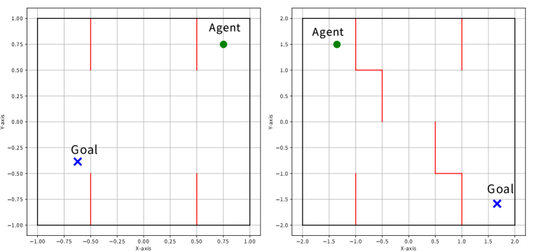
Figure 1: We have two designs for the maze maps: 1. Simple Version: The map on the left measures 2 meters in length and width. It includes four walls, with larger intervals between them. This setup is intended to test basic navigational skills under less restrictive conditions. 2. Difficult Version: In contrast, the map on the right is more extensive, measuring 4 meters in both dimensions and contains eight walls. This design restricts the agent’s movement area, presenting a more challenging navigational task.

These environments we create are a continuous two-dimensional (2D) space characterized by a starting point, a goal, and many walls. The primary objective is to navigate the agent from the start to the goal, ensuring avoidance of any wall collisions. Each reset of the environment randomly generates new start and goal locations. An episode concludes when the agent reaches the goal or collides with a wall. The agent’s movement adheres to Newton’s laws of motion, including the effects of friction.

We employ the line segment intersection judgment method to ascertain whether the agent traverses through walls, as outlined by Balaban (1995) [27]. This algorithm necessitates defining start and end points for the wall and the agent. Consequently, we define the state value that includes the positions of all walls, along with the agent’s distance to the nearest wall. We include the duration for the last time step and the force applied for the previous time step as part of the state value. The action value is the duration of the current step and the force applied in the X and Y directions. Further elaboration is provided in Definition 1 and Table I. Reward settings is in Table II.

Definition 1

The Newton Kinematics formulas are:

$$D_{aim}=1/2\cdot(V_{aim}+V_{current})\cdot T;$$ (1)

$$V_{aim}=V_{current}+AT;$$ (2)

$$F_{aim}=mA;$$ (3)

$$F_{true}=F_{aim}-f_{friction};$$ (4)

$$\begin{split}f_{friction}&=\mu mg,IfF_{aim}>f_{friction}\\ &\&V_{agent}\neq 0;\\ &=F_{aim},IfF_{aim}\leq f_{friction}\\ &\&V_{agent}=0.\end{split}$$ (5)

where $D_{aim}$ is the distance generated by the policy that the agent needs to move. $V_{agent}$ is the speed of the agent. $T$ is the time to complete the movement generated by the policy, $m$ is the mass of the agent, $\mu$ is the friction coefficient, and $g$ is the acceleration of gravity.

TABLE I: Newtonian Kinematics Maze Game Environment Details

Newtonian Kinematics Maze Game information
	Maze (simple)		Maze (Difficult)
Size	$(-1,1)$ $m$		$(-2,2)$ $m$
Min Reset Distance	$-0.15$ $m$		$0.5$ $m$
Numbers of Walls	$4$		$8$
State Dimension	$26$		$42$
Action Dimension	$3$		$3$
Maxium Speed	$2.0$ $m/s$		$2.0$ $m/s$
Weight	$20$ $Kg$		$20$ $Kg$
Static friction coeddicient ($\mu$)	$0.28$		$0.28$
Control Rate	$(1,100)$ $Hz$		$(1,100)$ $Hz$
Force	$(-100,100)$ $N$		$(-100,100)$ $N$
Gravity Factor	$9.80665$ $m/s^{2}$		$9.80665$ $m/s^{2}$

TABLE II: Reward Policy for The Newtonian Kinematics Maze Game

Reward Policy
Name	Value		Annotation
	$100.0$		Reach the goal
r	$-100.0$		Crash on walls
	$-0.1\cdot D_{goal}$		$D_{goal}$: distance to goal

III-B Details of The Racing Game

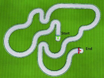
Figure 2: Comparative Analysis: SEAC vs. SAC Results on a Shared TMRL Team Designed Trackmania 2023 Map.

In Trackmania 2023, the OpenPlanet plugin captures several key features:

1. Car Speed: Tracks the real-time speed of the car.

2. Car Gear: Shows the current gear of the car’s engine.

3. Wheel RPM: Measures the wheels’ revolutions per minute.

4. RGB Image Data: Provides real-time visual data from the game.

While radar data is available, it’s not used in its setup. But we don’t use them. The SEAC navigation model is based on image data. The same as the SAC control model that the TMRL team trained.

For controlling the car in the game, Trackmania offers:

1. Gas Control: Adjusting the car’s speed in real time.

2. Brake Control: Managing the car’s braking action.

3. Yaw Control: Directing the car’s rotation around the vertical axis.

The action value includes the control rate at which these controls are applied.

The reward system in the game is designed to encourage efficient path following: more rewards are given for covering more path points in a single move. This approach is consistent with the TMRL team’s methodology [2].

Our primary objective is to enhance data efficiency and reduce the computational energy and time required to complete tasks. To ensure our comparison is valid, we maintain uniformity in several aspects: both models use the same visual-based navigation and adhere to a consistent task reward policy. The only variable we alter is the control rate. This approach allows us to isolate the impact of control rate adjustments on data efficiency.

The game is based on Newton’s kinematics, so the cars move realistically. But there’s no feature for car damage or crash detection. This means that even though the cars behave like real cars, the game’s API doesn’t provide any information about crashes. Further details are likely available in Table III, explaining the specifics of these features and their implementation in the game.

TABLE III: Trackmania Environments Details

State and action information of Trackmani
	Maze (simple)		Maze (Difficult)
State Dimension	$142$		Details in the next section
Car Speed	$(-1,1)$		Units unknown, normalized
Car Gear	$(-1,1)$		Units unknown, normalized
Wheel RPM	$(-1,1)$		Units unknown, normalized
RGB Image	$(64,64,3)$		RGB array
Action Dimension	$4$
Gas Control	$(-1,1)$		Units unknown, normalized
Break	$(-1,1)$		Units unknown, normalized
Yaw Control	$(-1,1)$		Units unknown, normalized
Control Rate	$(5,30)$ $Hz$

Our CPU’s performance limits us, preventing stable real-time control above 30 Hz. Additionally, Trackmania 2023 has a system limitation where users are logged out after a week, impacting our training process. Since our training is in real-time, we didn’t use 1 Hz as the minimum control rate. A control rate this low would overextend the training duration, risking an automatic logout by Trackmania 2023 before training completion.

IV Implementations of SEAC

In line with our previous methods, We adopt the same energy and time consumption reward policy as shown in Definition 2.

Definition 2

The reward function is defined as:

$$R=\alpha_{t}\cdot R_{t}-\alpha_{\varepsilon}\cdot R_{\varepsilon}-\alpha_{\tau}\cdot R_{\tau}$$ (6)

where
$R_{t}$ = $r$, $r$ is the value determined by task setting;
$R_{\varepsilon}=\varepsilon$, $\varepsilon$ is the energy cost of one time step;
$R_{\tau}=\tau$, $\tau$ is the time taken to execute a time step.
$\alpha_{t},\alpha_{\varepsilon},\alpha_{\tau}$ are parametric weighting factors.

We determine the optimal policy $\pi^{*}$, which maximizes the reward $R$.

When you control an agent (like a robot or software) more, it takes more steps and calculations to finish a task, but it’s usually quicker. If you control it less, it takes fewer steps and less effort, but it’s slower. The key is to find a balance so the agent works efficiently without too much or too little action. This balance is the ideal way or the ”optimal policy” for the agent to work well.

IV-A Implementations on Trackmania 2023

However, we did make some minor adjustments in the implementation for the two different environments. Unlike the maze game, all data can be input directly, and the training is based on the events, not the real-time. Trackmania 2023 demands data preprocessing, and the training progress is based on real-time. Therefore, the time provided by the policy can’t be used as the control rate for the current step, as depicted in Figure 3. So, our implementation of this game is slightly different.

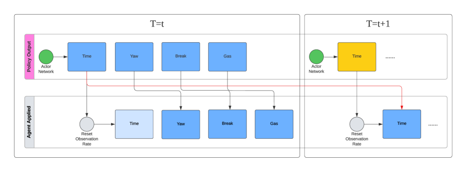
Figure 3: Trackmania 2023 operates in a delayed environment, built in rtgym [28]. Due to this delay, as highlighted by Bouteiller et al. [10], there’s a difference between the observed and actual state values. This means we first need to update the observation rate when we adjust the control rate. The updated control rate only becomes effective in the subsequent step. To adapt to this, we’ve tweaked the SEAC strategy to predict the control rate needed for the following action.

To understand the control rate’s impact on speed and acceleration, our neural network analyzes changes in sequential images. We input four consecutive images and the time intervals between them into the network. These images are first converted to grayscale and then processed through a convolutional neural networks (CNN) [29] to extract features, converting the image data from a (4, 64, 64, 3) matrix into a (128, 1, 1) matrix. Our CNN network is made up of four convolutional layers. The first layer uses a kernel size of 8 and a stride of 2. This layer processes grayscale images with dimensions (4, 64, 64) and transforms them into a matrix of size (64, 1, 1). The second layer also uses a kernel size of 4 and a stride of 2, producing an output matrix of the same size (64, 1, 1). With the same kernel size and stride, the third layer expands the output to a (128, 1, 1) matrix. Finally, using the same kernel size and stride, the fourth layer maintains the output at (128, 1, 1). Additionally, we incorporate the car’s speed, gear, and wheel RPM data from the OpenPlanet plugin. By combining these with inputs from the first two actions, we form a 142-dimensional state, which serves as the input for the actor network. The rest data details in Table III.

V Experimental Results

We conducted six experiments on SEAC, CTCO and SAC (1 Hz, 20 Hz, and 100 Hz) on two sets of maze maps, with each fixed frequency having six independent experiments on each map. We conducted experiments on SEAC on the Trackmania 2023 game for over 742.3 hours. .These experiments were conducted on a computer with CPU: I5-13600K and GPU: NVIDIA RTX 4070. The system running maze experiments is Ubuntu 20.04, and the system running the racing experiment is Windows 11. Ultimately, we chose the best-performing tests to include in our report.

V-A Results of the Maze Game

We show how well our method works clearly and intuitively by using two line graphs (Figure 4 and 5) that show average returns. Also, we draw three raincloud graphs to compare the energy and time needed by SEAC, CTCO and SAC in 1000 different tasks (Figure 6, 7 and 8). These graphs help readers understand the impact of different control rates on training convergence, the impact on energy and time costs, as well as the performance of SEAC and CTCO. To maintain a fair comparison, we trained CTCO in the same reward policy 2 environment as SEAC to evaluate their training speeds. Additionally, we trained the CTCO model in the difficult version of maze environment without our specific reward settings. This allowed us to compare the energy and time efficiency of SEAC and CTCO. It’s important to note that CTCO has not been specifically optimized for these aspects. Appendix -A provides all hyperparameter settings and implementation details.

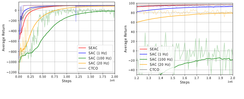
Figure 4: Average returns for SEAC, CTCO and SAC (with three control rates) trained in 2 million steps under simple verison of our maze map. The figure on the right is a partially enlarged version of the figure on the left.

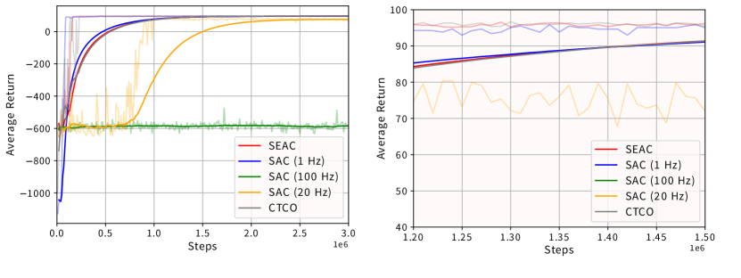
Figure 5: Average returns for SEAC, CTCO and SAC (with three control rates) trained in 3 million steps under difficult verison of our maze map. The figure on the right is a partially enlarged version of the figure on the left.

Figure 4 and 5 show that SEAC surpasses the baselines regarding average return and training speed. We observed that SEAC, CTCO and SAC (1 Hz) have similar training speeds. However, SEAC and CTCO’s ultimate average return is higher. The data presented in Figure 4 shows that CTCO trains faster than SEAC. However, Figure 5 indicates the difficult version of the maze map where SEAC’s training speed is comparable to CTCO’s. Notably, at 1.4 million steps, SEAC and CTCO simultaneously achieve average returns surpassing SAC (1 Hz). This comparison is highlighted with a specific focus on the right side of Figure 5. Based on these observations, we conclude that SEAC and CTCO’s training speeds are similar. Meanwhile, SEAC is noticeably quicker than both SAC (20 Hz) and SAC (100 Hz). Mainly, SAC at 100 Hz failed to find the best solution in the more difficult maze and didn’t converge. We think this is because, at a high control rate, the impact of the force on the agent is less significant. So, in complex environments, the cost of trial and error increases, making it hard for the agent to earn good rewards early in training. Therefore, our result shows that the control rate is critical for continuous control, model-free reinforcement learning algorithms.

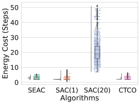
Figure 6: In the difficult version of the maze game, we looked at the energy used in 1,000 tries. SEAC used fewer steps than SAC (20 Hz). Even though SEAC and SAC at 1 Hz were similar in steps, SEAC was faster. So, when we compare it to SAC with a fixed control rate, SEAC uses less energy. While SEAC might use more steps (energy) compared to CTCO, the total number of steps is similar. This arises because CTCO does not prioritize the time it takes to complete a task. We didn’t include SAC (100 Hz) because its policy model didn’t converge.

Figure 6 shows the energy costs (measured in the number of time steps) for 1,000 separate trials in the difficult version of the maze game. While SEAC uses a similar number of steps as CTCO and SAC (1 Hz), Figure 7 clearly demonstrates that SAC takes considerably more energy than SEAC. CTCO demonstrates similar, even better energy consumption performance than SEAC, primarily because it does not factor in the time required to complete a task. Although the discount factor $\gamma$ ensures a minimum number of steps, it doesn’t necessarily equate to the least time for task completion. This distinction is important in evaluating the overall efficiency of these models.

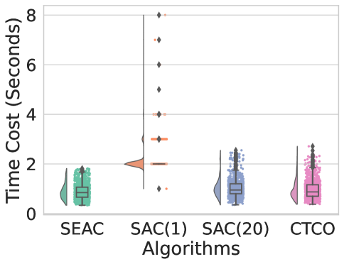
Figure 7: In the difficult version of the maze game, we checked how much time is used in 1,000 tries. SEAC finished tasks faster than both SAC (1 Hz) and SAC (20 Hz). This means SEAC is quicker compared to SAC with a fixed control rate. Our statistical analysis reveals that SEAC has a lower average task completion time and less variance than CTCO. This indicates that SEAC outperforms CTCO in terms of time efficiency. We left out SAC at 100 Hz because its policy model didn’t converge.

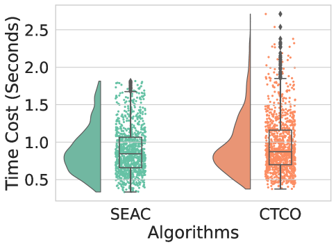
Figure 8: We specifically chose SEAC and CTCO from Figure 7 to highlight their differences, which aren’t clear due to the impact of SAC (1 Hz) on the Y-axis. While CTCO also performs well in terms of time, it exhibits less average value, more significant variance, and outliers than SEAC. If the time range for each step is broader, or more steps are required to complete the task, these results become more pronounced.

Figure 7 presents the time taken per task for these 1,000 trials. SEAC outperforms both SAC (1 Hz) and SAC (20 Hz) in terms of speed and stability. SEAC exhibits a lower average task time and reduced variance compared to CTCO. To evaluate these differences, we conducted a series of one-tailed T-tests [30] and F-tests [31] on a dataset comprising 1,000 sets. We hypothesized that SEAC would demonstrate a shorter average time and a more minor variance than CTCO. The outcomes of these statistical tests are presented in Table IV, providing quantitative support for our assessment.

TABLE IV: T-test and F-test results of time performance of SEAC and CTCO

State and action information of Trackmani
	T (F) value	p value
T-test	$-4.769$	$9.909e^{-7}$
F-test	$1.441$	$4.300e^{-9}$

The t-test resulted in a t-value of -4.769, indicating that SEAC’s average time is shorter than that of CTCO. The very low p-value, much lower than standard thresholds of 0.05 or 0.01, points to a statistically significant difference between the average times of the two groups. The negative t-value, in conjunction with the one-tailed nature of the test, strongly supports the conclusion that SEAC’s average time is significantly lower than CTCO’s.

Furthermore, the F-test produced an F-value of 1.441 with an exceedingly low p-value. An F-value greater than 1 suggests that CTCO’s time variance is higher than SEAC’s. The small p-value confirms the statistical significance of this variance difference. While the F-test is inherently two-tailed, the nature of the F-value calculation (more considerable variance divided by more minor variance) indicates that the variability in SEAC’s times is notably lower than in CTCO’s.

In conclusion, the results of these statistical tests solidly affirm that SEAC not only has a lower average time compared to CTCO but also demonstrates significantly less variability in its timing. This points to SEAC being more efficient and consistent than CTCO regarding time performance. We display them individually in Figure 8 to make it easier for readers to see their differences.

In summary, SEAC reduces energy and time usage and achieves a high reward compared with SAC. SEAC and CTCO have similar training speed and energy consumption, but SEAC is stronger than CTCO in terms of time performance. We ensured a consistent starting point for all algorithms in this analysis using the same seed, guaranteeing fairness and consistency in our results.

V-B Results of the Trackmania 2023

Our SEAC strategy model achieved a lap time of 45.808 seconds in the car race simulation despite encountering two collisions. This time was slightly better than the record previously set by the TMRL team [2]. We have recorded the entire race on video to provide a comprehensive view of the model’s performance, including the collision instances.

We also show the changes in the control rate of the car at lower right corner of video. We also provide additional raincloud graphs (Figure 9 and 10)) of energy and time consumption for 30 races compared to SAC (20 Hz). Appendix -B provides all hyperparameter settings and implementation details.

By analyzing the video, we draw several conclusions about the SEAC model’s performance:

1. In dynamic areas such as turns, where the visual input changes rapidly, the SEAC model tends to use a higher control rate. This approach helps maintain speed and manage disturbances like random environmental delays. Conversely, in less control-demanding sections like straight paths, it lowers the control rate to reduce computational energy use. These results align with our initial expectations.

2. At areas where straight paths and curves intersect, the model adjusts to a control rate of around 16-18 Hz. This is to handle unpredictable changes, as the input relies solely on images and the agent lacks global location awareness.

3. Both collisions occurred shortly after periods of low-frequency control, suggesting that random delays and inertia in the environment might have contributed to these incidents. Interestingly, a similar pattern of 1-2 collisions was unavoidable even when using the SAC model strategy at a constant 20 Hz control rate.

However, as noted in Section III-B, while simulating collisions, the Trackmania 2023 game’s physics engine does not include an item damage mechanism or provide an API for collision detection. Consequently, we can’t identify collisions through images or APIs. This limitation means that modifying the reward function, such as increasing penalties for collisions as in our maze game, is currently not feasible for preventing collisions in this context.

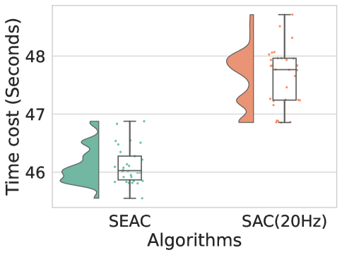
Figure 9: In our tests on the Trackmania 2023 map, we measured the time taken for 30 attempts. Generally, SEAC completed the games faster than SAC (20 Hz) in most tasks. This indicates that SEAC is more efficient in terms of speed compared to SAC.

Figure 9 leads us to a conclusion similar to what we got in the Maze game. Generally, SEAC takes less time than SAC (20 Hz). In this game, which requires real-time control strategies, SEAC performed well, demonstrating its capability and potential to tackle complex challenges. However, since the training is real-time, we couldn’t fully showcase the benefits of SEAC’s faster training speed, which is regrettable. We hope that more gym or game environments, particularly those involving continuous control strategies like in robot simulations like Mujoco [32], will allow for varying control rates.

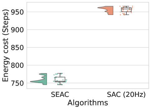
Figure 10: In our tests on the Trackmania 2023 map, we measured the energy cost (number of steps) taken for 30 attempts. SEAC completed the games using fewer steps than SAC (20 Hz) in all tasks. This indicates that SEAC is more efficient than SAC regarding energy cost.

Figure 10 illustrates that SEAC’s average computing energy consumption for completing tasks is substantially lower than SAC (20 Hz). The average energy consumption is reduced by about 20% with SEAC, and it also completes tasks in less time compared to the SAC baseline.

This approach of using flexible time steps in reinforcement learning, as opposed to fixed time steps, greatly enhances data efficiency. Our experiments in various practical applications have shown that this method is a promising approach in the field of continuous control reinforcement learning.

VI Conclusions

In this paper, we apply a variable-control-rate-based reward policy that we proposed recently to maze games and the Trackmania 2023 racing game. It allows the agent to change the control frequency adaptively by simultaneously outputting action values and durations during the reinforcement learning process, thereby reducing energy consumption and time and improving data efficiency. Reducing the amount of computation makes a lot of sense when using robots with limited computing power. This reduction allows us to use the saved computing power for other purposes, like environmental awareness, communication, or mapping. Additionally, the decreased computing demand means we can run more demanding models on devices with limited computing capabilities, like Raspberry Pi.

We compared our SEAC with CTCO and fixed-control-rate SAC. SEAC and CTCO are comparable in training speed and energy usage. However, SEAC outperforms CTCO regarding time performance, indicating its greater efficiency in this aspect. SEAC is superior to the SAC algorithm regarding training speed and final performance.

In our previous work, we didn’t discuss how the three parameters ($\alpha_{task}$, $\alpha_{\epsilon}$ and $\alpha_{tau}$) of our reward policy affect the convergence of the reinforcement learning process. While these parameters speed up training compared to fixed-control-rate reinforcement learning, increasing them complicates the adjustment of the learning parameters. Based on our research, we offer some suggestions:

1. $\alpha_{\epsilon}$ and $\alpha_{tau}$ determine the size of the rewards related to energy and time loss, respectively. We suggest balancing the rewards for energy and time loss at each step. This balance helps the learning process to choose between reducing time and minimizing steps effectively.

2. If the reinforcement learning with elastic time steps struggles to converge, consider increasing $\alpha_{task}$. A high proportion of energy and time loss rewards can overshadow the task rewards, affecting the learning incentives.

Our findings enhance the conception that the control rate can significantly impact continuous control method reinforcement learning. And we figure out that its impact is not only on the training speed but also on whether the final results converge. The reinforcement learning with elastic time steps method we proposed based on the reactive control principle can solve the problem of optimal control rate and achieve tasks quickly and energy-savingly. Its performance surpasses that of the fixed control rate SAC. Moreover, it outperforms CTCO, the only other variable control frequency algorithm in the community besides ours. We invite readers to refer to Section V-B and Appendix -A for more information.

Our method enhances the data efficiency and energy-saving aspects of reinforcement learning, proven in the real-time control strategy game Trackmania 2023. For implementation details, please refer to Section V-B and Appendix -B.

Our upcoming objective is to implement our method in real-world robotics, including smart cars, robotic arms, and similar technologies. We have established the potential of our SEAC algorithm both in theory and through practical applications. We are confident that our algorithm will demonstrate strong performance in robotic applications, which will be the primary focus of our forthcoming work.

-A Hyperparameters Setting of SEAC on Maze Games

Hyperparameter sheet
Name	Value	Annotation
Total steps	$3e6$
$\gamma$	$0.99$	Discount factor
Net shape	$(256,256)$
batch_size	$256$
a_lr	$3e5$	Learning rate of Actor Network
c_lr	$3e5$	Learning rate of Critic Network
$\epsilon$	$1.0$	Energy cost per step
$\alpha_{task}$	$1.0$	Gain coefficient of task reward
$\alpha_{\epsilon}$	$0.1$	Gain coefficient of energy reward
$\alpha_{\tau}$	$0.1$	Gain coefficient of time reward
max_steps	$500$	Maximum steps for one episode
$\alpha$	$0.12$
$\eta$	$-3$	Refer to SAC [3]
$T_{i}$	$1.0,20.0,100.0$	Time duration of rest compared RL algorithms, in HZ
min_frequency	$1.0$	Minimum control frequency, in HZ
max_frequency	$100.0$	Maximum control frequency, in HZ
Optimizer	Adam	Refer to Adam [33]
environment steps	$1$
Replaybuffer size	$1e5$
Number of samples before training start	$5\cdot max\_steps$
Number of critics	$2$

-B Hyperparameters Setting of SEAC on Trackmania 2023

Hyperparameter sheet
Name	Value	Annotation
Total steps	$5e6$
$\gamma$	$0.995$	Discount factor
Net shape	$(256,256)$
batch_size	$256$
a_lr	$1e5$	Learning rate of Actor Network
c_lr	$2e5$	Learning rate of Critic Network
$\epsilon$	$1.0$	Energy cost per step
$\alpha_{task}$	$3.0$	Gain coefficient of task reward
$\alpha_{\epsilon}$	$0.01$	Gain coefficient of energy reward
$\alpha_{\tau}$	$0.1$	Gain coefficient of time reward
max_steps	$1000$	Maximum steps for one episode
$\alpha$	$0.12$
$\eta$	$-4$	Refer to SAC [3]
min_frequency	$5.0$	Minimum control frequency, in HZ
max_frequency	$30.0$	Maximum control frequency, in HZ
Optimizer	Adam	Refer to Adam [33]
environment steps	$1$
Replaybuffer size	$1e5$
Number of samples before training start	$5\cdot max\_steps$
Number of critics	$2$

Dong Wang (Member, IEEE) received his bachelor’s degree in electronic engineering from the School of Aviation, Northwestern Polytechnical University (NWPU), Xi’an, China, in 2017. He is pursuing his Ph.D. in the Department of Software Engineering at Polytechnique Montreal, Montreal, Canada. His research interests include reinforcement learning, computer vision, and robotics.

Giovanni Beltrame Giovanni Beltrame (Senior Member, IEEE) received the Ph.D. degree in computer engineering from Po- litecnico di Milano, Milan, Italy, in 2006. He worked as a Microelectronics Engineer with the European Space Agency, Paris, France, on a number of projects, spanning from radiation tolerant systems to computer-aided design. Since 2010, he has been the Professor with the Computer and Software Engineer- ing Department, Polytechnique Montreal, Montreal, QC, Canada, where he directs the MIST Lab. He has authored or coauthored more than 150 papers in international journals and conferences. His research interests include modeling and design of embedded systems, artificial intelligence, and robotics.

References

- [1] D. Silver, A. Huang, C. J. Maddison, A. Guez, L. Sifre, G. Van Den Driessche, J. Schrittwieser, I. Antonoglou, V. Panneershelvam, M. Lanctot et al., “Mastering the game of go with deep neural networks and tree search,” nature, vol. 529, no. 7587, pp. 484–489, 2016.
- [2] tmrl, “tmrl main page,” https://github.com/trackmania-rl/tmrl, 2023.
- [3] T. Haarnoja, A. Zhou, K. Hartikainen, G. Tucker, S. Ha, J. Tan, V. Kumar, H. Zhu, A. Gupta, P. Abbeel et al., “Soft actor-critic algorithms and applications,” arXiv preprint arXiv:1812.05905, 2018.
- [4] P. R. Wurman, S. Barrett, K. Kawamoto, J. MacGlashan, K. Subramanian, T. J. Walsh, R. Capobianco, A. Devlic, F. Eckert, F. Fuchs et al., “Outracing champion gran turismo drivers with deep reinforcement learning,” Nature, vol. 602, no. 7896, pp. 223–228, 2022.
- [5] J. Li, J. Ding, T. Chai, F. L. Lewis, and S. Jagannathan, “Adaptive interleaved reinforcement learning: Robust stability of affine nonlinear systems with unknown uncertainty,” IEEE Transactions on Neural Networks and Learning Systems, vol. 33, no. 1, pp. 270–280, 2020.
- [6] Anonymous, “Reinforcement learning with elastic time steps,” 2024. [Online]. Available: https://openreview.net/forum?id=riQmzq5FaQ
- [7] D. Wang and G. Beltrame, “Deployable reinforcement learning with variable control rate,” arXiv preprint arXiv:2401.09286, 2024.
- [8] S. Amin, M. Gomrokchi, H. Aboutalebi, H. Satija, and D. Precup, “Locally persistent exploration in continuous control tasks with sparse rewards,” arXiv preprint arXiv:2012.13658, 2020.
- [9] S. Park, J. Kim, and G. Kim, “Time discretization-invariant safe action repetition for policy gradient methods,” Advances in Neural Information Processing Systems, vol. 34, pp. 267–279, 2021.
- [10] Y. Bouteiller, S. Ramstedt, G. Beltrame, C. Pal, and J. Binas, “Reinforcement learning with random delays,” in International conference on learning representations, 2021.
- [11] T. Haarnoja, A. Zhou, P. Abbeel, and S. Levine, “Soft actor-critic: Off-policy maximum entropy deep reinforcement learning with a stochastic actor,” in International conference on machine learning. PMLR, 2018, pp. 1861–1870.
- [12] A. Karimi, J. Jin, J. Luo, A. R. Mahmood, M. Jagersand, and S. Tosatto, “Dynamic decision frequency with continuous options,” in 2023 IEEE/RSJ International Conference on Intelligent Robots and Systems (IROS). IEEE, 2023, pp. 7545–7552.
- [13] S. Sharma, A. Srinivas, and B. Ravindran, “Learning to repeat: Fine grained action repetition for deep reinforcement learning,” arXiv preprint arXiv:1702.06054, 2017.
- [14] A. M. Metelli, F. Mazzolini, L. Bisi, L. Sabbioni, and M. Restelli, “Control frequency adaptation via action persistence in batch reinforcement learning,” in International Conference on Machine Learning. PMLR, 2020, pp. 6862–6873.
- [15] J. Lee, B.-J. Lee, and K.-E. Kim, “Reinforcement learning for control with multiple frequencies,” Advances in Neural Information Processing Systems, vol. 33, pp. 3254–3264, 2020.
- [16] T. G. Dietterich, “Hierarchical reinforcement learning with the maxq value function decomposition,” Journal of artificial intelligence research, vol. 13, pp. 227–303, 2000.
- [17] U. T. 2023, “Trackmania main page,” https://www.ubisoft.com/en-us/game/trackmania/trackmania, 2023.
- [18] Y. Chen, H. Wu, Y. Liang, and G. Lai, “Varlenmarl: A framework of variable-length time-step multi-agent reinforcement learning for cooperative charging in sensor networks,” in 2021 18th Annual IEEE International Conference on Sensing, Communication, and Networking (SECON). IEEE, 2021, pp. 1–9.
- [19] S. Nasiriany, H. Liu, and Y. Zhu, “Augmenting reinforcement learning with behavior primitives for diverse manipulation tasks,” in 2022 International Conference on Robotics and Automation (ICRA). IEEE, 2022, pp. 7477–7484.
- [20] F. Pardo, A. Tavakoli, V. Levdik, and P. Kormushev, “Time limits in reinforcement learning,” in International Conference on Machine Learning. PMLR, 2018, pp. 4045–4054.
- [21] Z. Zhang, D. Zhang, and R. C. Qiu, “Deep reinforcement learning for power system applications: An overview,” CSEE Journal of Power and Energy Systems, vol. 6, no. 1, pp. 213–225, 2019.
- [22] Z. Yang, K. Merrick, L. Jin, and H. A. Abbass, “Hierarchical deep reinforcement learning for continuous action control,” IEEE transactions on neural networks and learning systems, vol. 29, no. 11, pp. 5174–5184, 2018.
- [23] Raspberrypi, “Raspberrypi main page,” https://www.raspberrypi.com/, 2023.
- [24] E. Bregu, N. Casamassima, D. Cantoni, L. Mottola, and K. Whitehouse, “Reactive control of autonomous drones,” in Proceedings of the 14th Annual International Conference on Mobile Systems, Applications, and Services, 2016, pp. 207–219.
- [25] gymnasium, “Gymnasium main page,” https://gymnasium.farama.org/content/basic_usage/, 2023.
- [26] Openplanet, “Openplanet main page,” https://openplanet.dev/, 2023.
- [27] I. J. Balaban, “An optimal algorithm for finding segments intersections,” in Proceedings of the eleventh annual symposium on Computational geometry, 1995, pp. 211–219.
- [28] Rtgym, “Rtgym main page,” https://github.com/yannbouteiller/rtgym/releases, 2023.
- [29] K. O’Shea and R. Nash, “An introduction to convolutional neural networks,” arXiv preprint arXiv:1511.08458, 2015.
- [30] T. K. Kim, “T test as a parametric statistic,” Korean journal of anesthesiology, vol. 68, no. 6, pp. 540–546, 2015.
- [31] L. M. Lix, J. C. Keselman, and H. J. Keselman, “Consequences of assumption violations revisited: A quantitative review of alternatives to the one-way analysis of variance f test,” Review of educational research, vol. 66, no. 4, pp. 579–619, 1996.
- [32] E. Todorov, T. Erez, and Y. Tassa, “Mujoco: A physics engine for model-based control,” in 2012 IEEE/RSJ international conference on intelligent robots and systems. IEEE, 2012, pp. 5026–5033.
- [33] D. P. Kingma and J. Ba, “Adam: A method for stochastic optimization,” arXiv preprint arXiv:1412.6980, 2014.