Signals of Detailed Balance Violation in Nonequilibrium Stationary States: Subtle, Manifest, and Extraordinary

Abstract

The evolution of physical systems are often modeled by simple Markovian processes. When settled into stationary states, the probability distributions of such systems are time independent, by definition. However, they do not necessarily fall within the framework of equilibrium statistical mechanics. Instead, they may be non-equilibrium steady states (NESS). One distinguished feature of NESS is the presence of time reversal asymmetry (TRA) and persistent probability current loops. These loops lead naturally to the notion of probability angular momenta, which play a role on the same footing as the noise covariance in stochastic processes. Illustrating with simulations of simple models and physical data, we present ways to detect these signals of TRA, from the subtle to the prominent.

I Introduction

To formulate a theory of equilibrium statistical mechanics, the principle of detailed balance (DB) played a foundational role for both Boltzmann and Maxwell. Based on the laws of classical physics, it embodies the notion of time reversal invariance. The key theme is that, once it “settled down into a stationary state,” the evolution of an isolated system is (statistically) the same whether time is reversed or not. A favorite way to put this notion in layman’s terms is the following: If you are shown a movie of a system in thermal equilibrium, you cannot tell if the movie is run forwards or backwards. A more sophisticated way to describe this state is that its entropy has reached its maximum and cannot increase further.

If a system is not in isolation, but in contact with multiple reservoirs which are not in equilibrium, then the dynamics of these reservoirs may lead to a flow of energy (or matter, or information, or …) through our system. Good examples include all forms of life on Earth as well as our entire ecosystem. All life forms take in nutrients and discard waste, while our ecosystem is sustained by a balance between incoming solar radiation and outgoing IR rays. When the time-scales of these reservoirs are long enough (and spatial scales large enough), then it is conceivable for our (comparatively small) system to settle into a “quasi-stationary state” (i.e., stationary over much shorter time-scales). Clearly, it is prohibitively challenging to describe such a system as well as its “environment” – the large, slowly varying reservoirs. An approximate description is to focus on our system alone and model its evolution with a stochastic dynamics that is not time-reversal invariant, i.e., with DB violating rules. When such a system settles down, it will be in a non-equilibrium steady state (NESS), while a movie of it run forwards should be distinguishable from one run backwards. What are the signals of such time-reversal asymmetry (TRA)? We will present both generally applicable and comprehensible results, as well as specific examples which range from the readily solvable to the most challenging.

To discuss stochastic processes in general is beyond the scope of this article. Instead, we limit ourselves here to noisy systems that can be modeled by Markovian dynamics. Starting with the conceptually easy Langevin approach for a single particle, as well as the equivalent Fokker-Planck description, we will move on to arbitrary systems with finite and discrete configurations ($\mathcal{C}_{i};~{}i=1,...,N$) evolving stochastically in discrete time steps ($\tau$) with time independent rates $R\left(i|j\right)$. There, the focus will be on the distribution $P\left(i,\tau\right)$ – the probability to find our system in $\mathcal{C}_{i}$ at time $\tau$ – given an initial condition $P\left(k,0\right)$. By limiting ourselves this way, the full evolution can be specified by a Master equation for $P$, based on a given set $R$’s. The next Section will be devoted to these different set ups. As a linear equation for a finite number of variables, the Master equation is, in principle, solvable. The remainder of this article consists of expanding on the notion of DB, the existence of non-trivial probability currents, and TRA in NESS. Generalities will be presented in in Section III, with the main focus on probability angular momenta. Its relationship with ordinary angular momenta and, remarkably, the covariance of the noise, will be highlighted in Subsection III.1.1. Though most of this article will focus on probability angular momenta, a short digression will be introduced (Subsection III.2) to discuss “one dimensional” systems, which do not ordinarily support angular momenta. In Section IV, we present a number of illustrations, from simple simulation to physical data. They show a range of systems which display signals of DB violation and TRA, from the “subtle” to the “manifest.” Beyond, we emphasize that DB violation can also lead to NESS with astonishingly unexpected phenomena, such as all living organisms. This level of “extraordinary” behavior will be illustrated in a simple example – one recently studiedDZ18 ; LDZ21 in the context of driven diffusive systems. Several appendices contain much of the mathematical details of our discussions. We end with a brief summary and outlook.

II Equations for stochastic processes and stationary distributions $P^{\ast}$

There are several equivalent ways to describe a stochastic process. Conceptually, arguably the simplest is the Langevin approachLangevin , where noise is incorporated into equations of evolution for the degrees of freedom of interest. In the example of a single particle moving in ordinary space-time $\left(\vec{x},t\right)$, the Langevin equation reads $m\partial_{t}^{2}\vec{x}=\vec{F}+\vec{\eta}$. Here $\vec{\eta}$ is a random force, often chosen as Gaussian distributed, with zero mean and constant variance, uncorrelated from one time to another. The histories, $\vec{x}\left(t\right)$’s, resulting from different realizations of $\vec{\eta}$ form “spaghetti plots” (as often seen in hurricane forecasts), which provide a rough sense of $P(\vec{x},t)$, the probability of finding it at $\vec{x}$ at time $t$. An alternative is the deterministic Fokker-Planck equationFokker for $P$, while standard methods link one description to the other. The simplest version of the former (representing the over-damped, $m\rightarrow 0$ limit of $\vec{F}=m\vec{a}$) is

$$\partial_{t}\vec{x}=\vec{\mu}+\vec{\eta};~{}~{}\left\langle\vec{\eta}\vec{\eta}^{T}\right\rangle\propto 2\mathbb{D}$$ (1)

It is equivalent to drift with diffusion in the latter:

$$\partial_{t}P=-\vec{\nabla}\cdot\left[\vec{\mu}P-\mathbb{D}\vec{\nabla}P\right]$$ (2)

In these approaches, the particle is allowed to take only infinitesimal steps in both $\vec{x}$ and $t$. Obviously, these equations can be generalized to many variables (to be denoted by $\xi_{\alpha}$ below) evolving in continuous $t$.

The Master equation is a generalization, in that all type of stochastic processes can be modeled, beyond the bounds of infinitesimal steps in continuous space-time. For example, we may consider the dollar value of a stock from one trading session to the next, the number of individuals infected with COVID-19 from week to week, or the state of $L^{d}$ spins of an Ising model in a $d$-dimensional cubic lattice, flipping in a Monte-Carlo simulation.

To keep the presentation here simple and to relate directly to simulation studies, let us consider systems with discrete configurations $\mathcal{C}_{i}$ evolving in discrete time steps (of unit $\varepsilon$). For short, we will use $i$ and $\tau=0,\varepsilon,2\varepsilon,...$ (in lieu of continuous $\vec{x},t$). The stochastic evolution of the distribution $P\left(i,\tau\right)$ is completely specified by an initial $P\left(k,0\right)$ and the set of “rates” $R\left(i|j\right)\geq 0$ for $i\neq j$. In general, these $R$’s are time dependent. But, to keep our problem manageable, we will restrict ourselves to $t$-independent ones here. The Master equation specifies the change in $P$ from one $\tau$ to the next:

$$\Delta_{\tau}P\left(i,\tau\right) \equiv P\left(i,\tau+\varepsilon\right)-P\left(i,\tau\right)$$ (3)

$$=\sum_{j\neq i}\left[R\left(i|j\right)P\left(j,\tau\right)-R\left(j|i\right)P\left(i,\tau\right)\right]$$ (4)

It is clear that the two terms in Eqn.(4) represent the “flow of probability into $\mathcal{C}_{i}$” and “out from $\mathcal{C}_{i}$,” respectively. Obviously, $R\left(i|j\right)$ can be regarded as the conditional probability for finding $i$ given $j$, while $R\left(i|j\right)P\left(j,\tau\right)$ is just the joint probability $\mathcal{P}\left(i,\tau+\varepsilon\cap j,\tau\right)$ for finding the system in configuration $\mathcal{C}_{j}$ at $\tau$ and in $\mathcal{C}_{i}$ at $\tau+\varepsilon$. Note that, in this formulation, there is no mention of a metric in $\mathcal{C}$ space, and there is no restriction on how “close” $\mathcal{C}_{i}$ and $\mathcal{C}_{j}$ must be. Unlike the Fokker-Planck equation, the Master equation can describe a system that may “jump” from any $\mathcal{C}$ to any other one in the system. By introducing some notion of distance in $\mathcal{C}$ space (e.g., ordinary space $\vec{x}$) and allowing only “infinitesimally close moves” in infinitesimal time steps, we can recover a Fokker-Planck equation from the Master equation by taking appropriate continuum limits.

Next, we turn to the problem of “solving” these equations. Being a stochastic differential equation, the solution to the Langevin equation, $\vec{x}\left(t\right)$, will be different for each realization of the noise $\vec{\eta}\left(t\right)$. In principle, statistical analysis, using a given distribution for the noise, needs to be performed to obtain averages and correlations like $\left\langle\vec{x}\left(t\right)\right\rangle$ and $\left\langle\vec{x}\left(t\right)\vec{x}\left(t^{\prime}\right)\right\rangle$. The Fokker-Planck equation for $P$ is deterministic and linear (like the Schrödinger equation for $\Psi(\vec{x},t)$) and finding $P(\vec{x},t)$ in general is as difficult as solving for $\Psi(\vec{x},t)$ in quantum mechanics. Formally, the approach in non-relativistic quantum mechanics can be followed, by writing the right hand side of Eqn.(2) as an operator – the Liouvillian $\mathfrak{L}$ – on $P$. Then the solution $P\left(t\right)$, given some initial distribution, $P\left(0\right)$, is just $\exp\left[\mathfrak{L}t\right]P\left(0\right)$. The same strategy can be applied to the Master equation (3). Regarding $P\left(i,\tau\right)$ as a ket $\left|P_{\tau}\right\rangle$, we can write the equation in a compact form:

$$\Delta_{\tau}\left|P\right\rangle=\mathfrak{L}\left|P\right\rangle\implies\left|P_{\tau+\varepsilon}\right\rangle=\left(\mathfrak{I}+\mathfrak{L}\right)\left|P_{\tau}\right\rangle$$

where $\mathfrak{I}$ is the identity matrix. Here, the off-diagonal elements of $\mathfrak{L}$ are the $R$’s, while the $i^{th}$ diagonal element is the sum $[-\sum_{j\neq i}R\left(j|i\right)]$. Given some initial distribution $\left|P_{ini}\right\rangle$, the full solution is just

$$\left|P_{\tau}\right\rangle=\left(\mathfrak{I}+\mathfrak{L}\right)^{\tau}\left|P_{ini}\right\rangle$$

Of course, this expression is somewhat formal and a practical solution will require finding all the eigenvalues and eigenvectors (both right- and left-eigenvectors, or kets and bras) of $\mathfrak{L}$ :

$$\mathfrak{L}\left|u_{A}\right\rangle=\lambda_{A}\left|u_{A}\right\rangle;~{}~{}\left\langle w_{A}\right|\mathfrak{L}=\lambda_{A}\left\langle w_{A}\right|$$

so that $\left|P_{\tau}\right\rangle=\sum_{A}\left|u_{A}\right\rangle\left(1+\lambda_{A}\right)^{\tau}\left\langle w_{A}\right|\left.P_{ini}\right\rangle$.

In general, such a task would be prohibitively difficult. However, as $\mathfrak{L}$ describes a stochastic process for probabilities, it has special properties: First, since probability is conserved, $\Delta_{\tau}\sum_{i}\left|P\right\rangle\equiv 0$, so that $\left\langle w_{0}\right|=\left(1,1,1,...,1\right)$ must be a bra with $\lambda_{0}\equiv 0$. Associated with this is a ket $\left|u_{0}\right\rangle$, which is readily recognized as a steady state, as it does not change from one $\tau$ to the next. Denoting $\left|u_{0}\right\rangle$ by $\left|P^{\ast}\right\rangle$, it is naturally normalized by $1=$ $\left\langle w_{0}\right|\left.P^{\ast}\right\rangle$. The issue of other zero eigenvalues and uniqueness of the pair, $\left\langle w_{0}\right|$ and $\left|u_{0}\right\rangle$, is not trivial and will not be addressed in this short article. We will restrict ourselves to systems in which $\left|P^{\ast}\right\rangle$ is unique. Next, thanks to Perron-Frobenius PF-wiki , all $\lambda$’s besides $\lambda_{0}$ have real parts in $\left[-1,0\right)$, so that $\left|P\right\rangle$ will reach $\left|P^{\ast}\right\rangle$ at large times. Much of the rest of this article will focus on this steady state $\left|P^{\ast}\right\rangle$ and its properties.

For $\Delta_{\tau}\left|P^{\ast}\right\rangle=0$, it is sufficient (but not necessary) if each term within $\left[...\right]$ of Eqn.(4) vanishes:

$$R\left(i|j\right)P^{\ast}\left(j\right)=R\left(j|i\right)P^{\ast}\left(i\right)$$ (5)

a condition often referred to as detailed balance (DB). Note that, in terms of $\mathcal{P}^{\ast}$, the joint probability in the steady state, this condition takes the form

$$\mathcal{P}^{\ast}\left(i,\tau+\varepsilon\cap j,\tau\right)=\mathcal{P}^{\ast}\left(j,\tau+\varepsilon\cap i,\tau\right)$$ (6)

The DB condition allows us to exploit computer simulations and generate a set of configurations that approximate the relative probabilities of a system in thermal equilibrium (e.g., $P^{\ast}\left(i\right)\propto\exp\left\{-\mathcal{H}\left(\mathcal{C}_{i}\right)\right\}$, where $\mathcal{H}$ is an energy functional). In particular, it suffices to employ any set of $R$’s that obeys (5). However, if we are only given a set of $R$’s which specifies a Markovian process, then we typically do not have $P^{\ast}\left(i\right)$ a priori, and checking if the $R$’s satisfy DB or not requires more effort. Not being the focus here, we will just list some references for the interested readerW11 ; Komo36 ; ZS07 .

The crux of the issue here is that individual terms on the right of Eqn.(4) need not vanish, only their sum (at each $i$) must do so. Indeed, since probability is conserved, each term in the sum is recognized as the net probability currentZS07 , from $\mathcal{C}_{j}$ to $\mathcal{C}_{i}$: $K\left(i|j,\tau\right)\equiv R\left(i|j\right)P\left(j,\tau\right)-R\left(j|i\right)P\left(i,\tau\right)$. When the system settles in the steady state, there is no constraint that the time-independent currents

$$K^{\ast}\left(i|j\right) \equiv R\left(i|j\right)P^{\ast}\left(j\right)-R\left(j|i\right)P^{\ast}\left(i\right)$$ (7)

$$=\mathcal{P}^{\ast}\left(i,\varepsilon\cap j,0\right)-\mathcal{P}^{\ast}\left(j,\varepsilon\cap i,0\right)$$ (8)

must vanish. Instead, since $\Delta_{\tau}\left|P^{\ast}\right\rangle=0$, these persistent $K^{\ast}$’s sum to zero at each $i$ and so, they must form closed loops. Such states are analogous to those in magnetostatics. In this electromagnetic analog, we distinguish time-independent states by referring those with $K^{\ast}\equiv 0$ (à la electrostatics) as “equilibrium steady states” and those with $K^{\ast}\neq 0$ as “non-equilibrium steady states” – NESS. While the former can be achieved by being totally isolated (the micro-canonical ensemble) or being in equilibrium with one or more, much larger, reservoirs (e.g., energy reservoir and the canonical ensemble or particle reservoir and the grand ensemble), the latter are open systems, typically coupled to multiple reservoirs in such a way as to allow a steady flux of energy (or matter, or …) through them. Such throughput prevents our system from ever reaching thermal equilibrium and sets up non-trivial, persistent $K^{\ast}$’s in NESSs.

In the Fokker-Planck formulation, these considerations take a slightly different form. Conserving probability, Eqn.(2) is just a continuity equation, e.g., $\partial_{t}\rho=-\vec{\nabla}\cdot\vec{J}$. Thus, the probability currents here are “vector fields”: $\vec{J}_{FP}=\vec{\mu}P-\mathbb{D}\vec{\nabla}P$, with zero divergence in a NESS: $\vec{\nabla}\cdot\vec{J}_{FP}^{\ast}=0$. Analogous to the usual relation $\vec{J}=\rho\vec{v}$, we may regard $\vec{J}_{FP}/P=\vec{\mu}-D\vec{\nabla}\ln P$ as the “probability velocity field”. However, $\vec{J}_{FP}$ is not the same as $K$, as the former requires the notion of metric on the space of configurations (e.g., ordinary $\vec{x}$ or the more general $\xi_{\alpha}$) and transitions to be infinitesimally “close” (for $\vec{v}$ to be well defined). If we discretize $\vec{x}$ and write an approximate version of Eqn.(2) in matrix form, the presence of $\nabla$ and $\nabla^{2}$ implies that its $R\left(i|j\right)$’s would be zero for $i,j$ being further than nearest neighbor pairs, say. In this sense, we regard the Master equation as more general, with no restrictions on $R$. Though $\vec{J}_{FP}$ and $K$ are different, the DB condition still takes the form $\vec{J}_{FP}^{\ast}=0$, and is a property of $\vec{\mu}$ and $\mathbb{D}$. Clearly, $\vec{J}_{FP}^{\ast}\neq 0$ in a NESS but must be “a curl,” i.e., divergence of an anti-symmetric tensor field. Thus, we have the concept of current loops here, much like in magnetostatics.

To summarize, systems evolving with DB respecting $R$’s will settled into equilibrium stationary states with $K^{\ast}\equiv 0$ and a readily obtainable $P^{\ast}$, while systems subjected to DB violating $R$’s will settle into NE steady states. Generally, given DB violating $R$’s, the distribution $P^{\ast}$ is unknown (though a formal solution exists Hill66 ; ZS07 ), while some non-trivial, persistent current loops will be present. Exploring the consequences of these $K^{\ast}$’s were initiated sometime agoZS07 . The remainder of this article will be devoted to more recent efforts: detecting various signals of DB violation in NESS, ranging from quite subtle ones and clearly self-evident ones to those displaying extraordinary, unexpected phenomena.

III Detailed balance violation and time reversal asymmetry in NESS

In a stochastic process, $P\left(i,\mathcal{\tau}\right)$ may seem abstract and unmanageable. Instead, we may focus on expectation values of observables. Denoting the observables as $\mathcal{O}\left(i\right)$ – functionals of the configurations $\mathcal{C}_{i}$, the expectations at time $\tau$ are

$$\left\langle\mathcal{O}\right\rangle_{\mathcal{\tau}}\equiv\sum_{i}\mathcal{O}\left(i\right)P\left(i,\mathcal{\tau}\right)$$

By definition, a system in steady state is invariant under time translation, i.e., $\left\langle\mathcal{O}\right\rangle_{\mathcal{\tau}}=\left\langle\mathcal{O}\right\rangle_{\mathcal{\tau}+\upsilon}$ for any $\upsilon$ and are denoted by

$$\left\langle\mathcal{O}\right\rangle^{\ast}\equiv\sum_{i}\mathcal{O}P^{\ast}\left(i\right)$$

Thanks to this property, simulation studies of steady states often replace ensemble averages, $\left\langle\cdot\right\rangle^{\ast}$, by time averages, $\overline{{\Large\cdot}}$, over a single long run (or very few runs). In examples of simulation results we present below, $\left\langle\cdot\right\rangle^{\ast}$ are obtained from such time averages.

It is clear that, to detect time reversal asymmetry in steady states, we must start with expectations of observables at different times, e.g.,

$$\left\langle\mathcal{O}^{\prime}\mathcal{O}\right\rangle_{\mathcal{\tau}^{\prime},\mathcal{\tau}}\equiv\sum_{i,i^{\prime}}\mathcal{O}^{\prime}\!\left(i^{\prime}\right)\mathcal{O}\left(i\right)\mathcal{P}\left(i^{\prime},\mathcal{\tau}^{\prime}\cap i,\mathcal{\tau}\right)$$ (9)

Due to translational invariance, the joint probability, $\mathcal{P}^{\ast}\left(i^{\prime},\mathcal{\tau}^{\prime}\cap i,\mathcal{\tau}\right)$, depends only on the difference $\upsilon\equiv\mathcal{\tau}^{\prime}\mathcal{-\tau}$ and we can write

$$\left\langle\mathcal{O}^{\prime}\mathcal{O}\right\rangle_{\upsilon}^{\ast}\equiv\sum_{i^{\prime},i}\mathcal{O}^{\prime}\!\left(i^{\prime}\right)\mathcal{O}\left(i\right)P\left(i^{\prime},\upsilon|i,0\right)P^{\ast}\left(i\right)$$

Assuming $\upsilon>0$, the conditional probability, $P\left(i^{\prime},\upsilon|i,0\right)$, is simply the operator $\left(\mathfrak{I}+\mathfrak{L}\right)^{\upsilon}$. In particular, if the time difference is just a single step, we can exploit $P\left(j,\varepsilon|i,0\right)=R\left(j|i\right)$ and write

$$\left\langle\mathcal{O}^{\prime}\mathcal{O}\right\rangle_{\varepsilon}^{\ast}\equiv\sum_{j,i}\mathcal{O}^{\prime}\!\left(j\right)\mathcal{O}\left(i\right)R\left(j|i\right)P^{\ast}\left(i\right)$$

In this setup, time reversal asymmetry (TRA) is present if

$$\left\langle\mathcal{O}^{\prime}\mathcal{O}\right\rangle_{\mathcal{\tau}^{\prime},\mathcal{\tau}}-\left\langle\mathcal{O}^{\prime}\mathcal{O}\right\rangle_{\mathcal{\tau},\mathcal{\tau}^{\prime}}\neq 0$$ (10)

Clearly, a necessary condition is that the two observables are distinct: $\mathcal{O}\neq\mathcal{O}^{\prime}$. In the steady state, we see that this quantity is anti-symmetric in $\upsilon$:

$$\mathcal{A}\left(\upsilon\right)\equiv\left\langle\mathcal{O}^{\prime}\mathcal{O}\right\rangle_{\upsilon}^{\ast}-\left\langle\mathcal{O}^{\prime}\mathcal{O}\right\rangle_{-\upsilon}^{\ast}$$

If we focus on a single time step difference ($\upsilon=\varepsilon$), then

$$\mathcal{A}\left(\varepsilon\right)=\sum_{i,j}\left[\mathcal{O}^{\prime}\!\left(j\right)\mathcal{O}\left(i\right)-\mathcal{O}^{\prime}\!\left(i\right)\mathcal{O}\left(j\right)\right]R\left(j|i\right)P^{\ast}\left(i\right)$$

which is, on the one hand,

$$\mathcal{A}\left(\varepsilon\right)=\sum_{i,j}\mathcal{O}^{\prime}\!\left(j\right)\mathcal{O}\left(i\right)\left[R\left(j|i\right)P^{\ast}\left(i\right)-R\left(i|j\right)P^{\ast}\left(j\right)\right]=\sum_{i,j}\mathcal{O}^{\prime}\!\left(j\right)\mathcal{O}\left(i\right)K^{\ast}\left(j|i\right)$$ (11)

In this form, it is recognizable as a second moment of the distribution $K^{\ast}$.

On the other hand, we may define

$$\Delta\mathcal{O}^{\prime}\!\left(i\right)\equiv\left[\sum_{j}\mathcal{O}^{\prime}\!\left(j\right)R\left(j|i\right)\right]-\mathcal{O}^{\prime}\!\left(i\right)$$ (12)

(and similarly, $\Delta\mathcal{O}\left(i\right)$) and see that $\mathcal{A}$ is also

$$\mathcal{A}\left(\varepsilon\right)=\sum_{i}\left[\Delta\mathcal{O}^{\prime}\!\left(i\right)\mathcal{O}\left(i\right)-\mathcal{O}^{\prime}\left(i\right)\Delta\mathcal{O}\left(i\right)\right]P^{\ast}\left(i\right)$$

since the extra term in the $\Delta\mathcal{O}$’s cancel. Note that $\Delta\mathcal{O}$ is recognizable as the average change in the observable $\mathcal{O}$ over one step (associated with each configuration $\mathcal{C}_{i}$) as a result of the dynamics specified by $R$’s. With the definition (12), we have incorporated time differences (in a single step) into what appears to be an equal time correlation:

$$\mathcal{A}\left(\varepsilon\right)=\left\langle\mathcal{O}\Delta\mathcal{O}^{\prime}-\mathcal{O}^{\prime}\Delta\mathcal{O}\right\rangle^{\ast}$$ (13)

which, in the steady state, does not depend explicitly on time $\tau$ or the difference $\upsilon$.

To summarize, for any observable $\mathcal{O}\left(i\right)$ which is a functional of the system’s configuration ($\mathcal{C}_{i}$ or $i$), we can associate another: $\Delta\mathcal{O}$. Given by Eqn.(12), $\Delta\mathcal{O}$ encodes the change in $\mathcal{O}$ over a single time step, averaged over the conditional probabilities specified by the dynamics ($P\left(j,\varepsilon|i,0\right)=R\left(j|i\right)$). With this definition, there are two equivalent ways to represent $\mathcal{A}\left(\varepsilon\right)$, a simple measure of TRA associated with two distinct observables $\mathcal{O}$ and $\mathcal{O}^{\prime}$. Eqn.(11) shows its connection to the persistent probability current $K^{\ast}$, while Eqn.(13) displays its relationship to an anti-symmetric combination of the observables and their changes in a single step $\varepsilon$. The latter will provide a clear motivation for studying the “probability angular momentum”  in the next subsection.

III.1 Probability angular momentum $\mathcal{L}_{\alpha\beta}$

For most physical systems, the associated configuration space is sufficiently rich that it is described by many variables: $\left\{\xi_{\alpha}\right\},\alpha=1,2,...$ In this setting, let us denote $\xi_{\alpha}$ by $\vec{\xi}$ and write $P\left(\vec{\xi},\tau\right)$ in lieu of the abstract notation $P\left(j,\tau\right)$. For convenience, we will assume they are continuous, though our discussion can be readily generalized to discrete ones. Also, “observables” of configurations $\mathcal{C}_{i}$ would be just functions of $\vec{\xi}$. Thus, the simplest “observable” $\mathcal{O}$ is just $\xi_{\alpha}$, with its expectation known as the mean $\left\langle\xi_{\alpha}\right\rangle_{\tau}\equiv\int\xi_{\alpha}P\left(\vec{\xi},\tau\right)d\vec{\xi}$. More generally, we have higher correlations of different $\mathcal{O}$’s at unequal times, e.g., $\left\langle\xi_{\alpha}\xi_{\beta}^{\prime}\right\rangle_{\tau,\tau^{\prime}}\equiv\int\xi_{\alpha}\xi_{\beta}^{\prime}\mathcal{P}\left(\vec{\xi},\tau\cap\vec{\xi}^{\prime},\tau^{\prime}\right)d\vec{\xi}d\vec{\xi}^{\prime}$, where $\mathcal{P}$ is the joint probability to find the system at $\left(\vec{\xi},\tau\right)$ and $\left(\vec{\xi}^{\prime},\tau^{\prime}\right)$. In this formulation, the simplest example for $\mathcal{A}\left(\varepsilon\right)$ – the TRA for the steady state in a single step ($\tau-\tau^{\prime}=\varepsilon$) – is

$$\left\langle\mathcal{M}_{\alpha\beta}\right\rangle\equiv\int\xi_{\alpha}\xi_{\beta}^{\prime}K^{\ast}\left(\vec{\xi}|\vec{\xi}^{\prime}\right)d\vec{\xi}d\vec{\xi}^{\prime}$$ (14)

Expressed in the form of Eqn.(11), we emphasize that $\left\langle\mathcal{M}\right\rangle$ is the second moment of the distribution $K^{\ast}$. Note that this is the lowest moment of $K$ we can probe, as $K^{\ast}$ is anti-symmetric in its arguments, by definition.

III.1.1 Formal definition of $\mathcal{L}$ and contrasts with ordinary angular momenta

To express $\mathcal{M}_{\alpha\beta}$ as an expectation of a single variable/time, we can exploit Eqn.(12) in the form of Eqn.(13):

$$\left\langle\mathcal{M}_{\alpha\beta}\right\rangle\equiv\int\left[\xi_{\alpha}\Delta\xi_{\beta}-\xi_{\beta}\Delta\xi_{\alpha}\right]P^{\ast}\left(\vec{\xi}\right)d\vec{\xi}$$ (15)

Since it is natural to use “velocity” as a label for

$$v_{\alpha}\equiv\frac{\Delta\xi_{\alpha}}{\varepsilon}$$ (16)

let us coin the term average “probability angular momentum” for

$$\left\langle\mathcal{L}_{\alpha\beta}\right\rangle \equiv\left\langle\mathcal{M}_{\alpha\beta}\right\rangle/\varepsilon$$ (17)

$$=\left\langle\xi_{\alpha}v_{\beta}-\xi_{\beta}v_{\alpha}\right\rangle^{\ast}$$ (18)

The rationale for this term is partly the analogy with the total angular momentum of a fluid. Associated with a fluid of mass density $\rho\left(\vec{x},t\right)$, the current density would be $\vec{J}=\rho\vec{v}$. If current loops and vortices are present, we may consider the total angular momentum $\vec{L}=\int\vec{x}\times\vec{v}\rho~{}d\vec{x}$. The analog for NESS would be a system with a time independent $\rho$ as well as a non-vanishing $\vec{J}$ (e.g., a bucket of water under gravity and rotating about its axis with constant angular velocity). In this case, both $\vec{\nabla}\cdot\vec{J}$ and $\int\vec{J}$ vanish, so that the value of $\vec{L}$ does not depend on the choice of the origin (of coordinates, $\vec{x}$). In our case, Eqn.(18) is clearly the generalization of $\vec{L}$ in the setting of a multi-dimensional $\left\{\xi_{\alpha}\right\}$.

Since our loops are associated with the flow of probability density, we believe it is natural to refer to $\mathcal{L}$ as the probability angular momenta. Apart from having more than 3 components in general, $\mathcal{L}$ turns out to be much more general than $\vec{L}$ in elementary physics. In particular, the units of $\vec{L}$ are always $\left[mass\right]\left[x\right]^{2}\left[t\right]^{-1}$. Here, since $\int P=1$ is unitless, the first factor is unnecessary. However, as Eqn.(18) involves $\xi_{\alpha}$ and $\xi_{\beta}$, we see that

$$\left[\mathcal{L}_{\alpha\beta}\right]=\left[\xi_{\alpha}\right]\left[\xi_{\beta}\right]\left[t\right]^{-1}$$ (19)

But, in general, the $\xi$’s may have different units for a complex system – e.g., temperature, pressure, humidity, etc. for studying the global climate. Thus, we arrive at the units in (19). (Note that $\left[P\left(\xi_{\alpha}\right)\right]=\Pi_{\alpha}\left[\xi_{\alpha}\right]^{-1}$, as $\int P\Pi_{\alpha}d\xi_{\alpha}=1$; unlike $\rho\left(\vec{x}\right)$ of an ordinary fluid with $\left[\rho\right]=\left[mass\right]\left[x\right]^{-3}$).

Remarkably, another central quantity in stochastic processes – the diffusion coefficients $D_{\alpha\beta}$, i.e., the covariance matrix of the noise – also have the same units as $\mathcal{L}_{\alpha\beta}$! Indeed, from the way $D$ appears in say, the Fokker-Planck equation $\partial_{t}P=\Sigma_{\alpha\beta}\partial^{\alpha}\partial^{\beta}D_{\alpha\beta}P+...$, we see that $\left[D_{\alpha\beta}\right]=\left[\xi_{\alpha}\right]\left[\xi_{\beta}\right]\left[t\right]^{-1}$. As will be shown (in Appendix A), $\left[D_{\alpha\beta}\right]=\left[\mathcal{L}_{\alpha\beta}\right]$ is not a coincidence, as they are the symmetric and anti-symmetric parts of $\left\langle\xi_{\alpha}\partial_{t}\xi_{\beta}\right\rangle^{\ast}$ . Interestingly, it is possible to associate, intuitively, the notion of an “area” in the $\xi_{\alpha}$-$\xi_{\beta}$ plane with both $D$ and $\mathcal{L}$. For convenience, let us choose the origin to be $\left(0,0\right)$ by letting $\vec{\xi}\rightarrow\vec{\xi}-\left\langle\vec{\xi}\right\rangle^{\ast}$. Then in the NESS, our system can be thought of as a point wandering around $\left(0,0\right)$ in this plane (with the other variables projected out). In analog with Kepler’s laws, $\mathcal{L}$ controls the “area” swept out per unit time by this point, on the average. Note that there is a sign associated with the sweeping movements, “clockwise” being different from “anti-clockwise”, so that cancellation may lead to $\left\langle\mathcal{L}\right\rangle=0$. If that occurs, we would label our system to be in thermal equilibrium rather than a NESS. On the other hand, if there are no deterministic forces and the system is driven by noise alone, its $\left(\xi_{\alpha},\xi_{\beta}\right)$ will perform a random walk in the plane. Starting from $\left(0,0\right)$, say, the ensemble of wanderings (the “spaghetti”) will appear to cover an ellipse, the area of which increases $\propto$ $t$, with a rate encoded in $D$. In this sense, both $D$ and $\mathcal{L}$ can be associated with “an area per unit time” and carry units of $\left[\xi_{\alpha}\right]\left[\xi_{\beta}\right]\left[t\right]^{-1}$.

III.1.2 Distribution of $\mathcal{L}$

While in theory a non-zero value of $\left\langle\mathcal{L}\right\rangle$ signals the presence of TRA, no practical measurements of $\left\langle\mathcal{L}\right\rangle$ is likely to be exactly zero, even for systems in equilibrium. To decide if such an average is statistically consistent with zero or not, a typical means is to compare it to the standard deviation, $\sigma_{\mathcal{L}}\equiv\left[\left\langle\mathcal{L}^{2}\right\rangle-\left\langle\mathcal{L}\right\rangle^{2}\right]^{1/2}$. Unfortunately, since we are considering general stochastic processes, the noise typically contribute significantly to $\sigma_{\mathcal{L}}$. Indeed, as will be shown below, there are many explicit, solvable examples of NESS with $\left\langle\mathcal{L}\right\rangle\ll\sigma_{\mathcal{L}}$. Thus, demanding $\left\langle\mathcal{L}\right\rangle\gtrsim\sigma_{\mathcal{L}}$ is too severe a criterion to distinguish a NESS from equilibrium stationary states. Instead, we discover that a better guide is to study $Q\left(\mathcal{L}\right)$, the full distribution of $\mathcal{L}$.

To provide another motivation for studying $Q$, note that, if a single stochastic system is observed in a stationary state (to estimate $\left\langle\mathcal{L}\right\rangle$ by computing the time average $\mathcal{\bar{L}}$), $\mathcal{L}$ would typically assume both positive and negative values. To determine if our system is evolving under detailed balance or not, we would need to check if a positive value of $\mathcal{L}$ appears as often as a negative one. In other words, we can build a histogram from the observed values of $\mathcal{L}$ and check if it is symmetric or not. Specifically, we can see if the frequency for $\mathcal{L}$ to be seen in any interval (e.g., a bin) $\left[-\ell,-\ell^{\prime}\right]$ is statistically the same as in $\left[\ell^{\prime},\ell\right]$. In the next subsection, we will propose a specific criterion along these lines.

To study $Q$ theoretically, we define (for a specific pair $\alpha,\beta$)

$$Q\left(\mathcal{L}\right)\equiv\left\langle\delta\left[\mathcal{L}-\left(\xi_{\alpha}v_{\beta}-\xi_{\beta}v_{\alpha}\right)\right]\right\rangle^{\ast}$$ (20)

so that $\left\langle\mathcal{L}_{\alpha\beta}\right\rangle=\int\mathcal{L}Q\left(\mathcal{L}\right)d\mathcal{L}$. Naturally, we can expect computing $Q\left(\mathcal{L}\right)$ to be challenging in general. However, its Fourier transform

$$\tilde{Q}\left(z\right)\equiv\int e^{iz\mathcal{L}}Q\left(\mathcal{L}\right)d\mathcal{L=}\left\langle\exp iz\left(\xi_{\alpha}v_{\beta}-\xi_{\beta}v_{\alpha}\right)\right\rangle^{\ast}$$ (21)

may be more accessible. In particular, a closed form for $\tilde{Q}$ can be obtained for “linear Gaussian models,” as will be shown below. Analyzing its singularities (in complex $z$) will provide some insight into the asymmetry: $Q\left(\mathcal{L}\right)$ vs. $Q\left(-\mathcal{L}\right)$, especially for large $\mathcal{L}$. In all cases, since $Q$ can also be represented by $\int\delta\left[\mathcal{L}-\left(\xi_{\alpha}\xi_{\beta}^{\prime}-\xi_{\beta}\xi_{\alpha}^{\prime}\right)\right]R\left(\vec{\xi}^{\prime}|\vec{\xi}\right)P^{\ast}\left(\vec{\xi}\right)$, we readily verify that $Q\left(\mathcal{L}\right)=Q\left(-\mathcal{L}\right)$ when DB is satisfied, i.e., when $R\left(\vec{\xi}^{\prime}|\vec{\xi}\right)P^{\ast}\left(\vec{\xi}\right)=R\left(\vec{\xi}|\vec{\xi}^{\prime}\right)P^{\ast}\left(\vec{\xi}^{\prime}\right)$.

III.1.3 Measuring $\mathcal{L}$ from a time series

The results presented above may appear theoretical and formal. Let us turn to ways they can be implemented in practice. First, predictions for $\left\langle\mathcal{L}\right\rangle$ are based on averages over statistical ensembles such as $P^{\ast}\left(\xi\right)$, which are typically, not readily available. Instead, real data are collected as one or more time series, on which statistical analyses are performed. To distinguish the theoretical $\mathcal{L}$ from a similar quantity in practice, we denote the latter by $\ell$. In the end, we will be comparing, e.g., $\left\langle\mathcal{L}\right\rangle$ with averages of $\ell$.

Generally, observations of a system (physical or in computer simulations) consist of the time series of a number of variables. In principle, to find averages using $P\left(\vec{\xi},\tau\right)$, we need time series from an ensemble of “identical” systems (ideally, an infinite number of them). In practice, a rough estimate of $P$ are often made from the history of a few systems (spaghetti plots). However, if we focus our interest on steady states, we can take a single, very long series and (assuming the system is sufficiently ergodic over the span of the observations) replace ensemble averages $\left\langle\cdot\right\rangle^{\ast}$ by time averages, $\overline{{\Large\cdot}}$ . See (22) below as an example.

Proceeding along these lines, let us denote a long time series of the variables of interest by $\xi_{\gamma}\left(\tau\right);$ $\tau=0,\varepsilon,2\varepsilon,...,M\varepsilon$. To detect TRA in the form of probability angular momenta, we can take any pair of variables (or two different linear combinations of $\xi$’s) and form a third time series:

$$\ell_{\alpha\beta}\left(\tau\right)=\frac{1}{\varepsilon}\left[\xi_{\alpha}\left(\tau\right)\xi_{\beta}\left(\tau+\varepsilon\right)-\xi_{\beta}\left(\tau\right)\xi_{\alpha}\left(\tau+\varepsilon\right)\right]$$

Clearly, it is not significant that this series has one less element than in the original set. Averaging $\ell$ over the run provides us with a quantity

$$\overline{\ell_{\alpha\beta}}\equiv\frac{1}{M}\sum_{\tau=0}^{M-1}\ell_{\alpha\beta}\left(\tau\right)$$

which we can identify with the average probability angular momentum (15-18):

$$\overline{\ell_{\alpha\beta}}\rightarrow\left\langle\mathcal{L}_{\alpha\beta}\right\rangle$$ (22)

Given $N$ variables, there are $N\left(N-1\right)/2$ such $\bar{\ell}$’s. If any of them is non-zero, we would conclude that the system is in a NESS rather than in thermal equilibrium. However, to apply such a statement to any given situation is not straightforward, since there are always statistical uncertainties. Even when we are working with a system that satisfies DB (and so, theoretically TR symmetric), any particular computational result for $\bar{\ell}$ is unlikely to be identically zero. One gauge for whether the average of some quantity can be considered “statistically zero” is to compare it to the standard deviation $\sigma_{\ell}\equiv[\overline{\ell^{2}}-\bar{\ell}^{2}]^{1/2}$. However, as noted earlier and illustrated below, there are many systems which displays $\bar{\ell}\ll\sigma_{\ell}$ despite being driven by a known, DB violating, dynamics. The issue here is that although DB is either satisfied or not, the signals of DB violation can be arbitrarily small. In other words, a system can be “infinitesimally near” thermal equilibrium (or “very far from equilibrium”). For this reason, we use the label “subtle” to describe a NESS for which the signal of TRA are so small that $\bar{\ell}\ll\sigma_{\ell}$.

Detecting such weak signals would require a more sensitive criterion than $\bar{\ell}\neq 0$. As proposed for $Q$ above, we turn to the asymmetry of the full distribution of $\ell$. Specifically, let us use bins of width $w$ centered symmetrically around $\ell=0$ : at $\ell_{\pm b}=\pm\left(b-1/2\right)w,~{}b=1,2,...$. Denoting the frequency of occurrence in each bin as $H_{\pm b}$, we can check for systematic difference between $H_{b}$ and $H_{-b}$. Then, estimating statistical fluctuations by the square roots of the absolute numbers within the bins (e.g., $\left[H_{b}+H_{-b}\right]^{1/2}$), we can get a better sense of whether TRA is present or not. Thus, we propose to study

$$\Upsilon_{b}\equiv\frac{H_{b}-H_{-b}}{\left[H_{b}+H_{-b}\right]^{1/2}}$$ (23)

and check if it lies systematically higher than $+1$, or lower than $-1$. Below, we will illustrate this process with times series from simulation results based on the linear Gaussian model (LGM, used extensively in climate modeling Penland93 ; WFMNZ21 , and suitable for coupled simple harmonic oscillators in contact with two thermal baths). Since LGMs are solvable analytically, those results can be used as a guide for how well these methods work.

III.2 Asymmetries for the time series of a single variable

The previous subsection may give the (wrong) impression that persistent current loops are absent from systems in “one dimension.” After all, in elementary physics, there can be no angular momentum for motion in 1D! The correct statement is the following: If the rates $R\left(i|j\right)$ are non-trivial only for a open chain of configurations, $\mathcal{C}_{1},...,\mathcal{C}_{N}$ (i.e., $R\left(i|j\right)\equiv 0$ for all $i>j\pm 1$), then $K^{\ast}$ must be identically zero. Note that, in the limit of continuous $\mathcal{C}$ space (say, $x$), the Master equation for such systems becomes a Fokker-Planck equation in 1D: $\partial_{t}P\left(x,t\right)=D\partial_{x}^{2}P-\partial_{x}\left(\mu P\right)$ on an open interval. Thus, $\partial_{t}P^{\ast}=0$ implies that the steady state probability current, $\mu P^{\ast}-D\partial_{x}P^{\ast}$, must vanish. As soon as we allow jumps further than “nearest neighboring $\mathcal{C}$’s,” it is possible to have DB violation and steady current loops, even in 1D. Then, TRA can be detected.

To phrase these considerations another way, if we are provided with the time series of a single stochastic variable – denoted by $\zeta\left(\tau\right)$ (may be continuous or discrete) – in a stationary state, it is still possible to determine if there is any statistical asymmetry between a forwards version of that “movie” (time series) and a backwards one. This line of inquiry was motivated by a recent work of Mori, Majumdar and SchehrMMS . To detect NESS, these authors exploited the location of an extremal value of a single variable – within a finite interval in the time series. Our interpretation of this approach is the following. What enters effectively is a three-point correlation function (3pf), with two of the times being the ends of the interval and the third time being at the extremal event. In this context, a simpler observable can be used, e.g., $\Theta$ below. Further, in a certain limit, such a 3pf becomes the correlation of two different observables (functions of $\zeta$) at just two times, a principle which underlies Eqns.(9, 10).

We begin with the conceptually simpler, generic 3pf in a stationary state:

$$\Theta\left(\tau,\upsilon\right)\equiv\left\langle\zeta\left(0\right)\zeta\left(\tau\right)\zeta\left(\tau+\upsilon\right)\right\rangle^{\ast}$$ (24)

Here, we have exploited time translation invariance in the NESS to set the argument of the first time to be $0$. To be precise, this 3pf is, using the notation of joint probabilities at three times:

$$\int\xi\eta\zeta\mathcal{P}^{\ast}\left(\xi,\tau+\upsilon\cap\eta,\tau\cap\zeta,0\right)d\xi d\eta d\zeta$$

More explicitly, it is given by

$$\int\xi\eta\zeta P\left(\xi,\upsilon|\eta,0\right)P\left(\eta,\tau|\zeta,0\right)P^{\ast}\left(\zeta\right)d\xi d\eta d\zeta$$

where $\tau,\upsilon>0$ and $P\left(\zeta,\tau|\eta,0\right)$ is the conditional probability discussed above. Since $\zeta$ is a single (commuting) variable, there is no loss of generality to focus on just the first quadrant: $\tau,\upsilon>0$. For example, $\Theta\left(-1,-2\right)=\Theta\left(2,1\right)$, because time translation means $\left\langle\zeta\left(0\right)\zeta\left(-1\right)\zeta\left(-3\right)\right\rangle^{\ast}=\left\langle\zeta\left(3\right)\zeta\left(2\right)\zeta\left(0\right)\right\rangle^{\ast}$, which is the same as $\left\langle\zeta\left(0\right)\zeta\left(2\right)\zeta\left(3\right)\right\rangle^{\ast}$.

In this setting, TRA would manifest as

$$\Theta\left(\tau,\upsilon\right)\neq\Theta\left(\upsilon,\tau\right)$$

Note that this inequality cannot occur if $\upsilon=\tau$, a case corresponding to the correlation of three points symmetrically distributed in time (e.g., $\left\langle\zeta\left(0\right)\zeta\left(1\right)\zeta\left(2\right)\right\rangle^{\ast}=\left\langle\zeta\left(-1\right)\zeta\left(0\right)\zeta\left(1\right)\right\rangle^{\ast}$). Conversely, if the three $\zeta$’s are asymmetrically located ($\upsilon\neq\tau$), then $\Theta\left(\tau,\upsilon\right)-\Theta\left(\upsilon,\tau\right)$ does not necessarily vanish.

From the above discussion, there is no other restriction on $\upsilon,\tau$. In particular, it is possible to consider the limit of one or the other being zero. Then, we are faced with, say,

$$\Gamma\left(\upsilon\right) \equiv\left\langle\zeta^{2}\left(0\right)\zeta\left(\upsilon\right)\right\rangle^{\ast}$$

$$=\int\eta\zeta^{2}P\left(\eta,\upsilon|\zeta,0\right)P^{\ast}\left(\zeta\right)$$

and a measure for TRA in the system is $\Gamma\left(\upsilon\right)-\Gamma\left(-\upsilon\right)$, i.e.,

$$\tilde{\Gamma}\left(\upsilon\right) \equiv\left\langle\zeta^{2}\left(0\right)\zeta\left(\upsilon\right)\right\rangle^{\ast}-\left\langle\zeta\left(0\right)\zeta^{2}\left(\upsilon\right)\right\rangle^{\ast}$$ (25)

$$=\int\eta\zeta\left(\zeta-\eta\right)P\left(\eta,\upsilon|\zeta,0\right)P^{\ast}\left(\zeta\right)$$

Since we fully expect decorrelation at large $\upsilon$ (most likely exponentially decaying, so that $\Gamma\left(\upsilon\right)\rightarrow\left\langle\zeta\right\rangle^{\ast}\left\langle\zeta^{2}\right\rangle^{\ast}$), we may consider summing over all $\upsilon$ to define the total asymmetry $\tilde{\Gamma}_{tot}\equiv\sum_{\upsilon>0}\tilde{\Gamma}\left(\upsilon\right)$ If the asymmetry does not oscillate with $\tau$, this quantity should provide a sizable signal for TRA. To be brief here, we will postpone this line of inquiry to a future study.

As in the previous subsection, we will next assume that ensemble averages can be replaced by time averages. Consequently, given the time series of a single variable in a steady state, $\zeta\left(\tau\right)$, we can construct the following (average over $\tau$) for measuring $\tilde{\Gamma}\left(\upsilon\right)$ when a time series is given:

$$\overline{\zeta\left(\tau\right)\zeta\left(\tau+\upsilon\right)\left[\zeta\left(\tau+\upsilon\right)-\zeta\left(\tau\right)\right]}$$

An example of $\tilde{\Gamma}\left(\upsilon\right)$ in a simple system will be provided below. Also analogous to extending our study of $\left\langle\mathcal{L}\right\rangle$ to $Q\left(\mathcal{L}\right)$, we can consider distributions of $\tilde{\Gamma}$, a line of research which may be pursued in the future. Here, let us end with a simpler means to gauge if a given value of $\tilde{\Gamma}$ can be regarded as significant or not. To set a scale for this, we can introduce a dimensionless ratio:

$$\tilde{\Gamma}/\sigma_{\zeta}^{3}$$

where $\sigma_{\zeta}\equiv\left[\left\langle\zeta^{2}\right\rangle-\left\langle\zeta\right\rangle^{2}\right]^{1/2}$ is the standard deviation in $\zeta$. Such a measure is consistent with the standard used for skewness, (also a three point correlation).

To recapitulate, we have provided in this section a general framework for detecting detailed balance violation in non-equilibrium steady states. The unifying, underlying theme is persistent probability currents ($K^{\ast}$ or $\vec{J}_{FP}^{\ast}$) and loops. Though this may seem to be an abstract concept, the currents do manifest themselves in concrete, “observable” quantities. In particular, the main consequence of DB violation and non-trivial $K^{\ast}$ is time reversal asymmetry. To highlight these, we proposed several simple ways. For systems with many variables, probability angular momenta (and their distributions) represent the simplest possibilities, as they involve just two-point correlations at unequal times (i.e., second moments of $K^{\ast}$ or $\mathcal{P}^{\ast}$). For systems with a single variable, however, the simplest possibility involves three-point functions or correlations of higher powers at two times (i.e., third moments). In the rest of this article, many examples of these asymmetries will be presented, from exactly solvable “toy” models to complex physical phenomena.

IV Examples of time reversal asymmetry: Subtle, manifest, and extraordinary

In the previous section, generalities were provided. The following subsections will be devoted to specific examples, illustrating how we can detect various signals of DB violation and TRA in NESS, from the well hidden and the manifestly obvious to the completely unexpected. Specifically, much of our studies will involve probability angular momenta, as they are the most direct consequences of persistent probability current loops. In general, given a set of DB violating $R$’s, the stationary distribution $P^{\ast}$ is not explicitly known (unlike the well known Boltzmann factor for systems in thermal equilibrium). Therefore, we believe it is helpful to begin with some simple and exactly solvable models (i.e., those with exactly known $P^{\ast}$), so that the concepts introduced above can be illustrated in some detail. In a final subsection, we turn to some recent discoveries in a simple driven diffusive lattice gas, which displays various surprising behaviors – inconceivable for systems in thermal equilibrium with maximal entropy.

IV.1 Simple, exactly solvable systems

In this subsection, we present four very simple systems, all being exactly solvable. These should provide readers unfamiliar with these ideas an easy introduction into the workings of DB violation, TRA, current loops and probability angular momenta in NESS. The first toy model, with just three configurations, cannot be simpler. The second system is motivated more by physics: coupled simple harmonic oscillators in contact with two thermal baths. The third is a generalization to arbitrary numbers of degrees of freedom, driven linearly and subjected to additive white noise. Finally, we consider a biased random walker on a half-line, with reset to the origin, so that its configuration space is one-dimensional.

IV.1.1 Simple three-configuration system coupled to two thermal reservoirs

If a system has just two configurations (i.e., micro-states), then there can be no transition loops. The simplest one which can support loops is a 3-configuration system, in which there is a single loop. Not surprisingly, such a system is easily solvable and can serve to illustrate the ideas outlined in the Sections above.

Let us label the three configurations by $i$ ($=1,2,3$), which we may imagine to be levels with energy $\left(i-1\right)E$. The most general set of transition rates would involve six quantities, but let us focus on a very simple NESS, by coupling the system to two reservoirs, at temperatures $T$ and $T^{\prime}$. To further simplify matters, using discrete time ($\tau$), we couple these reservoirs to the transitions which change energy by $E,2E$ and exploit Metropolis rates: $\min\left\{1,\varphi\right\}$ and $\min\left\{1,\tilde{\varphi}\right\}$, where $\varphi\equiv e^{-E/k_{B}T}$ and $\tilde{\varphi}\equiv e^{-2E/k_{B}T^{\prime}}$. Obviously, DB is retrieved if $\tilde{\varphi}=\varphi^{2}$ and the system will settle into thermal equilibrium at temperature $T$.

With this setup, the Master equation for $\left|P\right\rangle$ (i.e., $P\left(i,\tau\right)$, the probability for finding the system in $i$ and evolving in $\tau$) is $\Delta_{\tau}\left|P\right\rangle=\mathfrak{L}\left|P\right\rangle$. Deferring details (of $\mathfrak{L}$ and its eigenvalues) to Appendix B, we display only the steady state distribution here:

$$\left|P^{\ast}\right\rangle=\frac{1}{Z}\left(\begin{array}[c]{c}2+\varphi\\ 2\varphi+\tilde{\varphi}\\ \varphi^{2}+\tilde{\varphi}\varphi+\tilde{\varphi}\end{array}\right)$$

where $Z=\left(2+\varphi\right)\left(1+\varphi+\tilde{\varphi}\right)$. Note that, when $T=T^{\prime}$, and DB is satisfied, we have $\tilde{\varphi}=\varphi^{2}$ and retrieve the usual Boltzmann factors of thermal equilibrium: $\left(1,\varphi,\varphi^{2}\right)/\left(1+\varphi+\varphi^{2}\right)$. In a NESS, the net current from $i=1$ to $2$ is

$$K^{\ast}\left(2|1\right)=\varphi P^{\ast}(1)-P^{\ast}(2)=\left(\varphi^{2}-\tilde{\varphi}\right)/Z$$

(and vanishes if $T=T^{\prime}$, as expected). With three states, there is just a single loop and we can verify that the other two net currents also assume this value. Note that sign of the current loop ($1\rightarrow 2\rightarrow 3\rightarrow 1$) is indicative of the relative “push” from the two reservoirs. If $T>T^{\prime}$, then we expect the former to “drive” the system and so, the transitions $1\rightarrow 2\rightarrow 3$ will be more prevalent than $1\rightarrow 3$. The extreme case of $T^{\prime}=0$ is interesting, as such a reservoir only drains energy (from $3\rightarrow 1$) and would ordinarily prevent level $3$ from being occupied. By coupling the system to two reservoirs, this level can maintain a non-trivial occupation, provided $T>0$. As for angular momentum, it is rather pointless (though possible) to assign a 2D space to 3 states and compute a single value, since the single value of $K^{\ast}$ carries all the information about this NESS.

IV.1.2 Coupled simple harmonic oscillators (SHO) in contact with two heat baths

Another exactly solvable system evolving with DB violating dynamics is the “two-temperature simple harmonic oscillators” (TTSHO). Here, we consider the simplest case, with just two SHOs (each in 1D with displacements $x_{1}$ and $x_{2}$, denoted as $\vec{x}$) coupled to thermal baths at temperatures $T_{1}$ and $T_{2}$. Physically, this system is the massless limit of $\vec{F}=m\vec{a}$, in which the force consists of a deterministic part ($-\vec{\nabla}V\left(x_{1,}x_{2}\right)$) and terms associated with the thermal reservoirs: damping ($-\lambda\partial_{t}\vec{x}$) and noise ($\vec{\eta}$). Specifically, we use the usual quadratic potential (with spring constants $k$ and $k_{\times}$)

$$V\left(\vec{x}\right)=\frac{1}{2}\left\{k\vec{x}^{2}+k_{\times}\left(x_{1}-x_{2}\right)^{2}\right\}$$

so that the Langevin equation can be written as $\partial_{t}\vec{x}=-\vec{\nabla}V+\vec{\eta}\equiv-\mathbb{F}\vec{x}+\vec{\eta}$. (after absorbing $\lambda$ into $t$). The additive Gaussian noise obeys $\left\langle\vec{\eta}\right\rangle=0$ and correlation $\left\langle\vec{\eta}\left(t\right)\vec{\eta}\left(t^{\prime}\right)^{T}\right\rangle=2\mathbb{D}\delta\left(t-t^{\prime}\right)$. Here, $\mathbb{D}$ and $\mathbb{F}$ are matrices:

$$\mathbb{D}=\left(\begin{array}[c]{cc}T_{1}&0\\ 0&T_{2}\end{array}\right),~{}~{}\mathbb{F}=\left(\begin{array}[c]{cc}k+k_{\times}&-k_{\times}\\ -k_{\times}&k+k_{\times}\end{array}\right)$$

The associated Fokker-Planck equation is $\partial_{t}P=\vec{\nabla}\cdot\left\{\mathbb{D}\vec{\nabla}P+\mathbb{F}\vec{x}P\right\}$. The physics of $\mathbb{F}$ is elementary: a slow restoring force associated with the oscillators moving in phase, and a fast mode moving $180^{\circ}$ out of phase. If the noise on both are the same (i.e., $T_{1}=T_{2}=T$), then the system will settle into the standard Boltzmann stationary $P^{\ast}$ ($\propto\exp\left(-V/T\right)$ with $k_{B}\equiv 1$). Otherwise, if $k_{\times}$ is absent, $P^{\ast}$ will be the product of two Boltzmann factors, one for each $x_{\alpha}$ and $T_{\alpha}$.

However, if neither $k_{\times}$ nor $T_{1}-T_{2}$ vanishes, then DB is violated, but $P^{\ast}$ will still be a GaussianMLax60 ; UCT98 ; JBW03 ; ZS07 . Indeed, we can easily show that $P^{\ast}\propto\exp\left(-\vec{x}\cdot\mathbb{C}^{-1}\vec{x}/2\right)$ satisfies $\partial_{t}P^{\ast}=0$, with $\mathbb{C}$ being the solution to the linear equationJBW03

$$\mathbb{FC+CF}^{T}=2\mathbb{D}$$ (26)

The proof relies on casting (the Fokker-Planck version of) the probability current

$$\vec{J}_{FP}^{\ast}=-\left[\mathbb{D}\vec{\nabla}+\mathbb{F}\vec{x}\right]P^{\ast}=\left(-\mathbb{D}+\mathbb{FC}\right)\vec{\nabla}P^{\ast}$$

as $\vec{J}_{FP}^{\ast}=\mathbb{A}\vec{\nabla}P^{\ast}$ with

$$\mathbb{A}=\frac{1}{2}\left[\mathbb{FC}-\mathbb{CF}^{T}\right]$$

Since $\mathbb{A}$ is anti-symmetric, we have $-\partial_{t}P^{\ast}=\vec{\nabla}\cdot\vec{J}_{FP}^{\ast}=\vec{\nabla}\cdot\mathbb{A}\vec{\nabla}P^{\ast}=0$.

As a $2\times 2$ matrix, the only independent component of $\mathbb{A}$ isUCT98

$$A_{12}=\frac{1}{2}\frac{k_{\times}}{k+k_{\times}}\left(T_{1}-T_{2}\right)$$ (27)

Next, we readily find the probability angular momentum (from $\int\vec{x}\times\vec{J}_{FP}^{\ast}$) to be

$$\left\langle\mathcal{L}_{12}\right\rangle^{\ast}=\int\left[x_{1}A_{21}\partial_{1}-x_{2}A_{12}\partial_{2}\right]P^{\ast}d\vec{x}=2A_{12}$$

Note that, as expected, it vanishes if $T_{1}=T_{2}$ or $k_{\times}=0$.

To illustrate the TTSHO, we simulate the Langevin equation by Euler’s method of evolution, discretizing $t$ by steps of $\varepsilon\ll 1$: $\vec{x}\left(t+\varepsilon\right)=\vec{x}\left(t\right)+\varepsilon\left\{-\mathbb{F}\vec{x}\left(t\right)+\vec{\eta}\left(t\right)\right\}$, with Gaussian noise of co-variance $2\mathbb{D}\delta\left(t,t^{\prime}\right)/\varepsilon$. Fig. 1 shows a section of the time trace of this system in a stationary state – with $k=2=2k_{\times}$, $\left(T_{1},T_{2}\right)=\left(1,7\right)$, $\varepsilon=0.001$. From this trace, it is far from clear that TRA is present and the state is a NESS. When plotted in the $x_{1}$-$x_{2}$ plane, the trajectory also does not display obvious sense of rotation, clockwise or anticlockwise. A better test is by measuring the probability angular momentum (averaged over $100K$ steps of the run) $\bar{\ell}$, which is $\simeq-1.923$. Though it is acceptably close to the theoretical $-2.0$, the issue is: If we had only the time series and not the theory, would we be able to conclude that this $\bar{\ell}$ is not “statistically zero”? If we naively compare it to the observed standard deviation ($\sigma_{\ell}\simeq 107.62$), we find $\sigma_{\ell}$ to be over 50 times $\bar{\ell}$ ! To be more confident, we consider $H_{b}$, the histogram associated with $\ell$. The observed $\ell$ values range as far as $\pm 800$. Illustrating with 20 bins ($w=80$, centered at $\ell_{\pm b}=$ $\pm 40,\pm 120,...$) in Fig.1b, we see that the counts for the $\ell<0$ bins are systematically larger than those in the $\ell>0$ ones. In Fig.1c, we show the bin centers $\ell_{\pm b}$ and the frequencies $H_{\pm b}$. More crucially, we see that every $\Upsilon_{b}$ (from Eqn.23) is fairly negative (apart from two cases with $\left|\Upsilon_{b}\right|<1$, both associated with low counts). Such plots provide us with confidence that, despite $\bar{\ell}$ being $\sim\sigma_{\ell}/50$, TRA is indeed present and this system is definitely in a NESS (as expected from the DB violating rules used to simulate the stationary state).

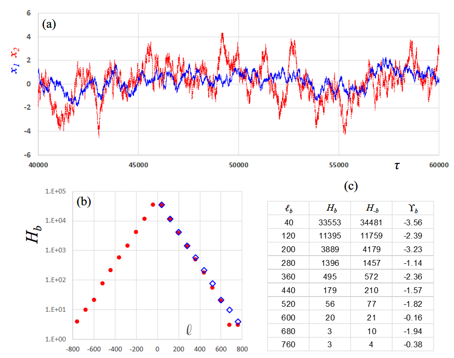
Figure 1: Simulation of coupled SHO’s in contact with two thermal baths. (a) A section of the time series (blue/red in contact with colder/hotter bath). (b) Histogram of $\ell$ ($H_{b}$). Blue diamonds are frequencies for bins with $\ell<0$, showing systematically higher values. (c) Table of center of bins (value of $\ell$) and frequencies $H_{\pm b}$, as well as the ratio $\Upsilon_{b}$ (see text for details).

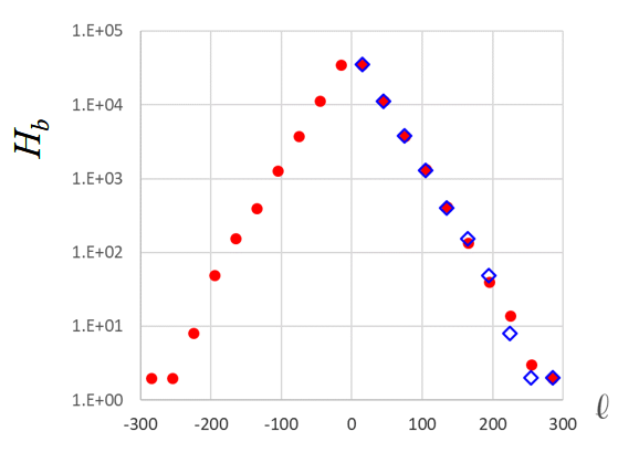
Figure 2: Histogram of $\ell$ ($H_{b}$) for a simulation of coupled SHO’s in contact with a single thermal bath. Blue diamonds are frequencies for bins with $\ell<0$, showing no systematic asymmetry.

As a contrast, we performed simulations for the same system coupled to a single thermal bath at $T=1$. Here, $\bar{\ell}\simeq-0.0155$ is considerably smaller, in comparison with $\sigma_{\ell}\simeq 38.4$. Meanwhile, Fig2 clearly shows there is no systematic asymmetry in the histogram. In addition to the signs of $\Upsilon$ being evenly distributed around zero, 70% of the $\left|\Upsilon\right|$’s are less than unity. We believe these two cases illustrate the import role played by the distribution of probability angular momentum for distinguishing whether a system is in a NESS or in thermal equilibrium (or so close that TRA is imperceptible).

IV.1.3 Linear Gaussian models

This subsection is devoted to a general class of systems, in which the TTSHO is a special case. Instead of just two variables, we consider any number of them ($\xi_{\alpha};~{}\alpha=1,...,N$), subjected to linearly restoring deterministic forces and additive Gaussian white noise ($\eta_{\alpha}$). Using a terminology common in climate science, we refer to these as “linear Gaussian models” (LGMs). Let us write the Langevin and Fokker-Planck equations as, respectively,

$$\partial_{t}\xi_{\alpha}=-F_{\alpha}^{\beta}\xi_{\beta}+\eta_{\alpha};~{}~{}\left\langle\eta_{\alpha}\left(t\right)\eta_{\beta}\left(t^{\prime}\right)\right\rangle=2D_{\alpha\beta}\delta\left(t-t^{\prime}\right)$$ (28)

and

$$\partial_{t}P=\partial^{\alpha}\left[D_{\alpha\beta}\partial^{\beta}P+F_{\alpha}^{\beta}\xi_{\beta}P\right]=-\partial^{\alpha}\left(J_{FP}\right)_{\alpha}$$ (29)

Of course, both $D_{\alpha\beta}$ and $F_{\alpha}^{\beta}$ are real and $D$ is symmetric, while the eigenvalues of both have positive real parts. Note that DB is satisfied if and only if the Fokker-Planck current, $J_{FP}$, vanishes, i.e., iff $\left(D^{-1}\right)^{\alpha\gamma}F_{\gamma}^{\beta}$ is symmetric and positive definite (i.e., $\left(C^{-1}\right)^{\alpha\beta}$ below). Here, our focus is on general $D$’s and $F$’s which lead to DB violation.

Whether DB is violated or not, the stationary distribution is still a GaussianMLax60 ; JBW03 ; ZS07 :

$$P^{\ast}\propto\exp\left\{-\frac{1}{2}\xi_{\alpha}\left(C^{-1}\right)^{\alpha\beta}\xi_{\beta}\right\}$$ (30)

Here, $\left(C^{-1}\right)^{\alpha\beta}$ is the inverse of the covariance matrix $\left\langle\xi_{\alpha}\xi_{\beta}\right\rangle^{\ast}$ and can be obtained from $D,F$ either by solvingJBW03 a general version of Eqn.(26):

$$F_{\beta}^{\gamma}C_{\gamma\alpha}+F_{\alpha}^{\gamma}C_{\gamma\beta}=2D_{\alpha\beta}$$

or summing over the eigenvectors of $F$ ZS07 . Using the formalism developed (Eqns.(12-18)), we see that the generalization of (27),

$$\left\langle\mathcal{L}_{\alpha\beta}\right\rangle^{\ast}=\left\langle-\xi_{\alpha}F_{\beta}^{\gamma}\xi_{\gamma}+\xi_{\beta}F_{\alpha}^{\gamma}\xi_{\gamma}\right\rangle^{\ast}=F_{\alpha}^{\gamma}C_{\gamma\beta}-F_{\beta}^{\gamma}C_{\gamma\alpha}$$ (31)

is an anti-symmetric tensor (with $N\left(N-1\right)/2$ independent components). As above, we verify that $\left(J_{FP}^{\ast}\right)_{\alpha}=\frac{1}{2}\left\langle\mathcal{L}_{\alpha\beta}\right\rangle^{\ast}\partial^{\beta}P^{\ast}$ so that $\partial_{t}P^{\ast}$ indeed vanishes.

Next, let us turn to a study of the distribution $Q\left(\mathcal{L}\right)$. Deferring most details to Appendix C, we show only some key results here (focusing on a single specific pair $\alpha$-$\beta$). First, its Fourier transform, given by

$$\tilde{Q}\left(z\right)=\int\left[\exp iz\left(\xi_{\alpha}\partial_{t}\xi_{\beta}-\xi_{\beta}\partial_{t}\xi_{\alpha}\right)\right]P\left(\vec{\eta}\right)P^{\ast}\left(\vec{\xi}\right)d\vec{\eta}d\vec{\xi}$$

can be computed exactly, as the integrand is Gaussian. Using the notation of $\mathbb{D}$,$\mathbb{F}$, etc., we find $\tilde{Q}=\left[\det\mathbb{C}^{-1}/\det\mathbb{G}\right]^{1/2}$where $\mathbb{G=C}^{-1}+2iz\mathbb{XF}+\left(2z^{2}/\varepsilon\right)\mathbb{XDX}^{T}$ and $\mathbb{X}$ is an anti-symmetric matrix with element $X_{\left(\alpha\beta\right)}^{\mu\nu}=\delta_{\alpha}^{\mu}\delta_{\beta}^{v}-\delta_{\alpha}^{\nu}\delta_{\beta}^{\mu}$. Thus,

$$\tilde{Q}\left(z\right)=\left\{\det\left[\mathbb{I}+2iz\mathbb{CXF}+\left(2z^{2}/\varepsilon\right)\mathbb{CXDX}^{T}\right]\right\}^{-1/2}$$ (32)

But $\det\left[\mathbb{I}+\mathbb{M}\right]=1+Tr\mathbb{M}+...+\det\mathbb{M}$, so that the first two terms of the Taylor series for $\tilde{Q}^{\ast}$ are

$$\tilde{Q}\left(z\right)=1-izTr\mathbb{CXF}+...$$

The first is normalization of $Q\left(\mathcal{L}\right)$, while the second is the first moment, i.e., $-i\partial_{z}\tilde{Q}\left(0\right)=\int\mathcal{L}Q$. Verifying $Tr\mathbb{CXF}=-\left\langle\mathcal{L}_{\alpha\beta}\right\rangle^{\ast}$, we are confident that Eqn.(32) is correct. Proceeding, we find that the $\det$ in Eqn.(32) is a quartic polynomial (since $\mathbb{X}$ is rank 2), real in $iz$. The location of its zeros can be extracted and the inverse transform to $Q$ can be analyzed. The conclusion is that the decays of $Q$ for $\mathcal{L\rightarrow\pm\infty}$ are dominated by exponentials:

$$\ln Q\left(\mathcal{L}\right)\propto-\left|\mathcal{L}\right|$$

More crucially, the two slopes are different and accounts for both $\left\langle\mathcal{L}\right\rangle\neq 0$ and $Q\left(\mathcal{L}\right)-Q\left(-\mathcal{L}\right)$ being systematically non-zero.

To end this subsection on LGMs, we present an illustration that contrasts with the TTSHO in significant ways. In particular, amongst the different ways to violate DB (by specifying $\mathbb{F}$ and $\mathbb{D}$ so that $\mathbb{FD\neq DF}^{T}$), the TTSHO involves a real-symmetric $\mathbb{F}$ that does not commute with $\mathbb{D}$. Another class involves asymmetric $\mathbb{F}$’s with complex eigenvalues (with positive real parts). Without noise, such an $\mathbb{F}$ will bring the system to a stable focus, i.e., a spiral stable fixed point. With additive white noise, this condition is sufficient, but not necessary, for the stochastic system to settle into a NESS (details in Appendix D). Furthermore, unlike the TTSHO case, it is possible to reach highly asymmetric distributions with this class of LGMs.

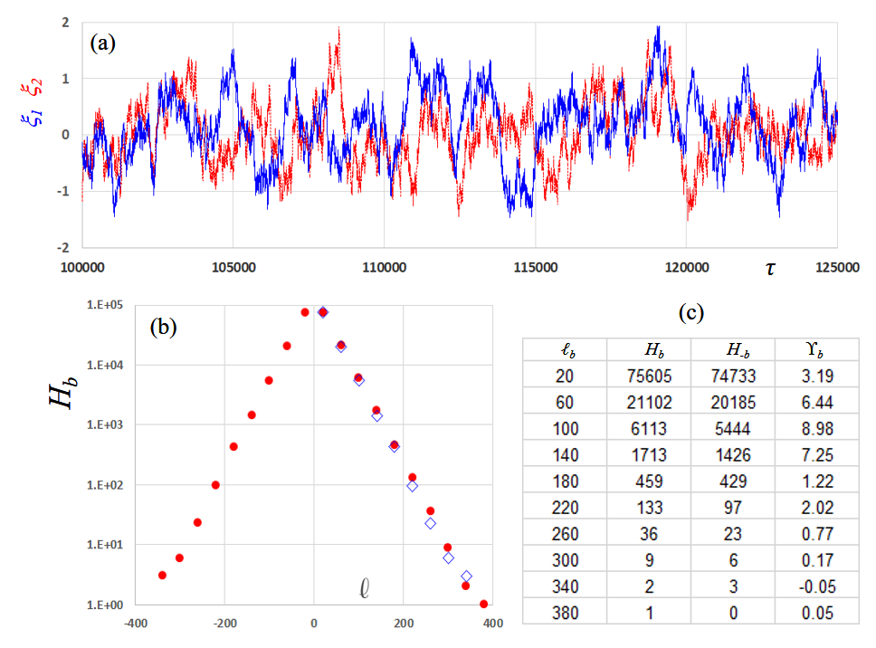
Figure 3: Simulation of an LGM with two degrees of freedom ($\xi_{1,2}$), driven by restoring linear forces with a spiral and subjected to additive white noise (which models a single thermal reservoir). (a) A section of the time series, showing no visually detectable signs of time reversal asymmetry. (b) Histogram of $\ell$ ($H_{b}$). Blue diamonds are frequencies for bins with $\ell<0$, showing systematically lower values. (c) Table of center of bins (value of $\ell$) and frequencies $H_{\pm b}$, as well as the ratio $\Upsilon_{b}$ (see text for details).

To illustrate these statements, we present here results from simulations of Eqn.(28), using methods detailed above, in a run of $200K$ steps with $\varepsilon=0.001$ for a $N=2$ system. Highlighting the non-trivial role played by $\mathbb{F}$ here, we choose

$$\mathbb{F}=\left(\begin{array}[c]{cc}2&1\\ -1&2\end{array}\right),~{}~{}\mathbb{D}=\left(\begin{array}[c]{cc}1&0\\ 0&1\end{array}\right)$$

In other words, this linearly driven system can be interpreted as one being coupled to a single thermal bath (at some unit $T$). Fig.3a shows a section of the time trace of this system in a stationary state, from which it is again unclear if TRA is present. Similarly, the trajectory in the $\xi_{1}$-$\xi_{2}$ plane also displays no perceptible rotation around the origin, as the noise masks the inward spiral due to $\mathbb{F}$. For this run, $\bar{\ell}$ $\simeq 0.935$, which is also quite small compared to $\sigma_{\ell}\simeq 43.9$. However, when we plot the histogram $H_{b}$, as shown in Fig.3b, we see that the counts for the $-\ell$ bins are systematically lower than those in the $+\ell$ ones. In Fig.3c, we show the bin centers $\ell_{\pm b}$, the frequencies $H_{\pm b}$, and $\Upsilon_{b}$. Again, we see that every $\Upsilon_{b}$ is positive and sizable (apart from one with $\left|\Upsilon_{b}\right|<1$, associated with a low count). On the theory front, we verify that $\mathbb{C=I}/2$, so that anti-symmetric part of $\mathbb{FC}$ gives us $A_{12}=0.5$ and so, $\left\langle\mathcal{L}\right\rangle^{\ast}=1$, a value comparable to the observed $\bar{\ell}$. Exploiting the techniques detailed in Appendix C, the asymptotic slopes of $\ln Q\left(\mathcal{L}\right)$ can also be computed and they are consistent with the decay in $H_{\pm b}$ shown in Fig.3c. Thus, we conclude that there is good agreement between simulation data and theoretical predictions.

IV.1.4 Example in one dimension: a biased random walker with reset

In this subsection, we focus on a NESS for a system with a one-dimensional variable, so as to illustrate the TRA signals discussed in subsection III.2. As in the previous cases, we will show results for both an equilibrium system and a NESS, so that some comparisons can be made. The model here is possibly the simplest version of a random walker with reset – a class of problems which gained considerable attention in recent yearsSatyaReset .

Our walker moves on non-negative integer sites along a line: $i=0,1,...$ in discrete time steps. At each step, it moves either one site higher (with probability $p$) or ‘resets’ to the origin:

$$R\left(i+1|i\right)=p;~{}~{}R\left(0|i\right)=1-p$$

It is trivial to see that, at large times, the system settles into the stationary distribution $P^{\ast}\left(i\right)=p^{i}\left(1-p\right)$. Note that this is identical to the $P^{\ast}$ for a particle in thermal equilibrium, hopping in a “gravitational field” with a impenetrable floor at $0_{-}$. All we need to arrive at that equilibrium state is to impose DB satisfying rates, i.e., the ratio for hopping “up one rung” to hopping “down a rung”, $R\left(i\rightarrow i+1\right)/R\left(i\rightarrow i-1\right)$, to be $p$.

Meanwhile, DB violation in our NESS is clear, as the persistent net currents are

$$K^{\ast}\left(i+1|i\right)=p^{i+1}/\left(1-p\right);~{}~{}K^{\ast}\left(0|i\right)=p^{i}$$

and satisfy $K^{\ast}\left(i+1|i\right)=K^{\ast}\left(0|i\right)+K^{\ast}\left(i|i-1\right)$ for $i>0$ and $K^{\ast}\left(1|0\right)=\sum_{i>0}K^{\ast}\left(0|i\right)$. There are many non-trivial current loops, of course, all of the form $0\rightarrow 1\rightarrow...\rightarrow m\rightarrow 0$. with $m>1$. The TRA generated can be detected by studying $\tilde{\Gamma}$ introduced in Eqn.(25). Here, $\zeta$ is the set of non-negative integers, $i$, and the simplest illustration for $\tilde{\Gamma}$ is the single time step case: $\upsilon=1$. Then, $P\left(j,1|i,0\right)P^{\ast}\left(i\right)$ reduces to

$$R\left(j|i\right)P^{\ast}\left(i\right) =\left[p\delta(j,i+1)+\left(1-p\right)\delta(j,0)\right]P^{\ast}\left(i\right)$$

$$=\left[p\delta(j,i+1)+\left(1-p\right)\delta(j,0)\right]p^{i}\left(1-p\right)$$

while the integral reduces to the sum

$$\sum_{i,j}ji\left(j-i\right)P\left(j,1|i,0\right)P^{\ast}\left(i\right)=\sum_{i=1}\left(i+1\right)ip^{i+1}\left(1-p\right)$$

The result is readily obtained:

$$\tilde{\Gamma}\left(1\right)=2\left(\frac{p}{1-p}\right)^{2}$$

Meanwhile, the standard deviation is $\sigma_{\zeta}=\sqrt{p}/\left(1-p\right)$, so that the dimensionless measure is

$$\tilde{\Gamma}/\sigma_{\zeta}^{3}=2\sqrt{p}\left(1-p\right)$$

the maximum of which occurs at $p=1/3$.

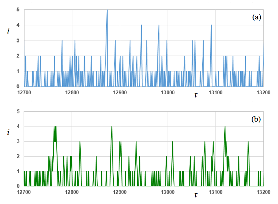
Figure 4: The time series for (a) a random walker with reset ($p=1/3$) in the steady state. Over the $500$ steps shown, it is discernibly asymmetric under time reversal. See text for the values of the mean position, its variance, the asymmetry $\tilde{\Gamma}$, and the ratio $\tilde{\Gamma}/\sigma_{\zeta}^{3}$ (over this run of $50K$ steps). By contrast, (b) shows a walker stepping up and down with probability ${\frac{1}{4}}$ and ${\frac{3}{4}}$, respectively, in a time symmetric equilibrium state. Note that both walkers have the same $P^{\ast}$, as hinted by these traces.

Simple simulations of this process provides excellent agreement with these predictions. For example, Fig.4a illustrates a part of the time trace, $i\left(\tau\right)$, in a run with just $50K$ steps with $p=1/3$. For this run, the comparison between data and theoretical predictions for various quantities (mean $\bar{\zeta}$, SD $\sigma_{\zeta}$, asymmetry $\tilde{\Gamma}$, and ratio $\tilde{\Gamma}/\sigma_{\zeta}^{3}$) are shown:

	$~{}~{}~{}~{}\bar{\zeta}$	$\sigma_{\zeta}$	$~{}~{}~{}~{}\tilde{\Gamma}$	$\tilde{\Gamma}/\sigma_{\zeta}^{3}$
Simulations	$0.5002$	$0.8658$	$0.4996$	$0.7698$
Theory	$0.5000$	$0.8660$	$0.5000$	$0.7698$

So we conclude that the agreement is excellent and TRA is clear. As a contrast, in a similar run with DB satisfying rates (Fig.4b, with specifically $R\left(i\rightarrow i+1\right)=p/\left(1+p\right)$ and $R\left(i\rightarrow i-1\right)=1/\left(1+p\right)$ ), the asymmetry is found to be zero, while the average and variance are entirely consistent with theoretical values. To emphasize, the stationary $P^{\ast}\left(i\right)$ for both systems are identical. There are non-trivial current loops in the NESS, as measured by $\tilde{\Gamma}$, but none in the equilibrium system. Visually, it is possible to discern the difference (in TRA) between these two time traces. Of course, the NESS in this example is quite extreme. If a combination of these two dynamics were introduced (i.e., with a fraction of the updates being DB violating), then it may be quite difficult to distinguish a system “slightly perturbed from equilibrium” than one truly in equilibrium.

IV.2 From the subtle to the manifest

All of the examples studied above are solvable exactly. In this sense, they may be regarded as “toy models” rather than realistic ones designed for systems in nature, where non-linearities abound. In general, the latter are not analytically accessible, so that information about how they display TRA is typically gleaned from simulations. Of course, we can also study data collected from physical systems directly, such as those under controlled environments in laboratories or observed in complex natural settings (from micro to global, in e.g., biological and climate sciencesBBF16 ; WFMNZ21 ). In nearly all such systems, it is the exception that the underlying dynamics obey DB and the steady states fall within equilibrium statistical mechanics. While some of these NESS are “close” to equilibrium and display subtle signals of TRA, others are clearly “far from” equilibrium and TRA is manifest. In this subsection, we illustrate this wide spectrum of possibilities with examples from both physical data and numerical simulations.

IV.2.1 Illustrations from two climate systems

Let us begin with two illustrations of TRA published recentlyWFMNZ21 , based on data from our climate. Both display somewhat “subtle” asymmetry under time reversal, in that one shows $\bar{\ell}<\sigma_{\ell}$ while the other, $\bar{\ell}\simeq\sigma_{\ell}$. The former is associated with the well-known phenomenon of El-Niño and the latter, with the Madden-Julien Oscillation. Both are considerably further from equilibrium than the simple examples shown above (where $\bar{\ell}\ll\sigma_{\ell}$).

El-Niño is generally associated with the warming of the tropical Pacific Ocean. A less well-known feature is the variations of the depth of the thermocline. While there are many ways to characterize “warming” and “depth,” we focus on two common measures of these features:

• NINO3, the sea surface temperature averaged over a certain region in the eastern Pacific (in units of ${}^{\circ}C$)

• d20, the depth of the $20^{\circ}C$ isotherm in the tropical Pacific (in units of $cm$).

Details of these measures and the data sets chosen may be found in Ref. WFMNZ21 . The time series of these quantities consist of monthly averages of observations from 1960 to 2016. Setting the means of these series to zero, we work with the “anomalies” of NINO3 and d20. When the entire trajectory is plotted in the NINO3-d20 plane, there is no obvious systematic rotation around the origin. In Fig.5b, we illustrate with a small section, which may give an impression of a tendency to rotate clockwise. When we compute $\bar{\ell}$ and $\sigma_{\ell}$, we find $-205.0$ and $432.4$ (in units of ${}^{\circ}C$-$cm/month$), respectively. Since $\bar{\ell}$ is just half of $\sigma_{\ell}$, we compile the histogram of $\ell$’s and display it (colored as blue columns) in Fig.5a. There is a clear asymmetry in favor of negative $\bar{\ell}$ bins. Similarly, in Figs. 5c and d, we show the distribution and a sample trajectory for the two dominant amplitudes associated with the Madden-Julien Oscillation. Here, the asymmetry is much more prominent in both representations, a result consistent with $\bar{\ell}$ being comparable to $\sigma_{\ell}$, namely, $0.201$ and $0.263$, respectively (in units of $amplitude^{2}/day$).

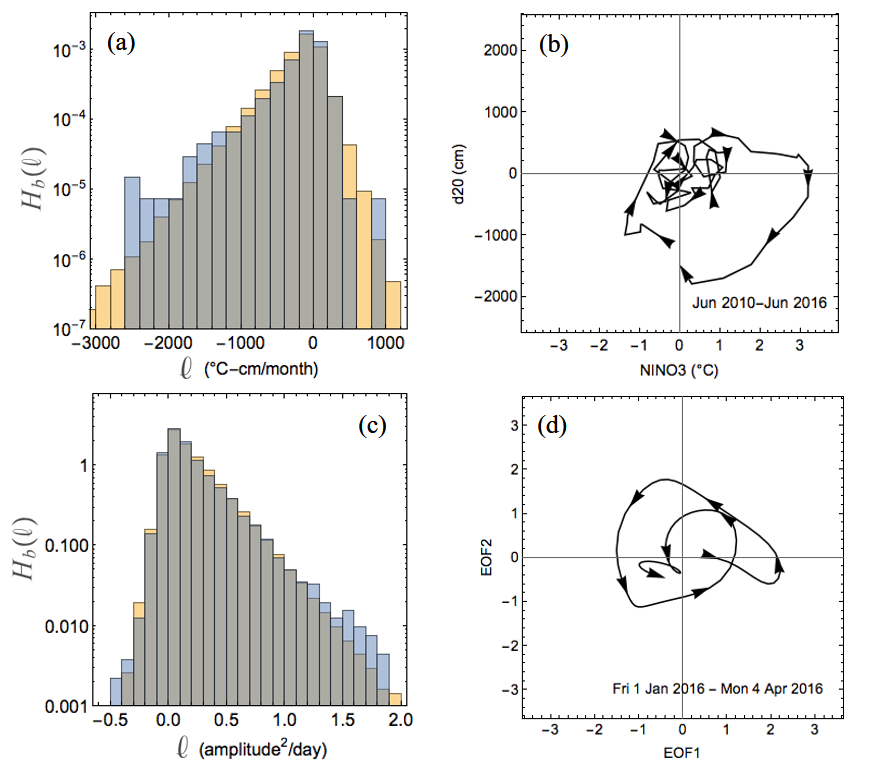
Figure 5: Histograms/distributions of $\ell$ and trajectories for a pair of quantities associated with El-Niño (a,b) and Madden-Julien Oscillations (c,d). In (a,c), blue bars represent data, orange ones represent theory, and grey is for regions of overlapping blue/orange. See text for details. (Figures reproduced from Ref.WFMNZ21 .)

On the theory front, parameters for LGMs were chosen to fit the time-series. (See Appendix E for further details.) In turn, these models predict values for $\bar{\ell}$ and $\sigma_{\ell}$ and, correponding to the above cases, they are $-205.7$, $350.7$, $0.199$, and $0.250$. All predictions are in acceptable agreement with data. The distributions $Q$ can be computed by inverting $\tilde{Q}$ numerically. The resultant are plotted as orange columns in the histogram figures ($H_{b}$). Meanwhile, the grey regions in the columns represent the overlap of theory and data. From these, we conclude that the LGMs have captured the essentials of the asymmetry in $H_{b}$ (and $Q\left(\mathcal{L}\right)$), and they provide good approximants for the non-equilibrium quasi-stationary states in nature. Finally, let us highlight the fact that the LGMs for both systems belong to the class of $\mathbb{F}$’s with stable focus. Unlike the model system presented in Section IV.1.3, the twists (i.e., antisymmetric parts of $\mathbb{F}$) are progressively stronger (from El-Niño to MJO). The underlying physics here is entirely consistent with the increase in both the ratio $\bar{\ell}/\sigma_{\ell}$ and the prominence of the asymmetry in the $H_{b}$ plots.

IV.2.2 Hopf bifurcation and transition from subtle to manifest display of TRA

While the climate data we presented represent a significant increase of the TRA signal from that in the TTSHO, say, we may still regard them as borderline cases in the “subtle-manifest” spectrum. The next level of asymmetry is so prominent that it deserves the term “manifest,” namely, when the system undergoes a Hopf bifurcationHopf43 and displays limit cycles which are unmistakably irreversible in time. In nature, such phenomena are abundant – in quasi-stationary cyclic states rather than truly stationary ones – from predator-prey systems to chemical reactions. To explore bona-fide stationary stochastics processes, we turn to model systems inspired by various natural phenomena. In this subsection, we follow this route, in order to illustrate the effects of such a transition on $\left\langle\mathcal{L}\right\rangle$ and its distribution. Naturally, we must go beyond the LGM and so, typically, few exact analytic results are known and simulations offer the best progress for most model systems. By exploiting a sufficiently simple model for a stochastic (supercritical) Hopf bifurcation, we can present some exact results (stationary distribution $P^{\ast}$ and current $\vec{J}_{FP}^{\ast}=\vec{\mu}P^{\ast}-D\vec{\nabla}P^{\ast}$) as well as some visually appealing simulation data.

Here again, our model consists of two variables ($\xi_{1,2}$), forced by a conservative part ($-\vec{\nabla}V$) plus a twist ($\vec{F}_{\omega}\propto\omega$), and subjected to a trivial $\vec{\eta}$ ($\mathbb{D}=T\mathbb{I}$). Defining $r^{2}\equiv\xi_{1}^{2}+\xi_{2}^{2}$, we choose a standard potential

$$V\left(\xi_{1},\xi_{2}\right)=\frac{\rho}{2}r^{2}+\frac{u}{4}r^{4}$$

which allows a Hopf bifurcation, at $\rho=0$. Without the twist, the system settles into thermal equilibrium of course (with $P^{\ast}\propto e^{-V/T};$ $k_{B}=1$) and is often used to model, say, a system of classical spins. For $\rho>0$, it is “above the critical temperature” where the rotational symmetry is unbroken. When $\rho$ turns negative, we have spontaneous symmetry breaking, with the minimum energy state given by $r=\sqrt{-\rho/u}$. If a twist

$$\vec{F}_{\omega}=\left(\begin{array}[c]{cc}0&\omega\\ -\omega&0\end{array}\right)\vec{\xi}$$

is added, then the stochastic system, specified by the Langevin equation,

$$\partial_{t}\vec{\xi}=-\vec{\nabla}V-\vec{F}_{\omega}+\vec{\eta}$$

will tend to “jiggle” near the origin $\vec{\xi}=\vec{0}$ in case $\rho>0$ (similar to the example shown in Fig.3). But, for $\rho<0$ (with large $-\rho/u$ and small $T$), the trajectories will be mostly circular with small deviations. We may refer to such cases as limit cycles with low noise. Near the transition, i.e., small $-\rho/u,\omega$ and moderate $T$, TRA signals from the system will undoubtedly be “subtle”. Deep into the broken-symmetry and twist-driven region, i.e., large $-\rho/u,\omega$ and small $T$, the signal should be “manifest”. In this toy model, it is straightforward to show that, for the Fokker-Planck equation

$$\partial_{t}P=-\vec{\nabla}\cdot\vec{J}_{FP}=\vec{\nabla}\cdot\left[\left(\vec{\nabla}V+\vec{F}_{\omega}\right)P+T\vec{\nabla}P\right]$$

the stationary distribution is simply $P^{\ast}\propto e^{-V/T}$ (since both $\vec{\nabla}\cdot\vec{F}_{\omega}$ and $\vec{F}_{\omega}\cdot\vec{\nabla}V$ vanish), with $\vec{J}_{FP}^{\ast}=-\vec{F}_{\omega}P^{\ast}$. From here, quantities such as $\left\langle\mathcal{L}\right\rangle^{\ast},\sigma_{\mathcal{L}},Q^{\ast}\left(\mathcal{L}\right)$ can be computed numerically, as none of the integrands are simple Gaussians.

Our main interest here is to illustrate the qualitative features of this stochastic process and how they differ from those in the LGMs. Thus, we will present only a figure of a simulation of the above system and highlight the differences, while avoiding technical details. As in previous simulations, we carried out a run of $200K$ steps with $\varepsilon=0.001$ with $\rho=u=\omega=1$ and $T=0.1$.

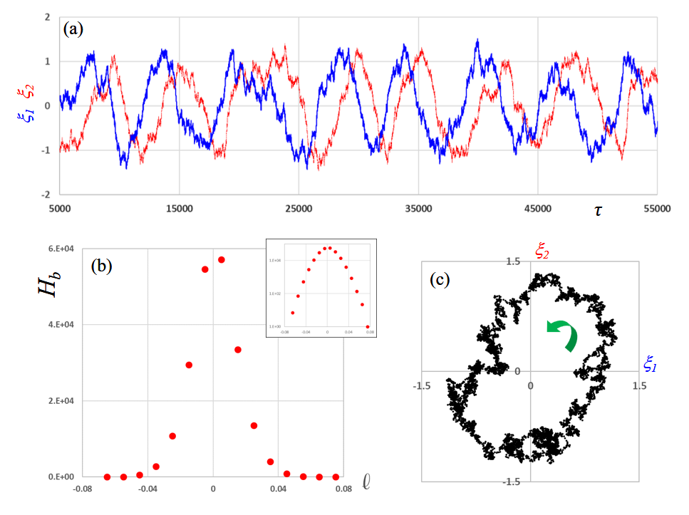
Figure 6: Simulation of a system with two degrees of freedom ($\xi_{1,2}$), driven into a limit cycle by deterministic forces and subjected to additive white noise (which models a single thermal reservoir). (a) A section of the time series, displaying prominent signs of time reversal asymmetry. (b) Histogram of $\ell$ ($H_{b}$). The asymmetry between positive and negative bins is quite clear. In the inset is a log plot, showing the distribution is closer to Gaussian rather than (double) exponential. (c) A section of the trajectory in the $\xi_{1}$-$\xi_{2}$ plane, with the green arrow indicating the direction of motion.

Fig. 6a shows a section of the time trace of this system in a stationary state, from which it is quite clear that TRA is present. For example, it is qualitatively similar to a predator-prey system, in which a rise of the predator population ($\xi_{2}$, red trace) soon follows a rise in the prey numbers ($\xi_{1}$, blue trace). Similarly, the trajectory in the $\xi_{1}$-$\xi_{2}$ plane displays an obvious direction of motion, as indicated by the green arrow. Despite the clear sense of rotation in this run, the presence of angular momentum is not prominent, as its typical values are dominated by the noise in $\partial_{t}\vec{\xi}$. As a result, $\bar{\ell}$ $\simeq 1.00$ is relatively small compared to $\sigma_{\ell}\simeq 14.3$. While the histogram $H_{b}$ in Fig.6b is certainly biased in favor of $\ell>0$, the asymmetry is overwhelmed by the width of the distribution. More interesting is the inset figure, showing that $H_{b}$ is no longer exponential at large $\ell$. Instead, it is essentially Gaussian, so that its make-up can be interpreted readily: a noise dominated Gaussian part, displaced by a small positive mean ($\bar{\ell}>0$). Not surprisingly, when $T$ is lowered by a factor of $100$, say, $\sigma_{\ell}$ drops by a factor of $10$, while $\bar{\ell}$ remains essentially unchanged. The stationary distribution ($P^{\ast}$, not displayed explicitly) is quite distinct from the LGM case above. Instead of a single peaked Gaussian, it resembles a volcano, with a dip at the center and a rim (circular in this simple model) at $r=1$. There is a non-trivial, persistent probability current moving around this structure, contributing to a non-vanishing $\left\langle\mathcal{L}\right\rangle^{\ast}$. It is reasonable to conclude that, when a stochastic process settles into a (noisy) limit cycle, DB and time reversal violation will be “manifest.”

IV.3 Astonishing complex behavior from minimal models in nonequilibrium steady states

The simple solvable examples above should not give the reader the impression that NESS is well understood. On the contrary, a casual glance around us provides an astounding array of phenomena which we cannot predict from their microscopic constituents (and interactions), e.g., all forms of life. Even much simpler systems, such as point particles diffusing on a lattice under DB violating rules, can pose serious challenges. Known as driven diffusive systems, they have been the focus of research since the 1980’sSZ95 . Arguably the simplest of these is the well-established Ising lattice gasYL52 driven far from equilibriumKLS84 . It displays many intriguing properties, some of which are yet to be understood. Here, we present another “minimal model” – the lattice gas versionDS95 of the Widom-Rowlinson modelWR70 – easily understood if subjected to equilibrium conditions. However, when driven uniformly out of equilibrium (e.g., biased diffusion in one direction, say), the system displays remarkably surprising and complex behaviorDZ18 ; LDZ21 . In this subsection, we present only a brief summary, so as to illustrate how seemingly trivial changes of the dynamics (from DB satisfying to violating) can lead to profound changes in the collective behavior of a statistical system.

Introduced in 1995, the Widom-Rowlinson lattice gas (WRLG) DS95 consists of two species of particle (say, A and B) placed singly on a square lattice (or other lattices, in other dimensions), diffusing freely via nearest neighbor particle-hole exchange. Configurations are specified by $\left\{s\left(\vec{x}\right)\right\};s=\pm 1,0$ representing site $\vec{x}$ being occupied by A,B, or vacant. The only other constraint is that AB nearest neighbor pairs are excluded. With no energy functional, temperature is irrelevant. The only control parameters are the densities of the two species. In other words, entropy is the sole key for this equilibrium system (i.e., the microcanonical ensemble with $P^{\ast}\left(\mathcal{C}\right)\propto 1$ for any allowed $\mathcal{C}$). Since the NN-exclusion acts as an entropic force, we may expect an effective attraction between AA and BB pairs, as in a standard Ising lattice gas. This picture is mainly confirmed in simulation studies, most of which have equal numbers of A and B, with the overall density ($\bar{\rho}$) as a tunable parameter. As expected, the system is homogeneous for small $\bar{\rho}$, with a transition to a phase separated state (two regions: A-rich or B-rich, e.g., left panel in Fig.7) when the density exceeds a critical value: $\rho_{c}\simeq 0.617(1)$. Near $\rho_{c}$ the critical behavior is in the Ising universality classDS95 . Our interest here is when a bias is introduced into the particle-hole exchange so that DB is violated and the system settles into a NESS instead.

Unlike earlier studies of biased diffusion of two species, in which interesting phases were discovered when A and B are driven in opposite directionABC , both species are driven in the same direction in this system. Intuitively, it appears that a drive that does not distinguish the species should have little effect. Yet, completely unexpected properties were discovered through simulations, even when the system is in the disordered phase. We summarize some of these findings here.

If the single species, non-interacting Ising lattice gas is driven, the stationary distribution remains uninteresting ($P^{\ast}\propto 1$). For the driven WRLG in one dimension, it is clear that the same mechanism leads to $P^{\ast}\propto 1$. However, simulations in two dimensions (e.g., on square lattices of $L\times L$ sites, with toroidal BCs) show that $P^{\ast}$ is far from simple. Generically, in addition to displaying long range correlations (as in the KLS modelKLS84 ), the drive induces a preferred lengthDZ18 ; LDZ21 . In particular, even for $\bar{\rho}\ll 1$, the steady state structure factor (i.e., the Fourier transform of the two point equal-time correlation ($\left\langle s\left(\vec{x}\right)s\left(\vec{x}^{\prime}\right)\right\rangle^{\ast}$) in this homogeneous state does not assume the standard Ornstein-Zernike form. Instead, it peaks at a preferred, non-trivial wave-vector, $\vec{q}$, parallel to the drive direction. Correspondingly, $\left\langle s\left(\vec{x}\right)s\left(\vec{x}^{\prime}\right)\right\rangle^{\ast}$ does not decay exponentially for large $\left|\vec{x}-\vec{x}^{\prime}\right|$, but oscillates much like a damped spring, with wavelength $\Lambda\equiv 2\pi/\left|\vec{q}\right|$. For $\bar{\rho}=0.5$, $\left|\vec{q}\right|$ rises more or less linearly with the strength of the driveLDZ21 . For fixed drive and increasing $\bar{\rho}$, $\vec{q}$ also increases, but only slightly. Meanwhile, the value at the peak rises substantially with higher $\bar{\rho}$, until a critical $\bar{\rho}_{c}$ is reached. Beyond $\bar{\rho}_{c}$, the peak height scales with system size rather than being intensive – a characteristic of long range order and phase separation. Unlike the undriven case, where the system always ordered into two particle-rich regions (similar to the Ising case, i.e., $\Lambda=L$), the driven WRLG displays lamellae normal to the drive, with a fixed width – an $L$-independent $\Lambda/2$. To illustrate, we show two typical configurations with $\rho=0.7$ in Fig.7, one in equilibrium and the other, a driven system.

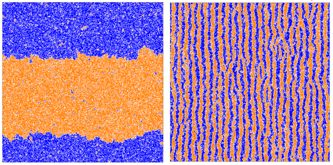
Figure 7: Typical configurations for the Widom-Rowlinson lattice gas (left panel) and the driven version (right panel, with particles biased $3\times$ more to move to the right than to the left). Blue and orange sites are occupied by equal numbers of the two species of particles. Vacancies are shown as white. Both systems are $400\times 400$ with $\bar{\rho}=0.7$. (Figures reproduced from Ref.LDZ21 .)

Further, $\Lambda$ varies in a very perplexing manner. To emphasize, this lamellae structure is present even in the homogeneous phase with a small drive (though difficult to discern). For maximal drive, $10\lesssim\Lambda\lesssim 12$ (lattice spacings, deduced from the correlation function) deep within this phase ($\bar{\rho}\sim 0.4$). Around $\bar{\rho}_{c}\sim 0.77$, ordering emerges and the lamellae appear as “visible strips” (in square lattices). As $\bar{\rho}$ increases further, $\Lambda$ rises by minute amounts and remains $L$ independent. In other words, in these regime, $\Lambda$ appears to be a characteristic of the microscopic parameters, so that the number of strips is essentially $L/\Lambda$. As $\bar{\rho}_{c}$ closes on unity, this number decreases rapidly, via a series of “strip-merging” transitions. The boundary of this regime, $\bar{\rho}_{sm}$, is likely to depend on $L$ in a complicated manner. Eventually ($\bar{\rho}\lesssim 1-2/L$, clearly), the system ends in a completely phase segregated state: $\Lambda=L$, with one strip of each species, separated by thin ($\sim$ lattice spacing) strips of holes. In simulations involving $L\leq 400$, strip-merging appears for $\bar{\rho}>\bar{\rho}_{sm}\sim 0.9$. For other values of the bias, the behavior of $\Lambda,\bar{\rho}_{c},\bar{\rho}_{sm}$ on $\bar{\rho}$ is highly non-trivial DZ18 ; LDZ21 and remains to be explored in detail. In all cases, $\Lambda$ rises to $O\left(L\right)$ at both extremes of $\bar{\rho}$.

The driven WRLG provides a good example of a stationary state which is clearly far from having the maximal entropy (disorder). No one could have predicted the emergence of the lamellae structures from the simple transition rates (translation invariant in both space and time) in this minimal system. Although we did not discuss TRA explicitly in this case, the drift of particles is so clear that showing TRA by some other means seems redundant. What needs to be emphasized here is the DB violation is undeniably at play, as the steady state display phenomena which are far from being consistent with maximal entropy. In many ways, the surprises here are in the same class as those found in, say, Conway’s game of lifeConway , in which complex patterns emerge from minimal rules and constituents. We believe that, beyond simple signals of time reversal asymmetry, this aspect of non-equilibrium statistical mechanics – the emergence of complexity from simplicity – will be a rewarding and exciting frontier for future investigations into the mysteries of cooperative phenomena.

V Summary and Outlook

When a statistical system settles into its stationary state, time translational invariance holds, by definition. However, this state may or may not be symmetric under time reversal, depending on whether the system is in thermal equilibrium or a non-equilibrium steady state. In layman’s terms, snap shots of a movie at different times – of either steady states – will appear statistically the same, but there may be a difference when the movies are run forwards vs. backwards. The origin of the difference lies in whether the rules for evolution of the system obeys detailed balance or not. This article is devoted to simple ways to detect asymmetries under time reversal.

In general, to observe time dependence phenomena, we need correlations at unequal times. Here, we presented the simplest of such functions to detect TRA, relying on the most elementary of observables and the minimal separation of just two times. In elementary physics, these observables can be positions of particles ($\vec{x}$) while “minimal time separation” can be $\delta t$. Meanwhile, the velocity $\vec{v}=\delta\vec{x}/\delta t$ is the simplest quantity odd under time reversal. To study the statistical properties of systems in steady states, we turn to averages (means and correlations), denoted by $\left\langle...\right\rangle^{\ast}$. But $\left\langle\vec{x}\right\rangle^{\ast}=\left\langle\vec{v}\right\rangle^{\ast}\equiv 0$, and to detect time reversal asymmetry, nothing is simpler than the averages of their product. Of course, $\left\langle\vec{x}\cdot\vec{v}\right\rangle^{\ast}=$ $\frac{1}{2}\left\langle\partial_{t}x^{2}\right\rangle^{\ast}\equiv 0$, and we are naturally led to consider $\left\langle\vec{x}\times\vec{v}\right\rangle^{\ast}$ (or $\left\langle\xi_{\alpha}\Delta\xi_{\beta}-\xi_{\beta}\Delta\xi_{\alpha}\right\rangle^{\ast}$ in general). Recognizing $\vec{x}\times\vec{p}$ is angular momentum in elementary physics, we coin the term probability angular momentum ($\mathcal{L}$) for the correlation function introduced. If configuration space consists of just one dimension, then $\vec{x}\times\vec{p}\equiv 0$ and a different quantity (involving third moments) was proposed for detecting TRA.

Relating these abstract concepts to data (from simulations, experiments, or observations), we are aware that averages from finite data sets are almost never identically zero, so that using $\left\langle\mathcal{L}\right\rangle^{\ast}\neq 0$ as a test for TRA is too idealistic. Further, we find that comparing its magnitude to its standard deviation ($\sigma_{\mathcal{L}}$) rarely provides a reliable gauge. In particular, many model systems with built in DB violating dynamics display $\left\langle\mathcal{L}\right\rangle^{\ast}\ll\sigma_{\mathcal{L}}$. This issue motivated us to consider $Q\left(\mathcal{L}\right)$, the full distribution of $\mathcal{L}$. For many system, it is broadly spread around $\mathcal{L}=0$, while TRA manifests as an asymmetry: $Q\left(\mathcal{L}\right)\neq Q\left(-\mathcal{L}\right)$. In practice, time series of observables can be used to build histograms associated with $\mathcal{L}$, while we proposed a measure ($\Upsilon$) which appears to be quite reliable for deciding if a system displays TRA or not. We refer to systems with such signals of TRA as “subtle,” since there are no overt signs of time reversal imbalance. By contrast, many steady state systems in nature (or quasi-stationary states) display “manifest” signs of TRA, especially those with limit cycles. At the far end of this subtle-manifest continuum are stochastic processes which display phenomena well beyond our knowledge or expectations: Discoveries of new species of life forms continue to astonish us. Even seemingly trivial constituents evolving with simple rules can lead to unpredictably complex behavior, e.g., Conway’s game of life. Driven diffusive systemsSZ95 provide another good example, as we learn that collective phenomena in stochastic processes evolving with DB violating dynamics can be extremely rich and surprising. To illustrate these ideas, a number of examples were presented, from simple solvable systems to complex physical ones.

The limited study here should be regarded as a small glimpse into the wide vistas of NESS. Specifically, our explorations naturally raised more questions. In addition to the ones noted in the text, we list a few other examples here. (i) The simplest of observables for detecting TRA is considered here, as $\mathcal{L}$ is a two point correlation at “one time step” apart, though $Q\left(\mathcal{L}\right)$ effectively involve all its higher moments. One generalization we did not study is correlations involving larger separations of times, e.g., $\mathcal{A}_{\alpha\beta}\left(\tau\right)\equiv~{}\left\langle\xi_{\alpha}\left(\tau\right)\xi_{\beta}\left(0\right)-\xi_{\beta}\left(\tau\right)\xi_{\alpha}\left(0\right)\right\rangle^{\ast}$ with any $\tau$. Since most correlations decay with time, we expect each term of $\mathcal{A}$ to vanish for large $\tau$. Yet, there are situations where it may increase with $\tau$ up to some maximum at $\hat{\tau}$, before decayingShrZ14 . Not only would $\mathcal{A}_{\alpha\beta}\left(\hat{\tau}\right)$ provide a more prominent signal of TRA than $\mathcal{L}$, it points to the presence of a characteristic time scale. The implications of $\hat{\tau}$ for systems with “subtle” signals are clearly worthy of pursuit. (ii) We noted that $Q\left(\mathcal{L}\right)$ undergoes a transition from an asymmetric Laplacian-like distribution (with exponential decays) to an approximate Gaussian (with zero mean) as the system makes a Hopf bifurcation. How does the linear behavior in $\ln Q$ crossover to the quadratic? via anomalous exponents or at some crossover value $\ell_{\times}$? If the latter, how does it vary with critical control parameter(s)? For simplicity, we presented cases with just two variables. Would a “many-body” system provide us with further, unexpected collective behaviour? (iii) We showed that $\mathcal{L}$ (and $\tilde{\Gamma}$ for more restrictive systems) serves as an effective measure for detecting TRA in simple model systems. Beyond these immediate questions, does this line of inquiry lead to any new insights for other NESS in complex systems in nature, such as those in chemical reactions, biological sciences, socio-economic arenas, global ecology/climate, and stellar interiors? Most crucially, our hope is that it provides an inroad into formulating an overarching framework for statistical mechanics of non-equilibrium steady states.

Appendix A Decomposition of $\left\langle\xi_{\alpha}v_{\beta}\right\rangle^{\ast}$

In the steady state, $\left\langle\xi_{\alpha}\xi_{\beta}\right\rangle^{\ast}$ at one time is the same as at an infinitesimal time later (when each $\xi$ changes by $\varepsilon\partial_{t}\xi=\varepsilon v$). Let us write this statement as

$$\left\langle\xi_{\alpha}\xi_{\beta}\right\rangle^{\ast}=\left\langle\left(\xi_{\alpha}+\varepsilon v_{\alpha}\right)\left(\xi_{\beta}+\varepsilon v_{\beta}\right)\right\rangle^{\ast}$$ (33)

Using the Langevin representation, we have

$$v_{\alpha}=\mu_{\alpha}+\eta_{\alpha}$$

where

$$\left\langle\eta_{\alpha}\right\rangle=0;~{}~{}\left\langle\eta_{\alpha}\eta_{\beta}\right\rangle=2D_{\alpha\beta}\frac{1}{\varepsilon}$$

with $1/\varepsilon$ representing $\delta$ in $\left\langle\eta_{\alpha}\eta_{\beta}\right\rangle\propto\delta\left(t-t^{\prime}\right)$. In the the limit of $\varepsilon\rightarrow 0$, we find from (33)

$$\left\langle\xi_{\alpha}v_{\beta}+v_{\alpha}\xi_{\beta}\right\rangle^{\ast}=-\varepsilon\left\langle\eta_{\alpha}\eta_{\beta}\right\rangle=-2D_{\alpha\beta}$$

Here, we verify that the units of both sides are indeed $\left[\xi_{\alpha}\right]\left[\xi_{\beta}\right]\left[t\right]^{-1}$. Meanwhile, by definition, we have

$$\left\langle\xi_{\alpha}v_{\beta}-v_{\alpha}\xi_{\beta}\right\rangle^{\ast}=\mathcal{L}_{\alpha\beta}$$

Defining

$$A_{\alpha\beta}\equiv\mathcal{L}_{\alpha\beta}/2$$

we see that it is precisely the rate of “area” (in the $\alpha$-$\beta$ plane) being swept out. Then, $\left\langle\xi_{\alpha}v_{\beta}\right\rangle^{\ast}$ can be decomposed to a symmetric part ($-D$) and an anti-symmetric one ($A$):

$$\left\langle\xi_{\alpha}v_{\beta}\right\rangle^{\ast}=-D_{\alpha\beta}+A_{\alpha\beta}$$

In this sense, we regard the probability angular momentum to be on the same footing as the diffusion coefficients. Finally, since $\left\langle\eta\right\rangle=0$, we can also write the decomposition as $\left\langle\xi_{\alpha}\mu_{\beta}\right\rangle^{\ast}=-D_{\alpha\beta}+A_{\alpha\beta}$. For LGMs, $\mu_{\beta}=-F_{\beta}^{\gamma}\xi_{\gamma}$, so that we end up with $F_{\beta}^{\gamma}C_{\gamma\alpha}=D_{\alpha\beta}-A_{\alpha\beta}$, where $C_{\gamma\alpha}=\left\langle\xi_{\alpha}\xi_{\gamma}\right\rangle^{\ast}$. Since $D$ is symmetric, we can summarize neatly

$$F_{\alpha}^{\gamma}C_{\gamma\beta}=D_{\alpha\beta}+A_{\alpha\beta}$$ (34)

Appendix B A Simple 3-state system in NESS

Here we include some details of the system with $i=1,2,3$ configurations (“micro-states”) presented in subsection IV.1.1. Writing the probabilities to find the system in $i$ at discrete time $\tau$ as a column vector,

$$\left|P\right\rangle\equiv\left(\begin{array}[c]{c}P\left(1,\tau\right)\\ P\left(2,\tau\right)\\ P\left(3,\tau\right)\end{array}\right)$$

the Master equation reads

$$\Delta_{\tau}\left|P\right\rangle=\mathfrak{L}\left|P\right\rangle$$

where

$$\mathfrak{L}=\left(\begin{array}[c]{ccc}-\varphi-\tilde{\varphi}&1&1\\ \varphi&-1-\varphi&1\\ \tilde{\varphi}&\varphi&-2\end{array}\right)$$

Conservation of probability is $\sum_{i}P\left(i,\tau\right)=1$, consistent with $\left\langle w_{0}\right|\equiv\left(\begin{array}[c]{ccc}1&1&1\end{array}\right)$ being a left eigenvector of $\mathfrak{L}$ with zero eigenvalue: $\omega_{0}=0$. The associated right eigenvector is the stationary distribution:

$$\left|P^{\ast}\right\rangle\equiv\left|u_{0}\right\rangle=\frac{1}{Z}\left(\begin{array}[c]{c}2+\varphi\\ 2\varphi+\tilde{\varphi}\\ \varphi^{2}+\tilde{\varphi}\varphi+\tilde{\varphi}\end{array}\right)$$

where $Z=\left(2+\varphi\right)\left(1+\varphi+\tilde{\varphi}\right)$. The other two ($n=1,2$) left and right eigenvectors are

$$\left\langle w_{n}\right| =\left(\begin{array}[c]{ccc}\varphi+\tilde{\varphi}&-1&-1\end{array}\right),~{}~{}\left(\begin{array}[c]{ccc}\tilde{\varphi}-\varphi^{2}&2\varphi-\varphi\tilde{\varphi}-\tilde{\varphi}&\varphi+\tilde{\varphi}-2\end{array}\right)$$

$$\left|u_{n}\right\rangle =\left(\begin{array}[c]{c}\tilde{\varphi}-1\\ -\left(1+\varphi\right)\\ \varphi-\tilde{\varphi}\end{array}\right),~{}~{}\left(\begin{array}[c]{c}0\\ 1\\ -1\end{array}\right)$$

associated with the eigenvalues:

$$\omega_{n}=-\left(1+\varphi+\tilde{\varphi}\right),~{}~{}-\left(2+\varphi\right)$$

As a result, for such a simple system, we can provide the full, time dependent, solution to our system:

$$\left|P\right\rangle =\left(\mathfrak{I}+\mathfrak{L}\right)^{\tau/\varepsilon}\left|P_{ini}\right\rangle$$

$$={\displaystyle\sum\limits_{n=0}^{2}}\left(1+\omega_{n}\right)^{t/\tau}\frac{\left\langle w_{n}\right|\left.P_{ini}\right\rangle}{\left\langle w_{n}\right|\left.u_{n}\right\rangle}\left|u_{n}\right\rangle$$

$$=\left|P^{\ast}\right\rangle+{\displaystyle\sum\limits_{n=1}^{2}}\left(1+\omega_{n}\right)^{t/\tau}\frac{\left\langle w_{n}\right|\left.P_{ini}\right\rangle}{\left\langle w_{n}\right|\left.u_{n}\right\rangle}\left|u_{n}\right\rangle$$

where $\left|P_{ini}\right\rangle$ is the initial distribution and $\mathfrak{I}$ is the identity matrix.

Appendix C Analysis of $\tilde{Q}$

A few details of the derivation of the behavior of $Q\left(\mathcal{L}\right)$ are provided here.

From Eqns. (20,21), we find its Fourier transform, associated with $\alpha\beta$ component of the probability angular momentum, is given by

$$\tilde{Q}\left(z\right)=\int\left[\exp iz\left(\xi_{\alpha}\partial_{t}\xi_{\beta}-\xi_{\beta}\partial_{t}\xi_{\alpha}\right)\right]P\left(\vec{\eta}\right)P^{\ast}\left(\vec{\xi}\right)d\vec{\eta}d\vec{\xi}$$

Since the integrand is Gaussian (in $\vec{\xi},\vec{\eta}$), with

$$iz\left(-\xi_{\alpha}F_{\beta}^{\gamma}\xi_{\gamma}+\xi_{\beta}F_{\alpha}^{\gamma}\xi_{\gamma}\right)+iz\left(\xi_{\alpha}\eta_{\beta}-\xi_{\beta}\eta_{\alpha}\right)-\eta_{\mu}\left(4D_{\mu\nu}/\varepsilon\right)^{-1}\eta_{\nu}-\xi_{\mu}\left(2C_{\mu\nu}\right)^{-1}\xi_{\nu}$$

in the exponent, the integrals can be performed. To integrate over $\vec{\eta}$, we defined $\mathbb{X}_{\left(\alpha\beta\right)}$, an anti-symmetric matrix with elements

$$X_{\left(\alpha\beta\right)}^{\mu\nu}=\delta_{\alpha}^{\mu}\delta_{\beta}^{v}-\delta_{\alpha}^{\nu}\delta_{\beta}^{\mu}$$

The subscript $\left(\alpha\beta\right)$ should be regarded as a label rather than indices. Then the part of the exponent linear in $\vec{\eta}\,\$is just $\xi_{\mu}\left(izX_{\left(\alpha\beta\right)}^{\mu\lambda}\right)\eta_{\lambda}$, so that the result is proportional to $\exp\left[-\xi_{\mu}G^{\mu\nu}\xi_{\nu}/2\right]$, where

$$G^{\mu\nu}=\left(C_{\mu\nu}\right)^{-1}+2izX_{\left(\alpha\beta\right)}^{\mu\lambda}F_{\lambda}^{\nu}+z^{2}X_{\left(\alpha\beta\right)}^{\mu\lambda}\left(2D_{\lambda\sigma}/\varepsilon\right)X_{\left(\alpha\beta\right)}^{\nu\sigma}$$

Using the notation of $\mathbb{D}$,$\mathbb{F}$, etc., we find the $\vec{\xi}$ integration leading to $\tilde{Q}=\left[\det\mathbb{C}^{-1}/\det\mathbb{G}\right]^{1/2}$ (with $\det\mathbb{C}^{-1}$ coming from the normalization of $P^{\ast}$), i.e.,

$$\tilde{Q}\left(z\right)=\left\{\det\left[\mathbb{I}+2iz\mathbb{CXF}+\left(2z^{2}/\varepsilon\right)\mathbb{CXDX}^{T}\right]\right\}^{-1/2}$$ (35)

Here, the elements of $\mathbb{CXF}$ are

$$C_{\mu\sigma}X_{\left(\alpha\beta\right)}^{\sigma\lambda}F_{\lambda}^{\nu}=C_{\mu\alpha}F_{\beta}^{\nu}-C_{\mu\beta}F_{\alpha}^{\nu}$$

Thus, its trace is

$$Tr\mathbb{CXF}=F_{\beta}^{\gamma}C_{\gamma\alpha}-F_{\alpha}^{\gamma}C_{\gamma\beta}=-\left\langle\mathcal{L}_{\alpha\beta}\right\rangle^{\ast}$$

so that the first two terms of the Taylor series for $\tilde{Q}$ ($\tilde{Q}\left(0\right)=1$ and $\partial_{z}\tilde{Q}\left(0\right)=i\left\langle\mathcal{L}_{\alpha\beta}\right\rangle^{\ast}$) are correct.

To obtain the full $Q\left(\mathcal{L}\right)$, we must perform the inverse Fourier transform, $\int\tilde{Q}\left(z\right)e^{-iz\mathcal{L}}dz$, by exploiting the singularities of $\tilde{Q}\left(z\right)$. Since $\mathbb{X}$ is rank 2, the matrices in Eqn.(35) are also effectively $2\times 2$ matrices. Thus, we have exactly

$$\det\left(\mathbb{I+M}\right)=1+Tr\mathbb{M}+\det\mathbb{M}$$

and all we need are the two eigenvalues of $\mathbb{M}$. In our case, the matrix elements are real and quadratic in $iz$ , so that $\left(\tilde{Q}^{\ast}\right)^{-2}$ is a quartic polynomial, real in $iz$. Thus, it is proportional to $\left(iz-\chi_{+}\right)\left(iz-\chi_{+}^{\ast}\right)\left(iz-\chi_{-}\right)\left(iz-\chi_{-}^{\ast}\right)$ and the singularities of $\tilde{Q}$ are branch points at $iz=\chi_{\pm}$ and $\chi_{\pm}^{\ast}$. Typically, $\operatorname{Re}\chi_{+}$ and $\operatorname{Re}\chi_{-}$ are of opposite signs and, iff DB is obeyed, $\operatorname{Re}\chi_{+}=-\operatorname{Re}\chi_{-}$. (For convenience, let us choose $\operatorname{Re}\chi_{+}>0$.) As a result, these points lie in the four different quadrants of the complex $z$ plane. For $\int dz$, we can choose two branch cuts joining the two c.c. pairs (in $iz$), i.e., from $z=-\operatorname{Im}\chi_{\alpha}-i\operatorname{Re}\chi_{\alpha}$ to $z=+\operatorname{Im}\chi_{\alpha}-i\operatorname{Re}\chi_{\alpha}$ ($\alpha=\pm$). As an example, $\chi_{+}=\left(31.1+0.984i\right)\times 10^{-3}$ and $\chi_{-}=\left(-32.1+1.02i\right)\times 10^{-3}$ in the case associated with Fig.3. By choosing the cuts this way, the contour can be closed in either the upper or the lower half plane, depending on the sign of $\mathcal{L}$. Deforming these contours to wrap around the cut(s), we find that $\operatorname{Re}\chi_{\alpha}$ will control the large $\mathcal{L}$ behavior of $Q$. If the signs of the $\operatorname{Re}\chi_{\alpha}$’s are opposite, the distribution $Q\left(\mathcal{L}\right)$ will be dominated by exponential decays as $\mathcal{L}\rightarrow\pm\infty$ with coefficient $\left|\operatorname{Re}\chi_{{}_{\pm}}\right|$. (If the signs of the $\operatorname{Re}\chi_{\alpha}$’s were the same, then $Q\left(\mathcal{L}\right)$ would vanish identically for $\mathcal{L}\operatorname{Re}\chi_{\alpha}<0$.) Typically, the rest of the contour integral around the cut contributes to more slowly varying aspects of $Q\left(\mathcal{L}\right)$. In the example quoted above, the dominant parts of $\ln Q$ are predicted to be $-0.0311\mathcal{L}$ for $\mathcal{L}>0$ and $0.0321\mathcal{L}$ for $\mathcal{L}<0$. Comparing with the simulation results shown in Fig.3b,c, we find that the drops in $\ln Q$ are indeed almost linear (with slightly different slopes). All the quantitative aspects are entirely consistent with the theoretical predictions.

Appendix D Linear Gaussian models with stable focus

Here, we show that, in LGMs, DB is always violated if the deterministic force takes the system to a stable focus. In the main text, we noted that DB is satisfied iff $\left(D^{-1}\right)_{\alpha\beta}F_{\gamma}^{\beta}$ is symmetric and positive definite. So, we just need show this product is not symmetric if any eigenvalue of $F_{\gamma}^{\beta}$ is complex (with positive real part). We are not aware if this question was answered for arbitrary $N$. Here, we provide an explicit result for $N=2$ matrices, for which we exploit the representation in terms of Pauli matrices, $\bbsigma$.

Since $\mathbb{D}$ is real symmetric and positive definite, let us write

$$\mathbb{D}=d_{0}\bbsigma_{0}+d_{1}\bbsigma_{1}+d_{3}\bbsigma_{3}$$

with real $d$’s and

$$d_{0}>\sqrt{d_{1}^{2}+d_{3}^{2}}$$

as well as

$$\mathbb{D}^{-1}=\frac{d_{0}\bbsigma_{0}-d_{1}\bbsigma_{1}-d_{3}\bbsigma_{3}}{\det\mathbb{D}}$$

Meanwhile, $\mathbb{F}$ is real but not symmetric in general, so that

$$\mathbb{F}=f_{0}\bbsigma_{0}+f_{1}\bbsigma_{1}+f_{3}\bbsigma_{3}+f_{2}\bbsigma_{2}$$

with real $f_{0,1,3}$ and $if_{2}$. To generate a stable focus, its eigenvalues must be complex conjugate pairs with positive real parts, i.e.,

$$f_{0}>0;~{}~{}\left|f_{2}\right|^{2}>f_{1}^{2}+f_{3}^{2}$$

Thus, the anti symmetric part of $\mathbb{D}^{-1}\mathbb{F}$ (the coefficient of $i\sigma_{2}$) is

$$d_{0}\left[if_{2}\right]+\left[d_{1}f_{3}-d_{3}f_{1}\right]$$ (36)

But,

$$\left[d_{1}f_{3}-d_{3}f_{1}\right]^{2}<\left(d_{1}^{2}+d_{3}^{2}\right)\left(f_{1}^{2}+f_{3}^{2}\right)<d_{0}^{2}\left|f_{2}\right|^{2}$$

In other words, in expression (36), the magnitude of the first term is always greater than that of the second. As a result, $\mathbb{D}^{-1}\mathbb{F}$ will always have a non-vanishing anti-symmetric part, a signal of DB violation.

Appendix E LGMs from ENSO and MJO data

Here, we provide the numerical values for the $\mathbb{D}$ and $\mathbb{F}$ matrices for the LGMs which best fitted to the time series of (a) NINO3-d20 in El Niño and (b) the amplitudes of the principal components of two empirical orthogonal functions of filtered outgoing long-wave radiation associated with the Madden-Jullien Oscillations. For details of how these data are collected and analyzed, as well as where they can be found, see Ref. WFMNZ21 . For convenience, we quote only three significant figures here.

• El Niño:

  $$\mathbb{D}=\left(\begin{array}[c]{cc}0.0484&\ 8.09\\ 8.09&\ 1.90\times 10^{4}\end{array}\right),~{}~{}10^{3}\mathbb{F}=\left(\begin{array}[c]{cc}61.1&-0.194\\ 125&27.2\end{array}\right)$$

  The units of NINO3 and d20 are ${}^{\circ}C$ and $cm$, while the time step ($\varepsilon$) is $month$. Thus, the units of $\left(D_{11},D_{12},D_{22}\right)$ are $\left({}^{\circ}C^{2},^{\circ}C\text{-}cm,cm^{2}\right)month^{-1}$ , while all elements of $\mathbb{F}$ have unit $month^{-1}$. Note that the numerical values of $\mathbb{D}$ appear to be quite disparate. However, if we used $m$ instead of $cm$ for d20, then $8.09$ would be $0.0809$, while $D_{22}$ would be $1.90$. Obviously, we can choose units so that the diagonal elements of D appear as 1. Then the values of the off diagonal elements will provide a better sense of how strongly the two sets of noise are correlated.

• MJO:

  $$10^{3}\mathbb{D}=\left(\begin{array}[c]{cc}5.97&0.225\\ 0.225&6.71\end{array}\right),~{}~{}10^{3}\mathbb{F}=\left(\begin{array}[c]{cc}8.32&102\\ -124&5.70\end{array}\right)$$

  The units of both variables here are the $amplitudes$ of the two principal components while the time step ($\varepsilon$) is $day$. Thus, the units of $\mathbb{D}$ and $\mathbb{F}$ are, respectively, $amplitude^{2}/day$ and $day^{-1}$. Note that the eigenvalues of $\mathbb{F}$ have large imaginary parts. Together with $\mathbb{D}$ being quite distinct from $\mathbb{I}$, this system embodies both aspects of DB violation discussed in the main text.

References

- (1) Dickman R and Zia R K P 2018 Driven Widom-Rowlinson lattice gas. Phys. Rev. E 97, 062126
- (2) Lavrentovich M O, Dickman R and Zia R K P 2021 Microemulsions in the driven Widom-Rowlinson lattice gas. E104, 064135
- (3) Langevin P 1908 Sur la théorie du mouvement brownien C. R. Acad. Sci. Paris. 146 530; Kawasaki K 1973 Simple derivations of generalized linear and nonlinear Langevin equations J. Phys. A: Math. Nucl. Gen. 6 1289. See also https://en.wikipedia.org/wiki/Langevin_equation
- (4) Fokker A D 1914 Die mittlere Energie rotierender elektrischer Dipole im Strahlungsfeld Ann. Phys. 348 810; Planck M 1917 Über einen Satz der statistischen Dynamik und seine Erweiterung in der Quantentheorie Sitzungsber. Kgl. Preuss. Akad. Wiss. 24 324; Risken H 1989 The Fokker-Planck equation: methods of solution and applications (Berlin: Springer). See also https://en.wikipedia.org/wiki/Fokker–Planck_equation
- (5) Perron O 1907 Zur Theorie der Matrices, Math. Ann. 64 248; Frobenius G 1912 Über Matrizen aus nicht negativen Elementen, Sitzungsber. Kgl. Preuss. Akad. Wiss. 456. See also https://en.wikipedia.org/wiki/Perron%E2%80%93Frobenius_theorem
- (6) Wegscheider R 1911 Über simultane Gleichgewichte und die Beziehungen zwischen Thermodynamik und Reactionskinetik homogener Systeme Monatshefte für Chemie, 32 849
- (7) Kolmogoroff, A 1936 Zur Theorie der Markoffschen Ketten. Math. Ann. 112 115
- (8) Zia, R K P and Schmittmann B 2007 Probability currents as principal characteristics in the statistical mechanics of nonequilibrium steady states J. Stat. Mech. 2007 P07012
- (9) Hill T L 1966 Studies in irreversible thermodynamics iv. diagrammatic representation of steady state fluxes for unimolecular systems. J. Theor. Biol. 10 442
- (10) Weiss J B, Fox-Kemper B, Mandal D, Nelson A D and Zia R K P 2020 Nonequilibrium oscillations, probability angular momentum, and the climate system J. Stat. Phys. 179, 1010
- (11) Penland C and Magorian T 1993 Prediction of Nino 3 sea surface temperatures using linear inverse modeling J. Clim. 6(6), 1067
- (12) Mori F, Majumdar S N and Schehr G 2021 Detecting nonequilibrium dynamics via extreme value statistics Europhys. Lett. 135, 30003
- (13) Lax M 1960 Fluctuations from the nonequilibrium steady state Rev. Mod. Phys. 32(1), 25
- (14) Täuber U C and Zia R K P 1998 (unpublished). See also Dotsenko V, Maciołek A, Vasilyev O and Oshanin G 2013 Two-temperature Langevin dynamics in a parabolic potential Phys. Rev. E87, 062130
- (15) Weiss J B 2003 Coordinate invariance in stochastic dynamical systems Tellus A 55(3), 208
- (16) Evans M R, Majumdar S N and Schehr G 2020 Stochastic resetting and applications J. Phys. A: Math. Theor. 53 193001
- (17) Battle C., Broedersz C.P., Fakhri N., Geyer V.F., Howard J., Schmidt C.F., and MacKintosh F.C. 2016 Broken detailed balance at mesoscopic scales in active biological systems Science 352, 604
- (18) Hopf E 1943 Abzweigung einer periodischen Lösung von einer stationären Lösung eines Differentialsystems Ber. Verh. Sächs. Akad. Wiss. Leipzig, Math.-Naturw. Kl. 94, 3. See also Jackson E.A. 1989 Perspectives of Nonlinear Dynamics, Vol. 1,2 (Cambridge: Cambridge University Press) and http://www.scholarpedia.org/article/Andronov-Hopf_bifurcation.
- (19) Schmittmann B and Zia R K P 1995 Statistical Mechanics of Driven Diffusive Systems. Vol. 17 of Phase Transitions and Critical Phenomena, eds. Domb C and Lebowitz J L (London: Academic).
- (20) Yang C N and Lee T D 1952 Statistical theory of equations of state and phase transitions. I. Theory of condensation Phys. Rev. 87, 404; Lee T D and Yang C N 1952 Statistical theory of equations of state and phase transitions. II. Lattice gas and Ising model Phys. Rev. 87, 410
- (21) Katz S, Lebowitz J L, and Spohn H 1983 Phase transitions in stationary nonequilibrium states of model lattice systems Phys. Rev. B28 1655; Katz S, Lebowitz J L, and Spohn, H 1984 Nonequilibrium steady states of stochastic lattice gas models of fast ionic conductors J. Stat. Phys. 34 497.
- (22) Dickman R and Stell G 1995 Critical behavior of the Widom–Rowlinson lattice model. J. Chem. Phys. 102, 8674
- (23) Widom B and Rowlinson J S 1970 New model for the study of liquid-vapor phase transitions. J. Chem. Phys. 52, 1670
- (24) Schmittmann B, Hwang K and Zia R K P 1992 Onset of spatial structures in biased diffusion of two species Europhys. Lett. 19 19; Bassler K E, Schmittmann B and Zia R K P 1993 Spatial structures with nonzero winding number in biased diffusion of two species Europhys. Lett. 24 115; Leung K-t and Zia R K P 1997 Drifting spatial structures in a system with oppositely driven species Phys. Rev. E56, 308; and Adams D A, Schmittmann B and Zia R K P 2007 Coarsening of “clouds”’ and dynamic scaling in a far-from-equilibrium model system Phys. Rev. E75, 041123
- (25) Gardner M 1970 The fantastic combinations of John Conway’s new solitaire game ‘life’ Scientific American. 223 120. See also http://www.scholarpedia.org/article/Game_of_Life
- (26) Shkarayev M S and Zia R K P 2014 Exact results for a simple epidemic model on a directed network: explorations of a system in a nonequilibrium steady state. Phys. Rev. E 90 032107