Eavesdropping with Intelligent Reflective Surfaces:
Near-Optimal Configuration Cycling

Abstract

Intelligent reflecting surfaces (IRSs) have several prominent advantages, including improving the level of wireless communication security and privacy. In this work, we focus on the latter aspect and introduce a strategy to counteract the presence of passive eavesdroppers overhearing transmissions from a base station towards legitimate users that are facilitated by the presence of IRSs. Specifically, we envision a transmission scheme that cycles across a number of IRS-to-user assignments, and we select them in a near-optimal fashion, thus guaranteeing both a high data rate and a good secrecy rate. Unlike most of the existing works addressing passive eavesdropping, the strategy we envision has low complexity and is suitable for scenarios where nodes are equipped with a limited number of antennas. Through our performance evaluation, we highlight the trade-off between the legitimate users’ data rate and secrecy rate, and how the system parameters affect such a trade-off.

1 Introduction

It is expected that the sixth generation (6G) of mobile communications will exploit terahertz (THz) frequencies (e.g., 0.1–10 THz [1, 2]) for indoor as well as outdoor applications. THz communications can indeed offer very high data rates, although over short distances due to harsh propagation conditions and severe path loss. To circumvent these problems, massive multiple-input-multiple-output (mMIMO) communication and beamforming techniques can be exploited to concentrate the transmitted power towards the intended receiver. Further, the use of intelligent reflecting surfaces (IRSs) [3] has emerged as a way to enable smart radio environments (SREs) [4]. In such works, the high-level goal is to optimize the performance, and such a goal is pursued by controlling and adapting the radio environment to the communication between a transmitter and a receiver.

IRSs are passive beamforming devices, composed of a large number of low-cost antennas that receive signals from sources, customize them by basic operations, and then forward them along the desired directions [5, 6, 7]. They have been successfully used to enhance the security of the network – typically, against eavesdroppers – as well as to improve the network performance.

As better discussed in Sec. 2, existing works about IRS-based security mostly aim at optimizing the IRSs rotation and phase shift [5, 6, 7, 8, 9, 10, 11] to find one high-quality configuration that guarantees both high performance and good privacy levels. Techniques used to this end include iterative algorithms [11], particle-swarm optimization [12], and Kuhn-Munkres algorithms maximizing the sum-rate [13]. As in other fields, deep reinforcement learning is another very popular approach used to address the above aspects, as exemplified by [14].

In this work, we investigate the secrecy performance of IRS-based communications, considering the presence of a malicious receiver passively overhearing the downlink transmission intended for a legitimate user. Our high-level strategy is predicated upon (i) identifying a small number of configurations, i.e., IRS-to-user equipment (UE) assignments that guarantee both high data rate and good secrecy rate, and (ii) cycling among such configurations. It is worth pointing out that the strategy we propose does not aim at generically optimizing the IRSs’ rotation and phase shifts, as done in the literature; rather, IRSs are always oriented towards one of the UEs, and we have to choose which one. Operating this simplification greatly reduces the solution space to explore, at a negligible cost in performance. Furthermore, while most existing solutions look for one high-quality configuration, we select a near-optimal set of configurations among which to cycle, to further enhance the robustness of the system.

Therefore, our main contributions can be summarized as follows:

• we propose a new approach to IRS-based communications in the presence of an eavesdropper, predicated upon periodically switching among multiple IRS-to-UE assignments (configurations);

• we formulate the problem of selecting a near-optimal set of said configurations, balancing the – potentially conflicting – requirements of high secrecy rate and high data rate;

• after proving its NP (non-polynomial)-hardness , we solve such a problem through an iterative scheme called ParallelSlide, yielding near-optimal solutions with a polynomial computational complexity.

The remainder of the paper is organized as follows. After discussing related work in Sec. 2, Sec. 3 describes the physical-layer aspects of the IRS-based communication we study. Sec. 4 describes how the communication from a base station to a set of legitimate users is facilitated by IRSs, and details how switching between different IRS-to-UE assignments can take place. In that context, Sec. 5 first presents the problem we solve when selecting the best configurations and characterizes its complexity; then it introduces our ParallelSlide solution and proves its properties. Sec. 6 characterizes the trade-offs our approach is able to attain, and it compares the performance of the proposed solution against state-of-the-art alternatives. Finally, we conclude the paper in Sec. 7.

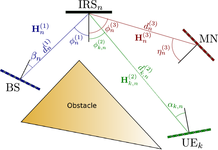
Figure 1: Communication model: a base station (BS) is transmitting toward the $k$-th UE, thanks to the help of the $n$-th IRS. The LoS link between BS and UE is blocked by an obstacle. The $k$-th UE is the victim of the malicious node (MN), which intercepts the signals reflected by the IRSs.

2 Related Work

The main research area our work is related to is physical-layer security for IRS-assisted wireless networks.

As discussed in [15], IRSs can be efficiently used to improve the security and privacy of wireless communications, as they can make the channel better for legitimate users, and worse for malicious ones. As an example, the authors of [16] targeted the case of aligned eavesdroppers, lying between the transmitter and the legitimate receiver: in this case, the authors envisioned avoiding direct transmissions, and using IRSs to maximize the secrecy rate.

Jamming is an effective, even if harsh, method to improve privacy by making the eavesdropper’s channel worse: as an example, [17] envisioned using IRSs to both serve legitimate users and jam the malicious one, maximizing the secrecy rate subject to power constraints. In MIMO scenarios, passive eavesdroppers can be blinded through standard beamforming techniques, thanks to the so-called secrecy-for-free property of MIMO systems with large antenna arrays. Several recent works, including [9], aimed at achieving the same security level against active attackers, by leveraging filtering techniques and the fact that legitimate and malicious nodes are statistically distinguishable from each other. In a similar scenario, [8] presented an alternating optimization that jointly optimizes both transmitter and IRS parameters in order to maximize the secrecy rate. The authors of [10] addressed a vehicular scenario, finding that IRSs are more effective than leveraging vehicular relays to attain physical-layer security.

Many works focussed on the problem of configuring the IRSs available in a given scenario to optimize one or more target metrics, e.g., performance, secrecy rate, or cost. Examples include [11], where an iterative algorithm is used to optimize the sum-rate. In a similar setting and with the same objective, [12] resorted to particle-swarm optimization, owing to the problem complexity and to the need for quick convergence; for similar reasons, the authors of [14] leveraged deep reinforcement learning. An unusual twist is represented by [13], which focused on visible-light communication and optimizes the configuration of IRSs (i.e., mirrors) to optimize the sum-rate, through a Kuhn-Munkres algorithm.

All the works we have discussed share two very important features, to wit:

• they seek to find one high-quality IRS configuration, and

• they build such a configuration from the ground up, i.e., optimizing the phase-shifting vectors of the individual IRS elements.

We depart from such features by (i) selecting a set of multiple configurations among which to cycle, and (ii) confine ourselves to configurations where each IRS points to a user, on the grounds that such configurations are very likely to be the most useful, and restricting our attention to them significantly decreases the complexity.

3 Communication Model

We consider a wireless network operating in the THz bands, composed of:

• A base station (BS) equipped with a uniform linear array (ULA) of antennas composed of $M_{\rm BS}$ isotropic elements and transmitting $K$ data streams, one for each legitimate user;

• $K$ legitimate users (UEs), each equipped with an ULA composed of $M_{\rm UE}$ isotropic antenna elements;

• $N$ IRSs ($N\geq K$) composed of arrays of elements (or meta-atoms) arranged in a square grid. The IRSs contribute to the BS-UEs communication by appropriately forwarding the BS signal toward the users. Notice that, given $K$ legitimate UEs, at any time instant only $K$ IRSs are used.

• A passive eavesdropper (or malicious node, MN), whose ULA is composed of $M_{\rm MN}$ isotropic antenna elements. The goal of the MN is to eavesdrop the communication from the BS towards one of the $K$ legitimate UEs, by intercepting the signals reflected by the IRSs. To do so, the MN exploits the directivity provided by its ULA by pointing it towards the IRS serving the UE that the MN wants to eavesdrop.

We assume ULA made of isotropic elements whose gain is 0 dBi. In practice, each element of the ULA is driven by a phase shifter; thus, by adjusting the phase relationship between the antenna elements, the ULA radiation pattern can be manipulated to generate and steer the beam in a specific direction, or change its shape. Interestingly, in next-generation telecommunication and radar systems, it is envisioned that phased arrays are replaced with transmitarrays, i.e., high-gain antenna systems manufactured with multi-layer printed circuit technology (usually on low-loss substrates as, e.g., quartz or silicon) designed for applications in the 10–300 GHz frequency range.

In the following, boldface uppercase and lowercase letters denote matrices and column vectors, respectively, while uppercase calligraphic letters are used for sets. ${\bf I}_{k}$ is the $k\times k$ identity matrix. For any matrix ${\bf A}$, its transpose and conjugate transpose are denoted by ${\bf A}^{\mathsf{T}}$ and ${\bf A}^{\mathsf{H}}$, respectively, while $[{\bf A}]_{i,j}$ is its $(i,j)$-th element. Finally, the symbol $\otimes$ denotes the Kronecker product.

Below, we characterize the main elements of the system, namely, the channel and the IRSs (Sec. 3.1), as well as the other network nodes and their behavior (Sec. 3.2). To this end, we initially assume that the position of the eavesdropper (hence, the channel conditions it experiences) is known, so that we can characterize the system performance in a clear manner. Importantly, as also remarked later, this is not an assumption required by our algorithm or solution concept and will be dropped in the following sections.

3.1 Channel model and IRS characterization

We assume that no line-of-sight (LoS) path exists between the BS and the UEs. However, communication is made possible by the ability of the IRSs to reflect the BS signal towards the users [18]. Instead, the BS–IRS and IRS-UE links are LoS as well as the IRS–MN link, as depicted in Fig. 1. Also, the BS, all IRSs and user nodes, including the MN, are assumed to have the same height above ground. This assumption allows simplifying the discussion and the notation while capturing the key aspects of the system. In the following, we detail the channel model and the IRS configuration.

Communication channel. While in many works dealing with communications on GHz bands, the channel connecting two multi-antenna devices is often modeled according to Rayleigh or Rice distributions, in the THz bands the channel statistic has not yet been completely characterized. Moreover, at such high frequencies, the signal suffers from strong free-space attenuation, and it is blocked even by small solid obstacles. In practice, the receiver needs to be in LoS with the transmitter to be able to communicate. Also, recent studies [19] have highlighted that already at sub-THz frequencies all scattered and diffraction effects can be neglected. Multipath, if present, is due to reflection on very large objects which, however, entails severe reflection losses. As an example, a plasterboard wall has a reflection coefficient of about -10 dB for most of the incident angles [20]. In practice, the number of paths is typically very small and even reduces to one, i.e., the LoS component, when large high-gain antennas are used [21]. This situation occurs when the transmitter and the receiver adopt massive beamforming techniques that generate beams with very small beamwidth in order to concentrate the signal energy along a specific direction and compensate for high path losses. In such conditions, non-LoS (NLos) paths are very unlikely to show.

Beamforming clearly improves the security of communication since a malicious user must be located within the beam cone to be able to eavesdrop the signal. In addition, spatial diversity and beam configuration switching can make (on average) the channel between the BS and the eavesdropper and the one between the legitimate user and the BS differ, thus further improving security.

In this work, we denote with $M_{\rm tx}$ and $M_{\rm rx}$ the number of antennas at the transmitter and at the receiver, respectively, the $M_{\rm rx}\times M_{\rm tx}$ channel matrix between any two devices can be modeled as:

$${\bf H}^{\rm LOS}=ag{\bf p}{\bf q}^{\mathsf{H}}\,.$$ (1)

In (1), scalar $a$ takes into account large-scale fading effects due to, e.g., obstacles temporarily crossing the LoS path between transmitter and receiver, while coefficient $g$ accounts for the attenuation and phase rotation due to propagation. More specifically, let $d$ be the distance between the transmitting and the receiving device and $\lambda$ the signal wavelength. For the BS-IRS (IRS-UE) link, we denote with $G$ be the array gain of the transmitter (receiver) and with $S$ the effective area of the receiver (transmitter). Then the expression for $g$ is given by:

$$g=\sqrt{\frac{GS}{4\pi d^{2}}}{\rm e}^{{\rm j}\frac{2\pi}{\lambda}d}\,.$$ (2)

Finally, vector ${\bf p}$ of size $M_{\rm rx}$ and vector ${\bf q}$ of size $M_{\rm tx}$ are norm-1 and represent the spatial signatures of, respectively, the receive and the transmit antenna array. The spatial signature of an ULA composed of $M_{\rm z}$ ($z\in\{{\rm BS},{\rm UE},{\rm MN}\}$) isotropic elements, spaced by $\lambda/2$ and observed from an angle $\beta$ (measured with respect to a direction orthogonal to the ULA), is given by the $M_{z}$-size vector ${\bf s}(\beta,M_{z})$, whose $m$-th element is given by:

$$[{\bf s}(\beta,M_{z})]_{m}=\frac{1}{\sqrt{M_{z}}}{\rm e}^{-{\rm j}\frac{\pi}{2}(M_{z}-1)\sin\beta}{\rm e}^{-{\rm j}\pi(m-1)\sin\beta}\,.$$ (3)

This relation applies to devices equipped with ULAs such as the BS, the UEs, and the MN. However, it can also be applied to IRSs with elements spaced by $\lambda/2$, since their planar configuration can be viewed as a superposition of several ULAs.

IRS characterization. IRSs are made of meta-atoms (modeled as elementary spherical scatterers) whose scattered electromagnetic field holds in the far-field regime [22, 23]. We assume that the meta-atoms can reflect the impinging signal without significant losses and apply to it a (controlled) continuous phase shift, which is independent of the frequency. Such IRS model, although ideal, has been widely used [twc22] and holds with a fairly good approximation if the transmitted signal lies in the IRS operational bandwidth which, in the most common designs, amounts to about 10-15% of the central frequency.

The $n$-th IRS, $n=1,\ldots,N$, is composed of $L_{n}^{2}$ meta-atoms arranged in an $L_{n}\times L_{n}$ square grid and spaced by $\lambda/2$. Thus, the area of the $n$-th IRS is given by $A_{n}=L_{n}^{2}\lambda^{2}/4$. The meta-atom at position $(\ell,\ell^{\prime})$ in the $n$-th IRS applies a phase-shift $\theta_{n,\ell,\ell^{\prime}}$, to the signal impinging on it. In many works that assume rich scattering communication channels such phase-shifts are independently optimized in order to maximize some performance figures. However, under the channel model in (1), phase-shifts are related to each other according to the linear equation [24, 25]:

$$\theta_{n,\ell,\ell^{\prime}}=\pi q_{n}\left(\ell-1-\frac{L_{n}-1}{2}\right)+\psi_{n}$$ (4)

where $q_{n}$ and $\psi_{n}$ control, respectively, the direction and the phase of the reflected signal. For simplicity, we can arrange the phase shifts $\theta_{n,\ell,\ell^{\prime}}$ in the diagonal matrix

$$\bar{\boldsymbol{\Theta}}_{n}={\bf I}_{L_{n}}\otimes\boldsymbol{\Theta}_{n}$$

where $\boldsymbol{\Theta}_{n}=\mathrm{diag}({\rm e}^{{\rm j}\theta_{n,1,\ell^{\prime}}},\ldots,{\rm e}^{{\rm j}\theta_{n,L_{n},\ell^{\prime}}})$. Also, we recall that $\otimes$ denotes the Kronecker product and ${\bf I}_{L_{n}}$ is the identity matrix of size $L_{n}$. To clarify how IRSs are configured, consider the example depicted in Fig. 1 where $\phi^{(1)}_{n}$ is the angle of arrival (AoA) of the BS signal on the $n$-th IRS and $\phi^{(2)}_{n,k}$ is the direction of the $k$-th UE as observed from the $n$-th IRS. Then, to let the $n$-th IRS reflect the BS signal towards the $k$-th UE, we set $q_{n}=q_{n,k}$ in (4) where [18]:

$$q_{n,k}=\sin\phi^{(1)}_{n}-\sin\phi^{(2)}_{n,k}\,.$$ (5)

In a scenario with many IRSs and many UEs, where an IRS serves at most a single UE, we can define a map, $c$, between the set of UEs and the set of IRSs, defined as

$$c:\{1,\ldots,K\}\to\{1,\ldots,N\}.$$

This map, in the following referred to as configuration, specifies which UE is served by which IRS. We also denote as $\nu_{c}(k)\in{\cal N}$ the UE served by the $k$-th IRS under configuration $c$. It follows that, if $\nu_{c}(k)=n$, we mean that UE $k$ is served by IRS $n$; in this case, the parameter $q_{n}$ of the $n$-th IRS has to take the value in (5). With $N$ IRSs and $K$ UEs, the number of possible configurations is $C=N!/(N-K)!$ and the corresponding set is denoted by ${\cal C}$. Under configuration $c\in{\cal C}$,

• IRS $\nu_{c}(k)$ forwards the BS signal towards the $k$-th UE and, by symmetry, we assume that the $k$-th UE points its beam towards the $\nu_{c}(k)$-th IRS;

• we denote by $\bar{\boldsymbol{\Theta}}_{n,c}$ the matrix of the phase-shifts at the $n$-th IRS.

An example of possible configurations for a network composed of $N=3$ IRSs and $K=3$ UEs is depicted in Fig. 2.

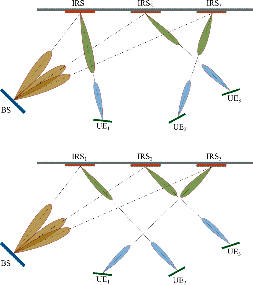
Figure 2: Two possible configurations for a network with $N=K=3$. The top configuration corresponds to the map $\nu_{a}(1)=1$, $\nu_{a}(2)=3$, and $\nu_{a}(3)=2$, while the bottom configuration corresponds to the map $\nu_{b}(1)=3$, $\nu_{b}(2)=1$, and $\nu_{b}(3)=2$.

3.2 Behavior of BS, UEs, and MN

Base station. The BS transmits a signal with bandwidth $B$ and wavelength $\lambda$. Such signal contains $K$ data streams, one for each UE. Let $x_{k}$ be the zero-mean, unit-variance Gaussian complex i.i.d. random symbol generated for the $k$-th stream at a given time. Also, let $\boldsymbol{\gamma}_{k}$ be the beamforming vector of size $M_{\rm BS}$, employed for transmitting $x_{k}$. Then, the signal transmitted by the BS is given by the size-$M_{\rm BS}$ vector

$${\bf t}=\boldsymbol{\Gamma}{\bf x}$$ (6)

where $\boldsymbol{\Gamma}=[\boldsymbol{\gamma}_{1},\ldots,\boldsymbol{\gamma}_{K}]$ is the $M_{\rm BS}\times K$ precoding matrix and ${\bf x}=[x_{1},\ldots,x_{K}]^{\mathsf{T}}$. We assume that the total transmit power is limited by $P_{t}$, i.e., $\mathbb{E}[|{\bf t}|^{2}]=\|\boldsymbol{\Gamma}\|_{\rm F}^{2}\leq P_{t}$, with $\|\cdot\|_{\rm F}$ denoting the Frobenius norm.

Legitimate receivers (UEs). The signal received by the $k$-th UE under the $c$-th configuration is given by [18]

$$r_{k,c} = \underbrace{{\bf f}_{k,c}^{\mathsf{H}}\sum_{n=1}^{N}{\bf H}^{(2)}_{k,n}\bar{\boldsymbol{\Theta}}_{n,c}{\bf H}^{(1)}_{n}}_{\widetilde{{\bf h}}_{n,c}^{\mathsf{H}}}{\bf t}+n_{k}$$ (7)

where

• $n_{k}\sim{\cal N}_{\mathbb{C}}(0,N_{0}B)$ is additive Gaussian complex noise with zero-mean and variance $N_{0}B$, and $N_{0}$ is its power spectral density;

• the size-$M_{\rm UE}$ vector ${\bf f}_{k,c}$ represents the beamforming at the $k$-th UE under the $c$-th configuration. In particular, we assume that the UE’s ULA is only capable of analog beamforming; thus, ${\bf f}_{k,c}={\bf s}(\alpha_{k,n},M_{\rm UE})$ where $n=\nu_{c}(k)$, i.e., the radiation pattern of the $k$-th UE ULA points to the $\nu_{c}(k)$-th IRS;

• ${\bf H}^{(1)}_{n}$ is the $L_{n}^{2}\times M_{\rm BS}$ channel matrix connecting the BS to the $n$-th IRS; according to the channel model in (1), it is given by ${\bf H}^{(1)}_{n}=a_{n}^{(1)}g_{n}^{(1)}{\bf p}_{n}^{(1)}{{\bf q}_{n}^{(1)}}^{\mathsf{H}}$ where ${\bf q}_{n}^{(1)}\mathord{=}{\bf s}(\beta_{n},M_{\rm BS})$, ${\bf p}_{n}^{(1)}\mathord{=}\frac{1}{\sqrt{L_{n}}}{\bf 1}_{L_{n}}\otimes\bar{{\bf p}}_{n}^{(1)}$ and $\bar{{\bf p}}_{n}^{(1)}={\bf s}(\phi^{(1)}_{n},L_{n})$. Moreover, $g^{(1)}_{n}\mathord{=}\frac{\sqrt{M_{\rm BS}A_{n}}}{\sqrt{4\pi}d^{(1)}_{n}}{\rm e}^{{\rm j}\frac{2\pi}{\lambda}d^{(1)}_{n}}$ and $d^{(1)}_{n}$ is the distance between the BS and the $n$-th IRS;

• ${\bf H}^{(2)}_{k,n}\mathord{=}a^{(2)}_{k,n}g^{(2)}_{k,n}{\bf p}_{n,k}^{(2)}{{\bf q}_{n,k}^{(2)}}^{\mathsf{H}}$ is the $M_{\rm UE}\times L_{n}^{2}$ channel matrix connecting the $n$-th IRS to the $k$-th UE where, according to (1), we have ${\bf p}_{k,n}={\bf s}(\alpha_{k,n},M_{\rm UE})$ and ${\bf q}_{n,k}^{(2)}=\frac{1}{\sqrt{L_{n}}}{\bf 1}_{L_{n}}\otimes\bar{{\bf q}}_{k,n}^{(2)}$. Moreover, $\bar{{\bf q}}_{k,n}^{(2)}\mathord{=}{\bf s}(\phi_{k,n}^{(2)},L_{n})$ and $g^{(2)}_{k,n}=\frac{\sqrt{M_{\rm UE}A_{n}}}{\sqrt{4\pi}d^{(2)}_{n,k}}{\rm e}^{{\rm j}\frac{2\pi}{\lambda}d^{(2)}_{n,k}}$. Finally, $d^{(2)}_{n,k}$ is the distance between the $n$-th IRS and $k$-th UE.

Notice that, by assuming that all network nodes have the same height over the ground, the $n$-th IRS can be viewed as a superposition of $L_{n}$ identical ULAs. Thus, its spatial signature can be written in a compact form by using the Kronecker product, as indicated above. Also, the angles $\beta_{n}$, $\phi_{n}^{(1)}$, $\phi_{k,n}^{(2)}$, and $\alpha_{k,n}$ are specified in Fig. 1 and are measured with respect to the normal to the corresponding ULA or IRS.

By collecting in vector ${\bf r}_{c}=[r_{1,c},\ldots,r_{K,c}]^{\mathsf{T}}$ the signals received by the $K$ UEs and by recalling (6), we can write:

$${\bf r}_{c}=\widetilde{{\bf H}}_{c}^{\mathsf{H}}{\bf t}+{\bf n}=\widetilde{{\bf H}}_{c}^{\mathsf{H}}\boldsymbol{\Gamma}{\bf x}+{\bf n}$$ (8)

where $\widetilde{{\bf H}}_{c}=[\widetilde{{\bf h}}_{1,c},\ldots,\widetilde{{\bf h}}_{K,c}]$ and ${\bf n}=[n_{1},\ldots,n_{K}]^{\mathsf{T}}$.

Malicious node. By eavesdropping the communication, the MN acts as an additional receiver. When configuration $c$ is applied and the MN’s ULA points to the $n$-th IRS, the received signal can be written similarly to (7), as

$$o_{n,c} = \underbrace{{\bf b}_{n}^{\mathsf{H}}\sum_{m=1}^{N}{\bf H}_{m}^{(3)}\bar{\boldsymbol{\Theta}}_{m,c}{\bf H}_{m}^{(1)}}_{\widetilde{{\bf b}}_{n,c}^{\mathsf{H}}}{\bf t}+\zeta$$ (9)

where ${\bf H}_{m}^{(3)}=a_{m}^{(3)}c_{m}^{(3)}{\bf p}_{m}^{(3)}{{\bf q}_{m}^{(3)}}^{\mathsf{H}}$ is the $L_{n}^{2}\times M_{\rm MN}$ channel matrix connecting the $n$-th IRS to the MN, ${\bf p}_{m}^{(3)}={\bf s}(\eta_{m}^{(3)},M_{\rm MN})$, ${\bf q}_{m}^{(3)}=\frac{1}{\sqrt{L_{m}}}{\bf 1}_{L_{m}}\otimes\bar{{\bf q}}_{m}^{(3)}$, $\bar{{\bf q}}_{m}^{(3)}={\bf s}(\phi^{(3)}_{m},L_{m})$ (see Fig. 1). Also, $g_{m}^{(3)}=\frac{\sqrt{M_{\rm MN}A_{m}}}{\sqrt{4\pi}d^{(3)}_{m}}{\rm e}^{{\rm j}\frac{2\pi}{\lambda}d^{(3)}_{m}}$ where $d^{(3)}_{m}$ is the distance between the MN and the $m$-th IRS. Finally, $\zeta\sim{\cal N}_{\mathbb{C}}(0,N_{0}B)$ represents the additive noise at the receiver and ${\bf b}_{n}={\bf s}(\eta_{n}^{(3)},M_{\rm MN})$ is the norm-1 beamforming vector.

4 Network Management Mechanism

Under our network management mechanism, the BS and the legitimate nodes switch, periodically and in a synchronized manner, between different configurations, i.e., IRS-to-UE assignment. So doing, they can counteract the eavesdropper’s efforts at guessing the current configuration. At the same time, the BS must be careful not to use configurations with poor performance, i.e., yielding a low data rate. Let us denote with $R(k,c)$ the rate experienced by user $k$ under configuration $c\in{\cal C}$, and with $\text{SR}(n,k,c)$ the secrecy rate obtained under configuration $c$ when the victim is user $k$ and the eavesdropper is listening to IRS $n$. Furthermore, let $k^{\star}$ identify the eavesdropper’s victim.

In the following, we first define the performance metrics of interest, namely, the data rate and the secrecy rate of legitimate users (Sec. 4.1); then, we introduce the communication scheme that is adopted by the BS, the legitimate users, and the MN (Sec. 4.2).

4.1 Performance metrics

The SINR achieved at each UE depends on the precoding strategy employed at the BS, i.e., on the choice of the precoder $\boldsymbol{\Gamma}$. For example, the zero-forcing (ZF) precoder permits to remove the inter-user interference while providing good (although not optimal) performance. Under the $c$-th configuration, $\nu_{c}$, the ZF precoder is obtained by solving for $\boldsymbol{\Gamma}_{c}$ the equation $\widetilde{{\bf H}}_{c}^{\mathsf{H}}\boldsymbol{\Gamma}_{c}=\mu\boldsymbol{\Pi}$ where $\boldsymbol{\Pi}=\mathrm{diag}(\pi_{1},\ldots,\pi_{K})$ is an arbitrary positive diagonal matrix and the scalar $\mu$ should be set so as to satisfy the power constraint $\|\boldsymbol{\Gamma}_{c}\|_{\rm F}^{2}\leq P_{t}$. The diagonal elements of $\boldsymbol{\Pi}$ specify how the transmit power is shared among users; as an example, if $\boldsymbol{\Pi}$ is proportional to the identity matrix, the same fraction of signal power is assigned to each UE. The expression of the ZF precoder $\boldsymbol{\Gamma}_{c}$ is then given by:

$$\boldsymbol{\Gamma}_{c}\triangleq\frac{\sqrt{P_{t}}\widetilde{{\bf H}}_{c}^{+}\boldsymbol{\Pi}^{\frac{1}{2}}}{\|\widetilde{{\bf H}}_{c}^{+}\boldsymbol{\Pi}^{\frac{1}{2}}\|_{\rm F}}$$ (10)

where $\widetilde{{\bf H}}_{c}^{+}=\widetilde{{\bf H}}_{c}^{\mathsf{H}}(\widetilde{{\bf H}}_{c}\widetilde{{\bf H}}_{c}^{\mathsf{H}})^{-1}$ is the Moore-Penrose pseudo-inverse of $\widetilde{{\bf H}}_{c}$.

The SINR at the $k$-th UE is then given by:

$${\rm SINR}^{{\rm UE}}_{k,c}=\frac{P_{t}}{N_{0}B\|\widetilde{{\bf H}}_{c}^{+}\boldsymbol{\Pi}^{\frac{1}{2}}\|^{2}_{\rm F}}\,.$$ (11)

Similarly, we can write the SINR at the MN when the latter points its ULA to the $n$-th IRS while eavesdropping the data stream intended for UE $k$, as

$${\rm SINR}^{{\rm MN}}_{n,k,c}=\frac{\pi_{k}|\widetilde{{\bf b}}_{n,c}^{\mathsf{H}}\boldsymbol{\gamma}_{k,c}|^{2}}{\sum_{h\neq k}\pi_{h}|\widetilde{{\bf b}}_{n,c}^{\mathsf{H}}\boldsymbol{\gamma}_{h,c}|^{2}+N_{0}B}$$ (12)

where $\boldsymbol{\gamma}_{k,c}$ is the $k$-th column of $\boldsymbol{\Gamma}_{c}$ whose expression is given in (10), and $\widetilde{{\bf b}}_{n,c}^{\mathsf{H}}$ is defined in (9).

The data rate for UE $k$ under the $c$-th configuration can be computed as

$$R(k,c)=B\log_{2}\left(1+{\rm SINR}^{{\rm UE}}_{k,c}\right)\,.$$ (13)

Finally, the secrecy rate (SR) obtained when the MN eavesdrops the data stream intended for UE $k$, by pointing its antenna to the IRS $n$, under configuration $c$, is given by:

$${\rm SR}(n,k,c)=\max\big{\{}0,R(k,c)\mathord{-}B\log_{2}(1\mathord{+}{\rm SINR}^{{\rm MN}}_{n,k,c})\big{\}}\,.$$ (14)

The $\max$ operator in (14) is required since, under certain circumstances, ${\rm SINR}^{{\rm MN}}_{n,k,c}$ might be larger than ${\rm SINR}^{{\rm UE}}_{k,c}$.

4.2 Communication scheme

Let us normalize time quantities to the time it takes to receivers (legitimate or not) to switch from one configuration to another, and call such time interval time unit.

Given ${\cal C}$, the BS chooses a set $\bar{{\cal C}}\subseteq{\cal C}$ of configurations to activate, as well as a criterion that legitimate users shall follow to determine the next configuration to move to. In other words, legitimate nodes will always know the next configuration to use while the eavesdropper cannot. A simple way to achieve this is to use hash chains [26]: the first element of the chain (i.e., the first configuration to activate) is a secret shared among all legitimate nodes. Then, subsequent elements of the chain – hence, subsequent configurations – are achieved by hashing the current element, in a way that is easy for honest nodes to compute, but impossible for an outsider to guess. We further assume that all chosen configurations are used with equal probability, and that they are notified to legitimate users in a secure manner, while the eavesdropper has no way of knowing the next configuration in advance. As noted earlier, hash chains allow us to attain both goals.

The decision about whether or not to use configuration $c$ is expressed through binary variables $y(c)$, which take 1 if $c$ is adopted and 0 otherwise. Given the value of the decision variables $y(c)$, we can write the probability $\omega(k,n)$ that user $k$ is served through IRS $n$ under any of the chosen configurations $c\in\bar{{\cal C}}$, as

$$\omega(k,n)=\frac{\sum_{c\in\bar{{\cal C}}}\mathds{1}_{[\nu_{c}(k)=n]}}{\left|\bar{{\cal C}}\right|}\,.$$ (15)

As for the eavesdropper, we consider the most unfavorable scenario for the legitimate users and assume that the MN has already estimated the probability with which its victim is served by each IRS, and that it can leverage such information by pointing its own beam towards each IRS according to those probabilities.

Given $\bar{{\cal C}}$, the BS sets the number of time units $\tau\geq 1$ for which the legitimate users should stay with any configuration $c\in\bar{{\cal C}}$. Then, considering the fact that one time unit is the time needed to switching configuration and the communication is paused during such switching time (i.e., every $\tau+1$), it follows that the average rate for each legitimate user $k$ can be written as:

$$R_{\text{avg}}(k)=\frac{\tau}{\tau+1}\frac{\sum_{c\in\bar{{\cal C}}}R(k,c)}{\left|\bar{{\cal C}}\right|}\,.$$ (16)

Moving to the eavesdropper, its objective is to have the smallest possible secrecy rate (SR) for its victim $k^{\star}$. There are two strategies it can follow towards this end:

• static: to always point towards the IRS that is most frequently used to serve the victim $k^{\star}$, i.e.,
  $n^{\star}=\arg\max_{n}\omega(k^{\star},n)$, or

• dynamic: to spend $\delta$ time units to try all IRSs, identify the one serving the victim $k^{\star}$, and then point towards it.

In the first case, the resulting SR is given by:

$$\text{SR}_{\text{avg}}^{\text{static}}(k^{\star})=\frac{1}{\left|\bar{{\cal C}}\right|}\sum_{c\in\bar{{\cal C}}}\text{SR}(n^{\star},k^{\star},c)\,,$$ (17)

while in the latter case, the SR is as follows:

$$\text{SR}_{\text{avg}}^{\text{dynamic}}(k^{\star})=\begin{cases}\sum_{c\in\bar{{\cal C}}}\left[\frac{\tau\mathord{-}\delta}{\tau}\min_{n}\text{SR}(n,k^{\star},c)\mathord{+}\frac{\delta R(k^{\star},c)}{\tau}\right]\\ \quad\qquad\qquad\qquad\,\text{if~{}$\delta\leq\tau$}\\ \frac{1}{\left|\bar{{\cal C}}\right|}R(k^{\star},c)\qquad\,\,\,\text{else}.\end{cases}$$ (18)

The quantity within square brackets in (18) comes from the fact that, for each configuration (i.e., each $\tau$ time units), the eavesdropper spends $\delta$ units trying all IRSs (during which the SR will be $R(k^{\star},c)$, i.e., complete secrecy), and $\tau-\delta$ units experiencing the minimum secrecy rate across all IRSs. In both cases, SR values are subordinate to the fact that the BS is transmitting – clearly, if there is no transmission, there can be no secrecy rate. Also, notice how we must write SR values as dependent upon the eavesdropping victim $k^{\star}$; indeed, the eavesdropper knows who its victim is, while legitimate users do not.

The eavesdropper will choose the strategy that best suits it, i.e., results in the lowest secrecy rate. It follows that the resulting secrecy rate is:

$$\text{SR}_{\text{avg}}(k^{\star})=\min\left\{\text{SR}_{\text{avg}}^{\text{static}}(k^{\star}),\text{SR}_{\text{avg}}^{\text{dyn}}(k^{\star})\right\}\,.$$

5 Problem Formulation and Solution Strategy

In this section, we first formulate the choice of set $\bar{{\cal C}}\subseteq{\cal C}$ of configurations to enable as an optimization problem. Then, in light of the problem complexity, we propose an efficient heuristic called ParallelSlide, and we show that the proposed algorithm obtains solutions provably close to the optimum in a remarkably short time.

5.1 Problem formulation

The goal of the network system is to maximize the average secrecy rate over time, so long as all legitimate users get at least an average rate $R_{\min}$, i.e.,

$$\max_{\bar{{\cal C}},\tau}\min_{k}\text{SR}_{\text{avg}}(k)$$ (19)

$$\text{s.t.}\quad R_{\text{avg}}(k)\geq R_{\min},\quad\forall k\,.$$ (20)

Notice how objective (19) must be stated in a max-min form: since the BS does not know who the eavesdropping victim is, it aims at maximizing the secrecy rate in the worst-case scenario, in which the node with the lowest SR is indeed the victim.

Furthermore, we remark that, in some cases, it may be necessary to use the same configuration $c\in{\cal C}$ multiple times before repeating the cycle, i.e., to replicate a selected configuration. Our system model and notation do not directly support this, as the decisions about configuration activation are binary (or, equivalently, a configuration cannot appear in set $\bar{{\cal C}}$ more than once). However, it is possible to obtain the same effect as repeating a configuration, by including several replicas thereof in $\bar{{\cal C}}$: in this case, the data and secrecy rates of each replica of the configuration are evaluated separately, hence, the same configuration can be used multiple times if appropriate.

Next, to streamline the notation, let us indicate with $\hat{R}(c)=\min_{k}R(k,c)$ the worst-case rate experienced by a legitimate user under configuration $c\in{\cal C}$, and with $\hat{S}(c)=\min_{n}SR(n,k^{\star},c)$ the minimum secrecy rate experienced by the victim $k^{\star}$ under such a configuration. Importantly, secrecy rate values are averaged over (in principle) all possible positions of the eavesdropper, hence, computing such information requires no knowledge of the eavesdropper’s position or channel quality. Then, let us assume that the attacker follows the dynamic strategy, which has been proven [27] to be the most effective except for very swift configuration changes. By recalling that each configuration $c\in\bar{{\cal C}}$ is held for the same time duration, hence the temporal and the numerical average coincide, we can rewrite (19) as:

$$\max_{\{y(c)\}_{c}} \frac{\delta}{\tau+1}\frac{1}{\sum_{c\in{\cal C}}y(c)}\sum_{c\in{\cal C}}y(c)\hat{R}(c)+$$ (21)

$$+\frac{\tau-\delta}{\tau+1}\frac{1}{\sum_{c\in{\cal C}}y(c)}\sum_{c\in{\cal C}}y(c)\hat{S}(c)$$

$$\mathrm{s.t.} \frac{\tau}{\tau+1}\frac{1}{\sum_{c\in{\cal C}}y(c)}\sum_{c\in{\cal C}}y(c)\hat{R}(c){\geq}R_{\min}\,.$$ (22)

The above expression accounts for the fact that, within each time interval, legitimate users enjoy a secrecy rate equal to the average rate of the selected configurations for a fraction $\frac{\delta}{\tau+1}$ of the time (during which the eavesdropper can hear nothing, hence, the secrecy rate is the same as the UEs’ data rate). For the rest of the time, the secrecy rate is the average of the secrecy rates of the selected configurations. Constraint (22) describes the fact that the system transmits nothing for a fraction $\frac{1}{\tau+1}$ of the time, and legitimate users enjoy the average of the rates of the selected configurations for the rest of the time.

At last, notice that the problem above is combinatorial and nonlinear; hence, it is critical to envision a low-complexity heuristics that can cope with non-trivial instances of the problem while yielding effective solutions.

5.2 Solution strategy: The ParallelSlide algorithm

The NP-hardness of optimizing objective (21) subject to constraint (22) means that making optimal decisions takes a prohibitively long time – possibly, hours or days – even for modestly-sized problem instances. We therefore opt for a heuristic approach, seeking to make high-quality – namely, near-optimal decisions – with small computational complexity, hence, in a short time.

Our high-level goal is to leverage the results of [28], providing very good competitive ratio properties for a simple greedy algorithm, as long as (i) the objective is submodular nondecreasing, and (ii) the constraint is knapsack-like, i.e., additive. We will proceed as follows:

1. Discussing the submodularity of the objective in (21) and of the constraint in (22), showing that they are not submodular in general;

2. Observing that, if the number $|\bar{{\cal C}}|$ of configurations to eventually select were known, then (21) and (22) would be submodular;

3. Exploiting the latter to propose an efficient algorithm solving the original problem.

Submodularity. Recall that a generic set function $f(X)$ is submodular if, for any set ${\cal A}$ and ${\cal B}$ and element $x$, the following holds:

$$f({\cal A}\cup{\cal B}\cup\{x\})-f({\cal A}\cup{\cal B})\leq f({\cal A}\cup\{x\})-f({\cal A}).$$ (23)

Intuitively, adding $x$ to a larger set ${\cal A}\cup{\cal B}$ brings a lower benefit than adding it to a smaller set ${\cal A}$; such an effect is often referred to as “diminishing returns”.

Owing to its simplicity, let us focus on constraint (22) and derive a restrictive, necessary (and sufficient) condition for its submodularity.

Property 1

Constraint (22) is submodular only if configurations are selected from the worst-performing to the best-performing one.

Proof 1

We start from the submodular definition in (23), where in our case ${\cal A}\subseteq{\cal C}$ and ${\cal B}\subseteq{\cal C}$ are sets of configurations. Let $A$ and $B$ denote their cardinality, and $a$ and $b$ define their corresponding average data rate. Furthermore, let $\rho=\hat{R}(c^{\prime})$ be the rate of the new configuration $c^{\prime}\in{\cal C}$. Keeping in mind that the $\frac{\tau}{\tau+1}$ terms simplify away, (23) becomes:

$$\frac{Aa{+}Bb{+}\rho}{A{+}B{+}1}{-}\frac{Aa{+}Bb}{A{+}B}\leq\frac{Aa{+}\rho}{A{+}1}{-}\frac{Aa}{A},$$ (24)

which simplifies to

$$a(2A+B+1)\leq(A+1)b+\rho(A+B),$$ (25)

Notice that (25) holds if $\rho\geq b\geq a$, as per the hypothesis.

The condition derived in Property 1 is very restrictive; indeed, there is no good reason why the worst-performing configurations should be chosen first. Also notice that the non-submodularity of objective (21) can be proven through the very same argument.

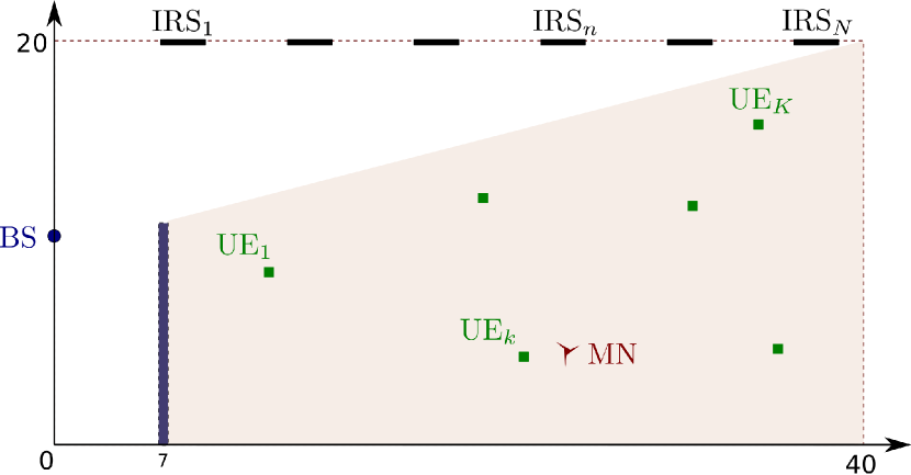
Figure 3: Base scenario.

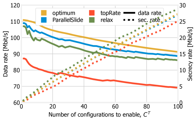
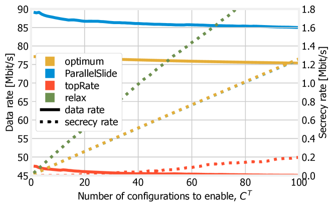
Figure 4: Data rate and secrecy rate achieved as the number $C^{\text{T}}$ of configurations to choose changes, under the base (left) and extended (right) scenarios.

Adding an oracle: the ParallelSlide algorithm. Intuitively, what destroys the submodularity of (21)–(22) is the presence of the average, which in turn comes from the fact that we must choose both how many configurations to select, and which ones. Splitting the two parts of the problem would indeed result in a significantly better-behaved problem. More specifically, we can prove that the following property holds.

Property 2

If the number $|\bar{{\cal C}}|$ of configurations to choose is known, then objective (21) is submodular, and constraint (22) is a knapsack constraint.

Proof 2

Concerning the objective, the proof trivially comes from the observation that, once $|\bar{{\cal C}}|$ is known, (21) reduces to a sum of (i) constant quantities, and (ii) decision variables multiplied by positive coefficients.

As for constraint (22), recall that a knapsack constraint over set ${\cal V}$ is an alternate to a cardinality constraint where each element of the set has a cost and the selected items cannot exceed a total budget [29]. We can re-write (22) as:

$$\sum_{c\in{\cal C}}y(c)\hat{R}(c)\geq\frac{\tau}{\tau+1}R_{\min},$$

hence, it is a knapsack constraint.

Property 2 implies that, once $|\bar{{\cal C}}|$ is known, the problem reduces to optimizing a submodular nondecreasing function subject to a knapsack constraint. Such problems can be solved very efficiently by greedy algorithms [28, 29], picking at each step the configuration with the highest benefit-to-cost ratio. We leverage this principle while designing our algorithm, called ParallelSlide and presented in Alg. 1. The basic idea of ParallelSlide is indeed to (i) try all possible sizes of $\bar{{\cal C}}$, and (ii) for each target size, obtain a solution with that size by applying the benefit-to-cost ratio principle of [28, 29]. We remark that the number of possible sizes of $\bar{{\cal C}}$ cannot exceed the minimum between the number of all possible configurations and the maximum number of configurations that it is possible to select, i.e., $|{\cal C}|$.

Specifically, for each value of the target size $C^{\text{T}}$ (Line 3 in Alg. 1), the algorithm builds a solution by first using all configurations (Line 4), and then removing, at each iteration, the configuration which minimizes the ratio between the data rate it yields and the corresponding secrecy rate, as per Line 6. In Line 6, $\hat{R}$ and $\hat{S}$ indicate, respectively, the rate and secrecy rate obtained after activating configuration $c$, accounting for the fact that a total of $C^{\text{T}}$ configurations will eventually be activated.

Upon reaching size $C^{\text{T}}$, the algorithm checks if set used\_configs results in a feasible solution (Line 8) and, if so, adds it to the set feasible\_solutions (Line 9). After trying out all possible values of $C^{\text{T}}$, the solution resulting in the best performance, i.e., the largest value of objective (21), is selected.

5.3 Algorithm analysis

The ParallelSlide algorithm has two very good properties, namely (i) it has a very low computational complexity, and (ii) it provides results that are provably close to the optimum. Let us begin from the former result.

Property 3

The ParallelSlide algorithm has quadratic worst-case computational complexity, namely, $O(|{\cal C}|^{2})$.

Proof 3

The proof comes by inspection of Alg. 1. The algorithm contains two loops: an outer one (beginning in Line 3 that runs exactly $|{\cal C}|$ times), and an inner one (beginning in Line 5 that runs at most $|{\cal C}|$ times). All other operations, e.g., checking feasibility in Line 8, are elementary and are run fewer than $|{\cal C}|^{2}$ times. Hence, the final worst-case computational complexity is $O(|{\cal C}|^{2})$.

Its quadratic complexity allows ParallelSlide to make swift decisions, and makes it suitable for real-time usage.

Algorithm 1 The ParallelSlide algorithm

1:${\cal C}$

2:$\text{\path{feasible\_solutions}}\leftarrow\emptyset$

3:for all $C^{\text{T}}\in[|{\cal C}|,\dots,1]$ do

4:     $\text{\path{used\_configs}}\leftarrow{\cal C}$

5:     while $|\text{\path{used\_configs}}|>C^{\text{T}}$ do

6:         $\text{\path{to\_del}}\leftarrow\arg\min_{c\in\text{\path{used\_configs}}}\frac{\mathbf{\hat{R}}(c,C^{\text{T}})}{\mathbf{\hat{S}}(c,C^{\text{T}})}$

7:         $\text{\path{used\_configs}}\leftarrow\text{\path{used\_configs}}\setminus\{\text{\path{to\_del}}\}$      

8:     if $\mathbf{is\_feasible}(\text{\path{used\_configs}})$ then

9:         $\text{\path{feasible\_solutions}}\leftarrow$

10:         *$\text{\path{feasible\_solutions}}\cup\{\text{\path{used\_configs}}\}$      return $\arg\max_{\text{\path{s}}\in\text{\path{feasible\_solutions}}}\mathbf{secrecy\_rate}(s)$

Concerning the quality of decisions, we are able to prove that:

• ParallelSlide is remarkably close to the optimum, and

• the distance between ParallelSlide and the optimum does not depend upon the problem size.

More formally, the ratio of the objective value (21) obtained by ParallelSlide to the optimal one is called competitive ratio. In most cases, competitive ratios decrease (i.e., the solutions get worse) as the problem size increases; intuitively, larger problems are harder to solve. This is not the case of ParallelSlide, whose competitive ratio is constant, as per the following property:

Property 4

The ParallelSlide algorithm has a constant competitive ratio of $0.405$.

Proof 4

The proof comes from observing that the inner loop of Alg. 1, i.e., the one starting at Line 3, mimics the MGreedy algorithm presented in [29, Alg. 1]. Our problem has one additional potential source of suboptimality, namely, the choice of the number $C^{\text{T}}$ of configurations to choose; however, the outer loop of Alg. 1 tries out all possible values of $C^{\text{T}}$ (Line 3) and chooses the one resulting in the best performance (Line 10). It follows that no further suboptimality is introduced, and ParallelSlide has the same competitive ratio as [29, Alg. 1], namely, $0.405$.

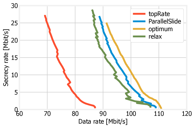
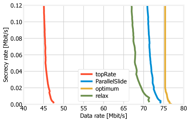
Figure 5: Trade-offs between data rate and secrecy rate attained by different strategies, under the base (left) and extended (right) scenarios.

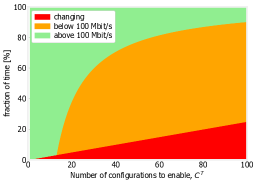
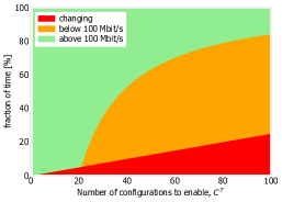
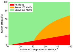
Figure 6: Base scenario: fraction of time spent by nodes enacting higher-data rate configurations (green), enacting lower-data rate configurations (orange), or switching between configurations (red), under the topRate (a), ParallelSlide (b), and optimum (c) strategies.

Finally, we can prove that ParallelSlide does in fact convergence after a finite number of iterations:

Property 5

The ParallelSlide algorithm converges after at most $|{\cal C}|^{2}$ iterations.

Proof 5

The proof comes by the inspection of Alg. 1, which has two nested loops, each of which runs at most $|{\cal C}|$ times.

So far, we have presented and discussed ParallelSlide with reference to a scenario where no LoS path from the BS to any user exists. These are indeed the most challenging scenarios, and those where IRSs are most useful; however, ParallelSlide works unmodified when direct paths do exist. Specifically:

• the set of IRSs is extended with an extra item $\varnothing$, indicating that the direct path is used;

• additional configurations are generated accordingly;

• ParallelSlide is applied to the new set of configurations, with no change.

6 Performance Evaluation

To study the performance of ParallelSlide, we consider a scenario where BS, UEs, IRSs and the MN are located in a room of size 40 m$\times$20 m (see Figure 3 for details). As can be observed, the BS–UEs LoS path is unavailable since it is blocked by an obstacle, which is the most challenging scenario for our decision-making process.

The network operates in the sub-terahertz spectrum, namely, at central frequency $f_{c}\mathord{=}100$ GHz, corresponding to the wavelength $\lambda{=}3$ mm. The BS, whose ULA is composed of $M_{\rm BS}{=}32$ isotropic (0 dBi) antenna elements, is located at coordinates $(0,10)$ m; the BS antenna gain is, thus, $G{=}M_{\rm BS}$. The signal bandwidth is $B{=}1$ GHz, and the transmit power is set to $P_{t}{=}10$ dBm. Such power is equally shared among UEs, i.e., the matrix $\boldsymbol{\Pi}$ in (10) is proportional to the identity matrix.

In our scenario all $N$ IRSs are identical, have square shape, and are made of 128$\times$128 meta-atoms, (i.e., $L_{n}{=}128$, $n{=}1,\ldots,N$) with no gaps between them. We also consider that meta-atoms have square shape with side length $\lambda/2$, so that each IRS has area $A=L^{2}\lambda^{2}/4{=}368.64$ cm². Also, IRSs are placed on the topmost wall and equally spaced.

The UEs are uniformly distributed in the shaded area shown in Figure 3. All UEs are equipped with ULAs, each composed of $M_{\rm UE}{=}8$ isotropic (0 dBi) antenna elements, hence their antenna gain is $G{=}M_{\rm UE}$. The malicious node too is equipped with $M_{\rm MN}=8$ isotropic antenna elements and is randomly located around the eavesdropped UE.

In order to study the performance of ParallelSlide in the most challenging conditions, the position of the malicious node is uniformly distributed in a square of side 1 m around the eavesdropped UE. Finally, at both UEs and MN receivers, the noise power spectral density is set to $N_{0}=-174$ dBm/Hz.

Specifically, we consider the following two simple, yet representative, cases:

• a base scenario, including a total of $K{=}6$ legitimate users and $N{=}6$ IRSs, resulting in a total of $|{\cal C}|=6!{=}720$ possible configurations;

• an extended scenario, where we increase the number of users and IRSs to $N{=}K{=}8$ (hence, the number of possible configurations grows to $8!\mathord{=}40\mathord{,}320$).

We compare ParallelSlide against three alternative solutions, namely:

• A simple topRate approach, selecting the $C^{\text{T}}$ configurations with the highest rate;

• A strategy, labelled relax in plots, and performing a relaxation of the problem to solve as per [30];

• The optimum, found through simulated annealing.

The “relax” strategy follows the strategy of [30], and performs the following main operations:

1. It solves an LP (linear problem) relaxation of the problem in (19), where binary variables $y(c)$ are replaced by real ones $\bar{y}\in[0,1]$;

2. It incrementally activates more configurations, choosing them with a probability proportional to $\bar{y}(c)$;

3. It stops upon reaching the target number of configurations.

For simulated annealing, we use the following parameters:

• number of generations: 50;

• solutions per population 100;

• parents mating: 4;

• mutation probability: 15%;

• crossover type: single point;

• gene space: $\{0,1\}$;

• number of genes: $|{\cal C}|$.

Figure 4 depicts how the number $C^{\text{T}}$ of configurations to choose influences the resulting rate and secrecy rate, under ParallelSlide and its counterparts. As it can be expected, the achievable rate (left-hand side scale) is always substantially higher than the secrecy rate (right-hand side scale). The goal of our performance evaluation is not to directly compare the two metrics; rather, we evaluate how different strategies (corresponding to different colors in the plots) impact both metrics (represented by different line styles in the plots).

A first important observation we can make is that solid and dotted curves in the plots, representing (respectively) data rate and secrecy rate, have different slopes. Specifically, choosing more configurations decreases the data rate, as we are forced to include lower-rate IRS-UE assignments. On the other hand, more configurations result in a better secrecy rate, as it takes longer for the eavesdropper to guess the configuration adopted by the legitimate nodes.

Concerning the relationship between the strategies, we can observe that ParallelSlide consistently and significantly outperforms both the “topRate” and “relax” benchmarks, and almost matches the optimum for all values of $C^{\text{T}}$. This validates the intuition from which ParallelSlide stems, i.e., combining both rate and secrecy rate when making configuration-selection decisions, results in better performance. It is also interesting to remark how ParallelSlide’s performance is very close to the optimum, even more than foreseen by the bound in Property 4.

Figure 6 offers additional insights on the different performance of ParallelSlide and its alternatives, summarizing the trade-offs between data rate and secrecy rate they are able to attain. We can observe that ParallelSlide can achieve higher-quality trade-offs; in other words, for a given value of minimum data rate ($R_{\min}$ in (22)), ParallelSlide can obtain a better secrecy rate, i.e., a higher value of the objective in (19).

In summary, we can conclude that ParallelSlide’s ability to account for both data rate and secrecy rate when making configuration-selection decisions allows it to attain high-quality trade-offs between such two quantities, thus outperforming alternative approaches and closely matching the optimum.

We now focus on the base scenario, and seek to better understand the effect of adding more configurations, i.e., increasing $C^{\text{T}}$. To this end, we plot in Figure 6 the fraction of time spent by nodes:

• enacting higher-data rate configurations, resulting in a rate above 100 Mbit/s (green);

• enacting lower-data rate configurations, with a rate below 100 Mbit/s (orange);

• idle, switching between configurations (red).

We can observe that increasing $C^{\text{T}}$ adversely impacts the rate (as per Figure 4) in two main ways. On the one hand, more time is spent switching between configurations, as switches themselves become more frequent. At the same time, selecting more configurations means, necessarily, selecting slower IRS-UE assignments, further decreasing the resulting average rate. Comparing the plots, we can observe that the performance difference between different strategies only comes from the ability to select better (i.e., higher-data rate) configurations, as the time spent switching between configurations only depends upon $C^{\text{T}}$ and is not impacted by the strategy being used.

Overall, Figure 6 confirms our intuition that $C^{\text{T}}$ should only be as large as needed to attain the required secrecy rate, and further increasing it would needlessly hurt the performance.

7 Conclusions

We have addressed the issue of defending from passive eavesdropping in wireless networks powered by intelligent reflective surfaces (IRSs). After modeling such a scenario, we have identified the latent tension between the objective of guaranteeing a high data rate and a high secrecy rate to the legitimate network users.

Accordingly, we have proposed an efficient and effective decision-making strategy, called ParallelSlide, that achieves high-quality trade-offs between data rate and secrecy rate. After proving that ParallelSlide has a polynomial computational complexity and a constant competitive ratio, we have showed through numerical evaluation that it significantly outperforms alternative approaches, and closely matches the optimum.

References

- [1] J. Qiao, M.-S. Alouini, Secure transmission for intelligent reflecting surface-assisted mmwave and terahertz systems, IEEE Wireless Communications Letters 9 (2020) 16–32.
- [2] I. F. Akyildiz, J. M. Jornet, C. Han, Terahertz band: next frontier for wireless communications, Physical Communication 12 (2014) 16–32.
- [3] Q. Wu, R. Zhang, Towards smart and reconfigurable environment: Intelligent reflecting surface aided wireless network, IEEE Communications Magazine (2020) 106–112.
- [4] M. Di Renzo, M. Debbah, D.-T. Phan-Huy, A. Zappone, M.-S. Alouini, C. Yuen, V. Sciancalepore, G. C. Alexandropoulos, J. Hoydis, H. Gacanin, et al., Smart radio environments empowered by reconfigurable ai meta-surfaces: An idea whose time has come, EURASIP Journal on Wireless Communications and Networking.
- [5] C. Liaskos, S. Nie, A. Tsioliaridou, A. Pitsillides, S. Ioannidis, I. Akyildiz, A new wireless communication paradigm through software-controlled metasurfaces, IEEE Communications Magazine.
- [6] C. Liaskos, A. Tsioliaridou, A. Pitsillides, S. Ioannidis, I. Akyildiz, Using any surface to realize a new paradigm for wireless communications, Communications of the ACM.
- [7] M. Alsharif, A. K. amd M.A. Albreem, S. Chaudhry, M. Zia, S. Kim, Sixth generation (6g) wireless networks: Vision, research activities, challenges and potential solutions, Symmetry 12 (4:676).
- [8] L. Dong, H.-M. Wang, Secure mimo transmission via intelligent reflecting surface, IEEE Wireless Communications Letters.
- [9] A. Bereyhi, S. Asaad, R. R. Müller, R. F. Schaefer, H. V. Poor, Secure transmission in irs-assisted mimo systems with active eavesdroppers, arXiv preprint arXiv:2010.07989.
- [10] N. Mensi, D. B. Rawat, E. Balti, Physical layer security for v2i communications: Reflecting surfaces vs. relaying, in: IEEE GLOBECOM, 2021.
- [11] M. Wijewardena, T. Samarasinghe, K. T. Hemachandra, S. Atapattu, J. S. Evans, Physical layer security for intelligent reflecting surface assisted two–way communications, IEEE Communications Letters.
- [12] Y. Qi, M. Vaezi, Irs-assisted physical layer security in mimo-noma networks, IEEE Communications Letters.
- [13] S. Sun, F. Yang, J. Song, Z. Han, Optimization on multiuser physical layer security of intelligent reflecting surface-aided vlc, IEEE Wireless Communications Letters.
- [14] L. Zhang, S. Lai, J. Xia, C. Gao, D. Fan, J. Ou, Deep reinforcement learning based irs-assisted mobile edge computing under physical-layer security, Physical Communication.
- [15] X. Yu, D. Xu, R. Schober, Enabling secure wireless communications via intelligent reflecting surfaces, arXiv preprint arXiv:1904.09573v3.
- [16] G. Zhou, C. Pan, H. Ren, K. Wang, A. Nallanathan, K.-K. Wong, User cooperation for irs-aided secure swipt mimo: Active attacks and passive eavesdropping, arXiv preprint arXiv:2006.05347.
- [17] X. Guan, Q. Wu, R. Zhang, Intelligent reflecting surface assisted secrecy communication: Is artificial noise helpful or not?, IEEE Wireless Communications Letters.
- [18] A. Tarable, F. Malandrino, L. Dossi, R. Nebuloni, G. Virone, A. Nordio, Optimization of irs-aided sub-thz communications under practical design constraints, IEEE Transactions on Wireless Communications 21 (12) (2022) 10824–10838. doi:10.1109/TWC.2022.3187773.
- [19] Y. Xing, O. Kanhere, S. Ju, T. S. Rappaport, Indoor wireless channel properties at millimeter wave and sub-terahertz frequencies, IEEE Global Communications Conference.
- [20] ITU-T, Effects of building materials and structures on radiowave propagation above about 100 MHz, Recommendation P.2060-1, International Telecommunication Union (2015).
- [21] C. Han, J. M. Jornet, I. Akyildiz, Ultra-massive mimo channel modeling for graphene-enabled terahertz-band communications, in: IEEE 87th Vehicular Technology Conference (VTC spring), 2018, pp. 1–5. doi:10.1109/VTCSpring.2018.8417893.
- [22] M. Di Renzo, F. Habibi Danufane, X. Xi, J. de Rosny, S. Tretyakov, Analytical modeling of the path-loss for reconfigurable intelligent surfaces – anomalous mirror or scatterer ?, in: 2020 IEEE 21st International Workshop on Signal Processing Advances in Wireless Communications (SPAWC), 2020, pp. 1–5.
- [23] Ö. Özdogan, E. Björnson, E. G. Larsson, Intelligent reflecting surfaces: Physics, propagation, pathloss modeling, IEEE Wireless Communications Letters 9 (5).
- [24] M. Dunna, C. Zhang, D. Sievenpiper, D. Bharadia, Scattermimo: Enabling virtual mimo with smart surfaces, MobiCom ’20: Proceedings of the 26th Annual International Conference on Mobile Computing and Networkingdoi:https://doi.org/10.1145/3372224.3380887.
- [25] Q. Wu, R. Zhang, Intelligent reflecting surface enhanced wireless network: Joint active and passive beamforming design, IEEE Globecom (2018) 1–6doi:https://doi.org/10.1145/3372224.3380887.
- [26] S. Hussain, M. S. Rahman, L. T. Yang, Key predistribution scheme using keyed-hash chain and multipath key reinforcement for wireless sensor networks, in: IEEE PerCom, 2009.
- [27] F. Malandrino, A. Nordio, C. F. Chiasserini, Eavesdropping with intelligent reflective surfaces: Threats and defense strategies, in: IEEE WiOpt, 2021.
- [28] L. A. Wolsey, Maximising real-valued submodular functions: Primal and dual heuristics for location problems, Mathematics of Operations Research.
- [29] J. Tang, X. Tang, A. Lim, K. Han, C. Li, J. Yuan, Revisiting modified greedy algorithm for monotone submodular maximization with a knapsack constraint, Proceedings of the ACM on Measurement and Analysis of Computing Systems.
- [30] Z. Sheng, H. D. Tuan, T. Q. Duong, H. V. Poor, Beamforming optimization for physical layer security in miso wireless networks, IEEE Transactions on Signal Processing.