Clifford-Steerable Convolutional Neural Networks

Abstract

We present Clifford-Steerable Convolutional Neural Networks (CS-CNNs), a novel class of $\operatorname{E}(p,q)$-equivariant CNNs. CS-CNNs process multivector fields on pseudo-Euclidean spaces $\mathbb{R}^{p,q}$. They cover, for instance, $\operatorname{E}(3)$-equivariance on $\mathbb{R}^{3}$ and Poincaré-equivariance on Minkowski spacetime $\mathbb{R}^{1,3}$. Our approach is based on an implicit parametrization of $\operatorname{O}(p,q)$-steerable kernels via Clifford group equivariant neural networks. We significantly and consistently outperform baseline methods on fluid dynamics as well as relativistic electrodynamics forecasting tasks.

excludesubmission arxiv_version icml_version

1 Introduction

Physical systems are often described by fields on (pseudo)-Euclidean spaces. Their equations of motion obey various symmetries, like isometries $\operatorname{E}(3)$ of Euclidean space $\mathbb{R}^{3}$ or relativistic Poincaré transformations $\operatorname{E}(1,3)$ of Minkowski spacetime $\mathbb{R}^{1,3}$. PDE solvers should respect these symmetries. In the case of deep learning based surrogates, this property is ensured by making the neural networks equivariant (commutative) w.r.t. the transformations of interest.

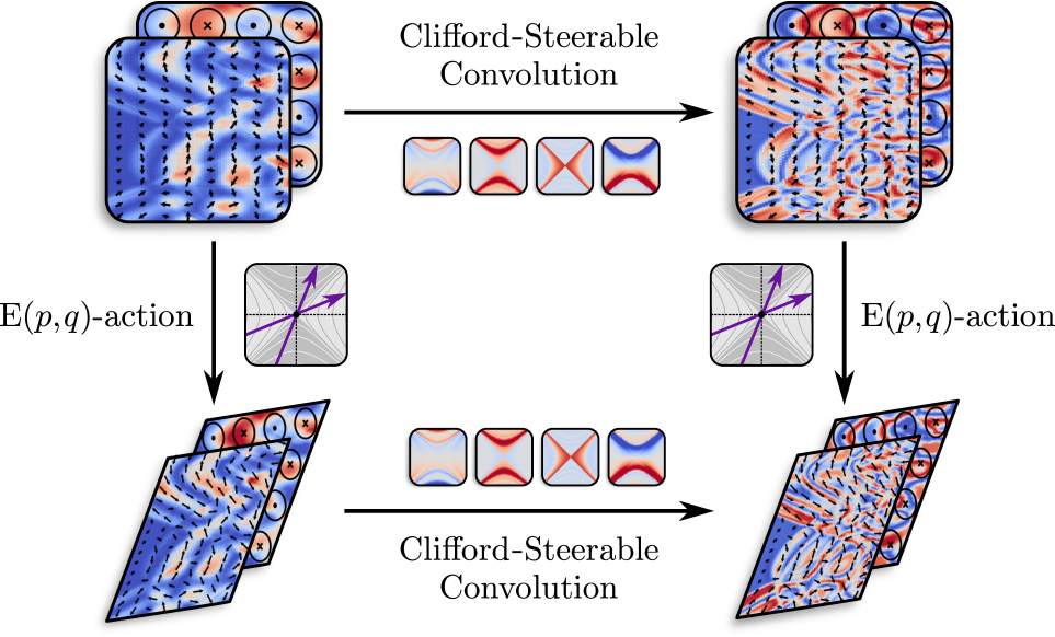
Figure 1: CS-CNNs process multivector fields while respecting $\operatorname{E}(p,q)$-equivariance. Shown here is a Lorentz-boost $\operatorname{O}(1,1)$ of electromagnetic data on 1+1-dimensional spacetime $\mathbb{R}^{1,1}$.

A fairly general class of equivariant CNNs covering arbitrary spaces and field types is described by the theory of steerable CNNs (Weiler et al., 2023). The central result there is that equivariance requires a “$G$-steerability” constraint on convolution kernels, where $G=\operatorname{O}(n)$ or $\operatorname{O}(p,q)$ for $\operatorname{E}(n)$- or $\operatorname{E}(p,q)$-equivariant CNNs, respectively. This constraint was solved and implemented for $\operatorname{O}(n)$ (Lang & Weiler, 2020; Cesa et al., 2022), however, $\operatorname{O}(p,q)$-steerable kernels are so far still missing.

This work proposes Clifford-steerable CNNs (CS-CNNs), which process multivector fields on pseudo-Euclidean spaces $\mathbb{R}^{p,q}$, and are equivariant to the pseudo-Euclidean group $\operatorname{E}(p,q)$: the isometries of $\mathbb{R}^{p,q}$. Multivectors are elements of the Clifford (or geometric) algebra $\operatorname{Cl}(\mathbb{R}^{p,q})$ of $\mathbb{R}^{p,q}$. Neural networks based on Clifford algebras have seen a recent surge in popularity in the field of deep learning and were used to build both non-equivariant (Brandstetter et al., 2023; Ruhe et al., 2023b) and equivariant (Ruhe et al., 2023a; Brehmer et al., 2023; Liu et al., 2024) models.

The steerability constraint on convolution kernels is usually either solved analytically or numerically, however, such solutions are not yet known for $\operatorname{O}(p,q)$. Observing that the $G$-steerability constraint is just a $G$-equivariance constraint, Zhdanov et al. (2022) propose to implement $G$-steerable kernels implicitly via $G$-equivariant MLPs. Our CS-CNNs follow this approach, implementing implicit $\operatorname{O}(p,q)$-steerable kernels via the $\operatorname{O}(p,q)$-equivariant neural networks for multivectors developed by Ruhe et al. (2023a).

We demonstrate the efficacy of our approach for predicting the evolution of several physical systems. In particular, we consider a fluid dynamics forecasting task on $\mathbb{R}^{2}$, as well as relativistic electrodynamics simulations on $\mathbb{R}^{3}$ and $\mathbb{R}^{1,2}$. CS-CNNs are the first models respecting the full spacetime symmetries of these problems. They significantly outperform competitive baselines, including conventional steerable CNNs and non-equivariant Clifford CNNs. This result remains consistent over dataset sizes. When evaluating the empirical equivariance error of our approach for $\operatorname{E}(2)$ symmetries, we find that we perform on par with the analytical solutions of Weiler & Cesa (2019).

This paper is organized as follows. Section 2 introduces the theoretical background on which CS-CNNs rely. Our approach itself is then developed in Section 3, and empirically evaluated in Section 4. A generalization of CS-CNNs from flat spacetimes to general pseudo-Riemannian manifolds is presented in Appendix F.

2 Theoretical Background

The core contribution of this work is to provide a framework for the construction of steerable CNNs for processing multivector fields on general pseudo-Euclidean spaces. We provide background on pseudo-Euclidean spaces and their symmetries in Section 2.1, on equivariant (steerable) CNNs in Section 2.2, and on multivectors and the Clifford algebra formed by them in Section 2.3.

2.1 Pseudo-Euclidean spaces and groups

Conventional Euclidean spaces are metric spaces, that is, they are equipped with a metric that assigns positive distances to any pair of distinct points. Pseudo-Euclidean spaces allow for more general indefinite metrics, which relax the positivity requirement on distances. Pseudo-Euclidean spaces appear in our theory in two distinct settings. First, the (affine) base spaces on which feature vector fields are supported, e.g. Minkowski spacetime, are pseudo-Euclidean. Second, the feature vectors attached to each point of spacetime are themselves elements of pseudo-Euclidean vector spaces. We introduce these spaces and their symmetries in the following.

2.1.1 Pseudo-Euclidean vector spaces

Definition 2.1 (Pseudo-Euclidean vector space).

A pseudo-Euclidean vector space (inner product space) $(V,\eta)$ of signature $(p,q)$ is a ${p\mkern-1.5mu+\mkern-2.0muq}$-dimensional vector space $V$ over $\mathbb{R}$ equipped with an inner product $\eta$, which we define as a non-degenerate symmetric bilinear form

$$\eta:\,V\times V \to\mathbb{R}, (v_{1},v_{2}) \mapsto\eta(v_{1},v_{2})$$ (1)

with $p$ and $q$ positive and negative eigenvalues, respectively.

If ${q\mkern-2.0mu=\mkern-2.0mu0}$, $\eta$ becomes positive-definite, and ${(V,\eta)}$ is a conventional Euclidean inner product space. For ${q\geq 1}$, ${\eta(v,v)}$ can be negative, rendering ${(V,\eta)}$ pseudo-Euclidean.

Since every inner product space $(V,\eta)$ of signature $(p,q)$ has an orthonormal basis, we can always find a linear isometry with the standard pseudo-Euclidean space $\mathbb{R}^{p,q}\cong(V,\eta)$, to which we mostly will restrict our attention in this paper:

Definition 2.2 (Standard pseudo-Euclidean vector spaces).

Let $e_{1},\dots,e_{p+q}$ be the standard basis of $\mathbb{R}^{p+q}$ and define an inner product of signature $(p,q)$

$$\eta^{p,q}(v_{1},v_{2})\,:=\,v_{1}^{\top}\Delta^{p,q}v_{2}$$ (2)

in this basis via its matrix representation

$$\Delta^{p,q}:=\mathrm{diag}(\underbrace{1,\dots,1\vphantom{\big{|}}}_{\textup{$p$ times}},\,\underbrace{\scalebox{0.75}[1.0]{$-$}1,\dots,\scalebox{0.75}[1.0]{$-$}1\vphantom{\big{|}}}_{\textup{$q$ times}})\,.$$ (3)

We call the inner product space $\mathbb{R}^{p,q}:=(\mathbb{R}^{p+q},\eta^{p,q})$ the standard pseudo-Euclidean vector space of signature $(p,q)$.

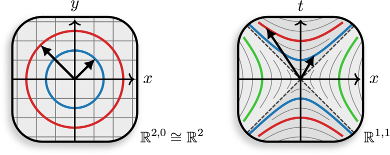
Figure 2: Examples of pseudo-Euclidean spaces $\mathbb{R}^{2,0}$ and $\mathbb{R}^{1,1}$. Colors depict $\operatorname{O}(p,q)$-orbits, given by sets of all points $v\in\mathbb{R}^{p,q}$ with the same squared distance $\eta^{p,q}(v,v)$ from the origin.

Example 2.3.

${\mathbb{R}^{3,0}\equiv\mathbb{R}^{3}}$ recovers the 3-dimensional Euclidean vector space with its standard positive-definite inner product $\Delta^{3,0}=\mathrm{diag}(1,1,1)$. The signature ${(p,q)}={(1,3)}$ corresponds, instead, to Minkowski spacetime $\mathbb{R}^{1,3}$ with Minkowski inner product $\Delta^{1,3}=\mathrm{diag}(1,\scalebox{0.75}[1.0]{$-$}1,\scalebox{0.75}[1.0]{$-$}1,\scalebox{0.75}[1.0]{$-$}1)$ .

2.1.2 Pseudo-Euclidean groups

We are interested in neural networks that respect (i.e., commute with, or are equivariant to) the symmetries of pseudo-Euclidean spaces, which we define here. For concreteness, we give these definitions for the standard pseudo-Euclidean vector spaces $\mathbb{R}^{p,q}$. Let us start with the two cornerstone groups that define such symmetries:

Definition 2.4 (Translation groups).

The translation group $(\mathbb{R}^{p,q},+)$ associated with $\mathbb{R}^{p,q}$ is formed by its set of vectors and its (canonical) vector addition.

Definition 2.5 (Pseudo-orthogonal groups).

The pseudo-orthogonal group $\operatorname{O}(p,\mkern-1.0muq)$ associated to $\mathbb{R}^{p,q}$ is formed by all invertible linear maps that preserve its inner product,

$$\operatorname{O}(p,q)\,:=\,\big{\{}g\in\operatorname{GL}(\mathbb{R}^{p,q})\,\big{|}\,g^{\top}\!\Delta^{p,q}g=\Delta^{p,q}\big{\}},$$ (4)

together with matrix multiplication. $\operatorname{O}(p,q)$ is compact for ${p=0}$ or ${q=0}$, and non-compact for mixed signatures.

Example 2.6.

For ${(p,q)=(3,0)}$, we obtain the usual orthogonal group $\operatorname{O}(3)$, i.e. rotations and reflections, while ${(p,q)=(1,3)}$ corresponds to the relativistic Lorentz group $\operatorname{O}(1,3)$, which also includes boosts between inertial frames.

Taken together, translations and pseudo-orthogonal transformations of $\mathbb{R}^{p,q}$ form its pseudo-Euclidean group, which is the group of all metric preserving symmetries (isometries).

Definition 2.7 (Pseudo-Euclidean groups).

The pseudo-Euclidean group for $\mathbb{R}^{p,q}$ is defined as semidirect product

$$\operatorname{E}(p,q)\,:=\,(\mathbb{R}^{p,q},+)\rtimes\operatorname{O}(p,q)$$ (5)

with group multiplication defined by ${(\tilde{t},\mkern-2.0mu\tilde{g})\cdot(t,\mkern-2.0mug)}={(\tilde{t}+\tilde{g}t,}\,\tilde{g}g)$. Its canonical action on $\mathbb{R}^{p,q}$ is given by

$$\operatorname{E}(p,q)\times\mathbb{R}^{p,q}\to\mathbb{R}^{p,q},\quad\big{(}(t,\mkern-2.0mug),\,x\big{)}\mapsto gx+t$$ (6)

Example 2.8.

The usual Euclidean group $\operatorname{E}(3)$ is reproduced for ${(p,q)=(3,0)}$. For Minkowski spacetime, ${(p,q)=(1,3)}$, we obtain the Poincaré group $\operatorname{E}(1,3)$.

2.2 Feature vector fields & Steerable CNNs

Convolutional neural networks operate on spatial signals, formalized as fields of feature vectors on a base space $\mathbb{R}^{p,q}$. Transformations of the base space imply corresponding transformations of the feature vector fields defined on them, see Fig. 1 (left column). The specific transformation laws depend thereby on their geometric “field type” (e.g., scalar, vector, or tensor fields). Equivariant CNNs commute with such transformations of feature fields. The theory of steerable CNNs shows that this requires a $G$-equivariance constraint on convolution kernels (Weiler et al., 2023). We briefly review the definitions and basic results of feature fields and steerable CNNs in Sections 2.2.1 and 2.2.2 below.

For generality, this section considers arbitrary matrix groups $G\leq\operatorname{GL}(\mathbb{R}^{p,q})$ and affine groups $\mathrm{Aff}(G)=(\mathbb{R}^{p,q},+)\rtimes G$, and allows for any field type. Section 3 will more specifically focus on pseudo-orthogonal groups $G=\operatorname{O}(p,q)$, pseudo-Euclidean groups $\mathrm{Aff}(\operatorname{O}(p,q))=\operatorname{E}(p,q)$, and multivector fields. For a detailed review of Euclidean steerable CNNs and their generalization to Riemannian manifolds we refer to Weiler et al. (2023).

2.2.1 Feature vector fields

Feature vector fields are functions ${f:\mathbb{R}^{p,q}\to W}$ that assign to each point $x\in\mathbb{R}^{p,q}$ a feature $f(x)$ in some feature vector space $W$. They are additionally equipped with an $\mathrm{Aff}(G)$-action determined by a $G$-representation $\rho$ on $W$.

The specific choice of $(W,\rho)$ fixes the geometric “type” of feature vectors. For instance, $W=\mathbb{R}$ and trivial $\rho(g)=1$ corresponds to scalars, $W=\mathbb{R}^{p,q}$ and $\rho(g)=g$ describes tangent vectors. Higher order tensor spaces and representations give rise to tensor fields. Later on, ${W\mkern-3.0mu=\mkern-1.0mu\operatorname{Cl}(\mathbb{R}^{p,q})}$ will be the Clifford algebra and feature vectors will be multivectors with a natural $\operatorname{O}(p,q)$-representation $\rho_{\operatorname{Cl}}$.

Definition 2.9 (Feature vector field).

Consider a pseudo-Euclidean “base space” $\mathbb{R}^{p,q}$. Fix any $G\leq\operatorname{GL}(\mathbb{R}^{p,q})$ and consider a $G$-representation $(W,\rho)$, called “field type”.

Let ${\Gamma(\mathbb{R}^{p,q},W):=\{f:\mathbb{R}^{p,q}\to W\}}$ denote the vector space of $W$​-feature fields. Define an $\mathrm{Aff}(G)$-action

$$\rhd_{\rho}:\mathrm{Aff}(G)\times\Gamma(\mathbb{R}^{p,q},W)\to\Gamma(\mathbb{R}^{p,q},W)$$ (7)

by setting, for any $(t,\mkern-2.0mug)\in\mathrm{Aff}(G)$, any $f\in\Gamma(\mathbb{R}^{p,q},W)$, and $x\in\mathbb{R}^{p,q}$,

$$\big{[}(t,\mkern-2.0mug)\mkern-2.0mu\rhd_{\rho}\mkern-3.0muf\big{]}(x):=\rho(g)f\big{(}(t,\mkern-2.0mug)^{\scalebox{0.75}[1.0]{$-$}1}x\big{)}=\rho(g)f\big{(}g^{\scalebox{0.75}[1.0]{$-$}1}(x\scalebox{0.75}[1.0]{$-$}t)\big{)}.$$

Since $\Gamma(\mathbb{R}^{p,q},W)$ is a vector space and $\rhd_{\rho}$ is linear, the tuple $\big{(}\Gamma(\mathbb{R}^{p,q},W),\rhd_{\rho}\big{)}$ forms the $\mathrm{Aff}(G)$-representation of feature vector fields of type $(W,\rho)$.

Remark 2.10.

Intuitively, $(t,\mkern-2.0mug)$ acts on $f$ by

1. moving feature vectors across the base space, from points $g^{-1}(x-t)$ to new locations $x$, and

2. $G$-transforming individual feature vectors $f(x)\in W$ themselves by means of the $G$-representation $\rho(g)$.

Besides the field types mentioned above, equivariant neural networks often rely on irreducible, regular or quotient representations. More choices of field types are discussed and benchmarked in Weiler & Cesa (2019).

2.2.2 Steerable CNNs

Steerable convolutional neural networks are composed of layers that are $\mathrm{Aff}(G)$-equivariant, that is, which commute with affine group actions on feature fields:

Definition 2.11 ($\mathrm{Aff}(G)$-equivariance).

Consider any two $G$-representations $(W_{\textup{in}},\rho_{\textup{in}})$ and $(W_{\textup{out}},\rho_{\textup{out}})$. Let $L:\Gamma(\mathbb{R}^{p,q},W_{\textup{in}})\to\Gamma(\mathbb{R}^{p,q},W_{\textup{out}})$ be a function (“layer”) between the corresponding spaces of feature fields. This layer is said to be $\mathrm{Aff}(G)$-equivariant iff it satisfies

$$L\big{(}(t,\mkern-2.0mug)\rhd_{\rho_{\textup{in}}}f\big{)}\,=\,(t,\mkern-2.0mug)\rhd_{\rho_{\textup{out}}}L(f)$$ (8)

for any $(t,\mkern-2.0mug)\in\mathrm{Aff}(G)$ and any $f\in\Gamma(\mathbb{R}^{p,q},W_{\textup{in}})$. Equivalently, the following diagram should commute:

(9)

The most basic operations used in neural networks are parameterized linear layers. If one demands translation equivariance, these layers are necessarily convolutions (Weiler et al., 2023)[Theorem 3.2.1]. Similarly, linearity and $\mathrm{Aff}(G)$-equivariance requires steerable convolutions, that is, convolutions with $G$-steerable kernels:

Theorem 2.12 (Steerable convolution).

Consider a layer ${L:\Gamma(\mathbb{R}^{p,q},W_{\textup{in}})\to\Gamma(\mathbb{R}^{p,q},W_{\textup{out}})}$ mapping between feature fields of types $(W_{\textup{in}},\rho_{\textup{in}})$ and $(W_{\textup{out}},\rho_{\textup{out}})$, respectively. If $L$ is demanded to be linear and $\mathrm{Aff}(G)$-equivariant, then:

1. $L$ needs to be a convolution integral

   $$L\mkern-1.0mu\big{(}f_{\mathrm{in}}\big{)}(u)\mkern 1.0mu=\mkern 1.0mu\big{[}K\mkern-2.0mu\ast\mkern-2.0muf_{\mathrm{in}}\big{]}\mkern-2.0mu(u)\mkern 1.0mu:=\mkern-2.0mu\int_{\mathbb{R}^{p,q}}\mkern-18.0muK(v)\big{[}f_{\mathrm{in}}(u\scalebox{0.75}[1.0]{$-$}v)\big{]}\mkern 2.0mudv,$$

   parameterized by a convolution kernel

   $$K:\mathbb{R}^{p,q}\to\operatorname{Hom}_{\mathrm{Vec}}(W_{\textup{in}},W_{\textup{out}})\,.$$ (10)

   The kernel is operator-valued since it aggregates input features in $W_{\textup{in}}$ linearly into output features in $W_{\textup{out}}$.

2. The kernel is required to be $G$-steerable, that is, it needs to satisfy the $G$-equivariance constraint

   $$K(gx)\ =\ \scalebox{0.875}{$\displaystyle\frac{1}{|\det(g)|}$}\rho_{\textup{out}}(g)K(x)\rho_{\textup{in}}(g)^{-1}$$ (11)

   $$=:\ \rho_{\textup{Hom}}(g)(K(x))$$

   for any $g\in G$ and $x\in\mathbb{R}^{p,q}$. This constraint is diagrammatically visualized by the commutativity of:

   (12)

Proof.

See (Weiler et al., 2023)[Theorem 4.3.1]. ∎

Remark 2.13 (Discretized kernels).

In practice, kernels are often discretized as arrays of shape

$$\big{(}X_{1},\dots,X_{p+q},\,C_{\textup{out}},C_{\textup{in}}\big{)}$$

with ${C_{\textup{out}}\mkern-1.0mu=\mkern-1.0mu\dim(W_{\textup{out}})}$ and ${C_{\textup{in}}\mkern-1.0mu=\mkern-1.0mu\dim(W_{\textup{in}})}$. The first $p+q$ axes are hereby indexing a pixel grid on the domain $\mathbb{R}^{p,q}$, while the last two axes represent the linear operators in the codomain by ${C_{\textup{out}}\mkern-2.0mu\times\mkern-2.0muC_{\textup{in}}}$ matrices.

The main takeaway of this section is that one needs to implement $G$-steerable kernels in order to implement $\mathrm{Aff}(G)$-equivariant CNNs. This is a notoriously difficult problem, requiring specialized approaches for different categories of groups $G$ and field types $(W,\rho)$. Unfortunately, the usual approaches do not immediately apply to our goal of implementing $\operatorname{O}(p,q)$-steerable kernels for multivector fields. These include the following cases:

• Most commonly, steerable kernels are parameterized in analytically derived steerable kernel bases. Solutions are known for $\operatorname{SO}(3)$ (Weiler et al., 2018a), $\operatorname{O}(3)$ (Geiger et al., 2020) and any $G\leq\operatorname{O}(2)$ (Weiler & Cesa, 2019). Lang & Weiler (2020) and Cesa et al. (2022) generalized this to any compact groups ${G\mkern-2.0mu\leq\mkern-2.0mu\operatorname{U}(d)}$. However, their solutions still require knowledge of irreps, Clebsch-Gordan coefficients and harmonic basis functions, which need to be derived and implemented for each single group individually. Furthermore, these solutions do not cover pseudo-orthogonal groups $\operatorname{O}(p,q)$ of mixed signature, since these are non-compact.

• For regular and quotient representations, steerable kernels can be implemented via channel permutations in the matrix dimensions. This is, for instance, done in regular group convolutions (Cohen & Welling, 2016; Weiler et al., 2018b; Bekkers et al., 2018; Cohen et al., 2019b; Finzi et al., 2020). However, these approaches require finite $G$ or rely on sampling compact $G$, again ruling out general (non-compact) $\operatorname{O}(p,q)$.

• Cohen & Welling (2017) solved the kernel constraint for finite $G$ numerically. For $\operatorname{SO}(2)$, de Haan et al. (2021) derived numerical solutions based on Lie-algebra representation theory. The numerical routine by Shutty & Wierzynski (2022) solves for Lie-algebra irreps given their structure constants. Corresponding Lie group irreps follow via the matrix exponential, however, only on connected groups like the subgroups $\operatorname{SO}^{+}(p,q)$ of $\operatorname{O}(p,q)$.

• Steerable kernels are merely $G$-equivariant maps between vector spaces $\mathbb{R}^{p,q}$ and $\operatorname{Hom}_{\mathrm{Vec}}(W_{\textup{in}},W_{\textup{out}})$. Based on this insight, Zhdanov et al. (2022) parameterize them implicitly via $G$-equivariant MLPs. However, to implement these MLPs, one usually requires irreps, irrep endomorphisms and Clebsch-Gordan coefficients for each $G$ of interest.

Our approach presented in Section 3 is based on the implicit kernel parametrization via neural networks by Zhdanov et al. (2022), which requires us to implement $\operatorname{O}(p,q)$-equivariant neural networks. Fortunately, the Clifford group equivariant neural networks by Ruhe et al. (2023a) establish $\operatorname{O}(p,q)$-equivariance for the practically relevant case of Clifford-algebra representations $\rho_{\operatorname{Cl}}$, i.e., $\operatorname{O}(p,q)$-actions on multivectors. The Clifford algebra, and Clifford group equivariant neural networks, are introduced in the next section.

2.3 The Clifford Algebra & Clifford Group Equivariant Neural Networks

This section introduces multivector features, a specific type of geometric feature vectors with $\operatorname{O}(p,q)$-action. Multivectors are the elements of a Clifford algebra $\operatorname{Cl}(V,\eta)$ corresponding to a pseudo-Euclidean $\mathbb{R}$-vector space $(V,\eta)$. The most relevant properties of Clifford algebras in relation to applications in geometric deep learning are the following:

• $\operatorname{Cl}(V,\eta)$ is, in itself, an $\mathbb{R}$-vector space of dimension $2^{d}$ with $d:=\dim(V)={p\mkern-1.0mu+\mkern-1.0muq}$. This allows to use multivectors as feature vectors of neural networks (Brandstetter et al., 2023; Ruhe et al., 2023b; Brehmer et al., 2023).

• As an algebra, ${\operatorname{Cl}(\mkern-0.5muV,\mkern-1.5mu\eta)}$ comes with an $\mathbb{R}$-bilinear operation

  $$\mathbin{\ThisStyle{\vbox{\hbox{\scalebox{0.65}{$\SavedStyle\bullet$}}}}}:\;\operatorname{Cl}(V,\eta)\mkern-1.0mu\times\mkern-1.0mu\operatorname{Cl}(V,\eta)\,\to\,\operatorname{Cl}(V,\eta)$$

  called geometric product. We can therefore multiply multivectors with each other, which will be a key aspect in various neural network operations.

• $\operatorname{Cl}(V,\eta)$ is furthermore a representation space of the pseudo-orthogonal group $\operatorname{O}(V,\eta)$ via $\rho_{\operatorname{Cl}}$, defined in Eq (LABEL:eq:pseudo_orthogonal_group_abstract) below. This allows to use multivectors as features of $\operatorname{O}(V,\eta)$-equivariant networks (Ruhe et al., 2023a).

  A formal definition of Clifford algebras can be found in Appendix D. Section 2.3.1 offers a less technical introduction, highlighting basic constructions and results. Sections 2.3.2 and 2.3.3 focus on the natural $\operatorname{O}(p,q)$-action on multivectors, and on Clifford group equivariant neural networks. While we will later mostly be interested in $(V,\eta)\mkern-2.0mu=\mkern-1.0mu\mathbb{R}^{p,q}$ and $\operatorname{O}(V,\eta)=\operatorname{O}(p,q)$, we keep the discussion here general.

  2.3.1 Introduction to the Clifford algebra

  Multivectors are constructed by multiplying and summing vectors. Specifically, $l$ vectors $v_{1},\dots,v_{l}\in V$ multiply to ${v_{1}\mathbin{\ThisStyle{\vbox{\hbox{\scalebox{0.65}{$\SavedStyle\bullet$}}}}}\dots\mathbin{\ThisStyle{\vbox{\hbox{\scalebox{0.65}{$\SavedStyle\bullet$}}}}}v_{l}}\in\operatorname{Cl}(V,\eta)$. A general multivector arises as a linear combination of such products,

  $$x=\sum\nolimits_{i\in I}c_{i}\cdot v_{i,1}\mathbin{\ThisStyle{\vbox{\hbox{\scalebox{0.65}{$\SavedStyle\bullet$}}}}}\cdots\mathbin{\ThisStyle{\vbox{\hbox{\scalebox{0.65}{$\SavedStyle\bullet$}}}}}v_{i,l_{i}}\,,$$ (13)

  with some finite index set $I$ and $v_{i,k}\in V$ and $c_{i}\in\mathbb{R}$.

  The main algebraic property of the Clifford algebra is that it relates the geometric product of vectors $v\in V$ to the inner product $\eta$ on $V$ by requiring:

  $$v\mathbin{\ThisStyle{\vbox{\hbox{\scalebox{0.65}{$\SavedStyle\bullet$}}}}}v\,\overset{!}{=}\,\eta(v,v)\cdot 1_{\operatorname{Cl}(V,\eta)}\qquad\forall\,v\in V\subset\operatorname{Cl}(V,\eta)$$ (14)

  Intuitively, this means that the product of a vector with itself collapses to a scalar value $\eta(v,v)\in\mathbb{R}\subseteq\operatorname{Cl}(V,\eta)$, from which all other properties of the algebra follow by bilinearity. This leads in particular to the fundamental relation:

  $$v_{2}\mathbin{\ThisStyle{\vbox{\hbox{\scalebox{0.65}{$\SavedStyle\bullet$}}}}}v_{1}=-v_{1}\mathbin{\ThisStyle{\vbox{\hbox{\scalebox{0.65}{$\SavedStyle\bullet$}}}}}v_{2}\,+\,2\eta(v_{1},v_{2})\!\cdot\!1_{\operatorname{Cl}(V,\eta)}\quad\forall\,v_{1},v_{2}\in V.$$

  For the standard orthonormal basis $[e_{1},\dots,e_{p+q}]$ of $\mathbb{R}^{p,q}$ this reduces to the following simple rules:

  $$e_{i}\mathbin{\ThisStyle{\vbox{\hbox{\scalebox{0.65}{$\SavedStyle\bullet$}}}}}e_{j}\,=\, -e_{j}\mathbin{\ThisStyle{\vbox{\hbox{\scalebox{0.65}{$\SavedStyle\bullet$}}}}}e_{i} i\neq j$$ for (15a)

  $$e_{i}\mathbin{\ThisStyle{\vbox{\hbox{\scalebox{0.65}{$\SavedStyle\bullet$}}}}}e_{j}\,=\, \eta(e_{i},e_{i})=+1 i=j\leq p$$ for (15b)

  $$e_{i}\mathbin{\ThisStyle{\vbox{\hbox{\scalebox{0.65}{$\SavedStyle\bullet$}}}}}e_{j}\,=\, \eta(e_{i},e_{i})=-1 i=j>p$$ for (15c)

  An (orthonormal) basis of $\operatorname{Cl}(V,\eta)$ is constructed by repeatedly taking geometric products of any basis vectors $e_{i}\in V$. Note that, up to sign flip, (1) the ordering of elements in any product is irrelevant due to Eq. (15a), and (2) any elements occurring twice cancel out due to Eqs. (15b,15c).

  name	grade $k$	dim ${d\choose k}$	basis $k$-vectors	​norm​
  scalar	$0$	$1$	$1$	$+1$
  vector	$1$	$3$	$e_{1}$	$+1$
  			$e_{2},\;e_{3}$	$-1$
  ​pseudovector	$2$	$3$	$e_{12},\;e_{13}$	$-1$
  			$e_{23}$	$+1$
  ​pseudoscalar	$3$	$1$	$e_{123}$	$+1$

  Table 1: Orthonormal basis for $\operatorname{Cl}(\mathbb{R}^{p,q})$ with $(p,q)=(1,2)$. “Norm” refers to $\bar{\eta}(e_{A},e_{A})=\eta_{A}$; see Eq. (18).

  The basis elements constructed this way can be identified with (and labeled by) subsets $A\subseteq[d]:=\{1,\dots,d\}$, where the presence or absence of an index $i\in A$ signifies whether the corresponding $e_{i}$ appears in the product. Agreeing furthermore on an ordering to disambiguate signs, we define

  $$e_{A}:=e_{i_{1}}\!\mathbin{\ThisStyle{\vbox{\hbox{\scalebox{0.65}{$\SavedStyle\bullet$}}}}}e_{i_{2}}\!\mathbin{\ThisStyle{\vbox{\hbox{\scalebox{0.65}{$\SavedStyle\bullet$}}}}}\dots\mathbin{\ThisStyle{\vbox{\hbox{\scalebox{0.65}{$\SavedStyle\bullet$}}}}}e_{i_{k}}\mkern 15.0mu\textup{for }\ A=\{i_{1}\mkern-2.0mu<\mkern-2.0mu\cdots\mkern-2.0mu<\mkern-2.0mui_{k}\}\neq\varnothing$$

  and ${e_{\varnothing}:=1_{\operatorname{Cl}(V,\eta)}}$. From this, it is clear that $\dim\operatorname{Cl}(V,\eta)$ $=2^{d}$. Table 1 gives a specific example for $(V,\eta)=\mathbb{R}^{1,2}$.

  Any multivector $x\in\operatorname{Cl}(V,\eta)$ can be uniquely expanded in this basis,

  $$x\,=\,\sum\nolimits_{A\subseteq[d]}x_{A}\cdot e_{A},$$ (16)

  where $x_{A}\in\mathbb{R}$ are coefficients.

  Note that there are $\binom{d}{k}$ basis elements $e_{A}$ of “grade” ${|\mkern-1.0muA|\mkern-3.0mu=\mkern-3.0muk}$, i.e., which are composed from $k$ out of the $d$ distinct $e_{i}\in V$. These span ${d\mkern-2.0mu+\mkern-2.0mu1}$ linear subspaces $\operatorname{Cl}^{(k)}(V,\eta)$, the elements of which are called $k$-vectors. They include scalars (${k\mkern-2.0mu=\mkern-2.0mu0}$), vectors (${k\mkern-2.0mu=\mkern-2.0mu1}$), bivectors (${k\mkern-2.0mu=\mkern-2.0mu2}$), etc. The full Clifford algebra decomposes thus into a direct sum over grades:

  $$\operatorname{Cl}(V,\eta)=\bigoplus_{k=0}^{d}\operatorname{Cl}^{(k)}(V,\eta),\mkern 16.0mu\dim\operatorname{Cl}^{(k)}(V,\eta)\mkern-1.0mu=\mkern-1.0mu\binom{d}{k}.$$

  Given any multivector $x$, expanded as in Eq. (16), we can define its $k$-th grade projection on $\operatorname{Cl}^{(k)}(V,\eta)$ as:

  $$x^{(k)}\,=\,\sum\nolimits_{A\subseteq[d],\,|A|=k}x_{A}\cdot e_{A}.$$ (17)

  Finally, the inner product $\eta$ on $V$ is naturally extended to $\operatorname{Cl}(V,\eta)$ by defining $\bar{\eta}:\operatorname{Cl}(V,\eta)\times\operatorname{Cl}(V,\eta)\to\mathbb{R}$ as

  $$\bar{\eta}(x,y)\,:=\,\sum\nolimits_{A\subseteq[d]}\eta_{A}\cdot x_{A}\cdot y_{A},$$ (18)

  where $\eta_{A}:=\prod\nolimits_{i\in A}\eta(e_{i},\!e_{i})\in\{\pm 1\}$ are sign factors. The tuple $(e_{A})_{A\subseteq[d]}$ is an orthonormal basis of $\operatorname{Cl}(V,\eta)$ w.r.t. $\bar{\eta}$.

  All of these constructions and statements are more formally defined and proven in the appendix of (Ruhe et al., 2023b).

  2.3.2 Clifford grades as $\operatorname{O}\mkern-0.5mu(p,\mkern-2.0muq\mkern-0.5mu)$-representations

  The individual grades $\operatorname{Cl}^{(k)}(V,\eta)$ turn out to be representation spaces of the (abstract) pseudo-orthogonal group

  $$\mkern-6.0mu\operatorname{O}(V,\eta):=\big{\{}g\mkern-1.0mu\in\mkern-1.0mu\operatorname{GL}(V)\mkern 2.0mu\big{|}\,\forall v\mkern-3.0mu\in\mkern-3.0muV\!:\eta(gv,\mkern-2.0mugv)\mkern-2.0mu=\mkern-2.0mu\eta(v,\mkern-2.0muv)\mkern-1.0mu\big{\}},$$

  which coincides for $(V,\eta)=\mathbb{R}^{p,q}$ with $\operatorname{O}(p,q)$ in Def. 2.2. $\operatorname{O}(V,\eta)$ acts thereby on multivectors by individually multiplying each $1\mkern-1.0mu$-vector from which they are constructed with $g$.

  Definition/Theorem 2.14 ($\operatorname{O}(V,\eta)$-action on $\operatorname{Cl}(V,\eta)$).

  Let $(V,\eta)$ be a pseudo-Euclidean space, $g,g_{i}\in\operatorname{O}(V,\eta)$, $c_{i}\in\mathbb{R}$, $v_{i,j}\in V$, $x,x_{i}\in\operatorname{Cl}(V,\eta)$, and $I$ a finite index set.
  Define the orthogonal algebra representation

  $$\rho_{\operatorname{Cl}}:\,\operatorname{O}(V,\eta)\to\operatorname{O}_{\operatorname{Alg}}\left(\operatorname{Cl}(V,\eta),\bar{\eta}\right)$$ (20)

  of $\operatorname{O}(V,\eta)$ via the canonical $\operatorname{O}(V,\eta)$-action on each of the contained $1$-vectors:

  $$\rho_{\operatorname{Cl}}(g)\Big{(}\sum\nolimits_{i\in I}c_{i}\mkern-2.0mu\cdot\mkern-2.0muv_{i1}\mathbin{\ThisStyle{\vbox{\hbox{\scalebox{0.65}{$\SavedStyle\bullet$}}}}}\ldots\mathbin{\ThisStyle{\vbox{\hbox{\scalebox{0.65}{$\SavedStyle\bullet$}}}}}v_{ij_{i}}\Big{)}$$ (21)

  $$\mkern 0.0mu:= \sum\nolimits_{i\in I}c_{i}\mkern-2.0mu\cdot\mkern-2.0mu(gv_{i1})\mathbin{\ThisStyle{\vbox{\hbox{\scalebox{0.65}{$\SavedStyle\bullet$}}}}}\ldots\mathbin{\ThisStyle{\vbox{\hbox{\scalebox{0.65}{$\SavedStyle\bullet$}}}}}(gv_{ij_{i}}).$$

  $\rho_{\operatorname{Cl}}$ is well-defined as an orthogonal representation:

  • $\mkern 8.0mu\rho_{\operatorname{Cl}}(g)(c_{1}\cdot x_{1}+c_{2}\cdot x_{2})$
    $=c_{1}\cdot\rho_{\operatorname{Cl}}(g)(x_{1})+c_{2}\cdot\rho_{\operatorname{Cl}}(g)(x_{2})$

  • $\mkern 8.0mu\rho_{\operatorname{Cl}}(g_{2})\left(\rho_{\operatorname{Cl}}(g_{1})(x)\right)=\rho_{\operatorname{Cl}}(g_{2}g_{1})(x)$

  • $\mkern 8.0mu\rho_{\operatorname{Cl}}(g)^{-1}(x)=\rho_{\operatorname{Cl}}(g^{-1})(x)$,

  • $\mkern 8.0mu\bar{\eta}(\rho_{\operatorname{Cl}}(g)(x_{1}),\rho_{\operatorname{Cl}}(g)(x_{2}))=\bar{\eta}(x_{1},x_{2})$

  Moreover, the geometric product is $\operatorname{O}(V,\eta)$-equivariant, making $\rho_{\operatorname{Cl}}$ an (orthogonal) algebra representation:

  $$\rho_{\operatorname{Cl}}(g)(x_{1})\mathbin{\ThisStyle{\vbox{\hbox{\scalebox{0.65}{$\SavedStyle\bullet$}}}}}\rho_{\operatorname{Cl}}(g)(x_{2})=\rho_{\operatorname{Cl}}(g)(x_{1}\mathbin{\ThisStyle{\vbox{\hbox{\scalebox{0.65}{$\SavedStyle\bullet$}}}}}x_{2}).$$ (22)

  (23)

  This representation $\rho_{\operatorname{Cl}}$ reduces furthermore to independent sub-representations on individual $k$-vectors.

  Theorem 2.15 ($\operatorname{O}(V,\eta)$-action on grades $\operatorname{Cl}^{(k)}(V,\eta)$).

  Let $g\in\operatorname{O}(V,\eta)$, $x\in\operatorname{Cl}(V,\eta)$ and $k\in{0,\dots,d}$ a grade.
  The grade projection $(\mkern 2.0mu\cdot\mkern 2.0mu)^{(k)}$ is $\operatorname{O}(V,\eta)$-equivariant:

  $$\big{(}\rho_{\operatorname{Cl}}(g)\,x\big{)}^{(k)}=\rho_{\operatorname{Cl}}(g)\big{(}x^{(k)}\big{)}$$ (24)

  (25)

  This implies in particular that $\operatorname{Cl}(V,\eta)$ is reducible to subrepresentations $\operatorname{Cl}^{(k)}(V,\eta)$, i.e. $\rho_{\operatorname{Cl}}(g)$ does not mix grades.

  Proof.

  Both theorems are proven in (Ruhe et al., 2023a). ∎

  2.3.3 $\operatorname{O}\mkern-0.5mu(p,\mkern-2.0muq\mkern-0.5mu)$-equivariant Clifford Neural Nets

  Based on those properties, Ruhe et al. (2023a) proposed Clifford group equivariant neural networks (CGENNs). Due to a group isomorphism, this is equivalent to the network’s $\operatorname{O}(V,\eta)$-equivariance.

  Definition/Theorem 2.16 (Clifford Group Equivariant NN).

  Consider a grade ${k=0,\mkern-1.0mu...,d}$ and weights $w^{k}_{mn}\in\mathbb{R}$. A Clifford group equivariant neural network (CGENN) is constructed from the following functions, operating on one or more multivectors $x_{i}\in\operatorname{Cl}(V,\eta)$.

  • mix $k$-vectors. For each ${1\mkern-2.0mu\leq\mkern-2.0mum\mkern-2.0mu\leq\mkern-2.0mu{c_{\mathrm{out}}}}$:

    $$L_{m}^{(k)}(x_{1},\dots,x_{{c_{\mathrm{in}}}}):=\sum\nolimits_{n=1}^{{c_{\mathrm{in}}}}w_{mn}^{k}\cdot x_{n}^{(k)}$$ (26)

    Such weighted linear mixing within sub-representations $\operatorname{Cl}^{(k)}(V,\eta)$ is common in equivariant MLPs.

  • compute weighted geometric products with grade-dependent weights:

    $$P^{(k)}(x_{1},x_{2}):=\sum\nolimits_{m=0}^{d}\sum\nolimits_{n=0}^{d}w_{mn}^{k}\mkern-2.0mu\cdot\mkern-2.0mu\big{(}x_{1}^{(m)}\mathbin{\ThisStyle{\vbox{\hbox{\scalebox{0.65}{$\SavedStyle\bullet$}}}}}x_{2}^{(n)}\big{)}^{(k)}$$

    This is similar to the irrep-feature tensor products in MACE (Batatia et al., 2022).

  • As activations, we use ${A(x)\mkern-1.0mu:=\mkern-1.0mux\mkern-1.5mu\cdot\mkern-1.5mu\Phi\big{(}x^{(0)}\big{)}}$ where $\Phi$ is the CDF of the Gaussian distribution. This is inspired by $\mathrm{GatedGELU}$ from Brehmer et al. (2023).

  All of these operations are by Theorems 2.14 and 2.15 $\operatorname{O}(V,\eta)$-equivariant.

  

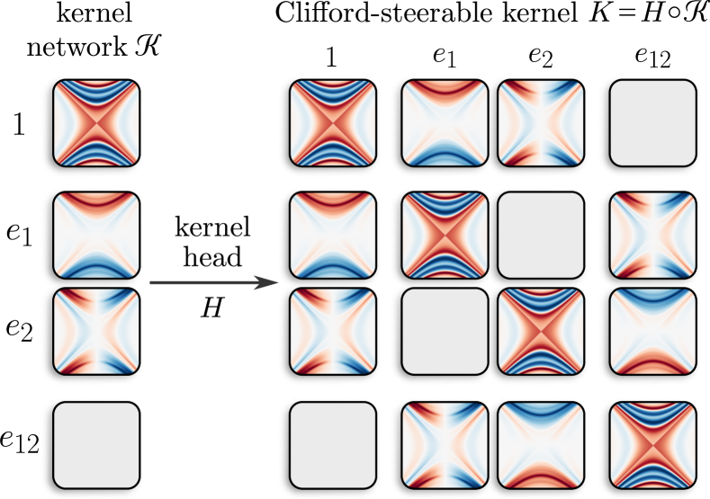
  Figure 3: Left: Multi-vector valued output of the kernel-network $\mathscr{K}$ for ${{c_{\mathrm{in}}}\mkern-2.0mu=\mkern-2.0mu{c_{\mathrm{out}}}\mkern-2.0mu=\mkern-2.0mu1,(p,\mkern-2.0muq)\mkern-2.0mu=\mkern-2.0mu(1,\mkern-2.0mu1)}$, and its expansion to a full ${\operatorname{O}(1,\mkern-3.0mu1)}$-steerable kernel via the kernel head $H$. Right: Commutative diagram of the construction and ${\operatorname{O}(p,\mkern-2.0muq)}$-equivariance of implicit steerable kernels ${K\mkern-3.0mu=\mkern-2.0muH\mkern-2.0mu\circ\mkern-2.0mu\mathscr{K}}$, composed from a kernel network $\mathscr{K}$ with ${{c_{\mathrm{out}}}\!\times\!{c_{\mathrm{in}}}}$ multivector outputs and the kernel head $H$. The two inner squares show the individual equivariance of $\mathscr{K}$ and $H$, from which the kernels’ overall equivariance follows. We abbreviate $\operatorname{Cl}(\mathbb{R}^{p,q})$ by $\operatorname{Cl}$.

  

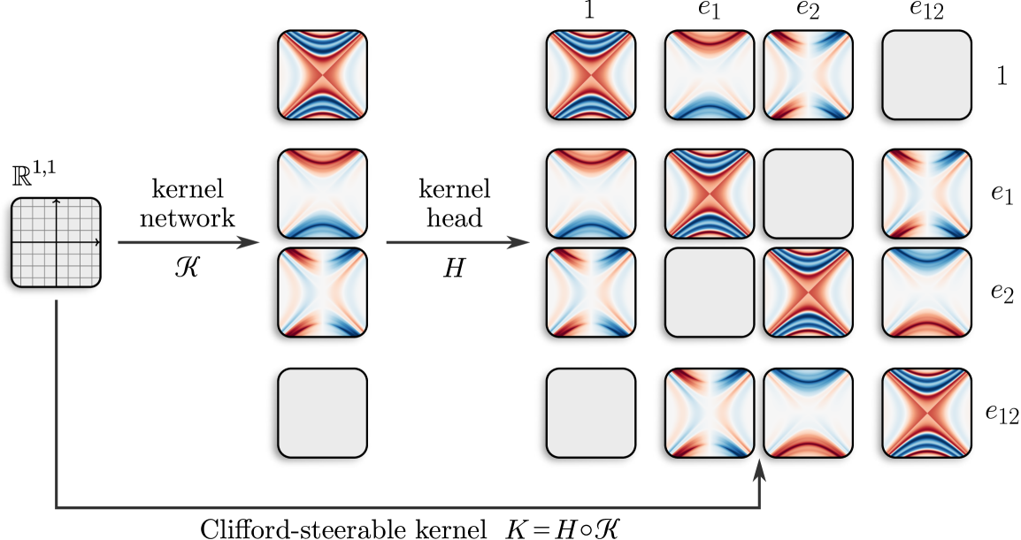
  Figure 4: Implicit Clifford-steerable kernel for ${(p,\mkern-2.0muq)\mkern-2.0mu=\mkern-2.0mu(1,\mkern-2.0mu1)}$ and ${c_{\mathrm{in}}}=$ ${{c_{\mathrm{out}}}\mkern-2.0mu=\mkern-2.0mu1}$. It is parameterized by a kernel network $\mathscr{K}$, producing a field of (${{c_{\mathrm{in}}}\mkern-4.0mu\times\mkern-4.0mu{c_{\mathrm{out}}}}$) multi-vector valued outputs. These are convolved with multivector fields by taking their (weighted) geometric product at each location in a convolutional manner. This is equivalent to a conventional steerable convolution after expansion to a ${\operatorname{O}(1,\mkern-3.0mu1)}$-steerable kernel via a kernel head operation $H$. For more details and equivariance properties see the commutative diagram in Fig. 5. A more detailed variant for $\mathbb{R}^{2,0}$ and $\operatorname{O}(2)$ is shown in Fig. 10.

  3 Clifford-Steerable CNNs

  This section presents Clifford-Steerable Convolutional Neural Networks (CS-CNNs), which operate on multivector fields on $\mathbb{R}^{p,q}$, and are equivariant to the isometry group $\operatorname{E}(p,q)$ of $\mathbb{R}^{p,q}$. To achieve $\operatorname{E}(p,q)$-equivariance, we need to find a way to implement $\operatorname{O}(p,q)$-steerable kernels (Section 2.2), which we do by leveraging the connection between $\operatorname{Cl}(\mathbb{R}^{p,q})$ and $\operatorname{O}(p,q)$ presented in Section 2.3.

  CS-CNNs process (multi-channel) multivector fields

  $$f:\mathbb{R}^{p,q}\to\operatorname{Cl}(\mathbb{R}^{p,q})^{c}$$ (28)

  of type $(W,\rho)=(\operatorname{Cl}(\mathbb{R}^{p,q})^{c},\rho_{\operatorname{Cl}}^{c})$ with $c\geq 1$ channels. The representation

  $$\rho_{\operatorname{Cl}}^{c}\,=\,{\textstyle\bigoplus\nolimits_{i=1}^{c}}\rho_{\operatorname{Cl}}:\ \operatorname{O}(p,q)\to\operatorname{GL}\!\big{(}\!\operatorname{Cl}(\mathbb{R}^{p,q})^{c}\big{)}$$ (29)

  is given by the action $\rho_{\operatorname{Cl}}$ from 2.14, however, applied to each of the $c$ components individually.

  Following 2.12, our main goal is the construction of a convolution operator

  $$L:\,\Gamma\big{(}\mathbb{R}^{p,q},\operatorname{Cl}(\mathbb{R}^{p,q})^{{c_{\mathrm{in}}}}\big{)}\to\Gamma\big{(}\mathbb{R}^{p,q},\operatorname{Cl}(\mathbb{R}^{p,q})^{{c_{\mathrm{out}}}}\big{)},$$

  $$L(f_{\textup{in}})(u):=\int_{\mathbb{R}^{p,q}}K(v)\big{[}f_{\textup{in}}(u-v)\big{]}\,dv,\mkern 10.0mu$$ (30)

  parameterized by a convolution kernel

  $$K:\,\mathbb{R}^{p,q}\to\operatorname{Hom}_{\mathrm{Vec}}\!\big{(}\!\operatorname{Cl}(\mathbb{R}^{p,q})^{c_{\mathrm{in}}},\operatorname{Cl}(\mathbb{R}^{p,q})^{c_{\mathrm{out}}}\big{)}$$ (31)

  that satisfies the following $\operatorname{O}(p,q)$-steerability (equivariance) constraint

  $$\mkern-6.0muK(gv)\,\stackrel{{\scriptstyle!}}{{=}}\,\rho_{\operatorname{Cl}}^{{c_{\mathrm{out}}}}(g)\,K(v)\,\rho_{\operatorname{Cl}}^{{c_{\mathrm{in}}}}(g^{\scalebox{0.75}[1.0]{$-$}1})\,=:\,\rho_{\operatorname{Hom}}(g)(K(v)),$$

  for every $g\in\operatorname{O}(p,q)$ and $v\in\mathbb{R}^{p,q}$.

  As mentioned in Section 2.2.2, constructing such $\operatorname{O}(p,q)$-steerable kernels is typically hard. To overcome this challenge, we follow Zhdanov et al. (2022) and implement the kernels implicitly. Specifically, they are based on $\operatorname{O}(p,q)$-equivariant “kernel networks”

  $$\mathscr{K}:\,\mathbb{R}^{p,q}\to\operatorname{Cl}(\mathbb{R}^{p,q})^{{c_{\mathrm{out}}}\times{c_{\mathrm{in}}}},$$ (33)

  implemented as CGENNs (Section 2.3.3).

  Unfortunately, the codomain of $\mathscr{K}$ is $\operatorname{Cl}(\mathbb{R}^{p,q})^{{c_{\mathrm{out}}}\times{c_{\mathrm{in}}}}$ instead of $\operatorname{Hom}_{\mathrm{Vec}}\!\big{(}\!\operatorname{Cl}(\mathbb{R}^{p,q})^{c_{\mathrm{in}}},\operatorname{Cl}(\mathbb{R}^{p,q})^{c_{\mathrm{out}}}\big{)}$, as required by steerable kernels (Eq. 31). To bridge the gap between these spaces, we introduce an $\operatorname{O}(p,q)$-equivariant linear layer, called kernel head $H$. Its purpose is to transform the kernel network’s output $\mathscr{k}:=\mathscr{K}(v)\in\operatorname{Cl}(\mathbb{R}^{p,q})^{{c_{\mathrm{out}}}\times{c_{\mathrm{in}}}}$ into the desired $\mathbb{R}$-linear map between multivector channels $H(\mathscr{k})\in\operatorname{Hom}_{\mathrm{Vec}}\!\big{(}\!\operatorname{Cl}(\mathbb{R}^{p,q})^{c_{\mathrm{in}}},\operatorname{Cl}(\mathbb{R}^{p,q})^{c_{\mathrm{out}}}\big{)}$. The relation between the kernel network $\mathscr{K}$, the kernel head $H$, and the resulting steerable kernel $K:=H\circ\mathscr{K}$ is visualized in Fig.  5 (right). Figs. 4 and 5.

  To achieve ${\operatorname{O}(p,\mkern-2.0muq)}$-equivariance (steerability) of ${K\mkern-3.5mu=\mkern-2.5muH\mkern-3.0mu\circ\mkern-2.0mu\mathscr{K}\mkern-2.5mu,}$ we have to make the kernel head $H$ of a specific form:

  Figure 5:   Construction and ${\operatorname{O}(p,\mkern-2.0muq)}$- equivariance of implicit steerable kernels ${K\mkern-3.0mu=\mkern-2.0muH\mkern-2.0mu\circ\mkern-2.0mu\mathscr{K}}$, which are composed from a kernel network $\mathscr{K}$ with ${{c_{\mathrm{out}}}\mkern-5.0mu\times\mkern-5.0mu{c_{\mathrm{in}}}}$ multivector outputs and a kernel head $H$. The whole diagram commutes. The two inner squares show the individual equivariance of $\mathscr{K}$ and $H$, from which the kernel’s overall equivariance follows.

  Definition 3.1 (Kernel head).

  A kernel head is a map

  $$H\mkern-4.0mu:\mkern 1.0mu\operatorname{Cl}(\mathbb{R}^{p,q})^{{c_{\mathrm{out}}}\mkern-1.0mu\times{c_{\mathrm{in}}}}\! \to\operatorname{Hom}_{\mathrm{Vec}}\mkern-4.0mu\big{(}\mkern-4.0mu\operatorname{Cl}(\mathbb{R}^{p,q})^{c_{\mathrm{in}}}\!,\operatorname{Cl}(\mathbb{R}^{p,q})^{c_{\mathrm{out}}}\mkern-1.0mu\big{)}$$

  $$\mathscr{k} \mapsto H(\mathscr{k}),$$ (34)

  where the $\mathbb{R}$-linear operator

  $$H(\mathscr{k}):\,\operatorname{Cl}(\mathbb{R}^{p,q})^{c_{\mathrm{in}}} \to\operatorname{Cl}(\mathbb{R}^{p,q})^{c_{\mathrm{out}}}, \mathfrak{f} \mapsto H(\mathscr{k})[\mkern 2.0mu\mathfrak{f}\mkern 2.0mu],$$

  is defined on each output channel $i\in[{c_{\mathrm{out}}}]$ and grade component $k=0,\dots,d$, by:

  $$\mkern-6.0muH(\mathscr{k})[\mkern 2.0mu\mathfrak{f}\mkern 2.0mu]_{i}^{(k)} :=\sum\nolimits_{\begin{subarray}{c}j\in[{c_{\mathrm{in}}}]\\ m,n=0,\dots,d\end{subarray}}w_{mn,ij}^{k}\mkern-1.0mu\cdot\mkern-2.0mu\left(\mathscr{k}_{ij}^{(m)}\mathbin{\ThisStyle{\vbox{\hbox{\scalebox{0.65}{$\SavedStyle\bullet$}}}}}\mkern 2.0mu\mathfrak{f}_{j}^{(n)}\right)^{\!(k)}\mkern 6.0mu$$

  $m,n=0,\dots,d$ label grades and ${j\in[{c_{\mathrm{in}}}]}$ input channels. The $w_{mn,ij}^{k}\in\mathbb{R}$ are parameters that allow for weighted mixing between grades and channels.

  Our implementation of the kernel head is discussed in Section A.5. Note that the kernel head $H$ can be seen as a linear combination of partially evaluated geometric product layers $P^{(k)}(\mathscr{k}_{ij},\cdot)$ from (LABEL:eq:geom-prod-layer), which mixes input channels to get the output channels. The specific form of the kernel head $H$ comes from the following, most important property:

  Proposition 3.2 (Equivariance of the kernel head).

  The kernel head $H$ is $\operatorname{O}(p,q)$-equivariant w.r.t. $\rho_{\operatorname{Cl}}^{{c_{\mathrm{out}}}\times{c_{\mathrm{in}}}}$ and $\rho_{\operatorname{Hom}}$, i.e. for $g\in\operatorname{O}(p,q)$ and $\mathscr{k}\in\operatorname{Cl}(\mathbb{R}^{p,q})^{{c_{\mathrm{out}}}\times{c_{\mathrm{in}}}}$ we have:

  $$H\big{(}\rho_{\operatorname{Cl}}^{{c_{\mathrm{out}}}\times{c_{\mathrm{in}}}}(g)(\mkern 2.0mu\mathscr{k})\big{)} \,=\,\rho_{\operatorname{Hom}}(g)(H(\mkern 2.0mu\mathscr{k})\mkern 2.0mu).$$ (36)

  Proof.

  The proof relies on the $\operatorname{O}(p,q)$-equivariance of the geometric product and of linear combinations within grades. It can be found in the Appendix in Appendix E. ∎

  With these obstructions out of the way, we can now give the core definition of this paper:

  Definition 3.3 (Clifford-steerable kernel).

  A Clifford-steerable kernel $K$ is a map as in Eq. (31) that factorizes as: $K=H\circ\mathscr{K}$ with a kernel head $H$ from Eq. (LABEL:eq:kernel-head-1) and a kernel network $\mathscr{K}$ given by a Clifford group equivariant neural network (CGENN) from 2.16:

  $$\mathscr{K}=[\mathscr{K}_{ij}]_{\begin{subarray}{c}i\in[{c_{\mathrm{out}}}]\\ j\in[{c_{\mathrm{in}}}]\end{subarray}}:\mathbb{R}^{p,q}\to\operatorname{Cl}(\mathbb{R}^{p,q})^{{c_{\mathrm{out}}}\times{c_{\mathrm{in}}}}.$$ (37)

  The main theoretical result of this paper is that Clifford-steerable kernels are always $\operatorname{O}(p,q)$-steerable:

  Theorem 3.4 (Equivariance of Clifford-steerable kernels).

  Every Clifford-steerable kernel ${K\mkern-2.0mu=\mkern-2.0muH\mkern-2.0mu\circ\mkern-2.0mu\mathscr{K}}$ is $\operatorname{O}(p,q)$-steerable w.r.t. the standard action ${\rho(g)\mkern-2.0mu=\mkern-1.5mug}$ and $\rho_{\operatorname{Hom}}$:

  $$K(gv)\,=\,\rho_{\operatorname{Hom}}(g)(K(v))\mkern 24.0mu\forall\ g\in\operatorname{O}(p,\mkern-1.5muq),\ v\in\mathbb{R}^{p,q}$$

  Proof.

  $\mathscr{K}$ and $H$ are $\operatorname{O}(p,q)$-equivariant by Definition/The-orem 2.16 and 3.2, respectively. The $\operatorname{O}(p,q)$-equivariance of the composition $K=H\circ\mathscr{K}$ then follows from Fig. 5 or by direct calculation:

  $$K(gv)\ =\ H\big{(}\mathscr{K}(gv)\big{)}$$ (38)

  $$=\ H\big{(}\rho_{\operatorname{Cl}}^{{c_{\mathrm{out}}}\times{c_{\mathrm{in}}}}(g)(\mathscr{K}(v))\big{)}$$

  $$=\ \rho_{\operatorname{Hom}}(g)\left(H\big{(}\mathscr{K}(v)\big{)}\right)$$

  $$=\ \rho_{\operatorname{Hom}}(g)\big{(}K(v)\big{)}.\qed$$

  A direct Corollary of 3.4 and 2.12 is now the following desired result.

  Corollary 3.5.

  ​Let ${K\mkern-3.0mu=\mkern-3.0muH\mkern-3.0mu\circ\mkern-2.5mu\mathscr{K}}$ be a Clifford-steerable kernel. The corresponding convolution operator $L$ (Eq. (3)) is then $\operatorname{E}(p,q)$-equivariant; for all $f_{\mathrm{in}}\in\operatorname{\Gamma}\big{(}\mathbb{R}^{p,q},\operatorname{Cl}(\mathbb{R}^{p,q})^{c_{\mathrm{in}}}\big{)}$:

  $$(t,g)\rhd L(f_{\mathrm{in}}) =L\big{(}(t,g)\rhd f_{\mathrm{in}}\big{)}\mkern 24.0mu\forall\,(t,\mkern-2.0mug)\in\operatorname{E}(p,q)$$

  Definition 3.6 (Clifford-steerable CNN).

  We call a convolutional network (that operates on multivector fields and is) based on Clifford-steerable kernels a Clifford-Steerable Convolutional Neural Network (CS-CNN).

  Remark 3.7.

  Brandstetter et al. (2023) use a similar kernel head $H$ as ours in Eq. (LABEL:eq:kernel-head-1). However, as their implicit kernel network $\mathscr{K}$ is not $\operatorname{O}(p,\mkern-1.0muq)$-equivariant, they only achieve translation equivariance, while our CS-CNNs are fully $\operatorname{E}(p,\mkern-1.0muq)$-equivariant.

  Appendix F generalizes CS-CNNs from flat spacetimes to general curved pseudo-Riemannian manifolds. Appendix A provides details on the code implementation of CS-CNNs, available at https://github.com/maxxxzdn/clifford-group-equivariant-cnns.

  4 Experimental Results

  

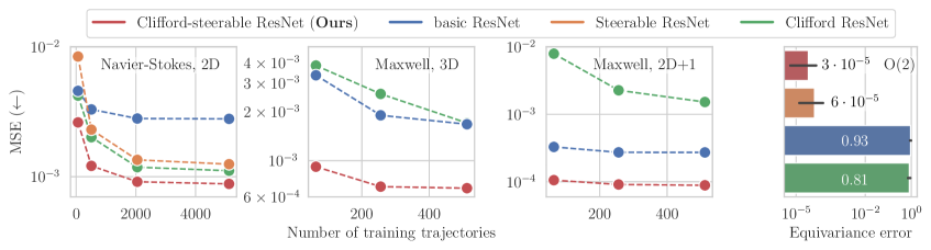
  Figure 6: Left: Mean squared errors (MSEs) on various PDE forecasting tasks (one-step loss). CS-ResNets significantly outperform all baselines regardless of the volume of training data. Right: Relative equivariance error for $\operatorname{O}(2)$, measuring how well the models commute with group actions. Note that the axis label is logarithmic.

  To assess CS-CNNs, we investigate how well they can learn to simulate dynamical systems by testing their ability to predict future states given a history of recent states (Gupta & Brandstetter, 2022). We consider three settings:

  • Fluid dynamics on $\mathbb{R}^{2}$ (incompressible Navier-Stokes);

  • Electrodynamics on $\mathbb{R}^{3}\mkern 12.0mu$ (Maxwell’s equations);

  • Electrodynamics on $\mathbb{R}^{1,2}$ (Maxwell’s equations).

  Only the last setting is properly incorporating time into ${1\mkern-4.0mu+\mkern-3.0mu2}$-dimensional spacetime, while the former two are treating time steps improperly as feature channels. The improper setting allows us to compare our method with prior work, which was not able to incorporate the full spacetime symmetries $\operatorname{E}(1,n)$, but only the spatial subgroup $\operatorname{E}(n)$ (which is also covered by CS-CNNs).

  

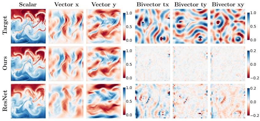
  Figure 7: Left: target and predicted fields on $\mathbb{R}^{2,0}$ for Navier-Stokes when rotated by $90^{\circ}$. CS-ResNet (ours) is trained on only $64$ trajectories, the basic ResNet on $5120$. Right: relative difference between target (upper row) and predicted fields on $\mathbb{R}^{1,2}$ for Maxwell 2D under arbitrary reflections.

  

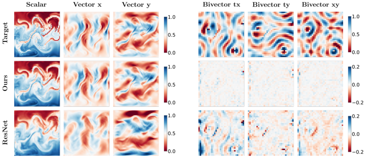
  Figure 8: Left: target and predicted fields on $\mathbb{R}^{(2,0)}$ for Navier-Stokes when rotated by $90^{\circ}$. CS-ResNet (ours) is trained on only $64$ trajectories, the basic ResNet on $5120$. Right: relative difference between target (upper row) and predicted fields on $\mathbb{R}^{(1,2)}$ for Maxwell 2D under arbitrary reflections.

  Data & Tasks: For fluid dynamics and electrodynamics forecasting on $\mathbb{R}^{2}\equiv\mathbb{R}^{2,0}$ and $\mathbb{R}^{3}\equiv\mathbb{R}^{3,0}$, respectively, the goal is to predict the next state given 4 previous time steps. The input consists of scalar pressure and vector velocity fields for the former, and vector electric and bivector magnetic fields for the latter. For electrodynamics on $\mathbb{R}^{1,2}$, the model is given 16 time steps in the past, and should predict 16 steps to the future. In this case, the entire electromagnetic field forms a bivector (Orbán & Mira, 2020). More details on the datasets are found in Appendix C.1.

  Architectures: We evaluate four architectures:

  • Clifford-Steerable ResNets (${\operatorname{E}(p,\mkern-2.0muq)}$-equivariant);

  • conventional ResNets (translation equivariant);

  • Clifford ResNets (translation equivariant);

  • Steerable ResNets ($\operatorname{E}(n)$-equivariant).

  The basic ResNet architecture is described in Appendix C. Clifford, Steerable, and our CS-ResNets are constructed by substituting conventional convolutions, respectively, with Clifford convolutions from (Brandstetter et al., 2023), $\operatorname{O}(n)$-steerable convolutions from (Weiler & Cesa, 2019; Cesa et al., 2022), and our Clifford-Steerable convolutions from Section 3. All models scale the number of channels to match the parameter count of the basic ResNet.

  Results: We evaluate the models on various training set sizes and report mean-squared error (MSE) losses. As shown in Fig. 6, our CS-ResNets outperform the baselines on all tasks and across all dataset sizes, with particularly high advantage on modeling Maxwell’s equations. Our CS-ResNets are extremely sample-efficient: In the Navier-Stokes experiment, they require only $64$ trajectories to outperform the basic ResNet trained on 80$\times$ more data.

  The Maxwell dataset on spacetime $\mathbb{R}^{1,2}$ is naturally described by the space-time algebra $\operatorname{Cl}(\mathbb{R}^{1,2})$ (Hestenes, 2015). Time appears here as a grid dimension, not as a channel, contrary to the previous experiments. The light cone structure of CS-CNN kernels (Fig. 5) ensures the models’ consistency across different inertial frames of reference.

  Equivariance error: Finally, we asses the models’ $\operatorname{E}(2)$-equivariance. We do this by measuring the relative error $\frac{\left|x-y\right|}{\left|x+y\right|}$ between (1) the output computed from a transformed input; and (2) the transformed output, given the original input. Quantitative results are reported in Fig. 6 (right), while Fig. 8 compares the output fields visually. As expected, the error for non-equivariant models is much larger than for the equivariant networks. The non-zero error of both $\operatorname{E}(2)$-equivariant models is due to numerical artefacts.

  5 Conclusions

  6 Conclusions

  We presented Clifford-Steerable CNNs, a new theoretical framework for ${\operatorname{E}(p,\mkern-1.5muq)}$-equivariant convolutions on pseudo-Euclidean spaces like Minkowski-spacetime. CS-CNNs process fields of multivectors – geometric features which naturally occur in many areas of physics. The required ${\operatorname{O}(p,\mkern-1.5muq)}$-steerable convolution kernels are implemented implicitly via Clifford group equivariant neural networks. This makes so far unknown analytic solutions for the steerability constraint unnecessary. CS-CNNs significantly outperform baselines on a variety of physical dynamics tasks.

  From the viewpoint of general steerable CNNs, there are some limitations:

  • First, there exist more general field types (${\operatorname{O}(p,\mkern-1.5muq)}$-rep-resentations) than multivectors, for which CS-CNNs do not provide steerable kernels. For connected Lie groups, like the subgroups ${\operatorname{SO}^{+}(p,\mkern-1.5muq)}$, these types can in principle be computed numerically (Shutty & Wierzynski, 2022).

  • Second, CGENNs and CS-CNNs rely on equivariant operations that treat multivector-grades $\operatorname{Cl}^{(k)}(V,\eta)$ as “atomic” features. However, it is not clear whether grades are always irreducible representations, that is, there might be further equivariant degrees of freedom which would treat irreducible sub-representations independently.

  • We observed that the steerable kernel spaces of CS-CNNs are not necessarily complete, that is, certain degrees of freedom might be missing. However, we show in Appendix B how they are recovered by composing multiple convolutions.

  • $\operatorname{O}(p,q)$ and their group orbits on $\mathbb{R}^{p,q}$ are for $p,q\neq 0$ non-compact; for instance, the hyperbolas in spacetimes $\mathbb{R}^{1,q}$ extend to infinity. In practice, we sample convolution kernels on a finite sized grid as shown in Fig. 5 (left). Fig. 4. This introduces a cutoff, breaking equivariance for large transformations. Note that this is an issue not specific to CS-CNNs, but it applies e.g. to scale-equivariant CNNs as well (Bekkers, 2020; Romero et al., 2020).

  Despite these limitations, CS-CNNs excel in our experiments.

  A major advantage of CGENNs and CS-CNNs is that they allow for a simple, unified implementation for arbitrary signatures ${(p,\mkern-2.0muq)}$. This is remarkable, since steerable kernels usually need to be derived for each symmetry group individually. Furthermore, our implementation applies both to multivector fields sampled on pixel grids and point clouds.

  CS-CNNs are, to the best of our knowledge, the first convolutional networks that respect the full symmetries ${\operatorname{E}(p,\mkern-1.5muq)}$ of Minkowski spacetime or any other pseudo-Euclidean spaces. Even more generally, CS-CNNs are readily extended to arbitrary curved pseudo-Riemannian manifolds, and such convolutions will necessarily rely on ${\operatorname{O}(p,\mkern-1.5muq)}$-steerable kernels. For more details see Appendix F and (Weiler et al., 2023). They could furthermore be adapted to steerable PDOs (partial differential operators) (Jenner & Weiler, 2022), which would connect them to the multivector calculus used in mathematical physics (Hestenes, 1968; Hitzer, 2002; Lasenby et al., 1993).

  Broader impact

  The broader implications of our work are primarily in the improved modeling of PDEs, other physical systems, or multi-vector based applications in computational geometry. Being able to model such systems more accurately can lead to better understanding about the physical systems governing our world, while being able to model such systems more efficiently could greatly improve the ecological footprint of training ML models for modeling physical systems.

  Acknowledgement

  This research was supported by Microsoft Research AI4Science. All content represents the opinion of the authors, which is not necessarily shared or endorsed by their respective employers/sponsors.

  Appendix

  Appendix A Implementation details

  This appendix provides details on the implementation of CS-CNNs.

  Before detailing the Clifford-steerable kernels and convolutions, we first define the following “kernel shell” operation, which is used twice in the final kernel computation. Recall that given the base space $\mathbb{R}^{p,q}$ equipped with the inner product $\eta^{p,q}$, we have a Clifford algebra $\operatorname{Cl}(\mathbb{R}^{p,q})$. We want to compute a kernel that maps from ${c_{\mathrm{in}}}$ multivector input channels to ${c_{\mathrm{out}}}$ multivector output channels, i.e.,

  $$K:\,\mathbb{R}^{p,q}\to\operatorname{Hom}_{\mathrm{Vec}}\!\big{(}\!\operatorname{Cl}(\mathbb{R}^{p,q})^{c_{\mathrm{in}}},\operatorname{Cl}(\mathbb{R}^{p,q})^{c_{\mathrm{out}}}\big{)}\,.$$ (39)

  $K$ is defined on any $v\in\mathbb{R}^{p,q}$, which allows to model point clouds. In this work, however, we sample it on a grid of shape $X_{1},\dots,X_{p+q}$, analogously to typical CNNs.

  A.1 Clifford Embedding

  We briefly discuss how one is able to embed scalars and vectors into the Clifford algebra. This extends to other grades such as bivectors.

  Let $s\in\mathbb{R}$ and $v\in\mathbb{R}^{p,q}$. Using the natural isomorphisms $\mathcal{E}^{(0)}:\mathbb{R}\xrightarrow{\sim}\operatorname{Cl}(\mathbb{R}^{p,q})^{(0)}$ and $\mathcal{E}^{(1)}:\mathbb{R}^{p,q}\xrightarrow{\sim}\operatorname{Cl}(\mathbb{R}^{p,q})^{(1)}$, we embed the scalar and vector components into a multivector as

  $$m\,:=\,\mathcal{E}^{(0)}(s)+\mathcal{E}^{(1)}(v)\ \ \in\ \operatorname{Cl}(\mathbb{R}^{p,q})\,.$$ (40)

  This is a standard operation in Clifford algebra computations, where we leave the other components of the multivector zero. We denote such embeddings in the algorithms provided below jointly as “$\textsc{cl\_embed}([s,v])$”.

  A.2 Scalar Orbital Parameterizations

  Note that the $\operatorname{O}(p,q)$-steerability constraint

  $$K(gv)\,\stackrel{{\scriptstyle!}}{{=}}\,\rho_{\operatorname{Cl}}^{{c_{\mathrm{out}}}}(g)\,K(v)\,\rho_{\operatorname{Cl}}^{{c_{\mathrm{in}}}}(g^{\scalebox{0.75}[1.0]{$-$}1})\,=:\,\rho_{\operatorname{Hom}}(g)(K(v))$$

  $$\forall\ v\in\mathbb{R}^{p,q},\ g\in\operatorname{O}(p,q)$$

  couples kernel values within but not across different $\operatorname{O}(p,q)$-orbits

  $$\operatorname{O}(p,q).v\,:= \,\ \{gv\,|\,g\in\operatorname{O}(p,q)\}$$ (41)

  $$= \,\ \{w\,|\,\eta(w,w)=\eta(v,v)\}\,.$$

  The first line here is the usual definition of group orbits, while the second line makes use of the Def. 2.5 of pseudo-orthogonal groups as metric-preserving linear maps.

  Function 1 ScalarShell

    input $\eta^{p,q}$, $v\in\mathbb{R}^{p,q}$, $\sigma$.

    $s\leftarrow\operatorname{sgn}\left(\eta^{p,q}(v,v)\right)\cdot\exp\left(-\frac{\left|\eta^{p,q}(v,v)\right|}{2\sigma^{2}}\right)$

    return  $s$

  Function 2 CliffordSteerableKernel

    input $p,q$ $\Lambda$, ${c_{\mathrm{in}}}$, ${c_{\mathrm{out}}}$, $\left(v_{n}\right)_{n=1}^{N}\in\mathbb{R}^{p,q}$, $\mathrm{CGENN}$

    output $\mathscr{k}\in\mathbb{R}^{({c_{\mathrm{out}}}\cdot 2^{d})\times({c_{\mathrm{in}}}\cdot 2^{d})\times X_{1}\times\dots\times X_{p+q}}$

    

    # Weighted Cayley.

    for $i=1\dots c_{\mathrm{in}}$, $o=1\dots c_{\mathrm{out}}$, $a,b,c=1\dots p+q$ do

       $w^{c}_{oiab}\sim\mathcal{N}(0,\frac{1}{\sqrt{{c_{\mathrm{in}}}\cdot N}})$ # Weight init.

       $W^{c}_{oiab}\leftarrow\Lambda_{ab}^{c}\cdot w^{c}_{oiab}$

    end for

    

    $\sigma\sim\mathcal{U}(0.4,0.6)$ # Init if needed.

    # Compute scalars.

    $s_{n}\leftarrow\textsc{ScalarShell}(\eta^{p,q},v_{n},\sigma)$

    # Embed $s$ and $v$ into a multivector.

    $x_{n}\leftarrow\textsc{cl\_embed}\left(\left[s_{n},v_{n}\right]\right)$

    

    # Evaluate kernel network.

    $\mathscr{k}_{n}^{io}:=\mathrm{CGENN}\left(x_{n}\right)$

    

    # Reshape to kernel matrix.

    $\mathscr{k}\leftarrow\textsc{reshape}\left(\mathscr{k},(N,{c_{\mathrm{out}}},{c_{\mathrm{in}}})\right)$

    

    # Compute kernel mask.

    for $i=1\dots c_{\mathrm{in}}$, $o=1\dots c_{\mathrm{out}}$, $k=0\dots p+q$ do

       $\sigma_{kio}\sim\mathcal{U}(0.4,0.6)$ # Init if needed.

       $s_{noi}^{{k}}\leftarrow\textsc{ScalarShell}(\eta^{p,q},v_{n},\sigma_{kio})$

    end for

    

    $\mathscr{k}_{noi}^{(k)}\leftarrow\mathscr{k}_{noi}^{(k)}\cdot s_{noi}^{k}$ # Mask kernel.

    

    # Kernel head.

    $\mathscr{k}_{noib}^{c}\leftarrow\sum_{a=1}^{2^{d}}\mathscr{k}_{noi}^{a}\cdot W^{c}_{oiab}$ # Partial weighted geometric product.

    

    # Reshape to final kernel.

    $\mathscr{k}\leftarrow\textsc{reshape}\left(\mathscr{k},\left({c_{\mathrm{out}}}\cdot 2^{d},{c_{\mathrm{in}}}\cdot 2^{d},X_{1},\dots,X_{p+q}\right)\right)$

    return  $\mathscr{k}$

  Function 3 CliffordSteerableConvolution

    input $F_{\mathrm{in}}$, $\left(v_{n}\right)_{n=1}^{N}$, Args

    output $F_{\mathrm{out}}$

    $F_{\mathrm{in}}\leftarrow$ reshape$(F_{\mathrm{in}},(B,{c_{\mathrm{in}}}\cdot 2^{d},Y_{1},\dots,Y_{p+q}))$

    $\mathscr{k}\leftarrow$ CliffordSteerableKernel$(\left(v_{n}\right)_{n=1}^{N},\textsc{Args})$

    $F_{\mathrm{out}}\leftarrow\textsc{Conv}(F_{\mathrm{in}},\mathscr{k})$

    $F_{\mathrm{out}}\leftarrow$ reshape$(F_{\mathrm{out}},(B,{c_{\mathrm{out}}},Y_{1},\dots,Y_{p+q},2^{d}))$

    return  $F_{\mathrm{out}}$

  In the positive-definite case of $\operatorname{O}(n)$, this means that the only degree of freedom is the radial distance from the origin, resulting in (hyper)spherical orbits. Examples of such kernels can be seen in Fig. 10. Other radial kernels are obtained typically through e.g. Gaussian shells, Bessel functions, etc.

  In the nondefinite case of $\operatorname{O}(p,q)$, the orbits are hyperboloids, resulting in hyperboloid shells for e.g. the Lorentz group $\operatorname{O}(1,3)$ as in Fig. 5 (left). Fig. 4. In this case, we extend the input to the kernel with a scalar component that now relates to the hyperbolic (squared) distance from the origin.

  Specifically, we define an exponentially decaying $\eta^{p,q}$-induced (parameterized) scalar orbital shell (analogous to the radial shell of typical Steerable CNNs) in the following way. We parameterize a kernel width $\sigma$ and compute the shell value as

  $$s_{\sigma}(v)=\operatorname{sgn}\left(\eta^{p,q}(v,v)\right)\cdot\exp\left(-\frac{\left|\eta^{p,q}(v,v)\right|}{2\sigma^{2}}\right).$$ (42)

  The width $\sigma\sim\mathcal{U}(0.4,0.6)$ is, inspired by (Cesa et al., 2022), initialized with a uniform distribution. Since $\eta^{p,q}(v,v)$ can be negative in the nondefinite case, we take the absolute value and multiply the result by the sign of $\eta^{p,q}(v,v)$. Computation of the kernel shell (ScalarShell) is outlined in Function 1. Intuitively, we obtain exponential decay for points far from the origin. However, the sign of the inner product ensures that we clearly disambiguate between “light-like” and “space-like” points. I.e., they are close in Euclidean distance but far in the $\eta^{p,q}$-induced distance. Note that this choice of parameterizing scalar parts of the kernel is not unique and can be experimented with.

  A.3 Kernel Network

  Recall from Section 3 that the kernel $K$ is parameterized by a kernel network, which is a map

  $$\mathscr{K}:\,\mathbb{R}^{p,q}\to\operatorname{Cl}(\mathbb{R}^{p,q})^{{c_{\mathrm{out}}}\times{c_{\mathrm{in}}}}$$ (43)

  implemented as an $\operatorname{O}(p,q)$-equivariant CGENN. It consists of (linearly weighted) geometric product layers followed by multivector activations.

  Let $\{v_{n}\}_{n=1}^{N}$ be a set of sampling points, where $N:=X_{1}\cdot\ldots\cdot X_{p+q}$. In the remainder, we leave iteration over $n$ implicit and assume that the operations are performed for each $n$. We obtain a sequence of scalars using the kernel shell

  $$s_{n} :=s_{\sigma}(v_{n})\,.$$ (44)

  The input to the kernel network is a batch of multivectors

  $$x_{n}:=\textsc{cl\_embed}([s_{n},v_{n}])\,.$$ (45)

  I.e., taking $s$ and $v$ together, they form the scalar and vector components of the CEGNN’s input multivector. We found including the scalar component crucial for the correct scaling of the kernel to the range of the grid.

  Let $i=1,\dots,{c_{\mathrm{in}}}$ and $o=1,\dots,{c_{\mathrm{out}}}$ be a sequence of input and output channels. We then have the kernel network output

  $$\mathscr{k}_{noi}\ :=\ \mathscr{K}(v_{n})_{oi}\ :=\ \mathrm{CGENN}(x_{n})_{oi}\,,$$ (46)

  where $\mathscr{k}_{noi}\in\operatorname{Cl}(\mathbb{R}^{p,q})$ is the output of the kernel network for the input multivector $x_{n}$ (embedded from the scalar $s_{n}$ and vector $v_{n}$). Once the output stack of multivectors is computed, we reshape it from shape $(N,{c_{\mathrm{out}}}\cdot{c_{\mathrm{in}}})$ to shape $(N,{c_{\mathrm{out}}},{c_{\mathrm{in}}})$, resulting in the kernel matrix

  $$\mathscr{k}\leftarrow\textsc{reshape}\left(\mathscr{k},(N,{c_{\mathrm{out}}},{c_{\mathrm{in}}})\right)\,,$$ (47)

  where now $\mathscr{k}\in\operatorname{Cl}(\mathbb{R}^{p,q})^{N\times{c_{\mathrm{out}}}\times{c_{\mathrm{in}}}}$. Note that $k_{n}\in\operatorname{Cl}(\mathbb{R}^{p,q})^{{c_{\mathrm{out}}}\times{c_{\mathrm{in}}}}$ is a matrix of multivectors, as desired.

  A.4 Masking

  We compute a second set of scalars which will act as a mask for the kernel. This is inspired by Steerable CNNs to ensure that the (e.g., radial) orbits of compact groups are fully represented in the kernel, as shown in Figure 10. However, note that for $\operatorname{O}(p,q)$-steerable kernels with both $p,q\neq 0$ this is never fully possible since $\operatorname{O}(p,q)$ is in general not compact, and all orbits except for the origin extend to infinity. This can e.g. be seen in the hyperbolic-shaped kernels in Figure 5.

  For equivariance to hold in practice, whole orbits would need to be present in the kernel, which is not possible if the kernel is sampled on a grid with finite support. This is not specific to our architecture, but is a consequence of the orbits’ non-compactness. The same issue arises e.g. in scale-equivariant CNNs (Romero et al., 2020; Worrall & Welling, 2019; Ghosh & Gupta, 2019; Sosnovik et al., 2020; Bekkers, 2020; Zhu et al., 2019; Marcos et al., 2018; Zhang & Williams, 2022). Further experimenting is needed to understand the impact of truncating the kernel on the final performance of the model.

  We invoke the kernel shell function again to compute a mask for each $k=0,\dots,{p+q}$, $i=1,\dots,{c_{\mathrm{in}}}$, $o=1,\dots,{c_{\mathrm{out}}}$. That is, we have a weight array $\sigma_{kio}$, initialized identically as earlier, which is reused for each position in the grid.

  $$s^{k}_{nio} :=s_{\sigma_{kio}}(v_{n})\,.$$ (48)

  We then mask the kernel by scalar multiplication with the shell, i.e.,

  $$\mathscr{k}_{kio}^{(k)}\leftarrow\mathscr{k}_{nio}^{(k)}\cdot s_{nio}^{k}\,.$$ (49)

  A.5 Kernel Head

  Finally, the kernel head turns the “multivector matrices” into a kernel that can be used by, for example, torch.nn.ConvNd or jax.lax.conv. This is done by a partial evaluation of a (weighted) geometric product. Let $\mu,\nu\in\operatorname{Cl}(\mathbb{R}^{p,q})$ be two multivectors. Recall that $\dim\operatorname{Cl}(\mathbb{R}^{p,q})=2^{p+q}=2^{d}$.

  $$(\mu\mathbin{\ThisStyle{\vbox{\hbox{\scalebox{0.5}{$\SavedStyle\bullet$}}}}}\nu)^{C}=\sum\nolimits_{A}\sum\nolimits_{B}\mu^{A}\cdot\nu^{B}\cdot\Lambda^{C}_{AB}\,,$$ (50)

  where $A,B,C\subseteq[d]$ are multi-indices running over the $2^{d}$ basis elements of $\operatorname{Cl}(\mathbb{R}^{p,q})$. Here, $\Lambda\in\mathbb{R}^{2^{d}\times 2^{d}\times 2^{d}}$ is the Clifford multiplication table of $\operatorname{Cl}(\mathbb{R}^{p,q})$, also sometimes called a Cayley table. It is defined as

  $$\Lambda_{A,B}^{C}=\begin{cases}0&\text{if }A\triangle B\neq C\\ \operatorname{sgn}^{A,B}\cdot\bar{\eta}(e_{A\cap B},e_{A\cap B})&\text{if }A\triangle B=C\end{cases}\,.$$ (51)

  Here, $\triangle$ denotes the symmetric difference of sets, i.e., $A\triangle B=(A\setminus B)\cup(B\setminus A)$. Further,

  $$\operatorname{sgn}^{A,B}:=(-1)^{n_{A,B}},$$ (52)

  where $n_{A,B}$ is the number of adjacent “swaps” one needs to fully sort the tuple $(i_{1},\dots,i_{s},j_{1},\dots,j_{t})$, where $A=\{i_{1},\dots,i_{s}\}$ and $B=\{j_{1},\dots,j_{t}\}$. In the following, we identify the multi-indices $A$, $B$, and $C$ with a relabeling $a$, $b$, and $c$ that run from $1$ to $2^{d}$.

  Altogether, $\Lambda$ defines a multivector-valued bilinear form which represents the geometric product relative to the chosen multivector basis. We can weight its entries with parameters $w_{oiab}^{c}\in\mathbb{R}$, initialized as $w_{oiab}^{c}\sim\mathcal{N}(0,\frac{1}{\sqrt{{c_{\mathrm{in}}}\cdot N}})$. These weightings can be redone for each input channel and output channel, as such we have a weighted Cayley table $W\in\mathbb{R}^{2^{d}\times 2^{d}\times 2^{d}\times{c_{\mathrm{in}}}\times{c_{\mathrm{out}}}}$ with entries

  $$W^{c}_{oiab}\ :=\ \Lambda^{c}_{ab}w^{c}_{oiab}\,.$$ (53)

  Given the kernel matrix $\mathscr{k}$, we compute the kernel by partial (weighted) geometric product evaluation, i.e.,

  $$\mathscr{k}_{noib}^{c}\leftarrow\sum\nolimits_{a=1}^{2^{d}}\mathscr{k}_{noi}^{a}\cdot W^{c}_{oiab}\,.$$ (54)

  Finally, we reshape and permute $\mathscr{k}_{noib}^{c}$ from shape $(N,{c_{\mathrm{out}}},{c_{\mathrm{in}}},2^{d},2^{d})$ to its final shape, i.e.,

  $$\mathscr{k}\leftarrow\textsc{reshape}\left(\mathscr{k},\left({c_{\mathrm{out}}}\cdot 2^{d},{c_{\mathrm{in}}}\cdot 2^{d},X_{1},\dots,X_{p+q}\right)\right)\,.$$

  This is the final kernel that can be used in a convolutional layer, and can be interpreted (at each sample coordinate) as an element of $\operatorname{Hom}_{\mathrm{Vec}}\!\big{(}\!\operatorname{Cl}(\mathbb{R}^{p,q})^{c_{\mathrm{in}}},\operatorname{Cl}(\mathbb{R}^{p,q})^{c_{\mathrm{out}}}\big{)}$. The pseudocode for the Clifford-steerable kernel (CliffordSteerableKernel) is given in Function 2.

  A.6 Clifford-steerable convolution:

  As defined in Section 3, Clifford-steerable convolutions can be efficiently implemented with conventional convolutional machinery such as torch.nn.ConvNd or jax.lax.conv (see Function 3 (CliffordSteerableConvolution) for pseudocode). We now have a kernel $\mathscr{k}\in\mathbb{R}^{({c_{\mathrm{out}}}\cdot 2^{d})\times({c_{\mathrm{in}}}\cdot 2^{d})\times X_{1}\times\dots\times X_{p+q}}$ that can be used in a convolutional layer. Given batch size $B$, we now reshape the input stack of multivector fields $(B,{c_{\mathrm{in}}},Y_{1},\dots,Y_{p+q},2^{d})$ into $(B,{c_{\mathrm{in}}}\cdot 2^{d},Y_{1},\dots,Y_{p+q})$. The output array of shape $(B,{c_{\mathrm{out}}}\cdot 2^{d},Y_{1},\dots,Y_{p+q})$ is obtained by convolving the input with the kernel, which is then reshaped to $(B,{c_{\mathrm{out}}},Y_{1},\dots,Y_{p+q},2^{d})$, which can then be interpreted as a stack of multivector fields again.

  Appendix B Completeness of kernel spaces

  In order to not over-constrain the model, it is essential to parameterize a complete basis of ${\operatorname{O}(p,\mkern-2.0muq)}$-steerable kernels. Comparing our implicit ${\operatorname{O}(2,\mkern-2.0mu0)\mkern-1.0mu=\mkern-1.0mu\operatorname{O}(2)}$-steerable kernels with the analytical solution by (Weiler & Cesa, 2019), we find that certain degrees of freedom are missing; see Fig. 10.

  However, while these degrees of freedom are missing in a single convolution operation, they can always be recovered by applying two consecutively convolutions. This suggests that the overall expressiveness of CS-CNNs is (at least for $\operatorname{O}(2)$) not diminished. Moreover, two convolutions with kernels $\widehat{K}$ and $K$ can always be expressed as a single convolution with a composed kernel ${\widehat{K}\mkern-3.0mu*\mkern-3.0muK}$. As visualized below, this composed kernel recovers the full degrees of freedom reported in (Weiler & Cesa, 2019):

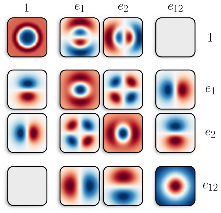
  Figure 9:

  

  The following two sections discuss the initial differences in kernel parametrizations and how they are resolved by adding a second linear or convolution operation. Unless stated otherwise, we focus here on ${c_{\mathrm{in}}}={c_{\mathrm{out}}}=1$ channels to reduce clutter.

  

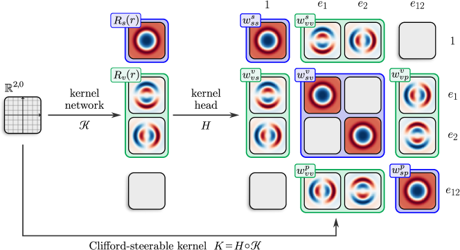
  foo CS-CNN parametrization scalar vector pseudoscalar $1$ $\phantom{\!\bigg{|}^{\top}}\big{[}e_{1},e_{2}\big{]}^{\top}$ $e_{12}$ $1$ $w^{s}_{ss}{\color[rgb]{0,0,1}R_{s}(r)}\,\big{[}\mkern 2.0mu1\mkern 2.0mu\big{]}$ $w^{s}_{vv}{\color[rgb]{0,1,0}R_{v}(r)}\,\big{[}\scalebox{0.75}[1.0]{$-$}\sin(\phi)\,\cos(\phi)\big{]}$ $\varnothing$ $\begin{bmatrix}e_{1}\\ e_{2}\end{bmatrix}$ $w^{v}_{vs}{\color[rgb]{0,1,0}R_{v}(r)}\,\begin{bmatrix}\scalebox{0.75}[1.0]{$-$}\!\sin(\phi)\\ \phantom{\scalebox{0.75}[1.0]{$-$}}\!\cos(\phi)\end{bmatrix}$                    $w^{v}_{sv}{\color[rgb]{0,0,1}R_{s}(r)}\,\begin{bmatrix}\;1&0~{}\\ \;0&1~{}\end{bmatrix}$ $w^{v}_{vp}{\color[rgb]{0,1,0}R_{v}(r)}\,\begin{bmatrix}\cos(\phi)\\ \sin(\phi)\\ \end{bmatrix}$ $e_{12}$ $\varnothing$ $w^{p}_{vv}{\color[rgb]{0,1,0}R_{v}(r)}\,\big{[}\cos(\phi)\,\phantom{-}\sin(\phi)\big{]}$ $w^{p}_{sp}{\color[rgb]{0,0,1}R_{s}(r)}\,\big{[}\mkern 2.0mu1\mkern 2.0mu\big{]}$ foo complete e2cnn parametrization (Weiler & Cesa, 2019) $1$ $\big{[}e_{1},e_{2}\big{]}^{\top}$ $e_{12}$ $1$ $R^{s}_{\ s}(r)\,\big{[}\mkern 2.0mu1\mkern 2.0mu\big{]}$ $R^{s}_{\ v}(r)\,\big{[}\scalebox{0.75}[1.0]{$-$}\sin(\phi)\,\cos(\phi)\big{]}$ $\varnothing$ $\begin{bmatrix}e_{1}\\ e_{2}\end{bmatrix}$   $R^{v}_{\ s}(r)\,\begin{bmatrix}\scalebox{0.75}[1.0]{$-$}\!\sin(\phi)\\ \phantom{\scalebox{0.75}[1.0]{$-$}}\!\cos(\phi)\end{bmatrix}$ $R^{v}_{\ v}(r)\mkern-3.0mu\begin{bmatrix}\;1&0~{}\\ \;0&1~{}\end{bmatrix}$ ,   $\widehat{R}^{v}_{\ v}(r)\mkern-3.0mu\begin{bmatrix}\cos(2\phi)\mkern-8.0mu&\phantom{\scalebox{0.75}[1.0]{$-$}}\sin(2\phi)\\ \sin(2\phi)\mkern-8.0mu&\scalebox{0.75}[1.0]{$-$}\cos(2\phi)\\ \end{bmatrix}$   $R^{v}_{\ p}(r)\,\begin{bmatrix}\cos(\phi)\\ \sin(\phi)\\ \end{bmatrix}$   $e_{12}$ $\varnothing$ $R^{p}_{\ v}(r)\,\big{[}\cos(\phi)\,\phantom{-}\sin(\phi)\big{]}$ $R^{p}_{\ p}(r)\,\big{[}\mkern 2.0mu1\mkern 2.0mu\big{]}$

  Figure 10: Comparison of the parametrization of $\operatorname{O}(2)$-steerable kernels in CS-CNNs (top and middle) and e2cnn (bottom). While the e2cnn solutions are proven to be complete, CS-CNN seems to miss certain degrees of freedom:
  (1) Their radial parts are coupled in the components highlighted in blue and green, while escnn allows for independent radial parts. By “coupled” we mean that they are merely scaled relative to each other with weights $w^{k}_{mn}$ from the weighted geometric product operation in the kernel head $H$, where $m$ labels grade $\mathscr{K}^{(m)}$ of the kernel network output while $n,k$ label input and output grades of the expanded kernel in $\operatorname{Hom}_{\mathrm{Vec}}\!\big{(}\mkern-2.0mu\operatorname{Cl}(\mathbb{R}^{p,q}),\,\operatorname{Cl}(\mathbb{R}^{p,q})\big{)}$;
  (2) CS-CNN is missing kernels of angular frequency $2$ that are admissible for mapping between vector fields; highlighted in red.
  As explained in Appendix B, these missing degrees of freedom are recovered when composing two convolution layers. A kernel corresponding to the composition of two convolutions in a single one is visualized in Fig. 9.

  B.1 Coupled radial dependencies in CS-CNN kernels

  The first issue is that the CS-CNN parametrization implies a coupling of radial degrees of freedom. To make this precise, note that the $\operatorname{O}(2)$-steerability constraint

  $$K(gv)\,\stackrel{{\scriptstyle!}}{{=}}\,\rho_{\operatorname{Cl}}^{{c_{\mathrm{out}}}}(g)\,K(v)\,\rho_{\operatorname{Cl}}^{{c_{\mathrm{in}}}}(g^{\scalebox{0.75}[1.0]{$-$}1})\quad\forall\ v\in\mathbb{R}^{2},\,g\in\operatorname{O}(2)$$

  decouples into independent constraints on individual $\operatorname{O}(2)$-orbits on $\mathbb{R}^{2}$, which are rings at different radii (and the origin); visualized in Fig. 2 (left). (Weiler et al., 2018a; Weiler & Cesa, 2019) parameterize the kernel therefore in (hyper)spherical coordinates. In our case these are polar coordinates of $\mathbb{R}^{2}$, i.e. a radius $r\in\mathbb{R}_{\geq 0}$ and angle $\phi\in S^{1}$:

  $$K(r,\phi)\,:=\,R(r)\kappa(\phi)$$ (55)

  The $\operatorname{O}(2)$-steerability constraint affects only the angular part and leaves the radial part entirely free, such that it can be parameterized in an arbitrary basis or via an MLP.

  e2cnn:

  Weiler & Cesa (2019) solved analytically for complete bases of the angular parts. Specifically, they derive solutions

  $$K^{k}_{\ n}(r,\phi)\,=\,R^{k}_{\ n}(r)\kappa^{k}_{\ n}(\phi)$$ (56)

  for any pair of input and output field types (irreps of grades) $n$ and $k$, respectively. This complete basis of $\operatorname{O}(2)$-steerable kernels is shown in the bottom table of Fig. 10.

  CS-CNNs:

  CS-CNNs parameterize the kernel in terms of a kernel network $\mathscr{K}:\mathbb{R}^{p,q}\to\operatorname{Cl}(\mathbb{R}^{p,q})^{{c_{\mathrm{out}}}\times{c_{\mathrm{in}}}}$, visualized in Fig. 10 (top). Expressed in polar coordinates, assuming ${c_{\mathrm{in}}}={c_{\mathrm{out}}}=1$, and considering the independence of $\mathscr{K}$ on different orbits due to its $\operatorname{O}(2)$-equivariance, we get the factorization

  $$\mathscr{K}(r,\phi)^{(m)}\ =\ R_{m}(r)\kappa_{m}(\phi)\,,$$ (57)

  where $m$ is the grade of the multivector-valued output. As described in Appendix A.5 (Eq. (53)), the kernel head operation $H$ expands this output by multiplying it with weights $W^{k}_{mn}=\Lambda^{k}_{mn}w^{k}_{mn}$, where $w^{k}_{mn}\in\mathbb{R}$ are parameters and $\Lambda^{k}_{mn}\in\{\scalebox{0.75}[1.0]{$-$}1,0,1\}$ represents the geometric product relative to the standard basis of $\mathbb{R}^{p,q}$. Note that we do not consider multiple in or output channels here. The final expanded kernel for CS-CNNs is hence given by

  $$K^{k}_{\ n}(r,\phi)\ =\ \sum_{m}W^{k}_{mn}\mathscr{K}(r,\phi)^{(m)}$$ (58)

  $$=\ \sum_{m}\Lambda^{k}_{mn}w^{k}_{mn}R_{m}(r)\kappa_{m}(\phi)\,.$$

  These solutions are listed in the top table in Fig. 10, and visualized in the graphics above.

  Comparison:

  Note that the complete solutions by (Weiler & Cesa, 2019) allow for a different radial part $R^{k}_{\ n}$ for each pair of input and output type (grade/irrep). In contrast, the CS-CNN parametrization expands coupled radial parts $R_{m}$, additionally multiplying them with weights $w^{k}_{mn}$ (highlighted in the table in blue and green). The CS-CNN parametrization is therefore clearly less general (incomplete).

  Solutions:

  One idea to resolve this shortcoming is to make the weighted geometric product parameters themselves radially dependent,

  $$w_{mn}^{k}:\ \mathbb{R}_{\geq 0}\to\mathbb{R},\quad r\mapsto w_{mn}^{k}(r)\,,$$ (59)

  for instance by parameterizing the weights with a neural network. This would fully resolve the under-parametrization, and would preserve equivariance, since $\operatorname{O}(2)$-steerability depends only on the angular variable.

  However, doing this is actually not necessary, since the missing flexibility of radial parts can always be resolved by running a convolution followed by a linear layer (or a second convolution) when ${c_{\mathrm{out}}}>1$. The reason for this is that different channels $i=1,\dots,{c_{\mathrm{out}}}$ of a kernel network $\mathscr{K}:\mathbb{R}\to\operatorname{Cl}(\mathbb{R})^{{c_{\mathrm{out}}}\times{c_{\mathrm{in}}}}$ do have independent radial parts. Their convolution responses in different channels can by a subsequent linear layer be mixed with grade-dependent weights. By linearity, this is equivalent to immediately mixing the channels’ radial parts with grade-dependent weights, resulting in effectively decoupled radial parts.

  B.2 Circular harmonics order 2 kernels

  A second issue is that the CS-CNN parametrization is missing a basis kernel of angular frequency $2$ that maps between vector fields; highlighted in red in the bottom table of Fig. 10. However, it turns out that this degree of freedom is reproduced as the difference of two consecutive convolutions ($*$), one mapping vectors to pseudoscalars and back to vectors, the other one mapping vectors to scalars and back to vectors, as suggested in the (non-commutative!) computation flow diagram below:

  As background on the angular frequency $2$ kernel, note that $\operatorname{O}(2)$-steerable kernels between irreducible field types of angular frequencies $j$ and $l$ contain angular frequencies $|j-l|$ and $j+l$ – this is a consequence of the Clebsch-Gordan decomposition of $\operatorname{O}(2)$-irrep tensor products (Lang & Weiler, 2020). We identify multivector grades $\operatorname{Cl}(\mathbb{R}^{2,0})^{(k)}$ with the following $\operatorname{O}(2)$-irreps:

  $$\textup{scalars}\in\operatorname{Cl}(\mathbb{R}^{2,0})^{(0)}\ \leftrightarrow\,\ \textup{trivial irrep (${j\!=\!0}$)}$$

  $$\textup{vectors}\in\operatorname{Cl}(\mathbb{R}^{2,0})^{(1)}\ \leftrightarrow\,\ \textup{defining irrep (${j\!=\!1}$)}$$

  $$\textup{pseudo-scalars}\in\operatorname{Cl}(\mathbb{R}^{2,0})^{(2)}\ \leftrightarrow\,\ \textup{sign-flip irrep (${j\!=\!0}$)}$$

  Kernels that map vector fields (${j\!=\!1}$) to vector fields (${l\!=\!1}$) should hence contain angular frequencies ${|j\mkern-2.0mu-\mkern-2.0mul|=0}$ and ${j\mkern-2.0mu+\mkern-2.0mul=2}$. The latter is missing since $\operatorname{O}(2)$-irreps of order $2$ are not represented by any grade of $\operatorname{Cl}(\mathbb{R}^{2,0})$.

  To solve this issue, it seems like one would have to replace the CEGNNs underlying the kernel network $\mathscr{K}$ with a more general $\operatorname{O}(2)$-equivariant MLP, e.g. (Finzi et al., 2021). However, it can as well be implemented as a succession of two convolution operations. To make this claim plausible, observe first that convolutions are associative, that is, two consecutive convolutions with kernels $K$ and $\widehat{K}$ are equivalent to a single convolution with kernel $\widehat{K}\ast K$:

  $$\widehat{K}\ast\big{(}K\ast f\big{)}\ =\ \big{(}\widehat{K}\ast K\big{)}\ast f$$ (60)

  Secondly, convolutions are linear, such that

  $$\alpha(\widehat{K}*f)+\beta(K*f)\ =\ \big{(}\alpha\widehat{K}+\beta K\big{)}\ast f$$ (61)

  for any $\alpha,\beta\in\mathbb{R}$.

  Using associativity, we can express two consecutive convolutions, first going from vector to scalar fields via

  $$K^{s}_{\ v}(r,\phi)\ =\ R^{s}_{\ v}(r)\begin{pmatrix}\scalebox{0.75}[1.0]{$-$}\sin(\phi)&\mkern-3.0mu\cos(\phi)\end{pmatrix}$$ (62)

  then going back from scalars to vectors via

  $$K^{v}_{\ s}(r,\phi)\ =\ R^{v}_{\ s}(r)\begin{pmatrix}\scalebox{0.75}[1.0]{$-$}\sin(\phi)\\[1.0pt] \phantom{\scalebox{0.75}[1.0]{$-$}}\cos(\phi)\end{pmatrix}$$ (63)

  as a single convolution between vector fields, where the combined kernel is given by:

  $$\Sigma^{v}_{\ v}\,:=\,K^{v}_{\ s}\ast K^{s}_{\ v}$$ (64)

  $$\ =\ \begin{pmatrix}\leavevmode\hbox to37.02pt{\vbox to37.02pt{\text{[drawing]}}}\\ \leavevmode\hbox to37.02pt{\vbox to37.02pt{\text{[drawing]}}}\end{pmatrix}\mkern-3.0mu\ast\mkern-3.0mu\begin{pmatrix}\leavevmode\hbox to37.02pt{\vbox to37.02pt{\text{[drawing]}}}&\mkern-8.0mu\leavevmode\hbox to37.02pt{\vbox to37.02pt{\text{[drawing]}}}\end{pmatrix}=\begin{pmatrix}\leavevmode\hbox to29.07pt{\vbox to29.07pt{\text{[drawing]}}}&\mkern-8.0mu\leavevmode\hbox to29.07pt{\vbox to29.07pt{\text{[drawing]}}}\\ \leavevmode\hbox to29.07pt{\vbox to29.07pt{\text{[drawing]}}}&\mkern-8.0mu\leavevmode\hbox to29.07pt{\vbox to29.07pt{\text{[drawing]}}}\end{pmatrix}$$

  We can similar define a convolution going from vector to pseudoscalar fields via

  $$K^{p}_{\ v}(r,\phi)\ =\ R^{p}_{\ v}(r)\begin{pmatrix}\cos(\phi)&\mkern-3.0mu\sin(\phi)\end{pmatrix}$$ (65)

  and back to vector fields via

  $$K^{v}_{\ p}(r,\phi)\ =\ R^{v}_{\ p}(r)\begin{pmatrix}\cos(\phi)\\[1.0pt] \sin(\phi)\end{pmatrix}$$ (66)

  as a single convolution with combined kernel:

  $$\Pi^{v}_{\ v}\,:=\,K^{p}_{\ v}\ast K^{v}_{\ p}$$ (67)

  $$\ =\ \begin{pmatrix}\leavevmode\hbox to37.02pt{\vbox to37.02pt{\text{[drawing]}}}\\ \leavevmode\hbox to37.02pt{\vbox to37.02pt{\text{[drawing]}}}\end{pmatrix}\mkern-3.0mu\ast\mkern-3.0mu\begin{pmatrix}\leavevmode\hbox to37.02pt{\vbox to37.02pt{\text{[drawing]}}}&\mkern-8.0mu\leavevmode\hbox to37.02pt{\vbox to37.02pt{\text{[drawing]}}}\end{pmatrix}=\begin{pmatrix}\leavevmode\hbox to29.07pt{\vbox to29.07pt{\text{[drawing]}}}&\mkern-8.0mu\leavevmode\hbox to29.07pt{\vbox to29.07pt{\text{[drawing]}}}\\ \leavevmode\hbox to29.07pt{\vbox to29.07pt{\text{[drawing]}}}&\mkern-8.0mu\leavevmode\hbox to29.07pt{\vbox to29.07pt{\text{[drawing]}}}\end{pmatrix}$$

  By linearity, we can define yet another convolution between vector fields by taking the difference of these kernels, which results in:

  $$\Pi^{v}_{\ v}-\Sigma^{v}_{\ v}\ =\ \begin{pmatrix}\leavevmode\hbox to32.68pt{\vbox to32.68pt{\text{[drawing]}}}&\leavevmode\hbox to32.68pt{\vbox to32.68pt{\text{[drawing]}}}\\ \leavevmode\hbox to32.68pt{\vbox to32.68pt{\text{[drawing]}}}&\leavevmode\hbox to32.68pt{\vbox to32.68pt{\text{[drawing]}}}\end{pmatrix}$$ (68)

  Such kernels parameterize exactly the missing $\operatorname{O}(2)$-steerable kernels of angular frequency $2$; highlighted in red in the bottom table in Fig. 10. This shows that the missing kernels can be recovered by two convolutions, if required.

  The “visual proof” by convolving kernels is clearly only suggestive. To make it precise, it would be required to compute the convolutions of two kernels analytically. This is easily done by identifying circular harmonics with derivatives of Gaussian kernels; a relation that is well known in classical computer vision (Lindeberg, 2009).

  Appendix C Experimental details

  Model details: For ResNets, we follow the setup of Wang et al. (2020); Brandstetter et al. (2023); Gupta & Brandstetter (2022): the ResNet baselines consist of 8 residual blocks, each comprising two convolution layers with $7\times 7$ (or $7\times 7\times 7$ for 3D) kernels, shortcut connections, group normalization (Wu & He, 2018), and GeLU activation functions (Hendrycks & Gimpel, 2016). We use two embedding and two output layers, i.e., the overall architectures could be classified as Res-20 networks. Following (Gupta & Brandstetter, 2022; Brandstetter et al., 2023), we abstain from employing down-projection techniques and instead maintain a consistent spatial resolution throughout the networks. The best models have approx. 7M parameters for Navier-Stokes and 1.5M parameters for Maxwell’s equations, in both 2D and 3D.

  Optimization: For each experiment and each model, we tuned the learning rate to find the optimal value. Each model was trained until convergence. For optimization, we used Adam optimizer (Kingma & Ba, 2014) with no learning decay and cosine learning rate scheduler (Loshchilov & Hutter, 2017) to reduce the initial value by the factor of 0.01. Training was done on a single node with 4 NVIDIA GeForce RTX 2080 Ti GPUs.

  C.1 Datasets

  We obtain the Navier-Stokes data from Gupta & Brandstetter (2022), based on $\Phi$Flow (Holl et al., 2020), on a grid with spatial resolution 128 x 128 ($\Delta x$ = 0.25, $\Delta y$ = 0.25), and temporal resolution of $\Delta t$ = 1.5 s. For validation and testing, we randomly selected 1024 trajectories from corresponding partitions. We obtain the 3D Maxwell’s equations from Brandstetter et al. (2023) on a grid with spatial resolution of $32\times 32\times 32(\Delta x=\Delta y=\Delta z=5\cdot 10^{-7})$, and temporal resolution of $\Delta t=50$s. In $\operatorname{Cl}(\mathbb{R}^{3,0})$, $\mathbf{E}$ is a vector, and $\mathbf{B}$ is a bivector. The size of validation and test partitions is 128. We generate the data for the 2D Maxwell’s equations using finite-difference time-domain (FDTD) (Taflove et al., 2005) simulations. We perform simulations on a closed domain with periodic boundary conditions on a grid with a spatial resolution of $128\times 128$ ($\Delta x=\Delta y=2\cdot 10\,\mathrm{m}^{-7}$), and temporal resolution of $\Delta t=65$ $\mu$s. We randomly place 4 different light sources outside a box, emitting light with different amplitude and phase shifts, causing the resulting $\mathbf{E}$ and $\mathbf{B}$ fields to interfere with each other. We confirm energy is conserved and downsample the resulting simulations to a spatial resolution of $32\times 32$ ($\Delta x=\Delta y=8\cdot 10\,\mathrm{m}^{-7}$). In $\operatorname{Cl}(\mathbb{R}^{1,2})$, the electromagnetic field forms a bivector (Orbán & Mira, 2020). The size of validation as well as test partitions was 128.

  Appendix D The Clifford Algebra

  For completeness purposes and to complement Section 2.3, in this sections, we give a short and formal definition of the Clifford algebra. For this, we first need to introduce the tensor algebra of a vector space.

  Definition D.1 (The tensor algebra).

  Let $V$ be finite dimensional $\mathbb{R}$-vector space of dimension $d$. Then the tensor algebra of $V$ is defined as follows:

  $$\operatorname{Tens}(V) :=\bigoplus_{m=0}^{\infty}V^{\otimes m}$$ (69)

  $$=\operatorname{span}\left\{v_{1}\otimes\cdots\otimes v_{m}\,\middle|\,m\geq 0,v_{i}\in V\right\},$$

  where we used the following abbreviations for the $m$-times tensor product of $V$ for $m\geq 0$:

  $$V^{\otimes m} :=\underbrace{V\otimes\cdots\otimes V}_{m\text{-times}}, V^{\otimes 0} :=\mathbb{R}.$$ (70)

  Note that the above definition turns $(\operatorname{Tens}(V),\otimes)$ into a (non-commutative, infinite dimensional, unital, associative) algebra over $\mathbb{R}$. In fact, the tensor algebra $(\operatorname{Tens}(V),\otimes)$ is, in some sense, the biggest algebra generated by $V$.

  We now have the tools to give a proper definition of the Clifford algebra:

  Definition D.2 (The Clifford algebra).

  Let $(V,\eta)$ be a finite dimensional innner product space over $\mathbb{R}$ of dimension $d$. The Clifford algebra of $(V,\eta)$ is then defined as the following quotient algebra:

  $$\operatorname{Cl}(V,\eta) :=\operatorname{Tens}(V)/I(\eta),$$ (71)

  $$I(\eta) :=\big{\langle}v\otimes v-\eta(v,v)\cdot 1_{\operatorname{Tens}(V)}\big{|}v\in V\big{\rangle}$$ (72)

  $$:=\operatorname{span}\!\Big{\{}x\otimes\big{(}v\otimes v-\eta(v,v)\cdot 1_{\operatorname{Tens}(V)}\big{)}\otimes y$$

  $$\mkern 170.0mu\Big{|}\;v\in V,x,y\in\operatorname{Tens}(V)\Big{\}}\mkern-1.0mu,\mkern-10.0mu$$

  where $I(\eta)$ denotes the two-sided ideal of $\operatorname{Tens}(V)$ generated by the relations $v\otimes v\sim\eta(v,v)\cdot 1_{\operatorname{Tens}(V)}$ for all $v\in V$.

  The product on $\operatorname{Cl}(V,\eta)$ that is induced by the tensor product $\otimes$ is called the geometric product $\mathbin{\ThisStyle{\vbox{\hbox{\scalebox{0.65}{$\SavedStyle\bullet$}}}}}$ and will be denoted as follows:

  $$x_{1}\mathbin{\ThisStyle{\vbox{\hbox{\scalebox{0.65}{$\SavedStyle\bullet$}}}}}x_{2} :=[z_{1}\otimes z_{2}],$$ (73)

  with the equivalence classes $x_{i}=[z_{i}]\in\operatorname{Cl}(V,\eta)$, $i=1,2$.

  Note that, since $I(\eta)$ is a two-sided ideal, the geometric product is well-defined. The above construction turns $(\operatorname{Cl}(V,\eta),\mathbin{\ThisStyle{\vbox{\hbox{\scalebox{0.65}{$\SavedStyle\bullet$}}}}})$ into a (non-commutative, unital, associative) algebra over $\mathbb{R}$.

  In some sense, $(\operatorname{Cl}(V,\eta),\mathbin{\ThisStyle{\vbox{\hbox{\scalebox{0.65}{$\SavedStyle\bullet$}}}}})$ is the biggest (non-commutative, unital, associative) algebra $(\mathcal{A},\mathbin{\ThisStyle{\vbox{\hbox{\scalebox{0.65}{$\SavedStyle\bullet$}}}}})$ over $\mathbb{R}$ that is generated by $V$ and satisfies the relations $v\mathbin{\ThisStyle{\vbox{\hbox{\scalebox{0.65}{$\SavedStyle\bullet$}}}}}v=\eta(v,v)\cdot 1_{\mathcal{A}}$ for all $v\in V$.

  It turns out that $(\operatorname{Cl}(V,\eta),\mathbin{\ThisStyle{\vbox{\hbox{\scalebox{0.65}{$\SavedStyle\bullet$}}}}})$ is of the finite dimension $2^{d}$ and carries a parity grading of algebras and a multivector grading of vector spaces, see (Ruhe et al., 2023b) Appendix D. More properties are also explained in Section 2.3.

  From an abstract, theoretical point of view, the most important property of the Clifford algebra is its universal property, which fully characterizes it:

  Theorem D.3 (The universal property of the Clifford algebra).

  Let $(V,\eta)$ be a finite dimensional innner product space over $\mathbb{R}$ of dimension $d$. For every (non-commutative, unital, associative) algebra $(\mathcal{A},\ast)$ over $\mathbb{R}$ and every $\mathbb{R}$-linear map $f:\,V\to\mathcal{A}$ such that for all $v\in V$ we have:

  $$f(v)\ast f(v) =\eta(v,v)\cdot 1_{\mathcal{A}},$$ (74)

  there exists a unique algebra homomorphism (over $\mathbb{R}$):

  $$\bar{f}:\,(\operatorname{Cl}(V,\eta),\mathbin{\ThisStyle{\vbox{\hbox{\scalebox{0.65}{$\SavedStyle\bullet$}}}}})\to(\mathcal{A},\ast),$$ (75)

  such that $\bar{f}(v)=f(v)$ for all $v\in V$.

  Proof.

  The map $f:\,V\to\mathcal{A}$ uniquely extends to an algebra homomorphism on the tensor algebra:

  $$f^{\otimes}:\,\operatorname{Tens}(V)\to\mathcal{A},$$ (76)

  given by:

  $$f^{\otimes}\left(\sum_{i\in I}c_{i}\cdot v_{i,1}\otimes\cdots\otimes v_{i,l_{i}}\right)$$

  $$:=\sum_{i\in I}c_{i}\cdot f(v_{i,1})\ast\cdots\ast f(v_{i,l_{i}}).$$ (77)

  Because of Equation 74 we have for every $v\in V$:

  $$f^{\otimes}\left(v\otimes v-\eta(v,v)\cdot 1_{\operatorname{Tens}(V)}\right)$$

  $$=f(v)\ast f(v)-\eta(v,v)\cdot 1_{\mathcal{A}}$$ (78)

  $$=0,$$ (79)

  and thus:

  $$f^{\otimes}(I(\eta)) =0.$$ (80)

  This shows that $f^{\otimes}$ then factors through the thus well-defined induced quotient map of algebras:

  $$\bar{f}:\,\operatorname{Cl}(V,\eta)=\operatorname{Tens}(V)/I(\eta) \to\mathcal{A}$$ (81)

  $$\bar{f}([z]) :=f^{\otimes}(z).$$ (82)

  This shows the claim. ∎

  Remark D.4 (The universal property of the Clifford algebra).

  The universal property of the Clifford algebra can more explicitely be stated as follows:

  If $f$ satisfies Equation 74 and $x\in\operatorname{Cl}(V,\eta)$, then we can take any representation of $x$ of the following form:

  $$x =\sum_{i\in I}c_{i}\cdot v_{i,1}\mathbin{\ThisStyle{\vbox{\hbox{\scalebox{0.65}{$\SavedStyle\bullet$}}}}}\cdots\mathbin{\ThisStyle{\vbox{\hbox{\scalebox{0.65}{$\SavedStyle\bullet$}}}}}v_{i,l_{i}},$$ (83)

  with any finite index sets $I$, any $l_{i}\in\mathbb{N}$ and any coefficients $c_{0},c_{i}\in\mathbb{R}$ and any vectors $v_{i,j}\in V$, $j=1,\dots,l_{i}$, $i\in I$, and, then we can compute $\bar{f}(x)$ by the following formula:

  $$\bar{f}(x) =\sum_{i\in I}c_{i}\cdot f(v_{i,1})\ast\cdots\ast f(v_{i,l_{i}}),$$ (84)

  and no ambiguity can occur for $\bar{f}(x)$ if one uses a different such representation for $x$.

  Example D.5.

  The universal property of the Clifford algebra can, for instance, be used to show that the action of the (pseudo-)orthogonal group:

  $$\operatorname{O}(V,\eta)\times\operatorname{Cl}(V,\eta) \to\operatorname{Cl}(V,\eta),$$ (85)

  $$(g,x) \mapsto\rho_{\operatorname{Cl}}(g)(x),$$ (86)

  given by:

  $$\rho_{\operatorname{Cl}}(g)\left(\sum_{i\in I}c_{i}\cdot v_{i,1}\mathbin{\ThisStyle{\vbox{\hbox{\scalebox{0.65}{$\SavedStyle\bullet$}}}}}\cdots\mathbin{\ThisStyle{\vbox{\hbox{\scalebox{0.65}{$\SavedStyle\bullet$}}}}}v_{i,l_{i}}\right)$$

  $$:=\sum_{i\in I}c_{i}\cdot(gv_{i,1})\mathbin{\ThisStyle{\vbox{\hbox{\scalebox{0.65}{$\SavedStyle\bullet$}}}}}\cdots\mathbin{\ThisStyle{\vbox{\hbox{\scalebox{0.65}{$\SavedStyle\bullet$}}}}}(gv_{i,l_{i}}),$$ (87)

  is well-defined. For this one only would need to check Equation 74 for $v\in V$:

  $$(gv)\mathbin{\ThisStyle{\vbox{\hbox{\scalebox{0.65}{$\SavedStyle\bullet$}}}}}(gv) =\eta(gv,gv)\cdot 1_{\operatorname{Cl}(V,\eta)}$$ (88)

  $$=\eta(v,v)\cdot 1_{\operatorname{Cl}(V,\eta)},$$ (89)

  where the first equality holds by the fundamental relation of the Clifford algebra and where the last equality holds by definition of $\operatorname{O}(V,\eta)\ni g$. So the linear map $g:\,V\to\operatorname{Cl}(V,\eta)$, by the universal property of the Clifford algebra, thus uniquely extends to the algebra homomorphism:

  $$\rho_{\operatorname{Cl}}(g):\,\operatorname{Cl}(V,\eta)\to\operatorname{Cl}(V,\eta),$$ (90)

  as defined in Equation 87. One can then check the remaining rules for a group action in a straightforward way.

  More details can be found in (Ruhe et al., 2023b) Appendix D and E.

  Appendix E Proofs

  
  

  Proof E.1 for 3.2 (Equivariance of the kernel head). Recall the definition of the kernel head:

  $$H\mkern-4.0mu:\mkern 1.0mu\operatorname{Cl}(\mathbb{R}^{p,q})^{{c_{\mathrm{out}}}\mkern-1.0mu\times{c_{\mathrm{in}}}}\! \to\operatorname{Hom}_{\mathrm{Vec}}\mkern-4.0mu\big{(}\mkern-4.0mu\operatorname{Cl}(\mathbb{R}^{p,q})^{c_{\mathrm{in}}}\!,\operatorname{Cl}(\mathbb{R}^{p,q})^{c_{\mathrm{out}}}\mkern-1.0mu\big{)}$$

  $$\mathscr{k} \mapsto H(\mathscr{k})=\big{[}\mathfrak{f}\mapsto H(\mathscr{k})[\mkern 2.0mu\mathfrak{f}\mkern 2.0mu]\big{]},$$ (91)

  which on each output channel $i\in[{c_{\mathrm{out}}}]$ and grade component $k=0,\dots,d$, was given by:

  $$H(\mathscr{k})[\mkern 2.0mu\mathfrak{f}\mkern 2.0mu]_{i}^{(k)} :=\sum\nolimits_{\begin{subarray}{c}j\in[{c_{\mathrm{in}}}]\\ m,n=0,\dots,d\end{subarray}}w_{mn,ij}^{k}\cdot\left(\mathscr{k}_{ij}^{(m)}\mathbin{\ThisStyle{\vbox{\hbox{\scalebox{0.65}{$\SavedStyle\bullet$}}}}}\mathfrak{f}_{j}^{(n)}\right)^{(k)},$$

  with:

  $$w_{mn,ij}^{k}\ \in\ \mathbb{R}\,,$$

  $$\mathscr{k}\ = \ [\mathscr{k}_{i,j}]_{\begin{subarray}{c}i\in[{c_{\mathrm{out}}}]\\ j\in\ [{c_{\mathrm{in}}}]\end{subarray}}\ \in\operatorname{Cl}(\mathbb{R}^{p,q})^{{c_{\mathrm{out}}}\times{c_{\mathrm{in}}}}\,,$$

  $$\mathfrak{f}\ = \ [\mathfrak{f}_{1},\dots,\mathfrak{f}_{{c_{\mathrm{in}}}}]\ \in\ \operatorname{Cl}(\mathbb{R}^{p,q})^{c_{\mathrm{in}}}\,.$$

  Clearly, $H(\mathscr{k})$ is a $\mathbb{R}$-linear map (in $\mathfrak{f}$). Now let $g\in\operatorname{O}(p,q)$. We are left to check the following equivariance formula:

  $$H\big{(}\rho_{\operatorname{Cl}}^{{c_{\mathrm{out}}}\times{c_{\mathrm{in}}}}(g)(\mathscr{k})\big{)}\stackrel{{\scriptstyle?}}{{=}}\ \rho_{\operatorname{Hom}}(g)\big{(}H(\mathscr{k})\big{)}$$ (92)

  $$:=\ \rho_{\operatorname{Cl}}^{{c_{\mathrm{out}}}}(g)\,H(\mathscr{k})\,\rho_{\operatorname{Cl}}^{{c_{\mathrm{in}}}}(g^{-1}).$$

  We abbreviate

  $$s\ := \ \rho_{\operatorname{Cl}}^{{c_{\mathrm{in}}}}(g^{-1})(\mkern 2.0mu\mathfrak{f}\mkern 2.0mu)\ \in \ \operatorname{Cl}(\mathbb{R}^{p,q})^{c_{\mathrm{in}}}\,,$$

  $$Q\ := \ \rho_{\operatorname{Cl}}^{{c_{\mathrm{out}}}\times{c_{\mathrm{in}}}}(g)(\mathscr{k})\ \in \ \operatorname{Cl}(\mathbb{R}^{p,q})^{{c_{\mathrm{out}}}\times{c_{\mathrm{in}}}}\,.$$

  First note that we have for $j\in[{c_{\mathrm{in}}}]$:

  $$\rho_{\operatorname{Cl}}(g)(s_{j}) =\mathfrak{f}_{j}.$$ (93)

  We then get:

  $$\Big{[}\rho_{\operatorname{Hom}}(g)\big{(}H(\mathscr{k})\big{)}[\mkern 2.0mu\mathfrak{f}\mkern 2.0mu]\Big{]}_{i}^{(k)}$$

  $$=\Big{[}\rho_{\operatorname{Cl}}^{{c_{\mathrm{out}}}}(g)\Big{(}H(\mathscr{k})\big{[}\rho_{\operatorname{Cl}}^{{c_{\mathrm{in}}}}(g^{-1})(\mkern 2.0mu\mathfrak{f}\mkern 2.0mu)\big{]}\Big{)}\!\Big{]}_{i}^{(k)}$$

  $$=\Big{[}\rho_{\operatorname{Cl}}^{{c_{\mathrm{out}}}}(g)\big{(}H(\mathscr{k})\left[s\right]\big{)}\Big{]}_{i}^{(k)}$$

  $$=\rho_{\operatorname{Cl}}(g)\left(\big{[}H(\mathscr{k})\left[s\right]\big{]}_{i}^{(k)}\right)$$

  $$=\rho_{\operatorname{Cl}}(g)\left(\sum\nolimits_{\begin{subarray}{c}j\in[{c_{\mathrm{in}}}]\\ m,n=0,\dots,d\end{subarray}}w_{mn,ij}^{k}\cdot\left(\mathscr{k}_{ij}^{(m)}\mathbin{\ThisStyle{\vbox{\hbox{\scalebox{0.65}{$\SavedStyle\bullet$}}}}}s_{j}^{(n)}\right)^{(k)}\right)$$

  $$=\sum_{\begin{subarray}{c}j\in[{c_{\mathrm{in}}}]\\ m,n=0,\dots,d\end{subarray}}\mkern-14.0muw_{mn,ij}^{k}\mkern-4.0mu\cdot\mkern-2.0mu\left(\big{[}\rho_{\operatorname{Cl}}(g)(\mathscr{k}_{ij})\big{]}^{(m)}\mathbin{\ThisStyle{\vbox{\hbox{\scalebox{0.65}{$\SavedStyle\bullet$}}}}}\big{[}\rho_{\operatorname{Cl}}(g)(s_{j})\big{]}^{(n)}\right)^{(k)}$$

  $$=\sum\nolimits_{\begin{subarray}{c}j\in[{c_{\mathrm{in}}}]\\ m,n=0,\dots,d\end{subarray}}w_{mn,ij}^{k}\cdot\left(Q_{ij}^{(m)}\mathbin{\ThisStyle{\vbox{\hbox{\scalebox{0.65}{$\SavedStyle\bullet$}}}}}\mathfrak{f}_{j}^{(n)}\right)^{(k)}$$

  $$=\Big{[}H(Q)[\mkern 2.0mu\mathfrak{f}\mkern 2.0mu]\Big{]}_{i}^{(k)}$$

  $$=\Big{[}H\big{(}\rho_{\operatorname{Cl}}^{{c_{\mathrm{out}}}\times{c_{\mathrm{in}}}}(g)(\mathscr{k})\big{)}[\mkern 2.0mu\mathfrak{f}\mkern 2.0mu]\Big{]}_{i}^{(k)}.$$

  Note that we repeatedly made use of the rules in 2.14 and 2.15, i.e. the linearity, composition, multiplicativity and grade preservation of $\rho_{\operatorname{Cl}}(g)$. As this holds for all $m$, $k$ and $\mathfrak{f}$ we get the desired equation,

  $$\rho_{\operatorname{Hom}}(g)(H(\mathscr{k})) =H(\rho_{\operatorname{Cl}}^{{c_{\mathrm{out}}}\times{c_{\mathrm{in}}}}(g)(\mathscr{k})),$$ (94)

  which shows the claim. ∎

  
  

  Appendix F Clifford-steerable CNNs on pseudo-Riemannian manifolds

  In this section we will assume that the reader is already familiar with the general definitions of differential geometry, which can also be found in Weiler et al. (2021, 2023). We will in this section state the most important results for deep neural networks that process feature fields on $G$-structured pseudo-Riemannian manifolds. These results are direct generalizations from those in Weiler et al. (2023), where they were stated for ($G$-structured) Riemannian manifolds, but which verbatim generalize to ($G$-structured) pseudo-Riemannian manifolds if one replaces $\operatorname{O}(d)$ with $\operatorname{O}(p,q)$ everywhere.

  Recall, that in this geometric setting a signal $f$ on the manifold $M$ is typically represented by a feature field $f:\,M\to\mathcal{A}$ of a certain “type”, like a scalar field, vector field, tensor field, multi-vector field, etc. Here $f$ assigns to each point $z$ an $n$-dimensional feature $f(z)\in\mathcal{A}_{z}\cong\mathbb{R}^{n}$. Formally, $f$ is a global section of a $G$-associated vector bundle $\mathcal{A}$ with typical fibre $\mathbb{R}^{n}$, i.e. $f\in\operatorname{\Gamma}(\mathcal{A})$, see Weiler et al. (2023) for details. We can consider $\operatorname{\Gamma}(\mathcal{A})$ as the vector space of all vector fields of type $\mathcal{A}$. A deep neural network $F$ on $M$ with $N$ layers can then, as before, be considered as a composition:

  $$F:\,\operatorname{\Gamma}(\mathcal{A}_{0})\stackrel{{\scriptstyle L_{1}}}{{\to}}\operatorname{\Gamma}(\mathcal{A}_{1})\stackrel{{\scriptstyle L_{2}}}{{\to}}\operatorname{\Gamma}(\mathcal{A}_{2})\stackrel{{\scriptstyle L_{3}}}{{\to}}\cdots\stackrel{{\scriptstyle L_{N}}}{{\to}}\operatorname{\Gamma}(\mathcal{A}_{N}),$$ (95)

  where $L_{1},\dots,L_{N}$ are maps between the vector spaces of vector fields $\operatorname{\Gamma}(\mathcal{A}_{\ell})$, which are typically linear maps or simple fixed non-linear maps.

  For the sake of analysis we can focus on one such linear layer: $L:\,\operatorname{\Gamma}({\mathcal{A}_{\mathrm{in}}})\to\operatorname{\Gamma}({\mathcal{A}_{\mathrm{out}}})$.

  Our goal is to describe the case, where $L$ is an integral operator with an convolution kernel such that: i.) it is well-defined, i.e. independent of the choice of (allowed) local coordinate systems (covariance), ii.) we can use the same kernel $K$ (not just corresponding ones) in any (allowed) local coordinate system (gauge equivariance), iii.) it can do weight sharing between different locations, meaning that the same kernel $K$ will be applied at every location, iv.) input and output transform correspondingly under global transformations (isometry equivariance).

  The isometry equivariance here is the most important property. Our main results in this Appendix will be that isometry equivariance will in fact follow from the first points, see F.27 and F.32.

  Before we introduce our Clifford-steerable CNNs on general pseudo-Riemannian manifolds with multi-vector feature fields in Section F.2, we first recall the general theory of $G$-steerable CNNs on $G$-structured pseudo-Riemannian manifolds in total analogy to Weiler et al. (2023) in the next section, Section F.1.

  F.1 General $G$-steerable CNNs on $G$-structured pseudo-Riemannian manifolds

  For the convenience of the reader, we will now recall the most important needed concepts from pseudo-Riemannian geometry in some more generality, but refer to Weiler et al. (2023) for further details and proofs.

  We will assume that the curved space $M$ will carry a (non-degenerate, possibly indefinite) metric tensor $\eta$ of signature $(p,q)$, $d=p+q$, and will also come with “internal symmetries” encoded by a closed subgroup $G\subseteq\operatorname{GL}(d)$.

  Definition F.1 ($G$-structure).

  Let $(M,\eta)$ be pseudo-Riemannian manifold of signature $(p,q)$, $d=p+q$, and $G\leq\operatorname{GL}(d)$ a closed subgroup. A $G$-structure on $(M,\eta)$ is a principle $G$-subbundle $\iota:\,GM\hookrightarrow\mathrm{F}M$ of the frame bundle $\mathrm{F}M$ over $M$. Note that $GM$ is supposed to carry the right $G$-action induced from $\mathrm{F}M$:

  $$\lhd:\,GM\times G \to GM, [e_{i}]_{i\in[d]}\lhd g :=\left[\sum_{j\in[d]}e_{j}\,g_{j,i}\right]_{i\in[d]},$$ (96)

  which thus makes the embedding $\iota$ a $G$-equivariant embedding.

  Definition F.2 ($G$-structured pseudo-Riemannian manifold).

  Let $G\leq\operatorname{GL}(d)$ be closed subgroup. A $G$-structured pseudo-Riemannian manifold $(M,G,\eta)$ of signature $(p,q)$ - per definition - consists of a pseudo-Riemannian manifold $(M,\eta)$ of dimension $d=p+q$ with a metric tensor $\eta$ of signature $(p,q)$, and, a fixed choice of a $G$-structure $\iota:\,GM\hookrightarrow\mathrm{F}M$ on $M$.

  We will denote the $G$-structured pseudo-Riemannian manifold with the triple $(M,G,\eta)$ and keep the fixed $G$-structure $\iota:\,GM\hookrightarrow\mathrm{F}M$ implicit in the notation, as well as the corresponding $G$-atlas of local tangent bundle trivializations:

  $$\mathbb{A}_{G}=\left\{(\Psi^{A},U^{A})\,\middle|\,\pi_{\mathrm{T}M}^{-1}(U_{A})\xrightarrow[\Psi^{A}]{\sim}U_{A}\times\mathbb{R}^{d}\right\}_{A\in\mathcal{I}}$$ (97)

  where $\mathcal{I}$ is an index set and $U^{A}\subseteq M$ are certain open subsets of $M$.

  Remark F.3.

  Note that for any given $G\leq\operatorname{GL}(d)$ there might not exists a corresponding $G$-structure $GM$ on $(M,\eta)$ in general. Furthermore, even if it existed it might not be unique. So, when we talk about such a $G$-structure in the following we always make the implicit assumption of its existence and we also fix a specific choice.

  Definition F.4 (Isometry group of a $G$-structured pseudo-Riemannian manifold).

  Let $(M,G,\eta)$ be a $G$-structured pseudo-Riemannian manifold. Its ($G$-structure preserving) isometry group is defined to be:

  $$\operatorname{Isom}(M,G,\eta)$$

  $$:=\big{\{}\phi:\,M\xrightarrow[]{\sim}M\text{ diffeo}\,|\,\forall z\in M,\,v\in\mathrm{T}_{z}M.$$

  $$\qquad\eta_{\phi(z)}(\phi_{*,\mathrm{T}M}(v),\phi_{*,\mathrm{T}M}(v))=\eta_{z}(v,v),$$

  $$\qquad\phi_{*,\mathrm{F}M}(G_{z}M)=G_{\phi(z)}M\big{\}}.$$ (98)

  The intuition here is that the first condition constrains $\phi$ to be an isometry w.r.t. the metric $\eta$. The second condition constrains $\phi$ to be a symmetry of the $G$-structure, i.e. it maps $G$-frames to $G$-frames.

  Remark F.5 (Isometry group).

  Recall that the (usual/full) isometry group of a pseudo-Riemannian manifold $(M,\eta)$ is defined as:

  $$\operatorname{Isom}(M,\eta)$$

  $$:=\big{\{}\phi:\,M\xrightarrow[]{\sim}M\text{ diffeo}\,|\,\forall z\in M,\,v\in\mathrm{T}_{z}M.$$

  $$\qquad\eta_{\phi(z)}(\phi_{*,\mathrm{T}M}(v),\phi_{*,\mathrm{T}M}(v))=\eta_{z}(v,v)\big{\}}.$$ (99)

  Also note that for a $G$-structured pseudo-Riemannian manifold $(M,G,\eta)$ of signature $(p,q)$ such that $\operatorname{O}(p,q)\leq G$ we have:

  $$\operatorname{Isom}(M,G,\eta) =\operatorname{Isom}(M,\eta).$$ (100)

  Definition F.6 ($G$-associated vector bundle).

  Let $(M,G,\eta)$ be a $G$-structured pseudo-Riemannian manifold and let $\rho:\,G\to\operatorname{GL}(n)$ be a left linear representation of $G$. A vector bundle $\mathcal{A}$ over $M$ is called a $G$-associated vector bundle (with typical fibre $(\mathbb{R}^{n},\rho)$) if there exists a vector bundle isomorphism over $M$ of the form:

  $$\mathcal{A} \xrightarrow[]{\sim}\left(GM\times\mathbb{R}^{n}\right)/\mathord{\sim}_{\rho}=:GM\times_{\rho}\mathbb{R}^{n},$$ (101)

  where the equivalence relation is given as follows:

  $$(e^{\prime},v^{\prime})\sim_{\rho}(e,v)$$

  $$:\iff\exists g\in G.\quad(e^{\prime},v^{\prime})=(e\lhd g,\rho(g^{-1})v).$$ (102)

  Definition F.7 (Global sections of a fibre bundle).

  Let $\pi_{\mathcal{A}}:\mathcal{A}\to M$ be a fibre bundle over $M$. We denote the set of global sections of $\mathcal{A}$ as:

  $$\operatorname{\Gamma}(\mathcal{A}) :=\left\{f:M\to\mathcal{A}\,\middle|\,\forall z\in M.\,f(z)\in\mathcal{A}_{z}\right\},$$ (103)

  where $\mathcal{A}_{z}:=\pi_{\mathcal{A}}^{-1}(z)$ denotes the fibre of $\mathcal{A}$ over $z\in M$.

  Remark F.8 (Isometry action).

  For a $G$-associated vector bundle $\mathcal{A}=GM\times_{\rho}\mathbb{R}^{n}$ and $\phi\in\operatorname{Isom}(M,G,\eta)$ we can define the induced $G$-associated vector bundle automorphism $\phi_{*,\mathcal{A}}$ on $\mathcal{A}$ as follows:

  $$\phi_{*,\mathcal{A}}:\,\mathcal{A} \to\mathcal{A},$$ (104)

  $$\phi_{*,\mathcal{A}}\left(e,v\right) :=\left(\phi_{*,GM}(e),v\right).$$ (105)

  With this we can define a left action of the group $\operatorname{Isom}(M,G,\eta)$ on the corresponding space of feature fields $\operatorname{\Gamma}(\mathcal{A})$ as follows:

  $$\rhd:\,\operatorname{Isom}(M,G,\eta)\times\operatorname{\Gamma}(\mathcal{A})\to\operatorname{\Gamma}(\mathcal{A}),$$ (106)

  $$\phi\rhd f:=\phi_{*,\mathcal{A}}\circ f\circ\phi^{-1}:\,M\to\mathcal{A}.$$ (107)

  To construct a well-behaved convolution operator on $M$ we first need to introduce the idea of a transporter of feature fields along a curve $\gamma:\,I\to M$.

  Remark F.9 (Transporter).

  A transporter $\operatorname{\mathfrak{T}}_{\mathcal{A}}$ on the vector bundle $\mathcal{A}$ over $M$ takes any (sufficiently smooth) curve $\gamma:\,I\to M$ with $I\subseteq\mathbb{R}$ some interval and two points $s,t\in I$, $s\leq t$, and provides an invertible linear map:

  $$\operatorname{\mathfrak{T}}_{\mathcal{A},\gamma}^{s,t}:\,\mathcal{A}_{\gamma(s)} \xrightarrow[]{\sim}\mathcal{A}_{\gamma(t)}, v \mapsto\operatorname{\mathfrak{T}}_{\mathcal{A},\gamma}^{s,t}(v).$$ (108)

  $\operatorname{\mathfrak{T}}_{\mathcal{A}}$ is thought to transport the vector $v\in\mathcal{A}_{\gamma(s)}$ at location $\gamma(s)\in M$ along the curve $\gamma$ to the location $\gamma(t)\in M$ and outputs a vector $\tilde{v}=\operatorname{\mathfrak{T}}_{\mathcal{A},\gamma}^{s,t}(v)$ in $\mathcal{A}_{\gamma(t)}$.

  For consistency we require that $\operatorname{\mathfrak{T}}_{\mathcal{A}}$ satisfies the following points for such $\gamma$:

  1. For $s\in I$ we get: $\operatorname{\mathfrak{T}}_{\mathcal{A},\gamma}^{s,s}\stackrel{{\scriptstyle!}}{{=}}\operatorname{id}_{\mathcal{A}_{\gamma(s)}}:\,\mathcal{A}_{\gamma(s)}\xrightarrow[]{\sim}\mathcal{A}_{\gamma(s)}$,

  2. For $s\leq t\leq u$ we have:

     $$\operatorname{\mathfrak{T}}_{\mathcal{A},\gamma}^{t,u}\circ\operatorname{\mathfrak{T}}_{\mathcal{A},\gamma}^{s,t}\stackrel{{\scriptstyle!}}{{=}}\operatorname{\mathfrak{T}}_{\mathcal{A},\gamma}^{s,u}:\,\mathcal{A}_{\gamma(s)} \xrightarrow[]{\sim}\mathcal{A}_{\gamma(u)}.$$ (109)

  Furthermore, the dependence on $s$, $t$ and $\gamma$ shall be “sufficiently smooth” in a certain sense.

  We call a transporter $\operatorname{\mathfrak{T}}_{\mathrm{T}M}$ on the tangent bundle $\mathrm{T}M$ a metric transporter if the map:

  $$\operatorname{\mathfrak{T}}_{\mathrm{T}M,\gamma}^{s,t}:\,(\mathrm{T}_{\gamma(s)}M,\eta_{\gamma(s)})\xrightarrow[]{\sim}(\mathrm{T}_{\gamma(t)}M,\eta_{\gamma(t)})$$ (110)

  is always an isometry.

  To construct transporters we need to introduce the notion of a connection on a vector bundle, which formalized how vector fields change when moving from one point to the next.

  Definition F.10 (Connection).

  A connection on a vector bundle $\mathcal{A}$ over $M$ is an $\mathbb{R}$-linear map:

  $$\nabla:\,\operatorname{\Gamma}(\mathcal{A}) \to\operatorname{\Gamma}(\mathrm{T}^{*}M\otimes\mathcal{A}),$$ (111)

  such that for all $c:M\to\mathbb{R}$ and $f\in\operatorname{\Gamma}(\mathcal{A})$ we have:

  $$\nabla(c\cdot f) =dc\otimes f+c\cdot\nabla(f),$$ (112)

  where $dc\in\operatorname{\Gamma}(\mathrm{T}^{*}M)$ is the differential of $c$.

  A special form of a connection are affine connections, which live on the tangent space.

  Definition F.11 (Affine connection).

  An affine connection on $M$ (or more precisely, on $\mathrm{T}M$) is an $\mathbb{R}$-bilinear map:

  $$\nabla:\,\operatorname{\Gamma}(\mathrm{T}M)\times\operatorname{\Gamma}(\mathrm{T}M) \to\operatorname{\Gamma}(\mathrm{T}M),$$ (113)

  $$(X,Y) \mapsto\nabla_{X}Y,$$ (114)

  such that for all $c:M\to\mathbb{R}$ and $X,Y\in\operatorname{\Gamma}(\mathrm{T}M)$ we have:

  1. $\nabla_{c\cdot X}Y=c\cdot\nabla_{X}Y$,

  2. $\nabla_{X}(c\cdot Y)=(\partial_{X}c)\cdot Y+c\cdot\nabla_{X}Y$,

  where $\partial_{X}c$ denotes the directional derivative of $c$ along $X$.

  Remark F.12.

  Certainly, an affine connection can also be re-written in the usual connection form:

  $$\nabla:\,\operatorname{\Gamma}(\mathrm{T}M) \to\operatorname{\Gamma}(\mathrm{T}^{*}M\otimes\mathrm{T}M).$$ (115)

  Every connection defines a (parallel) transporter $\operatorname{\mathfrak{T}}_{\mathcal{A}}$.

  Definition/Lemma F.13 (Parallel transporter of a connection).

  Let $\nabla$ be a connection on the vector bundle $\mathcal{A}$ over $M$. Then $\nabla$ defines a (parallel) transporter $\operatorname{\mathfrak{T}}_{\mathcal{A}}$ for $\gamma:I=[s,t]\to M$ as follows:

  $$\operatorname{\mathfrak{T}}_{\mathcal{A},\gamma}^{s,t}:\,\mathcal{A}_{\gamma(s)} \xrightarrow[]{\sim}\mathcal{A}_{\gamma(t)}, v \mapsto f(t),$$ (116)

  where $f$ is the unique vector field $f\in\operatorname{\Gamma}(\gamma^{*}\mathcal{A})$ with:

  1. $(\gamma^{*}\nabla)(f)=0$,

  2. $f(s)=v$,

  which always exists. Here $\gamma^{*}$ denotes the corresponding pullback from $M$ to $I$.

  For pseudo-Riemannian manifolds there is a “canonical” choice of a metric connection, the Levi-Cevita connection, which always exists and is uniquely characterized by its two main properties.

  Definition/Theorem F.14 (Fundamental theorem of pseudo-Riemannian geometry: the Levi-Civita connection).

  Let $(M,\eta)$ be a pseudo-Riemannian manifold. Then there exists a unique affine connection $\nabla$ on $(M,\eta)$ such that the following two conditions hold for all $X,Y,Z\in\operatorname{\Gamma}(\mathrm{T}M)$;

  1. metric preservation:

     $$\partial_{Z}\left(\eta(X,Y)\right) =\eta(\nabla_{Z}X,Y)+\eta(X,\nabla_{Z}Y).$$ (117)

  2. torsion-free:

     $$\nabla_{X}Y-\nabla_{Y}X=[X,Y],$$ (118)

     where $[X,Y]$ is the Lie bracket of vector fields.

  This affine connection is called the Levi-Cevita connection of $(M,\eta)$ and is denoted as $\nabla^{\mathrm{LC}}$.

  Remark F.15 (Levi-Civita transporter).

  Let $(M,G,\eta)$ be a pseudo-Riemannian manifold with Levi-Cevita connection $\nabla^{\mathrm{LC}}$.

  1. The corresponding Levi-Cevita transporter $\operatorname{\mathfrak{T}}_{\mathrm{T}M}$ on $\mathrm{T}M$ is always a metric transporter, i.e. it always induces (linear) isometries of vector spaces:

     $$\operatorname{\mathfrak{T}}_{\mathrm{T}M,\gamma}^{s,t}:\,(\mathrm{T}_{\gamma(s)}M,\eta_{\gamma(s)})\xrightarrow[]{\sim}(\mathrm{T}_{\gamma(t)}M,\eta_{\gamma(t)}).$$ (119)

  2. Furthermore, the Levi-Cevita transporter extends to every $G$-associated vector bundle $\mathcal{A}$ as $\operatorname{\mathfrak{T}}_{\mathcal{A}}$.

  3. For every $G$-associated vector bundle $\mathcal{A}$, every curve $\gamma:I\to M$ and $\phi\in\operatorname{Isom}(M,G,\eta)$, the Levi-Cevita transporter $\operatorname{\mathfrak{T}}_{\mathcal{A},\gamma}$ always satisfies:

     $$\phi_{*,\mathcal{A}}\circ\operatorname{\mathfrak{T}}_{\mathcal{A},\gamma} =\operatorname{\mathfrak{T}}_{\mathcal{A},\phi\circ\gamma}\circ\,\phi_{*,\mathcal{A}}.$$ (120)

  Definition F.16 (Geodesics).

  Let $M$ be a manifold with affine connection $\nabla$ and $\gamma:I\to M$ a curve. We call $\gamma$ a geodesic of $(M,\nabla)$ if for all $t\in I$ we have:

  $$\nabla_{\dot{\gamma}(t)}\dot{\gamma}(t)=0,$$ (121)

  i.e. if $\gamma$ runs parallel to itself.

  For pseudo-Riemannian manifolds $(M,\eta)$ we will typically use the Levi-Cevita connection $\nabla^{\mathrm{LC}}$ to define geodesics.

  Definition/Lemma F.17 (Pseudo-Riemannian exponential map).

  For a manifold $M$ with affine connection $\nabla$, $z\in M$ and $v\in\mathrm{T}_{z}M$ there exists a unique geodesic $\gamma_{z,v}:I=(-s,s)\to M$ of $(M,\nabla)$ with maximal domain $I$ such that:

  $$\gamma_{z,v}(0) =z, \dot{\gamma}_{z,v}(0) =v.$$ (122)

  The $\nabla$-exponential map at $z\in M$ is then the map:

  $$\exp_{z}:\,\mathrm{T}_{z}^{\circ}M \to M, \exp_{z}(v) :=\gamma_{z,v}(1),$$ (123)

  with domain:

  $$\mathrm{T}_{z}^{\circ}M :=\left\{v\in\mathrm{T}_{z}M\,\middle|\,\gamma_{z,v}(1)\text{ is defined}\right\}.$$ (124)

  For pseudo-Riemannian manifolds $(M,\eta)$ we will call the exponential map $\exp_{z}$ defined via the Levi-Cevita connection $\nabla^{\mathrm{LC}}$ the pseudo-Riemannian exponential map of $(M,\eta)$ at $z\in M$.

  Remark F.18.

  For a pseudo-Riemannian manifold $(M,\eta)$ the differential $d\exp_{z}|_{v}:\mathrm{T}_{v}\mathrm{T}_{z}M\to\mathrm{T}_{\exp_{z}(v)}M$ is the identity map on $\mathrm{T}_{z}M$ at $v=0\in\mathrm{T}_{z}M$: $d\exp_{z}|_{v=0}\stackrel{{\scriptstyle!}}{{=}}\operatorname{id}_{\mathrm{T}_{z}M}:$ $\mathrm{T}_{z}M=\mathrm{T}_{0}\mathrm{T}_{z}M\to\mathrm{T}_{\exp_{z}(0)}M=\mathrm{T}_{z}M$.

  Furthermore, there exist an open subset $U_{z}\subseteq\mathrm{T}_{z}M$ such that $0\in U_{z}$ and $\exp_{z}:U_{z}\to\exp_{z}(U_{z})\subseteq M$ is a diffeomorphism and $\exp_{z}(U_{z})\subseteq M$ is an open subset.

  Notation F.19.

  For a transporter $\operatorname{\mathfrak{T}}_{\mathcal{A}}$ for a vector bundle on $(M,\nabla)$ we abbreviate for $z\in M$ and $v\in\mathrm{T}_{z}^{\circ}M$:

  $$\operatorname{\mathfrak{T}}_{z,v}:=\operatorname{\mathfrak{T}}_{\mathcal{A},\gamma_{z,v}^{-}}:\,\mathcal{A}_{\exp_{z}(v)} \xrightarrow[]{\sim}\mathcal{A}_{z},$$ (125)

  where $\gamma_{z,v}^{-}:[0,1]\to M$ is given by $\gamma_{z,v}^{-}(t):=\exp_{z}((1-t)\cdot v)$.

  Definition F.20 (Transporter pullback, see Weiler et al. (2023) Def. 12.2.4).

  Let $(M,\eta)$ be a pseudo-Riemannian manifold and $\mathcal{A}$ a vector bundle over $M$. Furthermore, let $\exp_{z}$ denote the pseudo-Riemannian exponential map (based on the Levi-Civita connection) and $\operatorname{\mathfrak{T}}_{\mathcal{A}}$ any transporter on $\mathcal{A}$. We then define the transporter pullback:

  $$\operatorname{Exp}_{z}^{*}:\,\operatorname{\Gamma}(\mathcal{A}) \to C(\mathrm{T}_{z}^{\circ}M,\mathcal{A}_{z}),$$ (126)

  $$\operatorname{Exp}_{z}^{*}(f)(v) :=\operatorname{\mathfrak{T}}_{z,v}\big{(}\underbrace{f(\exp_{z}(v))}_{\in\mathcal{A}_{\exp_{z}(v)}}\big{)}\in\mathcal{A}_{z}.$$ (127)

  Lemma F.21 (See Weiler et al. (2023) Thm. 13.1.4).

  For $G$-structured pseudo-Riemannian manifold $(M,G,\eta)$ and $G$-associated vector bundle $\mathcal{A}$, $z\in M$, $\phi\in\operatorname{Isom}(M,G,\eta)$ and $f\in\operatorname{\Gamma}(\mathcal{A})$ we have:

  $$\operatorname{Exp}_{z}^{*}(\phi\rhd f) =\phi_{*,\mathcal{A}}\circ[\operatorname{Exp}_{\phi^{-1}(z)}^{*}(f)]\circ\phi_{*,\mathrm{T}M}^{-1},$$ (128)

  provided the transporter map $\operatorname{\mathfrak{T}}_{\mathcal{A}}$ satisfies Equation 120.

  Weight sharing for the convolution operator $I$ boils down to the use of a template convolution kernel $K$, which is then applied/re-used at every location $z\in M$.

  Definition F.22 (Template convolution kernel).

  Let $M$ be a manifold of dimension $d$ and ${\mathcal{A}_{\mathrm{in}}}$ and ${\mathcal{A}_{\mathrm{out}}}$ two vector bundles over $M$ with typical fibres ${W_{\mathrm{in}}}$ and ${W_{\mathrm{out}}}$, resp. A template convolution kernel for $(M,{\mathcal{A}_{\mathrm{in}}},{\mathcal{A}_{\mathrm{out}}})$ is then a (sufficiently smooth, non-linear) map:

  $$K:\,\mathbb{R}^{d}\to\operatorname{Hom}_{\mathrm{Vec}}({W_{\mathrm{in}}},{W_{\mathrm{out}}}),$$ (129)

  that is sufficiently decaying when moving away from the origin $0\in\mathbb{R}^{d}$ (to make all later constructions, like convolution operations, etc., well-defined).

  The $G$-gauge equivariance of a convolution operator $I$ is encoded by the following $G$-steerability of the template convolution kernel.

  Definition F.23 ($G$-steerability convolution kernel constraints).

  Let $G\leq\operatorname{GL}(d)$ be a closed subgroup and $(M,G,\eta)$ be a $G$-structured pseudo-Riemannian manifold of signature $(p,q)$, $d=p+q$, and ${\mathcal{A}_{\mathrm{in}}}$ and ${\mathcal{A}_{\mathrm{out}}}$ two $G$-associated vector bundles with typical fibre $({W_{\mathrm{in}}},{\rho_{\mathrm{in}}})$ and $({W_{\mathrm{out}}},{\rho_{\mathrm{out}}})$, resp. A template convolution kernel $K$ for $(M,{\mathcal{A}_{\mathrm{in}}},{\mathcal{A}_{\mathrm{out}}})$:

  $$K:\,\mathbb{R}^{d}\to\operatorname{Hom}_{\mathrm{Vec}}({W_{\mathrm{in}}},{W_{\mathrm{out}}}),$$ (130)

  will be called $G$-steerable if for all $g\in G$ and $v\in\mathbb{R}^{d}$ we have:

  $$K(gv) =\frac{1}{|\det g|}\,{\rho_{\mathrm{out}}}(g)\,K(v)\,{\rho_{\mathrm{in}}}(g)^{-1}$$ (131)

  $$=:{\rho_{\mathrm{Hom}}}(g)(K(v)).$$ (132)

  Remark F.24.

  Note that the $G$-steerability of $K$ is expressed through Equation 131, while the $G$-gauge equivariance of $K$ will, more closely, be expressed through the re-interpretation in Equation 132.

  Definition F.25 (Convolution operator, see Weiler et al. (2023) Thm. 12.2.9).

  Let $(M,G,\eta)$ be a $G$-structured pseudo-Riemannian manifold and ${\mathcal{A}_{\mathrm{in}}}$ and ${\mathcal{A}_{\mathrm{out}}}$ two $G$-associated vector bundles over $M$ with typical fibres $({W_{\mathrm{in}}},{\rho_{\mathrm{in}}})$ and $({W_{\mathrm{out}}},{\rho_{\mathrm{out}}})$ and $K$ a $G$-steerable template convolution kernel, see Equation 131. Let $f_{\mathrm{in}}\in\operatorname{\Gamma}({\mathcal{A}_{\mathrm{in}}})$ and consider a local trivialization $(\Psi^{C},U^{C})\in\mathbb{A}_{G}$ around $z\in U^{C}\subseteq M$ (which locally trivializes ${\mathcal{A}_{\mathrm{in}}}$ and ${\mathcal{A}_{\mathrm{out}}}$). Then we have a well-defined convolution operator:

  $$L:\,\operatorname{\Gamma}({\mathcal{A}_{\mathrm{in}}}) \to\operatorname{\Gamma}({\mathcal{A}_{\mathrm{out}}}), f_{\mathrm{in}} \mapsto L(f_{\mathrm{in}}):=f_{\mathrm{out}},$$ (133)

  given by the local formula:

  $$f_{\mathrm{out}}^{C}(z) :=\int_{\mathbb{R}^{d}}K(v^{C})\left[[\operatorname{Exp}^{*}_{z}f_{\mathrm{in}}]^{C}(v^{C})\right]\,dv^{C},$$ (134)

  where $\operatorname{Exp}_{z}^{*}$ is the transporter pullback from F.20, where $\exp_{z}$ denotes the pseudo-Riemannian exponential map (based on the Levi-Cevita connection $\nabla^{\mathrm{LC}}$) and $\operatorname{\mathfrak{T}}_{{\mathcal{A}_{\mathrm{in}}}}$ any transporter satisfying Equation 120 (e.g. parallel transport based on $\nabla^{\mathrm{LC}}$).

  Remark F.26 (Coordinate independence of the convolution operator).

  The coordinate independence of the convolution operator $L:\operatorname{\Gamma}({\mathcal{A}_{\mathrm{in}}})\to\operatorname{\Gamma}({\mathcal{A}_{\mathrm{out}}})$ comes from the following covariance relations and Equation 131.

  If we use a different local trivialization $(\Psi^{B},U^{B})\in\mathbb{A}_{G}$ in Equation 134 with $z\in U^{B}\cap U^{C}$ then there exists a $g\in G$ such that:

  $$v^{C} =g\,v^{B}\in\mathbb{R}^{d},$$ (135)

  $$dv^{C} =|\det g|\cdot dv^{B},$$ (136)

  $$[\operatorname{Exp}_{z}^{*}f_{\mathrm{in}}]^{C}(v^{C}) ={\rho_{\mathrm{in}}}(g)\,[\operatorname{Exp}_{z}^{*}f_{\mathrm{in}}]^{B}(v^{B})\in{W_{\mathrm{in}}},$$ (137)

  $$f_{\mathrm{out}}^{C}(z) ={\rho_{\mathrm{out}}}(g)f_{\mathrm{out}}^{B}(z)\in{W_{\mathrm{out}}}.$$ (138)

  So, $f_{\mathrm{out}}:M\to{\mathcal{A}_{\mathrm{out}}}$ is a well-defined global section in $\operatorname{\Gamma}({\mathcal{A}_{\mathrm{out}}})$.

  We are finally in the place to state the main theorem of this section, stating that every $G$-steerable template convolution kernel leads to an isometry equivariant convolution operator.

  Theorem F.27 (Isometry equivariance of convolution operator, see Weiler et al. (2023) Thm. 13.2.6).

  Let $G\leq\operatorname{GL}(d)$ be closed subgroup and $(M,G,\eta)$ be a $G$-structured pseudo-Riemannian manifold of signature $(p,q)$ with $d=p+q$. Let ${\mathcal{A}_{\mathrm{in}}}$ and ${\mathcal{A}_{\mathrm{out}}}$ be two $G$-associated vector bundles with typical fibres $({W_{\mathrm{in}}},{\rho_{\mathrm{in}}})$ and $({W_{\mathrm{out}}},{\rho_{\mathrm{out}}})$. Let $K$ be a $G$-steerable template convolution kernel, see Equation 131. Consider the corresponding convolution operator $L:\,\operatorname{\Gamma}({\mathcal{A}_{\mathrm{in}}})\to\operatorname{\Gamma}({\mathcal{A}_{\mathrm{out}}})$ given by Equation 134, where $\exp_{z}$ denotes the pseudo-Riemannian exponential map (based on the Levi-Cevita connection $\nabla^{\mathrm{LC}}$) and $\operatorname{\mathfrak{T}}_{{\mathcal{A}_{\mathrm{in}}}}$ any transporter satisfying Equation 120 (e.g. parallel transport based on $\nabla^{\mathrm{LC}}$).

  Then the convolution operator $L:\,\operatorname{\Gamma}({\mathcal{A}_{\mathrm{in}}})\to\operatorname{\Gamma}({\mathcal{A}_{\mathrm{out}}})$ is equivariant w.r.t. the $G$-structure preserving isometry group $\operatorname{Isom}(M,G,\eta)$: for every $\phi\in\operatorname{Isom}(M,G,\eta)$ and $f_{\mathrm{in}}\in\operatorname{\Gamma}({\mathcal{A}_{\mathrm{in}}})$ we have:

  $$L(\phi\rhd f_{\mathrm{in}}) =\phi\rhd L(f_{\mathrm{in}}).$$ (139)

  So the main obstruction for constructing a well-behaved convolution operator $L$ are thus the kernel constraints Equation 131, which are generally notoriously difficult to solve, especially for continuous non-compact groups $G$ like $\operatorname{O}(p,q)$.

  F.2 Clifford-steerable CNNs on pseudo-Riemannian manifolds

  Let $(M,\eta)$ be a pseudo-Riemannian manifold of signature $(p,q)$ and dimension $d=p+q$.

  Then $(M,\eta)$ carries a unique $\operatorname{O}(p,q)$-structure $\operatorname{O}\!M$ induced by $\eta$. The intuition is that $\operatorname{O}\!M$ consists of all orthonormal frames w.r.t. $\eta$. In fact, the choice of an $\operatorname{O}(p,q)$-structure on $M$ is equivalent to the choice of a metric $\eta$ of signature $(p,q)$ on $M$. That said, we will now restrict to the structure group $G=\operatorname{O}(p,q)$ everywhere in the following.

  We will further restrict to multi-vector feature fields ${\mathcal{A}_{\mathrm{in}}}:=\operatorname{Cl}(\mathrm{T}M,\eta)^{c_{\mathrm{in}}}$ and ${\mathcal{A}_{\mathrm{out}}}:=\operatorname{Cl}(\mathrm{T}M,\eta)^{c_{\mathrm{out}}}$, which we first need to formalize properly.

  Definition F.28 (Clifford algebra bundle).

  Let $(M,\eta)$ be a pseudo-Riemannian manifold. Then the Clifford algebra bundle over $M$ is defined (as a set) as the disjoint union of the Clifford algebras of the corresponding tangent spaces:

  $$\operatorname{Cl}(\mathrm{T}M,\eta) :=\bigsqcup_{z\in M}\operatorname{Cl}(\mathrm{T}_{z}M,\eta_{z}).$$ (140)

  $\operatorname{Cl}(TM,\eta)$ becomes an algebra bundle over $M$ with the standard constructions of local trivialization and bundle projections.

  Lemma F.29.

  Let $(M,\eta)$ be a pseudo-Riemannian manifold of signature $(p,q)$ and dimension $d=p+q$. We have an algebra bundle isomorphism over $M$:

  $$\operatorname{Cl}(\mathrm{T}M,\eta) \cong\operatorname{O}\!M\times_{\rho_{\operatorname{Cl}}}\operatorname{Cl}(\mathbb{R}^{p,q}),$$ (141)

  where $\rho_{\operatorname{Cl}}:\operatorname{O}(p,q)\to\operatorname{O}_{\mathrm{Alg}}(\operatorname{Cl}(\mathbb{R}^{p,q}),\bar{\eta}^{p,q})$ is the usual action of the orthogonal group $\operatorname{O}(p,q)$ on $\operatorname{Cl}(\mathbb{R}^{p,q})$ by rotating all vector components individually. In particular, the Clifford algebra bundle $\operatorname{Cl}(\mathrm{T}M,\eta)$ is an $\operatorname{O}(p,q)$-associated algebra bundle over $M$ with typical fibre $\operatorname{Cl}(\mathbb{R}^{p,q})$.

  Definition F.30 (Multivector fields).

  A multivector field on $M$ is a global section $f\in\operatorname{\Gamma}(\operatorname{Cl}(\mathrm{T}M,\eta)^{c})$ for some $c\in\mathbb{N}$, i.e. a map $f:M\to\operatorname{Cl}(\mathrm{T}M,\eta)^{c}$ that assigns to every point $z\in M$ a tuple of multivectors: $f(z)=[f_{1}(z),\dots,f_{c}(z)]\in\operatorname{Cl}(\mathrm{T}_{z}M,\eta_{z})^{c}$.

  Remark F.31 (The action of the isometry group on multivector fields).

  Let $\phi\in\operatorname{Isom}(M,\eta)$ then $\phi$ is a diffeomorphic map $\phi:M\xrightarrow[]{\sim}M$ such that for every $z\in M$ the differential map is an isometry:

  $$\phi_{*,\mathrm{T}M,z}:\,(\mathrm{T}_{z}M,\eta_{z})\xrightarrow[]{\sim}(\mathrm{T}_{\phi(z)},\eta_{\phi(z)}).$$ (142)

  We can now describe the induced map $\phi_{*,\operatorname{Cl}(\mathrm{T}M,\eta)}$ via the general construction on associated vector fields, see F.8, with help of the identification Equation 141:

  $$\phi_{*,\operatorname{Cl}(\mathrm{T}M,\eta)}:\operatorname{O}\!M\times_{\rho_{\operatorname{Cl}}}\operatorname{Cl}(\mathbb{R}^{p,q}) \to\operatorname{O}\!M\times_{\rho_{\operatorname{Cl}}}\operatorname{Cl}(\mathbb{R}^{p,q}),$$

  $$\phi_{*,\operatorname{Cl}(\mathrm{T}M,\eta)}(e,x) =(\phi_{*,\mathrm{F}M}(e),x),$$ (143)

  or we can look at the fibres directly, $z\in M$:

  $$\phi_{*,\operatorname{Cl}(\mathrm{T}M,\eta),z}:\,\operatorname{Cl}(\mathrm{T}_{z}M,\eta_{z})\to\operatorname{Cl}(\mathrm{T}_{\phi(z)}M,\eta_{\phi(z)}),$$

  $$\phi_{*,\operatorname{Cl}(\mathrm{T}M,\eta),z}\left(\sum_{i\in I}c_{i}\cdot v_{i,1}\mathbin{\ThisStyle{\vbox{\hbox{\scalebox{0.65}{$\SavedStyle\bullet$}}}}}\cdots\mathbin{\ThisStyle{\vbox{\hbox{\scalebox{0.65}{$\SavedStyle\bullet$}}}}}v_{i,k_{i}}\right)$$

  $$=\sum_{i\in I}c_{i}\cdot\phi_{*,\mathrm{T}M,z}(v_{i,1})\mathbin{\ThisStyle{\vbox{\hbox{\scalebox{0.65}{$\SavedStyle\bullet$}}}}}\cdots\mathbin{\ThisStyle{\vbox{\hbox{\scalebox{0.65}{$\SavedStyle\bullet$}}}}}\phi_{*,\mathrm{T}M,z}(v_{i,k_{i}}).$$ (144)

  With this we can define a left action of the isometry group $\operatorname{Isom}(M,\eta)$ on the corresponding space of multivector fields $\operatorname{\Gamma}(\operatorname{Cl}(\mathrm{T}M,\eta)^{c})$ as follows:

  $$\rhd:\,\operatorname{Isom}(M,\eta)\times\operatorname{\Gamma}(\operatorname{Cl}(\mathrm{T}M,\eta)^{c})\to\operatorname{\Gamma}(\operatorname{Cl}(\mathrm{T}M,\eta)^{c}),$$ (145)

  $$\phi\rhd f:=\phi_{*,\operatorname{Cl}(\mathrm{T}M,\eta)^{c}}\circ f\circ\phi^{-1}:\,M\to\operatorname{Cl}(\mathrm{T}M,\eta)^{c}.$$ (146)

  We are now in the position to state the main theorem of this section.

  Theorem F.32 (Clifford-steerable CNNs on pseudo-Riemannian manifolds are gauge and isometry equivariant).

  Let $(M,\eta)$ be a pseudo-Riemannian manifold of signature $(p,q)$ and dimension $d=p+q$. We consider $(M,\eta)$ to be endowed with the structure group $G=\operatorname{O}(p,q)$. Consider multi-vector feature fields ${\mathcal{A}_{\mathrm{in}}}=\operatorname{Cl}(\mathrm{T}M,\eta)^{c_{\mathrm{in}}}$ and ${\mathcal{A}_{\mathrm{out}}}=\operatorname{Cl}(\mathrm{T}M,\eta)^{c_{\mathrm{out}}}$ over $M$.

  Let $K=H\circ\mathscr{K}$ be a Clifford-steerable kernel, the same template convolution kernel as presented in the main paper in Section 3:

  $$K:\,\mathbb{R}^{p,q} \to\operatorname{Hom}_{\mathrm{Vec}}\left(\operatorname{Cl}(\mathbb{R}^{p,q})^{c_{\mathrm{in}}},\operatorname{Cl}(\mathbb{R}^{p,q})^{c_{\mathrm{out}}}\right),$$ (147)

  where $\mathscr{K}:\mathbb{R}^{p,q}\to\operatorname{Cl}(\mathbb{R}^{p,q})^{{c_{\mathrm{out}}}\times{c_{\mathrm{in}}}}$ is the kernel network, a Clifford group equivariant neural network with $({c_{\mathrm{in}}}\cdot{c_{\mathrm{out}}})$ number of Clifford algebra outputs, and, where $H$ is the $\operatorname{O}(p,q)$-equivariant kernel head:

  $$H:\,\operatorname{Cl}(\mathbb{R}^{p,q})^{{c_{\mathrm{out}}}\times{c_{\mathrm{in}}}} \to\operatorname{Hom}_{\mathrm{Vec}}\left(\operatorname{Cl}(\mathbb{R}^{p,q})^{c_{\mathrm{in}}},\operatorname{Cl}(\mathbb{R}^{p,q})^{c_{\mathrm{out}}}\right).$$ (148)

  Then $K$ is automatically $\operatorname{O}(p,q)$-steerable, i.e. for $g\in\operatorname{O}(p,q)$, $v\in\mathbb{R}^{p,q}$ we have:

  $$K(gv) =\rho_{\operatorname{Cl}}^{{c_{\mathrm{out}}}}(g)\,K(v)\,\rho_{\operatorname{Cl}}^{{c_{\mathrm{in}}}}(g)^{-1}.$$ (149)

  Furthermore, the corresponding convolution operator $L:\,\operatorname{\Gamma}({\mathcal{A}_{\mathrm{in}}})\to\operatorname{\Gamma}({\mathcal{A}_{\mathrm{out}}})$, given by Equation 134, is equivariant w.r.t. the full isometry group $\operatorname{Isom}(M,\eta)$: for every $\phi\in\operatorname{Isom}(M,\eta)$ and $f_{\mathrm{in}}\in\operatorname{\Gamma}({\mathcal{A}_{\mathrm{in}}})$ we have:

  $$L(\phi\rhd f_{\mathrm{in}}) =\phi\rhd L(f_{\mathrm{in}}).$$ (150)

  Remark F.33.

  A similar theorem to F.32 can be stated for orientable pseudo-Riemannian manifolds $(M,\eta)$ and structure group $G=\operatorname{SO}(p,q)$, if one reduces the Clifford group equivariant neural network parameterizing the kernel network $\mathscr{K}$ to be (only) $\operatorname{SO}(p,q)$-equivariant.

References

• Batatia et al. (2022) Batatia, I., Kovacs, D. P., Simm, G., Ortner, C., and Csányi, G. Mace: Higher order equivariant message passing neural networks for fast and accurate force fields. Conference on Neural Information Processing Systems (NeurIPS), 2022.
• Bekkers (2020) Bekkers, E. B-spline CNNs on Lie groups. International Conference on Learning Representations (ICLR), 2020.
• Bekkers et al. (2018) Bekkers, E., Lafarge, M. W., Veta, M., Eppenhof, K. A., Pluim, J. P., and Duits, R. Roto-translation covariant convolutional networks for medical image analysis. International Conference on Medical Image Computing and Computer-Assisted Intervention (MICCAI), 2018.