On the difficulty of determining Kármán “constants” from DNS
Abstract
The difficulty of determining the slope of the famed logarithmic law in the mean velocity profile in wall-bounded turbulent flows, the inverse of the Kármán “constant” , from direct numerical simulations (DNS) is discussed for channel flow. Unusual approaches, as well as the analysis of the standard log-indicator function are considered and analyzed, leading to the conclusion that a definitive determination of the channel flow from DNS with an uncertainty of, say, 2-3% will require the residue of the mean stream-wise momentum equation in the simulations to be reduced by at least an order of magnitude.
I Introduction
Traditionally, the Kármán parameter in the logarithmic overlap law of the mean velocity has been determined in simple geometries, such as channel, pipe and flat plate boundary layer flows, from constant portions of the indicator function
| (1) |
Here, and are the wall normal coordinate and stream-wise mean velocity, inner-scaled with friction velocity and kinematic viscosity , and the outer coordinate, with the friction Reynolds number.
Since von Kármán[1, 2] and Millikan[3], enormous efforts have been spent to determine the value of in the mean velocity overlap law
| (2) |
and, nearly 100 years after its introduction, the turbulence community can neither agree on whether is a universal constant or flow dependent nor on its value. The purpose of the present note is to offer some insight into why these questions have not yet been definitively resolved.
The study focusses on channel flow, for which a multitude of DNS data exist. The selection of data used for this study is summarized in table 1, together with the color code used in all the figures.
| No. | Reference | color | |
|---|---|---|---|
| #1 | 543 | Lee & Moser[4] | |
| #2 | 640 | Abe et al.[5] | |
| #3 | 944 | Hoyas & Jiménez[6] | |
| #4 | 1001 | Lee & Moser[4] | |
| #5 | 1020 | Abe et al.[5] | |
| #6 | 1995 | Lee & Moser[4] | |
| #7 | 2003 | Hoyas & Jiménez[6] | |
| #8 | 3996 | Kaneda & Yamamoto[7] | |
| #9 | 4179 | Lozano-Durán & Jimenéz[8] | |
| #10 | 5186 | Lee & Moser[4] | |
| #11 | 7987 | Kaneda & Yamamoto[7] | |
| #12 | 10049 | Hoyas et al.[9] |
For channel flow, the stream-wise mean momentum equation is particularly simple
| (3) |
which allows to evaluate from either or in sections III and IV.
Combining equations (2) and (3) readily leads to
| (4) |
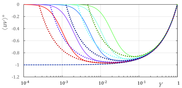
Realizing that the inner-outer overlap of and must coincide and that must be located around its minimum, Sreenivasan, known to his friends as Sreeni, deduced the scaling of the minimum Reynolds stress in several landmark publications, Sreenivasan [10, 11] and Sreenivasan and Sahay [12, fig. 4] as
| (5) |
From equation (4), one immediately deduces the location and value of the minimum Reynolds stress as
| (6) |
Comparing equations (5) and (6) shows that Sreeni’s estimate of , obtained from noisy Reynolds stress minima was amazingly close to present day estimates (see for instance Monkewitz and Nagib [13], henceforth referred to as “MN2023”, and references therein).
The above leading order analysis of the Reynolds stress minimum is supported by the channel DNS of figure 1 “within plotting accuracy”, except for the lowest of 543. However, as will be demonstrated in the following, this is not sufficient to “nail down” to better than , which is believed necessary to definitively settle the question of its flow dependence.
II The near-wall region
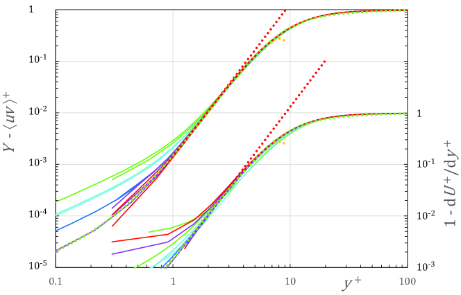
In a first step, the consistency of the Taylor expansions of and of is examined in figure 2 for all the DNS of table 1. The majority of the profiles are seen to be well fitted by the Taylor expansion
Only the profiles #2 and #5 fall significantly below the fit (II) for , but in view of the following cannot be dismissed outright. Note also that below , is dominated by the exact linear term.
As seen in figure 2, the two-term Taylor expansion (II) provides an excellent fit of the data up to around . This range can be extended to beyond 10 by moving, in the spirit of the mean velocity Musker fit[14], to the Padé approximant
Equation (II) may even serve as a rough composite fit, noting however that its asymptotic expansion for is , corresponding to a Kármán parameter of .
III Mean velocity overlap parameters evaluated by fitting asymptotic expansions to and
After concluding in section II, that the Taylor expansions of and of , extracted from the channel DNS of table 1 are, apart from minor question marks, reasonably consistent, the more important question of the Kármán parameter is approached. It can be extracted from either or , which both have the asymptotic expansion
| (9) |
where is the derivative of the linear overlap term of , most recently discussed by MN2023, and is a suitable wake function.
The asymptotic expansion (9) up to the third term, with and , is shown in figure 3 and is seen to fit rather well for . In particular, the linear term in the overlap of , which leads to the offset in equation (9), is clearly visible in the data.
Note here, that a smaller than in MN2023 has been adopted for the expansion (9) in figure 3. This is to better show the problem of fitting equation (9) to the data: As is reduced from its centerline value of , the sum of the first three terms of the asymptotic expansion (9) is seen to first fall below the present DNS data of before crossing the DNS data at . This crossing prevents the asymptotic expansion (9) from being continued beyond the term. To maintain the sum of the first three terms of (9) above and to the left of the DNS data in figure 3 and to “leave room” for the next term , the Kármán parameter would have to be increased beyond , which is higher than most estimates.
A possible fix of the problem is to formulate the log-law derivative in equation (9) with an offset, which is compatible with its asymptotic character, but introduces an additional fitting parameter. In other words, the expansion (9) is modified to
| (10) |
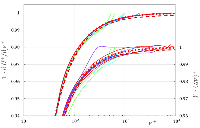
This option is explored in figure 4, which shows that the modified three- and four-term outer expansion (10) provide excellent fits. However, it is not possible to draw any firm conclusions regarding the form of the asymptotic expansion, as long as the glaring discrepancies between and are not clarified. This is the subject of the next section IV, where the discrepancies are magnified by looking at the log-indicator function (1).
IV Overlap parameters evaluated from the log indicator function
After revealing the problems of determining overlap parameters by fitting asymptotic expansions to and in section III, the standard method of looking for constant portions of the log indicator function (1), i.e. for the Kármán “constant”, is investigated next.
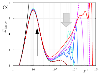
Both variants of the indicator function, and , are shown in figures 5(a) and (b), respectively. It is obvious, that extracting a reliable value for poses problems with both variants. They are however clearly more severe for .
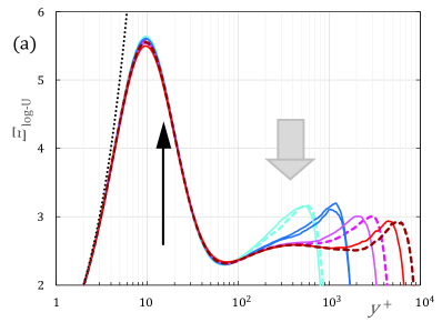
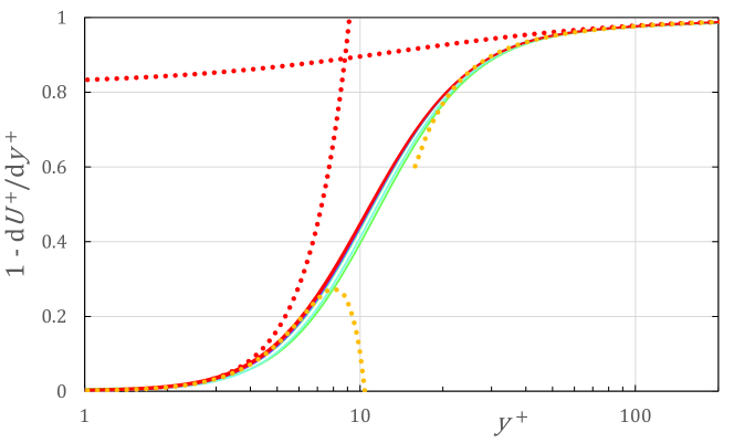
Starting with in figure 5(a), commonly shown in the literature, it has an inner-scaled component independent of in the form of a damped spatial oscillation, to which an outer-scaled linear function is added (see MN2023 and references therein).
As an aside, it is interesting to note, that the locations of the first two maxima of the inner-scaled component correspond approximately to the locations of the inner maximum of at and of its anticipated outer maximum around of 400, both indicated by vertical arrows in the figure. It is furthermore noted, that, if plotted versus (consistent with the scaling of Reynolds stresses[15, 16, 17, 18]), the period of the spatial oscillation becomes approximately constant and the graph starts to look like the spatial version of an under-damped step response in control theory, with the step being the sudden switch-on of the no-slip condition at the wall.
Figure 5(b), on the other hand, shows and reveals large differences relative to as well as between different DNS. Three DNS, #12, 10 and 4, marked by broken lines in figure 5, illustrate three basically different behaviors:
-
-
DNS #12: This is the only DNS considered here, where the outer maximum of at has all but disappeared, which corresponds to an increased anti-correlation of and . The likely cause for this behavior is the unusually small computational box with dimensions of and , which increases the “organisation” of turbulence fluctuations.
-
-
DNS #4: Both indicator functions are identical, apart from some relatively minor oscillations. Only one of the DNS considered here falls into this category and the reasons are not clear.
-
-
DNS #10: The outer maximum of at exceeds 10, i.e. is much higher than the corresponding maximum of . This corresponds to a reduced anti-correlation of and , which is likely related to the rapid increase of wall-normal grid spacing in the outer flow (see e.g. figure 11 of MN2023).
To conclude these observations, it is noted, that the relative consistency of the indicator functions in figure 5(a) (see figure 3 of MN2023 for a more detailed view of its variability) does not necessarily imply that they are representative of perfectly simulated ideal channels. Nevertheless, some confidence may be gained from the excellent collapse of all the DNS in figure 5(a) onto the inner-scaled “damped spatial oscillation” discussed earlier.
Pursuing this line of thought, the approach of MN2023 to extract the inner-scaled part from is implemented, which consists of subtracting the linear fit
| (11) |
from . The result for the DNS considered here is shown in figure 6(a) as solid curves up to and dots beyond, where the are dominated by the wake. The extracted in MN2023 from both channel DNS and experiments is seen to be close to the average between the extrema in figure 6(a) and, although not a plateau of , provides a consistent estimate of even for noisy data.
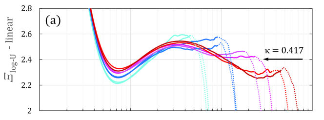
However, the procedure has two weaknesses:
- -
-
-
It also does not completely eliminate the outer-scaled part beyond , i.e. the slope of 1.15 is too low beyond this .
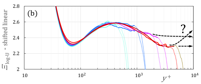
These flaws can be corrected by subtracting a steeper linear function branching off only at :
| (12) |
It is noted in passing that, contrary to in equation (11), becomes exponentially small for and does therefore not contribute to the inner expansion of .
The result, shown in figure 6(b), is seen to produce, for the DNS considered, an excellent collapse of the inner parts of . The figure also shows convincingly, that, over the available range of ’s, this inner part oscillates between 2.3 () and 2.6 () without giving a clear indication on whether it settles to a constant value and, if it does, what the asymptotic might be. Based on the DNS #8 and 10 one might infer an asymptote in figure 6(b) at the level of , while the DNS #11 and 12 suggest higher ’s.
At any rate, figure 6 illustrates why the turbulence community still cannot agree on Kármán “constants”, even without considering indicator functions derived from the Reynolds stress .
V Conclusions
The present extensive data analysis, using both standard and non-standard diagnostics, has uncovered several hitherto unknown or neglected problems with the determination of channel mean velocity overlap parameters, in particular with the slope of the log-law, i.e. the Kármán parameter. Thereby, the focus has been on clear descriptions of the problems and not on proposing still another set of overlap parameters.
In section III the large differences, beyond , between the computed profiles of and of have been documented. The profiles of were found to be sufficiently consistent between the different DNS considered here and have allowed to construct both Taylor and asymptotic expansions. However, it has been shown that, for the usual values of , the origin of the log-law has to be shifted to around -15 in order to be able to continue the asymptotic expansion.
On the other hand, it has not been possible to derive an asymptotic expansion from the different profiles of which are too inconsistent for beyond about 50. This is not entirely surprising, as the evaluation of involves only the separation of the total stream-wise velocity into mean and fluctuating parts, which appears much less sensitive to the specific implementation of a DNS than determining the Reynolds stress.
Section IV, devoted to the analysis of the log indicator function (1), reinforces the conclusions of section III, that the Kármán parameter for channel flow cannot be determined with the desired accuracy from presently available DNS. Worse, all the standard log indicator functions , shown in figure 6, consistently exhibit, after subtracting their outer-scaled linear part, an oscillation with a peak-to-peak amplitude of 0.3 , up to the highest available . This corresponds to oscillating between =.385 and 0.435 !
Several interpretations of and speculations on the oscillations of may be considered:
-
-
The oscillations are an artefact of the implementation of the DNS and in a “perfect” DNS, the inner part of will monotonically approach . This seems rather improbable to the present author, but cannot be completely ruled out.
-
-
In a DNS with significantly reduced residue of the mean momentum equation (3) and , the oscillation in figure 6 becomes more strongly damped and the different indicators converge to a unique specific to the channel. This is this author’s preferred scenario, but requires massive computations at high to confirm.
-
-
It is finally conceivable that, even in DNS of extreme quality, respecting at Reynolds numbers beyond , the oscillations persist. Such an outcome would mean that the log law is only an approximate construct, a sacrilege !
Acknowledgements.
I first met Sreeni in the eighties, standing around a Helium jet in Yale’s Mason lab together with his student Paul Strykowski and discussing absolute instability. Ever since, we have kept in touch and I have always appreciated Sreeni’s openness and the priority of physics in all the technical discussions with him.References
- von Kármán [1930a] T. von Kármán, “Mechanische Ähnlichkeit und Turbulenz,” Nachr. Ges. Wiss. Göttingen, Math. Phys. Klasse 5, 58–76 (1930a).
- von Kármán [1930b] T. von Kármán, “Mechanical similitude and turbulence,” Tech. Rep. TM 611 (NASA, 1930).
- Mil [1938] Proc. 5th Int. Congr. Appl. Mech. (1938) wiley, NY.
- Lee and Moser [2015] M. Lee and R. D. Moser, “Direct numerical simulation of turbulent channel flow up to ,” J. Fluid Mech. 774, 395–415 (2015).
- Abe, Kawamura, and Matsuo [2004] H. Abe, H. Kawamura, and Y. Matsuo, “Surface heat-flux fluctuations in a turbulent channel flow up to =1020 with Pr=0.025 and 0.71,” International Journal of Heat and Fluid Flow 25, 404–419 (2004).
- Hoyas and Jiménez [2006] S. Hoyas and J. Jiménez, “Scaling of the velocity fluctuations in turbulent channels up to ,” Phys. Fluids 18, 011702 (2006).
- Kaneda and Yamamoto [2021] Y. Kaneda and Y. Yamamoto, “Velocity gradient statistics in turbulent shear flow: an extension of Kolmogorov’s local equilibrium theory,” Journal of Fluid Mechanics 929, A13 (2021).
- Lozano-Durán and Jiménez [2014] A. Lozano-Durán and J. Jiménez, “Effect of the computational domain on direct numerical simulations of turbulent channels up to ,” Phys. Fluids 26, 011702 (2014).
- Hoyas et al. [2022] S. Hoyas, M. Oberlack, F. Alcántara-Ávila, S. V. Kraheberger, and J. Laux, “Wall turbulence at high friction Reynolds numbers,” Phys. Rev. Fluids 7, 014602 (2022).
- Sreenivasan [1987] K. R. Sreenivasan, “A unified view of the origin and morphology of the turbulent boundary layer structure,” in Turbulence Management and Relaminarization, edited by H. Liepmann and R. Narasimha (Springer-Verlag, 1987).
- Sreenivasan [1989] K. R. Sreenivasan, “The turbulent boundary layer,” in Frontiers in Experimental Fluid Mechanics, edited by M. Gad-el-Hak (Springer-Verlag, 1989).
- Sreenivasan and Sahay [1997] K. R. Sreenivasan and A. Sahay, “The persistence of viscous effects in the overlap region and the mean velocity in turbulent pipe and channel flows,” in Self-Sustaining Mechanisms of Wall Turbulence, edited by R. L. Panton (Comp. Mech. Publ., Southampton and Boston, 1997) also available as arXiv:physics.flu-dyn/970801.
- Monkewitz and Nagib [2023] P. A. Monkewitz and H. M. Nagib, “The hunt for the Kármán ‘constant’ revisited,” Journal of Fluid Mechanics 967, A15 (2023).
- Musker [1979] A. J. Musker, “Explicit expression for the smooth wall velocity distribution in a turbulent boundary layer,” AIAA J. 17, 655–657 (1979).
- Chen and Sreenivasan [2021] X. Chen and K. R. Sreenivasan, “Reynolds number scaling of the peak turbulence intensity in wall flows,” Journal of Fluid Mechanics 908, R3 (2021).
- Chen and Sreenivasan [2022] X. Chen and K. R. Sreenivasan, “Law of bounded dissipation and its consequences in turbulent wall flows,” Journal of Fluid Mechanics 933, A20 (2022).
- Chen and Sreenivasan [2023] X. Chen and K. R. Sreenivasan, “Reynolds number asymptotics of wall-turbulence fluctuations,” arXiv 2306.02438, to appear in JFM (2023).
- Monkewitz [2023] P. A. Monkewitz, “Reynolds number scaling and inner-outer overlap of stream-wise Reynolds stress in wall turbulence,” arXiv 2307.00612 (2023).