Abstract

Quantum tomography in high-energy physics processes has usually been restricted to the spin degrees of freedom. We address the case of top quark decays $t\to Wb$, in which the angular momentum ($L$) and the spins of $W$ and $b$ are intertwined into a 54-dimensional $LWb$ density operator. The entanglement between $L$ and the $W$ or $b$ spin is large and could be determined for decays of single top quarks produced at the Large Hadron Collider, well above $5\sigma$ (statistical only) from the separability hypothesis. These would be the first entanglement measurements between orbital and spin angular momenta in high-energy physics. The method presented paves the way for similar measurements in other processes.

1 Introduction

Quantum tomography plays a crucial role in our understanding of particle physics processes. By reconstructing the density operator, quantum tomography provides a detailed snapshot of the quantum properties of a system, allowing us to gain insight into its behaviour. The full knowledge of the density operator enables the investigation of quantum entanglement patterns, and can also be used as a novel probe for new physics. For high-energy physics processes, previous literature has focused on the spin degrees of freedom of top quarks [1], $W$ [2] and $Z$ [3] bosons, or combinations of them [4, 5], which can be determined from multi-dimensional angular distributions of their decay products.

Including the orbital angular momentum (hereafter referred to as $L$) is a non-trivial step further because momenta measurement prevents full direct access to its density operator $\rho_{L}$. High-energy physics experiments rely on the measurement of particle momenta, which projects over diagonal states. Specifically, when momenta $P$ are measured the resulting state is $\mathcal{P}\rho_{L}\mathcal{P}$, with $\mathcal{P}=|P\rangle\langle P|$, and different operators $\rho_{L}$ can lead to the same projection $\mathcal{P}\rho_{L}\mathcal{P}$. For the decay of top quarks and other two-body decays, the differential decay width is $d\Gamma\propto\langle\Omega|\rho_{L}|\Omega\rangle$, with $\Omega=(\theta,\phi)$ the flight direction of one of the decay products. $d\Gamma$ involves products of two spherical harmonics evaluated on the same arguments $(\theta,\phi)$, which are not orthogonal functions. Therefore, different operators $\rho_{L}$ may result in the same angular distribution. An extreme case is a scalar, e.g. the Higgs boson, where the decay distribution is isotropic despite $\rho_{L}$ contains non-zero entries $|l\,m\rangle\langle l^{\prime}\,m^{\prime}|$, up to $l,l^{\prime}=2$ in the decay to vector bosons and $l,l^{\prime}=1$ in the decay to fermions.

In this Letter we consider a case of interest, the decay of top quarks $t\to Wb$, to address the determination of the 54-dimensional $LWb$ density operator that completely describes angular momentum in the top quark decay. We make a novel use of the complementarity between ‘canonical’ decay amplitudes, calculated using a fixed quantisation axis for all particles, and helicity amplitudes, in which the spin of the decay products is quantised in their direction of motion. While the former are the key tool to write down the $LWb$ density operator, the latter are very convenient to extract from multi-dimensional angular decay distributions the independent parameters that govern the top decay. The $LW$ and $Lb$ density operators are also of interest: they exhibit a large entanglement between the orbital and spin angular momentum parts, which can be experimentally determined, with a caveat that will be discussed. Previous experimental measurements of entanglement between orbital and spin angular momenta have been limited to photon pairs, see for example Refs. [6, 7].

2 Framework

In the top quark rest frame we take a fixed reference system $(x,y,z)$ and parameterise the three-momentum of the $W$ boson as

$$\vec{p}=q(\sin\theta\cos\phi,\sin\theta\sin\phi,\cos\theta)\,.$$ (1)

Within the helicity amplitude framework of Jacob and Wick [8], angular momentum conservation implies that for the $t\to Wb$ decay the helicity amplitudes must have the form

$$A^{h}_{M\lambda_{1}\lambda_{2}}(\theta,\phi)=a_{\lambda_{1}\lambda_{2}}D_{M\lambda}^{1/2\,*}(\phi,\theta,0)\,,$$ (2)

with $M$ the third spin component of $t$, $\lambda_{1}$ and $\lambda_{2}$ the helicities of $W$ and $b$, respectively, and $\lambda=\lambda_{1}-\lambda_{2}$. $D^{J}_{m^{\prime}m}$ are the Wigner functions and the ‘reduced amplitudes’ $a_{\lambda_{1}\lambda_{2}}$ are constants that do not depend on the angles, the only non-zero ones being $a_{1\frac{1}{2}}$, $a_{0\frac{1}{2}}$, $a_{0-\frac{1}{2}}$, $a_{-1-\frac{1}{2}}$. The combinations $\lambda_{1}=1$, $\lambda_{2}=-1/2$ and $\lambda_{1}=-1$, $\lambda_{2}=1/2$ are not allowed by angular momentum conservation, because the $L$ component in the direction of motion $\vec{p}$ vanishes. Performing a change of basis for the $b$ spinors and the $W$ polarisation vectors one can obtain the canonical amplitudes $A^{c}_{Ms_{1}s_{2}}(\theta,\phi)$, in which the $W$ and $b$ spins are quantised in the $\hat{z}$ axis, with respective eigenvalues $s_{1}$ and $s_{2}$. Expanding them in terms of spherical harmonics $Y_{l}^{m}$, and bearing in mind that $\langle\Omega|lm\rangle=Y_{l}^{m}(\Omega)$, the amplitudes $A_{Ms_{1}s_{2};lm}$ into $|lm\rangle$ eigenstates can be identified. The non-zero ones are

$$A_{\frac{1}{2}1\frac{1}{2};1-1}=A_{-\frac{1}{2}-1-\frac{1}{2};11}=\sqrt{\frac{\pi}{6}}\mathcal{F}_{1}^{-}\,,$$

$$A_{\frac{1}{2}1\frac{1}{2};2-1}=-A_{-\frac{1}{2}-1-\frac{1}{2};21}=\sqrt{\frac{\pi}{30}}\mathcal{F}_{2}\,,$$

$$A_{\frac{1}{2}0\frac{1}{2};00}=-A_{-\frac{1}{2}0-\frac{1}{2};00}=\sqrt{\frac{\pi}{9}}\mathcal{F}_{0}\,,$$

$$A_{\frac{1}{2}0\frac{1}{2};10}=A_{-\frac{1}{2}0-\frac{1}{2};10}=\sqrt{\frac{\pi}{3}}\mathcal{F}_{1}^{0}\,,$$

$$A_{\frac{1}{2}0\frac{1}{2};20}=-A_{-\frac{1}{2}0-\frac{1}{2};20}=-\sqrt{\frac{2\pi}{45}}\mathcal{F}_{2}\,,$$

$$A_{\frac{1}{2}-1\frac{1}{2};11}=A_{-\frac{1}{2}1-\frac{1}{2};1-1}=\sqrt{\frac{\pi}{6}}\mathcal{F}_{1}^{+}\,,$$

$$A_{\frac{1}{2}-1\frac{1}{2};21}=-A_{-\frac{1}{2}1-\frac{1}{2};2-1}=\sqrt{\frac{\pi}{30}}\mathcal{F}_{2}\,,$$

$$A_{\frac{1}{2}1-\frac{1}{2};00}=-A_{-\frac{1}{2}-1\frac{1}{2};00}=-\sqrt{\frac{2\pi}{9}}\mathcal{F}_{0}\,,$$

$$A_{\frac{1}{2}1-\frac{1}{2};10}=A_{-\frac{1}{2}-1\frac{1}{2};10}=\sqrt{\frac{\pi}{3}}\mathcal{F}\,,$$

$$A_{\frac{1}{2}1-\frac{1}{2};20}=-A_{-\frac{1}{2}-1\frac{1}{2};20}=-\sqrt{\frac{\pi}{45}}\mathcal{F}_{2}\,,$$

$$A_{\frac{1}{2}0-\frac{1}{2};11}=A_{-\frac{1}{2}0\frac{1}{2};1-1}=-\sqrt{\frac{\pi}{3}}\mathcal{F}\,,$$

$$A_{\frac{1}{2}0-\frac{1}{2};21}=-A_{-\frac{1}{2}0\frac{1}{2};2-1}=\sqrt{\frac{\pi}{15}}\mathcal{F}_{2}\,,$$

$$A_{\frac{1}{2}-1-\frac{1}{2};22}=-A_{-\frac{1}{2}1\frac{1}{2};2-2}=-\sqrt{\frac{2\pi}{15}}\mathcal{F}_{2}\,.$$ (3)

We have introduced the combinations

$$\mathcal{F}=a_{-1-\frac{1}{2}}-a_{1\frac{1}{2}}\,,\quad\mathcal{F}_{1}^{0}=a_{0-\frac{1}{2}}-a_{0\frac{1}{2}}\,,$$

$$\mathcal{F}_{0}=\sqrt{2}(a_{1\frac{1}{2}}+a_{-1-\frac{1}{2}})+a_{0\frac{1}{2}}+a_{0-\frac{1}{2}}\,,$$

$$\mathcal{F}_{1}^{\pm}=\pm(a_{-1-\frac{1}{2}}-a_{1\frac{1}{2}})+\sqrt{2}(a_{0\frac{1}{2}}-a_{0-\frac{1}{2}})\,,$$

$$\mathcal{F}_{2}=a_{-1-\frac{1}{2}}+a_{1\frac{1}{2}}-\sqrt{2}(a_{0\frac{1}{2}}+a_{0-\frac{1}{2}})\,.$$ (4)

The amplitudes in (3) are completely general, and the relation with $a_{\lambda_{1}\lambda_{2}}$ holds for any two-body decay of a spin-$1/2$ particle into massive spin-1 and spin-$1/2$ particles. For the top quark decay one can use the helicity amplitudes calculated in [9] for a generic interaction

$$\mathcal{L}=-\frac{1}{\sqrt{2}}\bar{b}\gamma^{\mu}(g_{L}P_{L}+g_{R}P_{R})t\,W_{\mu}^{-}$$ (5)

and match them to the general form (2), to obtain for this specific case the reduced amplitudes (or just amplitudes, for brevity)

$$a_{1\frac{1}{2}}=\frac{1}{\sqrt{2}}(g_{L}H_{1}^{-}-g_{R}H_{1}^{+})\,,$$

$$a_{0\frac{1}{2}}=\frac{1}{\sqrt{2}}(g_{L}H_{1}^{-}H_{2}^{-}-g_{R}H_{1}^{+}H_{2}^{+})\,,$$

$$a_{0-\frac{1}{2}}=\frac{1}{\sqrt{2}}(g_{L}H_{1}^{+}H_{2}^{+}-g_{R}H_{1}^{-}H_{2}^{-})\,,$$

$$a_{-1-\frac{1}{2}}=\frac{1}{\sqrt{2}}(g_{L}H_{1}^{+}-g_{R}H_{1}^{-})\,,$$ (6)

with

$$H_{1}^{\pm}=[m_{t}(E_{b}+m_{b})]^{1/2}\left(1\pm\frac{q}{E_{b}+m_{b}}\right)\,,$$

$$H_{2}^{\pm}=\frac{E_{W}\pm q}{\sqrt{2}M_{W}}\,.$$ (7)

The masses of $t$, $W$ and $b$ are denoted as $m_{t}$, $M_{W}$ and $m_{b}$, as usual, and $E_{W}$, $E_{b}$ are the energies of $W$ and $b$, respectively, in the top quark rest frame. As a cross check, plugging (6) into (3) and using $\langle\Omega|lm\rangle=Y_{l}^{m}(\Omega)$, one recovers the canonical amplitudes $A^{c}_{Ms_{1}s_{2}}(\theta,\phi)$ obtained in [10] by direct calculation. Within the Standard Model (SM), and using $m_{t}=172.5$ GeV, $M_{W}=80.4$ GeV, $m_{b}=4.8$ GeV, one finds $(a_{1\frac{1}{2}},a_{0\frac{1}{2}},a_{0-\frac{1}{2}},a_{-1-\frac{1}{2}})=g(5.4,1.8,231,153)$ GeV, with $g$ the electroweak constant. The amplitudes with $\lambda_{2}=1/2$ are suppressed because the $tbW$ interaction is left-handed and the $b$ quark is much lighter than the top quark.

3 Density operators for top quark decay

Given a density operator

$$\rho_{t}=\frac{1}{2}\left(\!\begin{array}[]{cc}1+P_{3}&P_{1}-iP_{2}\\ P_{1}+iP_{2}&1-P_{3}\end{array}\!\right)$$ (8)

describing the spin state of the decaying top quarks, the $LWb$ density operator $\rho_{LWb}$ for its decay products is

$$(\rho_{LWb})_{s_{1}s_{2};lm}^{s_{1}^{\prime}s_{2}^{\prime};l^{\prime}m^{\prime}}=(\rho_{t})_{MM^{\prime}}A_{Ms_{1}s_{2};lm}A_{M^{\prime}s_{1}^{\prime}s_{2}^{\prime};l^{\prime}m^{\prime}}^{*}\,,$$ (9)

with a sum over $M,M^{\prime}$. Taking the partial trace over the $b$ spin, $W$ spin or $L$ subspaces we obtain the density operators $\rho_{LW}$, $\rho_{Lb}$ and $\rho_{Wb}$, respectively. For these bipartite systems the entanglement can be characterised by the Peres-Horodecki [11, 12] criterion: for a density operator $\rho$ that describes a bipartite system $AB$, the positivity of the partial transpose over any subsystem, say $\rho^{T_{B}}$, is a necessary condition for separability. Conversely, a non-positive $\rho^{T_{B}}$ is a sufficient condition for entanglement. The amount of entanglement can be quantified by the negativity of the partial transpose on the $B$ subspace $\rho^{T_{B}}$ [13],

$$N(\rho)=\frac{\|\rho^{T_{B}}\|-1}{2}\,,$$ (10)

where $\|X\|=\operatorname{tr}\sqrt{XX^{\dagger}}=\sum_{i}\sqrt{\lambda_{i}}$, where $\lambda_{i}$ are the (positive) eigenvalues of the matrix $XX^{\dagger}$. Because $\rho^{T_{B}}$ has unit trace, $N(\rho)$ equals the sum of the negative eigenvalues of $\rho^{T_{B}}$. (The result is the same when taking the partial transpose on subsystem $A$.) In the separable case $N(\rho)=0$. As an example, in the SM we have for the decay of top quarks in a $S_{3}=1/2$ eigenstate $N(\rho_{LW})=0.615$, $N(\rho_{Lb})=0.396$, $N(\rho_{Wb})=0.010$, i.e. all the pairs of subsystems are entangled when tracing on the remaining one. Note, however, that $\rho_{Wb}$ is separable in the $m_{b}=0$ limit, because in that case the $b$ quarks have left-handed helicity and there are only two non-zero $a_{\lambda_{1}\lambda_{2}}$, those with $\lambda_{2}=-1/2$. For unpolarised top quarks we have $N(\rho_{LW})=0.432$, $N(\rho_{Lb})=0.353$, $N(\rho_{Wb})=0$.

4 Parameter determination

Single top quarks are produced at the Large Hadron Collider (LHC) in the process $pp\to t\bar{b}j$ with a large polarisation in the direction of the spectator jet $j$. As shown in Ref. [14], this allows to determine $a_{\lambda_{1}\lambda_{2}}$, except for (i) a global normalisation that does not affect the density operators, and is set to unity; (ii) the relative phase $e^{i\alpha}$ between $\lambda_{2}=1/2$ and $\lambda_{2}=-1/2$ amplitudes, which has a marginal effect on the $LW$ and $Lb$ entanglement. In addition to the $(\theta,\phi)$ angles previously introduced for the top quark decay, to measure $W$ spin observables one has to consider the angles $(\theta^{*},\phi^{*})$ describing the orientation of the charged lepton momentum in the $W$ rest frame, with respect to a $(x^{\prime},y^{\prime},z^{\prime})$ system where the $\hat{z}^{\prime}$ axis is in the direction of $\vec{p}$ and the $\hat{y}^{\prime}$ angle lies in the $xy$ plane making an angle $\phi$ with the $\hat{y}$ axis.

The top quark polarisation, namely $P_{1-3}$, is determined by using the charged lepton as spin analyser [1]. We use forward-backward (FB) asymmetries on $\cos\theta_{\hat{n}}$, with $\theta_{\hat{n}}$ the angle between the charged lepton momentum in the top quark rest frame and an arbitrary axis $\hat{n}$. Their relation to the top quark polarisation $P_{\hat{n}}$ in that axis is

$$A_{\text{FB}}^{\hat{n}}=\frac{P_{\hat{n}}}{2}\,.$$ (11)

For the determination of $a_{\lambda_{1}\lambda_{2}}$ we use a simple set of observables. The well-known $W$ helicity fractions [1] $F_{\pm}$, $F_{0}$ can be determined from a fit to the $\cos\theta^{*}$ distribution,

$$\frac{1}{\Gamma}\frac{d\Gamma}{d\cos\theta^{*}}=\frac{3}{8}F_{+}(1+\cos\theta^{*})^{2}+\frac{3}{4}F_{0}\sin^{2}\theta^{*}+\frac{3}{8}F_{-}(1-\cos\theta^{*})^{2}\,.$$ (12)

Their relation to $a_{\lambda_{1}\lambda_{2}}$ is

$$F_{+}=|a_{1\frac{1}{2}}|^{2}\,,\quad F_{-}=|a_{-1-\frac{1}{2}}|^{2}\,,\quad F_{0}=|a_{0\frac{1}{2}}|^{2}+|a_{0-\frac{1}{2}}|^{2}\,.$$ (13)

The two amplitudes with $\lambda_{1}=0$ can be disentangled with a forward-backward central-edge asymmetry [14] on the quantity $\cos\theta(|\cos\theta^{*}|-t)$, with $t=(1+\sqrt{2})^{1/3}-(1+\sqrt{2})^{-1/3}$,

$$A_{\text{FB,EC}}^{z,z^{\prime}}=\frac{3}{2}(2t-1)P_{3}\left[|a_{0\frac{1}{2}}|^{2}-|a_{0-\frac{1}{2}}|^{2}\right]\,.$$ (14)

The two phases between like-$\lambda_{2}$ amplitudes can be measured from FB asymmetries $A^{x^{\prime}}$, $A^{y^{\prime}}$, $A^{x^{\prime}z^{\prime}}$, $A^{y^{\prime}z^{\prime}}$ built on the quantities $\cos\phi^{*}$, $\sin\phi^{*}$, $\cos\phi^{*}\cos\theta^{*}$ and $\sin\phi^{*}\cos\theta^{*}$, respectively  [14]

$$A_{\text{FB}}^{x^{\prime}}=-\frac{3\pi}{8\sqrt{2}}P_{3}\operatorname{Re}\left[a_{0\frac{1}{2}}a_{1\frac{1}{2}}^{*}+a_{-1-\frac{1}{2}}a_{0-\frac{1}{2}}^{*}\right]\,,$$

$$A_{\text{FB}}^{y^{\prime}}=-\frac{3\pi}{8\sqrt{2}}P_{3}\operatorname{Re}\left[a_{0\frac{1}{2}}a_{1\frac{1}{2}}^{*}+a_{-1-\frac{1}{2}}a_{0-\frac{1}{2}}^{*}\right]\,,$$

$$A_{\text{FB}}^{x^{\prime}z^{\prime}}=-\frac{1}{2\sqrt{2}}P_{3}\operatorname{Re}\left[a_{0\frac{1}{2}}a_{1\frac{1}{2}}^{*}-a_{-1-\frac{1}{2}}a_{0-\frac{1}{2}}^{*}\right]\,,$$

$$A_{\text{FB}}^{y^{\prime}z^{\prime}}=-\frac{1}{2\sqrt{2}}P_{3}\operatorname{Re}\left[a_{0\frac{1}{2}}a_{1\frac{1}{2}}^{*}-a_{-1-\frac{1}{2}}a_{0-\frac{1}{2}}^{*}\right]\,.$$ (15)

Finally, the relative phase between $\lambda_{2}=1/2$ and $\lambda_{2}=-1/2$ amplitudes cannot be measured as long as the $b$ quark polarisation is not currently accessible in the ATLAS and CMS experiments. However, its impact is marginal because $\lambda_{2}=1/2$ amplitudes are quite suppressed. For top quarks in a $S_{3}=1/2$ eigenstate, and using the SM values for $a_{\lambda_{1}\lambda_{2}}$ but inserting an arbitrary relative phase $e^{i\alpha}$ in $a_{1\frac{1}{2}}$ and $a_{0\frac{1}{2}}$, $N(\rho_{LW})$ lies in the range $[0.614,0.628]$ and $N(\rho_{Lb})$ in the range $[0.396,0.411]$. The minimum entanglement is found for the SM value of the phase, $\alpha=0$. This variation, of the order of the expected statistical uncertainty, is not relevant for the determination of the $LW$ and $Lb$ entanglement.

5 Experimental sensitivity

We estimate the statistical sensitivity for the determination of the entanglement measures $N(\rho_{LW})$ and $N(\rho_{Lb})$ with the data collected at the LHC Run 2, working at the partonic level. An event sample is generated with MadGraph [15], in the process $pp\to t\bar{b}j$, using NNPDF 3.1 [16] parton density functions and setting as factorisation and renormalisation scale the average transverse mass. (Top anti-quarks are not included.) The resulting top quark polarisation is $P_{3}=0.845$ in the spectator jet axis, with $P_{1}=0.035$, $P_{2}=0$ in orthogonal directions [17, 18]. We perform pseudo-experiments, in which (i) a subset of events is randomly chosen; (ii) the values of $P_{i}$ and $a_{\lambda_{1}\lambda_{2}}$ are determined from the set; (iii) the density operators are reconstructed using Eqs. (3) and (9); (iv) the entanglement measures are computed for the $LW$ and $Lb$ operators. For each pseudo-experiment we take a sample of 50000 events, which is the expected number of the events after selection cuts in the single top polarisation measurement performed by the ATLAS Collaboration [18] with the full Run 2 luminosity (139 fb^-1). The relative phase that cannot be measured is set to its SM value, $\alpha=0$. Using a non-SM value increases $N(\rho_{LW})$ up to $0.013$ and $N(\rho_{Lb})$ up to $0.017$.

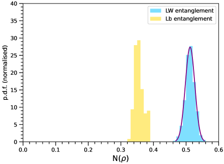
Figure 1: Distribution of $LW$ and $Lb$ entanglement measures $N$ obtained from pseudo-experiments. The curve shows a Gaussian fit to the $N(\rho_{LW})$ distribution in the interval $[-3\sigma,3\sigma]$.

The result of 20000 pseudo-experiments is presented in Fig. 1. For $LW$ entanglement the distribution is Gaussian to a good approximation, and the expected statistical precision is $N(\rho_{LW})=0.512\pm 0.015$. For $Lb$ entanglement the distribution presents a small shoulder caused by the boundary condition $F_{+}\geq 0$. In this case, the mean is $\langle N(\rho_{Lb})\rangle=0.356$ and the standard deviation is $0.014$. In both cases, the measurements have a statistical precision that would allow to establish the entanglement ($N>0$) beyond the $5\sigma$ criterion, nominally 35 and 25 standard deviations.

6 Discussion

The reader may already have noticed two conspicuous features that arise in our theoretical framework. The $LW$ density operator, obtained after trace on the $b$ spin degrees of freedom, is still sensitive to the phase $e^{i\alpha}$ between amplitudes with $b$ quark helicities $\pm 1/2$. This is a consequence of the ambiguity in the direct determination of the density operators involving $L$, which we solve by expressing them in terms of $a_{\lambda_{1}\lambda_{2}}$. Even more striking is the fact that the $Lb$ entanglement can be established when the $b$ quark spin cannot be directly measured. This is possible due the change of basis used to write the $LWb$ density operator in terms of a minimal set of parameters $a_{\lambda_{1}\lambda_{2}}$, and the fact that $\lambda=1/2$ are suppressed.

The excellent statistical sensitivity expected for these entanglement measurements suggests that they will be limited by systematic uncertainties. For the single top polarisation, the Run 2 ATLAS measurement [18], which used a multi-dimensional template fit, has uncertainties of 17%, 2.5% and 10%, for $P_{1}$, $P_{2}$ and $P_{3}$, respectively. The measurements of the $W$ helicity fractions by the CMS Collaboration in single top production with Run 1 data [19] have systematic uncertainties below 4%. Asymmetries equivalent to $A_{\text{FB}}^{x^{\prime}}$, $A_{\text{FB}}^{y^{\prime}}$, $A_{\text{FB}}^{x^{\prime}z^{\prime}}$, $A_{\text{FB}}^{y^{\prime}z^{\prime}}$ have been measured by the ATLAS Collaboration in single top production with Run 1 data [20] with systematics of 8%, 3%, 11% and 5%, respectively. A measurement of $A_{\text{FB,EC}}^{z,z^{\prime}}$ has not been performed yet. It requires reconstruction of the $\hat{z}$ axis (spectator jet) and $\hat{z}^{\prime}$ axis ($W$ momentum). In both cases the directions are well determined, so we expect a systematic uncertainty at the 10% level, as obtained for $P_{3}$. We also remark that with high statistics, as those available with Run 2 data, the full distributions can be used for measurements, not only asymmetries. With that purpose, a deconvolution of the detector effects for measurements of the four-dimensional distribution has been proposed [21, 22], which also takes into account the correlations among measurements.

In summary, the determination of the $LW$ and $Lb$ entanglement is based on observables which, except one, have already been measured by the ATLAS or CMS Collaborations, in separate analyses. The current experimental uncertainties suggest that a dedicated analysis of Run 2 data could establish the entanglement between $L$ and the $W$ boson spin, or $L$ and the $b$ quark spin, with more than 5 standard deviations.

References

- [1] G. L. Kane, G. A. Ladinsky and C. P. Yuan, “Using the Top Quark for Testing Standard Model Polarization and CP Predictions,” Phys. Rev. D 45, 124-141 (1992)
- [2] J. A. Aguilar-Saavedra and J. Bernabéu, “Breaking down the entire boson spin observables from its decay,” Phys. Rev. D 93, no.1, 011301 (2016) [arXiv:1508.04592 [hep-ph]].
- [3] J. A. Aguilar-Saavedra, J. Bernabéu, V. A. Mitsou and A. Segarra, “The boson spin observables as messengers of new physics,” Eur. Phys. J. C 77, no.4, 234 (2017) [arXiv:1701.03115 [hep-ph]].
- [4] R. Rahaman and R. K. Singh, “Breaking down the entire spectrum of spin correlations of a pair of particles involving fermions and gauge bosons,” Nucl. Phys. B 984, 115984 (2022) [arXiv:2109.09345 [hep-ph]].
- [5] A. Bernal, “Quantum tomography of helicity states for general scattering processes,” [arXiv:2310.10838 [hep-ph]].
- [6] T. Stav et al., ‘Quantum entanglement of the spin and orbital angular momentum of photons using metamaterials”, Science 361 (2018) 1101.
- [7] R. Fickler, G. Campbell, B. Buchler, P. K. Lam and A. Zeilinger, “Quantum entanglement of angular momentum states with quantum numbers up to 10,010,” Proc. Nat. Acad. Sci. 113, no.48, 13642 (2016)
- [8] M. Jacob and G. C. Wick, “On the General Theory of Collisions for Particles with Spin,” Annals Phys. 7, 404-428 (1959)
- [9] J. A. Aguilar-Saavedra and J. A. Casas, “Entanglement autodistillation from particle decays,” [arXiv:2401.06854 [hep-ph]].
- [10] J. A. Aguilar-Saavedra, “A closer look at post-decay entanglement,” [arXiv:2401.10988 [hep-ph]].
- [11] A. Peres, “Separability criterion for density matrices,” Phys. Rev. Lett. 77, 1413-1415 (1996) [arXiv:quant-ph/9604005 [quant-ph]].
- [12] P. Horodecki, “Separability criterion and inseparable mixed states with positive partial transposition,” Phys. Lett. A 232, 333 (1997) [arXiv:quant-ph/9703004 [quant-ph]].
- [13] M. B. Plenio and S. Virmani, “An introduction to entanglement measures,” Quant. Inf. Comput. 7, no.1-2, 001-051 (2007) [arXiv:quant-ph/0504163 [quant-ph]].
- [14] J. A. Aguilar-Saavedra, J. Boudreau, C. Escobar and J. Mueller, “The fully differential top decay distribution,” Eur. Phys. J. C 77, no.3, 200 (2017) [arXiv:1702.03297 [hep-ph]].
- [15] J. Alwall, R. Frederix, S. Frixione, V. Hirschi, F. Maltoni, O. Mattelaer, H. S. Shao, T. Stelzer, P. Torrielli and M. Zaro, “The automated computation of tree-level and next-to-leading order differential cross sections, and their matching to parton shower simulations,” JHEP 07, 079 (2014) [arXiv:1405.0301 [hep-ph]].
- [16] R. D. Ball et al. [NNPDF], “Parton distributions from high-precision collider data,” Eur. Phys. J. C 77, no.10, 663 (2017) [arXiv:1706.00428 [hep-ph]].
- [17] J. A. Aguilar-Saavedra and S. Amor Dos Santos, “New directions for top quark polarization in the -channel process,” Phys. Rev. D 89, no.11, 114009 (2014) [arXiv:1404.1585 [hep-ph]].
- [18] G. Aad et al. [ATLAS], “Measurement of the polarisation of single top quarks and antiquarks produced in the t-channel at = 13 TeV and bounds on the dipole operator from the ATLAS experiment,” JHEP 11, 040 (2022) [arXiv:2202.11382 [hep-ex]].
- [19] V. Khachatryan et al. [CMS], “Measurement of the W boson helicity in events with a single reconstructed top quark in pp collisions at TeV,” JHEP 01, 053 (2015) [arXiv:1410.1154 [hep-ex]].
- [20] M. Aaboud et al. [ATLAS], “Probing the vertex structure in t-channel single-top-quark production and decay in pp collisions at TeV with the ATLAS detector,” JHEP 04, 124 (2017) [arXiv:1702.08309 [hep-ex]].
- [21] J. Boudreau, C. Escobar, J. Mueller, K. Sapp and J. Su, “Single top quark differential decay rate formulae including detector effects,” [arXiv:1304.5639 [hep-ex]].
- [22] J. Boudreau, C. Escobar, J. Mueller and J. Su, “Deconvolving the detector in Fourier space,” J. Phys. Conf. Ser. 762, no.1, 012041 (2016)