Rotating Rayleigh-Bénard convection: Attractors, bifurcations and heat transport via a Galerkin hierarchy

Abstract.

Motivated by the need for energetically consistent climate models, the Boussinessq-Coriolis (BC) equations are studied with a focus on the Nusselt number, defined as the averaged vertical heat transport. The Howard-Krishnamurthy-Coriolis (HKC) hierarchy is defined by explicitly computing the Galerkin truncations and selecting the Fourier modes in a particular way, such that this hierarchy can be shown to energy relations consistent with the PDE. Well-posedness and the existence of an attractor are then proven for the BC model, and an explicit upper bound on the attractor dimension is given. By studying the local bifurcations at the origin, a lower bound on the attractor dimension is provided. Finally, a series of numerical studies are performed by implementing the HKC hierarchy in MATLAB, which investigate convergence of the Nusselt number as one ascends HKC hierarchy as well as other issues related to heat transport parameterization.

1. Introduction

In the study of climate, general circulation models aim to accurately represent the motions of the atmosphere and ocean using equations from fluid dynamics. However, vertical accelerations are often set equal to zero in primitive equation models. This assumption is partially justified from a physical viewpoint, since the vertical accelerations should be small compared to more dominant forces (gravity, etc) which are in an approximate hydrostatic balance. Furthermore, this yields a significant mathematical benefit since the well-posedness theory for such equations is then much more satisfactory [1]. On the other hand, such an assumption cannot be entirely physically accurate, and hence often in the climate community additional terms are included to account for the discrepancy. This procedure is known as parameterization, and there is not a consensus about a correct or optimal way to parameterize convection [8]. Hence the main goal of this paper is to develop a mathematically rigorous framework for studying vertical heat transport in turbulent convection. An eventual goal is to assess the quality of different parameterizations for atmospheric convection, although a full assessment is beyond the scope of this paper.

The models considered in this paper are the three-dimensional, non-dimensionalized Boussinesq Oberbeck equations with a Coriolis force

(1) $$\begin{split}\frac{1}{\mathsf{P}}\Big{[}\partial_{t}\textbf{u}+\textbf{u}\cdot\nabla\textbf{u}\Big{]}+\nabla p&=\Delta\textbf{u}+\pi\mathcal{R}T\hat{e}_{3}-\mathscr{R}\hat{e}_{3}\times\textbf{u}\\ \nabla\cdot\textbf{u}&=0\\ \partial_{t}T+\textbf{u}\cdot\nabla T&=\Delta T,\end{split}$$

and its Galerkin truncations. Here $\textbf{u}=(u_{1},u_{2},u_{3})$, $T$, $p$ are the non-dimensionalized velocity, temperature and pressure of a fluid lying in a box $\textbf{x}=(x_{1},x_{2},x_{3})\in[0,\frac{2\pi}{k_{1}}]\times[0,\frac{2\pi}{k_{2}}]\times[0,\pi]$ for box parameters $k_{i}$. The fluid is assumed to be periodic in $x_{1},x_{2}$ and in order to simplify the analysis, it is assumed that the fluid configuration is horizontally aligned, ie it is independent of the variable $x_{2}$. This assumption is invariant under the full three dimension evolution, although small perturbations from perfect alignment will typically destroy this condition. Due to this condition it suffices to consider the behavior on the plane $x_{2}=0$, hence the domain is taken to be $\Omega=[0,\frac{2\pi}{k_{1}}]\times[0,\pi]$. The fluid is assumed to be heated from below and cooled from above, hence the non-dimensionalized temperature $T$ must satisfy the boundary conditions

(2) $$T(x_{1},0,t)=1\hskip 28.45274pt\text{ , }\hskip 28.45274ptT(x_{1},\pi,t)=0.$$

Furthermore, the fluid is assumed to satisfy the impenetrability and free slip conditions at the top and bottom boundaries

(3) $$u_{3}=0\hskip 28.45274pt\text{ , }\hskip 28.45274pt\partial_{x_{3}}u_{1}=\partial_{x_{3}}u_{2}=0\hskip 56.9055pt\text{ for }\hskip 14.22636ptx_{3}=0,1.$$

The parameters $\mathsf{P},\mathcal{R}$ are the Prandtl and Rayleigh numbers, whereas the rotation number $\mathscr{R}$ is proportional to the angular velocity of the moving frame. If the fluid is supposed to represent air in order to model atmospheric convection, and furthermore the domain is taken to be the troposphere then by plugging in approximate values as in Appendix A one finds that the relevant parameter values are approximately as follows:

(4) $$\mathsf{P}\approx\mathscr{O}(1)\hskip 28.45274pt\text{ , }\hskip 28.45274pt\mathcal{R}\approx\mathscr{O}(10^{15})\hskip 28.45274pt\text{ , }\hskip 28.45274pt\mathscr{R}\approx 0-\mathscr{O}(10^{6}).$$

As described, the main quantity of interest is average vertical heat transport, as measured by the Nusselt number. Using the notation $\langle\cdot\rangle$ to denote the volume integral, and an overbar to denote an infinite time average

$$\langle f\rangle:=\int_{\Omega}f(\textbf{x})d\textbf{x}\hskip 14.22636pt\text{ , }\hskip 14.22636pt\bar{f}:=\lim_{t\to\infty}\frac{1}{t}\int_{0}^{t}f(s)ds,$$

the Nusselt number is then defined as the vertical heat flux in the domain, averaged over time and space:

(5) $$\mathsf{Nu}:=1+\frac{k_{1}}{2\pi^{2}}\overline{\langle u_{3}T\rangle}.$$

Apriori, the Nusselt number depends in a complicated way on the initial states $(\textbf{u}_{0},T_{0})$, and the parameters, $\mathcal{R},\mathsf{P},\mathscr{R},k_{1}$. Often of primary interest is the dependence of the Nusselt number on the Rayleigh number, and often the other parameters are held constant. While there have been numerous numerical studies about this dependence [29, 30, 17, 25], there are relatively few analytical results. These analytic results regard universal upper bounds on the Nusselt number applying to all $(\textbf{u}_{0},T_{0})$ and varying with $\mathcal{R}\geq 0$. The standard approach here is the background field method, originally developed by Constantin and Doering [7], which consists of three main steps. First, one uses the PDE to establish balance laws such as those for the kinetic and potential energy, which then imply equalities between infinite time averages:

(6) $$\begin{split}\frac{d}{dt}\langle\frac{1}{2}|\textbf{u}|^{2}\rangle&=-\mathsf{P}\langle|\nabla\textbf{u}|^{2}\rangle+\pi\mathsf{P}\mathcal{R}\langle u_{3}T\rangle\hskip 42.67912pt\Rightarrow\hskip 42.67912pt-\mathsf{P}\overline{\langle|\nabla\textbf{u}|^{2}\rangle}+\pi\mathsf{P}\mathcal{R}\overline{\langle u_{3}T\rangle}=0,\\ \frac{d}{dt}\langle(1-\frac{x_{3}}{\pi})T\rangle&=-\frac{1}{\pi}\langle u_{3}T\rangle+\langle(1-\frac{x_{3}}{\pi})\partial_{x_{3}}^{2}T\rangle\hskip 28.45274pt\Rightarrow\hskip 42.67912pt-\frac{1}{\pi}\overline{\langle u_{3}T\rangle}+\overline{\langle(1-\frac{x_{3}}{\pi})\partial_{x_{3}}^{2}T\rangle}=0.\end{split}$$

One then rewrites the temperature as $T=\zeta(x_{3})+\theta(x_{1},x_{2},t)$, where $\zeta$ is some undetermined background field and $\theta$ is a fluctuation, uses the infinite time average equalities to rewrite the Nusselt number and uses calculus of variations arguments to choose the background field which optimizes the resulting bound. This method provides sharpest known bound in the non-rotating, free slip case [31], namely that for fixed $\mathsf{P},k_{1}$ there exists a constant $C_{\mathsf{P},k_{1}}$ such that

$$\hskip 113.81102pt\sup_{(\textbf{u}_{0},T_{0})}\mathsf{Nu}\leq 1+C_{\mathsf{P},k_{1}}\mathcal{R}^{5/12}\hskip 56.9055pt\text{ for all}\hskip 7.11317pt\mathcal{R}\geq 0.$$

Less is known when both the dependence on the rotation and Rayleigh numbers are considered. To the best of the author’s knowledge the only analytical result here was obtained by Constantin et al. [4, 5] in the special case where $\mathsf{P}=\infty$, hence far from the parameter regime for atmospheric flows, who showed that there exists a constant $C$ such that

$$\sup_{(\textbf{u}_{0},T_{0})}\mathsf{Nu}\leq\left\{\begin{array}[]{lcr}1+C\mathcal{R}^{1/3}(1+\log_{+}\mathcal{R})^{2/3}&\text{ , }&\mathscr{R}\leq\mathcal{R}^{1/6}(1+\log_{+}\mathcal{R})^{5/6}\\ 1+C\mathscr{R}^{4/5}\mathcal{R}^{1/5}&\text{ , }&\mathcal{R}^{1/6}(1+\log_{+}\mathcal{R})^{5/6}\leq\mathscr{R}\leq\mathcal{R}^{1/4}\\ 1+C\mathcal{R}^{2/5}&\text{ , }&\mathcal{R}^{1/4}\leq\mathscr{R}\leq\mathcal{R}^{2}\\ 1+C\frac{\mathcal{R}^{2}}{\mathscr{R}}&\text{ , }&\mathscr{R}\geq\mathcal{R}^{2}.\\ \end{array}\right.$$

although their results are given in terms of the Ekman number $E\simeq\mathscr{R}^{-1}$, rather than the rotation number. In essence, for low rotation numbers, the heat transport bound is similar to the non-rotating case, for very strong rotation the convective transport is suppressed down to zero whereas for intermediate rotation a weaker bound can be obtained.

While universal upper bounds are useful, they may not be sufficient to aide the analysis of the atmosphere. Even if sharp, universal upper bounds might overestimate the heat transport exhibited by typical flows, since by their nature they must apply to dynamically unstable solutions as well. This was shown to be the case for the Lorenz model and its variants [22], wherein it was proven that the universal upper bounds on heat transport were strictly larger than the heat transport exhibited by stable solutions in the large Rayleigh regime. Values for the heat transport corresponding to typical flows would much more relevant for the atmospheric sciences, although one expects that such flows will be high dimensional and tend towards a complicated, chaotic attractor. Both high-dimensionality and chaos are potential sources of error, and it is even difficult to provide rigorous error bounds.

Temam and others have developed a general program by which they obtain rigorous bounds on the attractor dimension [26], which can inform the required resolution for accurate fluid flow computations. In more ideal settings, such as the Navier-Stokes-alpha models, they have even shown the existence of an inertial manifold, which loosely speaking is a graph $\Gamma:\mathbb{R}^{M}\mapsto\textbf{L}^{2}$ such that the solution to a sufficiently high dimensional ODE (say, of dimension $M$) satisfies

$$\|\textbf{u}_{PDE}(t)-(\textbf{u}_{ODE}^{M}(t)+\Gamma\textbf{u}_{ODE}^{M}(t))\|_{\textbf{L}^{2}}\leq Ce^{-t}.$$

With this result the dimension $M$ has been chosen sufficiently high to recover infinite time averages such as the Nusselt number, and rigorous error bounds can be provided for the approximation of the PDE by the ODE. While the existence of an inertial manifold for the original Navier-Stokes is not known, Temam and others specifically considered (1) in the non-rotating case, and have obtained bounds on the attractor dimension [10]. Recently, a number of authors have obtained heat transport bounds for Fourier truncated ODE models using polynomial optimization methods and computer assisted techniques [9, 13, 21]. This culiminated in the work of Olson and Doering [20], who showed explicitly how to compute Fourier truncations of arbitrary order of (1) in the 2-dimensional, non-rotating case, and obtained bounds for a set of models of increasing dimension. Furthermore, they show that these models can be chosen in such a way that certain dynamical properties of the PDE, such as the balance laws in (6), are preserved. Finally, Noethen has investigated methods for countering persistent errors that arise when computing averages along chaotic attractors, and has proven that certain algorithms for computing Lyapunov exponents converge [18, 19].

Thus the approach of this paper is to extend the hierarchy of explicit ODE models of Olson and Doering [20] to the three dimensional, horizontally aligned, rotating case and use these to compute approximations of the heat transport for dynamically stable solutions as a function of the Rayleigh number and rotation numbers. While fully rigorous error bounds are out of reach, several results from Temam’s attractor analysis and Noethen’s methods for chaotic averages will be applied to reduce and quantify the error. Thus, the structure of the paper can be summarized as follows. In section 2 the extended (HKC) hierarchy is defined and certain dynamical properties are shown analytically. In section 3 basic well-posedness and dynamical properties of the Boussinesq Coriolis model (1) are established analytically. In section 4 the attractor dimension of (1) is studied, wherein an upper bound is given by the analogue of Temam’s result and a lower bound is obtained by studying the local bifurcations occurring at the origin. Section 5 presents the results of several numerical studies into heat transport that address various issues for parameterizing this process. In order to make this work more accessible, code for generating these models in LaTeX, MATLAB and Mathematica was written, and can be found on GitHub at https://github.com/rkwelter/HKC_CodeRepo. Finally, an attempt to put the results into the larger context is given in section 6.

1.1. Notation and basic definitions

Let $C^{k}$, $W^{k,p}$, $H^{k}=W^{k,2}$ and $L^{p}$ denote the space of $k$ times differentiable functions, the Sobolev spaces, the Hilbert Sobolev spaces and the Lebesgue spaces respectively. Unless otherwise specified these will be used to denote functions defined on $\Omega$, and when referring to functions defined on another domain $\Omega^{\prime}$, the notation $C^{k}(\Omega^{\prime})$ and so on will be used. For all functions defined on $\Omega$ assume periodicity in $x_{1}$, and let $C_{0}^{k}$, $W_{0}^{k,p}$, $H_{0}^{k}$ and $L_{0}^{p}$ be the corresponding subspaces with zero trace. Similarly let $\textbf{C}^{k}_{\sigma}$ be the space of incompressible vector fields $\textbf{u}=(u_{1},u_{2},u_{3})^{T}$ with components in $C^{k}$ and satisfying the boundary conditions (3), and let $\textbf{W}^{k,p}_{\sigma}$, $\textbf{H}^{k}_{\sigma}$, $\textbf{L}^{k}_{\sigma}$ denote the closure of $\textbf{C}^{\infty}_{\sigma}$ in $W^{k,p}$, $H^{k}$ and $L^{p}$, respectively. Since one can translate to a moving frame if necessary, without loss of generality one can take these vector function spaces such that $u_{1}$, $u_{2}$ have zero mean. Finally, for a Banach space $X$, let $C^{k}([0,T];X)$ denote the space of mappings $f:[0,T]\mapsto X$ such that $t\mapsto\|f(t)\|_{X}$ belongs to $C^{k}([0,T])$, and so on for the spaces $W^{k,p}([0,T];X)$, $H^{k}([0,T];X)$ and $L^{p}([0,T];X)$.

For a Banach space $X$, let $\|\cdot\|_{X}$ denote the norm, $X^{\prime}$ the dual and $(\cdot,\cdot)_{X^{\prime}}$ the dual pairing. When $X$ is a Hilbert space $(\cdot,\cdot)_{X}$ denotes the inner product. For a semi-group of operators $S(t):[0,\infty)\times X\mapsto X$, a subset $Y\subset X$ is said to be forward invariant under $S(t)$ if $S(t)Y=Y$ for all $t>0$, and is said to attract another set $Z\subset X$ if for all $z_{0}\in Z$

$$\lim_{t\to\infty}\inf_{y\in Y}\|S(t)z_{0}-y\|_{X}=0.$$

A set $\mathscr{A}\subset X$ is said to be the global attractor for $S(t)$ if it is the maximal invariant set which attracts all bounded subsets of $X$.

For a vector $\textbf{v}\in\mathbb{R}^{d}$ the notation $|\textbf{v}|_{p}=(\sum_{i}v_{i}^{p})^{1/p}$ will be used and $|\textbf{v}|=|\textbf{v}|_{2}$. Let $\textbf{K}=\mathsf{diag}(k_{1},1)$ be the diagonal matrix with $k_{1},1$ on the diagonal, $\sigma_{1}=\mathsf{diag}(-1,1),\sigma_{3}=\mathsf{diag}(1,-1)$. Let the normalizing constants $c_{\textbf{m}},V$ be defined by

(7) $$c_{\textbf{m}}:=c_{m_{1}}c_{m_{3}}\hskip 14.22636pt\text{ , }\hskip 14.22636ptc_{m}:=\left\{\begin{array}[]{ll}1&\text{ if }m>0\\ \frac{1}{\sqrt{2}}&\text{ if }m=0\end{array}\right.\hskip 14.22636pt\text{ , }\hskip 14.22636ptV:=\Big{(}\frac{\pi^{2}}{2k_{1}}\Big{)}^{1/2}.$$

Let $\mathfrak{P}=(\mathcal{R},\mathscr{R},\mathsf{P},k_{1})$ denote the vector of parameters for (1), and $\mathfrak{P}$ will be said to be admissible if $\mathcal{R},\mathscr{R}\geq 0$, $\mathsf{P},k_{1}>0$.

2. HKC hierarchy of rotating convection models

2.1. Generic reduced order rotating convection models

First, define $\theta,p_{dev}$ to be the temperature and pressure deviations from the pure conduction profiles:

$$\theta=\pi(T-1)+x_{3}\hskip 28.45274pt\text{ , }\hskip 28.45274ptp_{dev}=p-\pi\mathcal{R}(x_{3}-\frac{1}{2\pi}x_{3}^{2}).$$

Inserting these into (1), one obtains

$$\begin{split}\frac{1}{\mathsf{P}}\Big{[}\partial_{t}\textbf{u}+\textbf{u}\cdot\nabla\textbf{u}\Big{]}+\nabla p_{dev}&=\Delta\textbf{u}+\mathcal{R}\theta\hat{e}_{3}-\mathscr{R}\hat{e}_{3}\times\textbf{u}\\ \nabla\cdot\textbf{u}&=0\\ \partial_{t}\theta+\textbf{u}\cdot\nabla\theta-u_{3}&=\Delta\theta.\end{split}$$

The velocity field u should have finite kinetic energy, hence a natural choice of function space for the velocity is $\textbf{L}^{2}_{\sigma}$, and the function $\theta$ is equal to zero at both boundaries, hence a natural choice of function space is $L^{2}_{0}$. Since $\textbf{L}^{2}_{\sigma}$ is a closed subspace of $(L^{2})^{3}$ one can define the Leray projector $\mathbb{P}$ to be the projection onto this subspace, and this map is continuous. Then one can eliminate the pressure term by applying the Leray projector to the momentum equation:

(8) $$\begin{split}\partial_{t}\textbf{u}&=\mathsf{P}\Delta\textbf{u}+\mathsf{P}\mathcal{R}\mathbb{P}\big{[}\theta\hat{e}_{3}\big{]}-\mathsf{P}\mathscr{R}\mathbb{P}\big{[}\hat{e}_{3}\times\textbf{u}\big{]}-\mathbb{P}\big{[}\textbf{u}\cdot\nabla\textbf{u}\big{]}\\ \partial_{t}\theta&=\Delta\theta+u_{3}-\textbf{u}\cdot\nabla\theta.\end{split}$$

In the subsequent analysis of the heat transport it will be necessary to work very explicitly, hence here an explicit orthonormal basis for these spaces is constructed. For $L^{2}_{0}$ it is well known that a complete Schauder basis consists of sinusoids, but it will later be seen to be advantageous to define this series in a particular way. Hence for each $\textbf{m}=(m_{1},m_{3})^{T}$ with $m_{1},m_{3}\geq 0$ first define the functions $g_{\textbf{m},j}$ via

(9) $$\begin{split}&g_{\textbf{m},1}:=\frac{c_{\textbf{m}}}{V}\cos(k_{1}m_{1}x_{1})\sin(m_{3}x_{3})\hskip 14.22636pt\text{ , }\hskip 14.22636ptg_{\textbf{m},2}:=\frac{c_{\textbf{m}}}{V}\sin(k_{1}m_{1}x_{1})\sin(m_{3}x_{3})\text{ , }\end{split}$$

and the phase aligned functions $f$ are then defined by

$$f_{\textbf{m},1}:=\left\{\begin{array}[]{ll}g_{\textbf{m},1}&\text{ if }m_{1}+m_{3}\text{ even }\\ g_{\textbf{m},2}&\text{ if }m_{1}+m_{3}\text{ odd }\end{array}\right.\hskip 14.22636pt\text{ , }\hskip 14.22636ptf_{\textbf{m},2}:=\left\{\begin{array}[]{ll}g_{\textbf{m},1}&\text{ if }m_{1}+m_{3}\text{ odd }\\ g_{\textbf{m},2}&\text{ if }m_{1}+m_{3}\text{ even }\end{array}\right..$$

To define the basis for the space $\textbf{L}^{2}_{\sigma}$, for each $\textbf{m}=(m_{1},m_{3})^{T}$ with $m_{1},m_{3}\geq 0$, define a family of vector fields

(10) $$\begin{split}\textbf{v}_{\textbf{m},1}^{+}:=\frac{c_{\textbf{m}}}{|\textbf{K}\textbf{m}|V}\begin{pmatrix}m_{3}\sin(k_{1}m_{1}x_{1})\cos(m_{3}x_{3})\\ 0\\ -k_{1}m_{1}\cos(k_{1}m_{1}x_{1})\sin(m_{3}x_{3})\end{pmatrix}\hskip 14.22636pt&\text{ , }\hskip 14.22636pt\textbf{v}_{\textbf{m},2}^{+}:=\frac{c_{\textbf{m}}}{|\textbf{K}\textbf{m}|V}\begin{pmatrix}m_{3}\cos(k_{1}m_{1}x_{1})\cos(m_{3}x_{3})\\ 0\\ k_{1}m_{1}\sin(k_{1}m_{1}x_{1})\sin(m_{3}x_{3})\end{pmatrix}\\ \textbf{v}_{\textbf{m},1}^{-}:=\frac{c_{\textbf{m}}\hat{e}_{2}}{V}\sin(k_{1}m_{1}x_{1})\cos(m_{3}x_{3})\hskip 14.22636pt&\text{ , }\hskip 14.22636pt\textbf{v}_{\textbf{m},2}^{-}:=\frac{c_{\textbf{m}}\hat{e}_{2}}{V}\cos(k_{1}m_{1}x_{1})\cos(m_{3}x_{3}).\end{split}$$

and then define the phase aligned vector fields via

(11) $$\begin{split}\textbf{u}_{\textbf{m},1}^{\pm}:=\left\{\begin{array}[]{ll}\textbf{v}_{\textbf{m},1}^{\pm}&\text{ for }m_{1}+m_{3}\text{ even }\\ \textbf{v}_{\textbf{m},2}^{\pm}&\text{ for }m_{1}+m_{3}\text{ odd }\end{array}\right.\hskip 14.22636pt&\text{ , }\hskip 14.22636pt\textbf{u}_{\textbf{m},2}^{\pm}:=\left\{\begin{array}[]{ll}\textbf{v}_{\textbf{m},1}^{\pm}&\text{ for }m_{1}+m_{3}\text{ odd }\\ \textbf{v}_{\textbf{m},2}^{\pm}&\text{ for }m_{1}+m_{3}\text{ even }.\end{array}\right.\end{split}$$

These vector fields and functions can be shown to satisfy the orthonormality properties:

(12) $$\langle\textbf{u}_{\textbf{m},j}^{\pm}\cdot\textbf{u}_{\tilde{\textbf{m}},\tilde{j}}^{\pm}\rangle=\delta_{\textbf{m},\tilde{\textbf{m}}}\delta_{j,\tilde{j}}\hskip 14.22636pt\text{ , }\hskip 14.22636pt\langle\textbf{u}_{\textbf{m},j}^{+}\cdot\textbf{u}_{\tilde{\textbf{m}},\tilde{j}}^{-}\rangle=0\hskip 14.22636pt\text{ , }\hskip 14.22636pt\langle f_{\textbf{m},j}f_{\tilde{\textbf{m}},\tilde{j}}\rangle=\delta_{\textbf{m},\tilde{\textbf{m}}}\delta_{j,\tilde{j}}.$$

In Appendix B.1 it is shown that the collection $\{\textbf{u}^{\pm}_{\textbf{m},j}\}$ is what remains from a general complex exponential Fourier expansion of each component after applying the boundary conditions, the real valued constraint and the incompressiblity constraint. It follows that the collection $\{\textbf{u}^{\pm}_{\textbf{m},j}\}$ constitutes a complete orthonormal basis for the space $\textbf{L}_{\sigma}^{2}$. Letting $u_{\textbf{m},j}^{\pm},\theta_{\textbf{m},j}^{\pm}$ denote the coefficient of the corresponding vector field or function, the general expansion is given as follows:

(13) $$\begin{split}\textbf{u}(\textbf{x},t)=\sum_{m_{1},m_{3}=0}^{\infty}\sum_{j=1,2}u_{\textbf{m},j}^{+}(t)\textbf{u}_{\textbf{m},j}^{+}(\textbf{x})+u_{\textbf{m},j}^{-}(t)\textbf{u}_{\textbf{m},j}^{-}(\textbf{x})\hskip 14.22636pt\text{ , }\hskip 14.22636pt\theta(\textbf{x},t)=\sum_{m_{1},m_{3}=0}^{\infty}\sum_{j=1,2}\theta_{\textbf{m},j}(t)f_{\textbf{m},j}(\textbf{x}).\end{split}$$

Note that certain functions $\textbf{u}_{\textbf{m},j}^{\pm},f_{\textbf{m},j}$ are strictly zero. For example in (9) the fact $\sin(0)=0$ implies $f_{\textbf{m},1}=0$ for all indices m with $m_{3}=0$ and for all m with $m_{1}=0$, $m_{3}$ odd. Hence the corresponding coefficients of these functions can be excluded.

The above basis can be used to construct reduced order models via Galerkin truncation of the full PDE model. Let $\mathscr{I}_{\textbf{u}_{j}^{\pm}}^{M},\mathscr{I}_{\theta_{j}}^{M}$ be some finite index sets, where $M$ denotes the size of the index sets. Define the projection operators $\mathbb{P}_{\textbf{u}}^{M},\mathbb{P}_{\theta}^{M}$ associated to these index sets via

$$\mathbb{P}_{\textbf{u}}^{M}\textbf{v}=\sum_{j=1,2}\sum_{\textbf{m}\in\mathscr{I}_{\textbf{u}_{j}^{+}}^{M}}\langle\textbf{v}\cdot\textbf{u}_{\textbf{m},j}^{+}\rangle\textbf{u}_{\textbf{m},j}^{+}(\textbf{x})+\sum_{j=1,2}\sum_{\textbf{m}\in\mathscr{I}_{\textbf{u}_{j}^{-}}^{M}}\langle\textbf{v}\cdot\textbf{u}_{\textbf{m},j}^{-}\rangle\textbf{u}_{\textbf{m},j}^{-}(\textbf{x})\hskip 14.22636pt\text{ , }\hskip 14.22636pt\mathbb{P}_{\theta}^{M}v=\sum_{j=1,2}\sum_{\textbf{m}\in\mathscr{I}_{\theta}^{M}}\langle vf_{\textbf{m},j}\rangle f_{\textbf{m},j}(\textbf{x}).$$

One can consider the reduced problem obtained by projecting of the full problem (8) onto this basis, as follows

(14) $$\begin{split}\partial_{t}\textbf{u}^{M}&=\mathsf{P}\Delta\textbf{u}^{M}+\mathsf{P}\mathcal{R}\mathbb{P}^{M}_{\textbf{u}}\big{[}\theta^{M}\hat{e}_{3}\big{]}-\mathsf{P}\mathscr{R}\mathbb{P}^{M}_{\textbf{u}}\big{[}\hat{e}_{3}\times\textbf{u}^{M}\big{]}-\mathbb{P}^{M}_{\textbf{u}}\big{[}\textbf{u}^{M}\cdot\nabla\textbf{u}^{M}\big{]}\\ \partial_{t}\theta^{M}&=\Delta\theta^{M}+\mathbb{P}^{M}_{\theta}\big{[}u_{3}^{M}\big{]}-\mathbb{P}^{M}_{\theta}\big{[}\textbf{u}^{M}\cdot\nabla\theta^{M}\big{]}.\end{split}$$

This implies a system of ODE’s for the Fourier coefficients, which can be found by computing inner products. The linear terms in this system are obtained easily from the relations

(15) $$\mathbb{P}\big{[}f_{\textbf{m},j}\hat{e}_{3}\big{]}=(-1)^{|\textbf{m}|_{1}+j}\frac{k_{1}m_{1}}{|\textbf{K}\textbf{m}|}\textbf{u}_{\textbf{m},j}^{+}\hskip 7.11317pt\text{ , }\hskip 7.11317pt\textbf{u}_{\textbf{m},j}^{+}\cdot\hat{e}_{3}=(-1)^{|\textbf{m}|_{1}+j}\frac{k_{1}m_{1}}{|\textbf{K}\textbf{m}|}f_{\textbf{m},j}\hskip 7.11317pt\text{ , }\hskip 7.11317pt\mathbb{P}\big{[}\hat{e}_{3}\times\textbf{u}_{\textbf{m},j}^{\pm}\big{]}=\mp\frac{m_{3}}{|\textbf{K}\textbf{m}|}\textbf{u}_{\textbf{m},j}^{\mp},$$

which can be established from the explicit formulas for $\textbf{u}_{\textbf{m},j}^{\pm}$, $f_{\textbf{m},j}$. The nonlinear terms are more difficult to obtain. This procedure is carried out explicitly in Appendix B.2, and the resulting system is as follows:

(16) $$\begin{split}\frac{d}{dt}u_{\textbf{m},j}^{+,M}&=-\mathsf{P}|\textbf{K}\textbf{m}|^{2}u_{\textbf{m},j}^{+,M}+(-1)^{|\textbf{m}|_{1}+j}\mathsf{P}\mathcal{R}\frac{k_{1}m_{1}}{|\textbf{K}\textbf{m}|}\theta_{\textbf{m},j}^{M}+\mathsf{P}\mathscr{R}\frac{m_{3}}{|\textbf{K}\textbf{m}|}u_{\textbf{m},j}^{-,M}-N_{\textbf{m},j}^{+}(\textbf{u}_{k}^{+,M},\textbf{u}_{\ell}^{+,M})\\ \frac{d}{dt}u_{\textbf{m},j}^{-,M}&=-\mathsf{P}|\textbf{K}\textbf{m}|^{2}u_{\textbf{m},j}^{-,M}\hskip 119.50148pt-\mathsf{P}\mathscr{R}\frac{m_{3}}{|\textbf{K}\textbf{m}|}u_{\textbf{m},j}^{+,M}-N_{\textbf{m},j}^{-}(\textbf{u}_{k}^{+,M},\textbf{u}_{\ell}^{-,M})\\ \frac{d}{dt}\theta_{\textbf{m},j}^{M}&=-|\textbf{K}\textbf{m}|^{2}\theta_{\textbf{m},j}^{M}+(-1)^{|\textbf{m}|_{1}+j}\frac{k_{1}m_{1}}{|\textbf{K}\textbf{m}|}u_{\textbf{m},j}^{+,M}\hskip 96.73918pt-N_{\textbf{m},j}^{\theta}(\textbf{u}_{k}^{+,M},\theta_{\ell}^{M}),\end{split}$$

where m ranges over the sets $\mathscr{I}_{\textbf{u}_{j}^{\pm}}^{M},\mathscr{I}_{\theta_{j}}^{M}$ for the different variables. The nonlinear terms $N^{\beta}_{\textbf{m},j}$, where $\beta$ denotes either $+,-$ or $\theta$, are given as a double sum over indices $\textbf{p},\textbf{q}$ which must satisfy index conditions $|p_{1}\pm q_{1}|=m_{1}$, $|p_{3}\pm q_{3}|=m_{3}$ of convolution type. For convenience, the nine different index conditions into are separated into four partial sums

(17) $$N_{\textbf{m},j}^{\beta}=\sum\nolimits_{\gamma=1}^{4}C_{\textbf{m},\gamma}S_{\textbf{m},j,\gamma}^{\beta},$$

where the partial sums are given by

(18) $$S_{\textbf{m},j,\gamma}^{\pm}=\sum_{\begin{subarray}{c}(\textbf{n},i)\in\mathscr{I}_{\textbf{m},\gamma}\cap\mathscr{I}_{\textbf{u}_{j}^{\pm}}^{M}\\ k,\ell=1,2\end{subarray}}u_{\textbf{p}^{i}(\textbf{n}),k}^{+}u_{\textbf{q}^{i}(\textbf{n}),\ell}^{\pm}\mathcal{I}_{\textbf{m},\textbf{p}^{i}(\textbf{n}),\textbf{q}^{i}(\textbf{n})}^{\pm,j,k,\ell}\hskip 8.5359pt\text{ , }\hskip 8.5359ptS_{\textbf{m},j,\gamma}^{\theta}=\sum_{\begin{subarray}{c}(\textbf{n},i)\in\mathscr{I}_{\textbf{m},\gamma}\cap\mathscr{I}_{\theta_{j}}^{M}\\ k,\ell=1,2\end{subarray}}u_{\textbf{p}^{i}(\textbf{n}),k}^{+}\theta_{\textbf{q}^{i}(\textbf{n}),\ell}\mathcal{I}_{\textbf{m},\textbf{p}^{i}(\textbf{n}),\textbf{q}^{i}(\textbf{n})}^{\theta,j,k,\ell}.$$

The coefficients $\mathcal{I}_{\textbf{m},\textbf{p},\textbf{q}}^{\beta,j,k,\ell}$ are determined by integrals, and due to the orthogonality of the terms in the series one finds

(19) $$\mathcal{I}_{\textbf{m},\textbf{p},\textbf{q}}^{\beta,j,k,\ell}=0\hskip 28.45274pt\text{ for }\hskip 28.45274pt(j,k,\ell)=(1,1,2),(1,2,1),(2,1,1),(2,2,2).$$

On the other hand, for $j,k,\ell$ not as in (19), denote $\alpha=(\textbf{m},\textbf{p},\textbf{q},j,\ell)$, and write the integrals explicitly in terms of the indices as

(20) $$\begin{split}\mathcal{I}_{\textbf{m},\textbf{p},\textbf{q}}^{+,j,k,\ell}&=\frac{k_{1}\big{[}q_{1}p_{3}\big{(}q_{3}m_{3}\mathcal{S}_{\alpha,1}+k_{1}^{2}q_{1}m_{1}\mathcal{S}_{\alpha,2}\big{)}-p_{1}q_{3}\big{(}q_{3}m_{3}\mathcal{S}_{\alpha,3}+k_{1}^{2}q_{1}m_{1}\mathcal{S}_{\alpha,4}\big{)}\big{]}}{4c_{\textbf{p}}c_{\textbf{q}}c_{\textbf{m}}|\textbf{K}\textbf{p}||\textbf{K}\textbf{q}||\textbf{K}\textbf{m}|V}\\ \mathcal{I}_{\textbf{m},\textbf{p},\textbf{q}}^{-,j,k,\ell}&=\frac{k_{1}}{4c_{\textbf{p}}c_{\textbf{q}}c_{\textbf{m}}|\textbf{K}\textbf{p}|V}\big{[}q_{1}p_{3}\mathcal{S}_{\alpha,1}-p_{1}q_{3}\mathcal{S}_{\alpha,3}\big{]}\\ \mathcal{I}_{\textbf{m},\textbf{p},\textbf{q}}^{\theta,j,k,\ell}&=\frac{(-1)^{|\textbf{q}|_{1}+|\textbf{m}|_{1}+\ell+j}k_{1}}{4c_{\textbf{p}}c_{\textbf{q}}c_{\textbf{m}}|\textbf{K}\textbf{p}|V}\big{[}q_{1}p_{3}\mathcal{S}_{\alpha,2}-p_{1}q_{3}\mathcal{S}_{\alpha,4}\big{]},\end{split}$$

where the sign coefficients $\mathcal{S}_{\alpha,i}$ are given by

$$\hskip 213.39566pt\mathcal{S}_{\alpha,i}=B_{\alpha,i}\tilde{B}_{\alpha,i},$$

(24) $$\hskip 142.26378ptB_{\alpha,1}=\left\{\begin{array}[]{ll}(-1)^{(|\textbf{m}|_{1}+j)(|\textbf{q}|_{1}+\ell+1)}&\text{ if }m_{1}=p_{1}+q_{1}\\ (-1)^{(|\textbf{m}|_{1}+j+1)(|\textbf{q}|_{1}+\ell+1)}&\text{ if }m_{1}=p_{1}-q_{1}\\ (-1)^{(|\textbf{m}|_{1}+j+1)(|\textbf{q}|_{1}+\ell)+1}&\text{ if }m_{1}=-p_{1}+q_{1}\end{array}\right.$$

(31) $$B_{\alpha,2}=\left\{\begin{array}[]{ll}-B_{\alpha,1}&\text{ if }m_{1}=p_{1}-q_{1}\\ B_{\alpha,1}&\text{ otherwise }\end{array}\right.\text{ , }B_{\alpha,3}=\left\{\begin{array}[]{ll}-B_{\alpha,1}&\text{ if }m_{1}=p_{1}+q_{1}\\ B_{\alpha,1}&\text{ otherwise }\end{array}\right.\text{ , }B_{\alpha,4}=\left\{\begin{array}[]{ll}-B_{\alpha,1}&\text{ if }m_{1}=-p_{1}+q_{1}\\ B_{\alpha,1}&\text{ otherwise }\end{array}\right.\text{ , }$$

(38) $$\tilde{B}_{\alpha,1}=1\hskip 1.42271pt\text{ , }\hskip 1.42271pt\tilde{B}_{\alpha,2}=\left\{\begin{array}[]{ll}-1&\text{ if }m_{3}=p_{3}-q_{3}\\ 1&\text{ else }\end{array}\right.\hskip 1.42271pt\text{ , }\hskip 1.42271pt\tilde{B}_{\alpha,3}=\left\{\begin{array}[]{ll}-1&\text{ if }m_{3}=p_{3}+q_{3}\\ 1&\text{ else }\end{array}\right.\hskip 1.42271pt\text{ , }\hskip 1.42271pt\tilde{B}_{\alpha,4}=\left\{\begin{array}[]{ll}-1&\text{ if }m_{3}=-p_{3}+q_{3}\\ 1&\text{ else }\end{array}\right..$$

Finally, the index sets $\mathscr{I}_{\textbf{m},\gamma}$, double count coefficients $C_{\textbf{m},\gamma}$ and parameterized indices $\textbf{p}^{i}(\textbf{n})$, $\textbf{q}^{i}(\textbf{n})$ in (18) are defined to account for all indices satisfying the different index conditions without double counting as follows:

(39) $$\begin{split}\mathscr{I}_{\textbf{m},1}=\{(\textbf{n},i):0\leq n_{1}\leq m_{1}\text{ , }0\leq n_{3}\leq m_{3}\text{ , }i=1\}&\text{ , }\mathscr{I}_{\textbf{m},2}=\{(\textbf{n},i):0\leq n_{1}\leq m_{1}\text{ , }n_{3}>0\text{ , }i=2,3\},\\ \mathscr{I}_{\textbf{m},3}=\{(\textbf{n},i):n_{1}>0\text{ , }0\leq n_{3}\leq m_{3}\text{ , }i=4,7\}&\text{ , }\mathscr{I}_{\textbf{m},4}=\{(\textbf{n},i):n_{1}>0\text{ , }n_{3}>0\text{ , }i=5,6,8,9\},\\ C_{\textbf{m},1}=1\text{ , }C_{\textbf{m},2}=c_{m_{3}}^{2}&\text{ , }C_{\textbf{m},3}=c_{m_{1}}^{2}\text{ , }C_{\textbf{m},4}=c_{\textbf{m}}^{2}.\end{split}$$

$i$	index condition	$\textbf{q}^{i}(\textbf{n})$	$\textbf{p}^{i}(\textbf{n})$
1	$\textbf{m}=\textbf{p}+\textbf{q}$	$\textbf{q}^{1}=\textbf{n}$	$\textbf{p}^{1}=\textbf{m}-\textbf{n}$
2	$\textbf{m}=\textbf{p}+\sigma_{3}\textbf{q}$	$\textbf{q}^{2}=\textbf{n}$	$\textbf{p}^{2}=\textbf{m}-\sigma_{3}\textbf{n}$
3	$\textbf{m}=\sigma_{3}\textbf{p}+\textbf{q}$	$\textbf{q}^{3}=(n_{1},m_{3}+n_{3})^{T}$	$\textbf{p}^{3}=(m_{1}-n_{1},n_{3})^{T}$
4	$\textbf{m}=\textbf{p}+\sigma_{1}\textbf{q}$	$\textbf{q}^{4}=\textbf{n}$	$\textbf{p}^{4}=\textbf{m}-\sigma_{1}\textbf{n}$
5	$\textbf{m}=\textbf{p}-\textbf{q}$	$\textbf{q}^{5}=\textbf{n}$	$\textbf{p}^{5}=\textbf{m}+\textbf{n}$
6	$\textbf{m}=\sigma_{3}\textbf{p}+\sigma_{1}\textbf{q}$	$\textbf{q}^{6}=(n_{1},m_{3}+n_{3})^{T}$	$\textbf{p}^{6}=(m_{1}+n_{1},n_{3})^{T}$
7	$\textbf{m}=\sigma_{1}\textbf{p}+\textbf{q}$	$\textbf{q}^{7}=(m_{1}+n_{1},n_{3})^{T}$	$\textbf{p}^{7}=(n_{1},m_{3}-n_{3})^{T}$
8	$\textbf{m}=\sigma_{1}\textbf{p}+\sigma_{3}\textbf{q}$	$\textbf{q}^{8}=(m_{1}+n_{1},n_{3})^{T}$	$\textbf{p}^{8}=(n_{1},m_{3}+n_{3})^{T}$
9	$\textbf{m}=-\textbf{p}+\textbf{q}$	$\textbf{q}^{9}=\textbf{m}+\textbf{n}$	$\textbf{p}^{9}=\textbf{n}$

Table 1. The index conditions and parameterized indices for the convolution

2.2. Mode selection criteria and the HKC hierarchy

Existence theorems for Navier-Stokes type equations are often proven using a hierarchy of Galerkin models corresponding to index sets $\mathscr{I}_{\textbf{u}_{j}^{\pm}}^{M},\mathscr{I}_{\theta_{j}}^{M}$, $M=1,2,...$ which are strictly increasing as $M$ increases. In such proofs the choice of index sets is often unspecified. This can be a subtle issue for three dimensional Navier-Stokes flows where non-unique limits can exist, but for two dimesional flows it is relatively unimportant as long as all of the indices $(m_{1},m_{3})\in\mathbb{Z}_{\geq 0}^{2}$ are eventually included in the index sets.

On the other hand, from a computational perspective one can only represent the fields $\textbf{u},\theta$ via sums of the form (13) taken over finite index sets which cannot be too large. In order to keep the dimension small, note that the phase orthogonality condition (19) implies that the nonlinear terms $N_{\textbf{m},1}^{\beta}$ consist of quadratic terms of the same phase, ie $u_{\textbf{p},1}^{+}u_{\textbf{q},1}^{+}$ and $u_{\textbf{p},2}^{+}u_{\textbf{q},2}^{+}$, whereas the nonlinear terms $N_{\textbf{m},2}^{\beta}$ consist of quadratic terms of the opposite phase, ie $u_{\textbf{p},1}^{+}u_{\textbf{q},2}^{+}$ and $u_{\textbf{p},2}^{+}u_{\textbf{q},1}^{+}$. Thus if the initial conditions satisfy $u_{\textbf{m},2}^{\pm}=\theta_{\textbf{m},2}=0$, this condition will be preserved for all time. Therefore one can reduce the dimension via this "phase lock" condition. Thus the expansions considered have the following form:

(40) $$\begin{split}\textbf{u}^{M}(\textbf{x},t)=\sum_{\textbf{m}\in\mathscr{I}_{\textbf{u}_{1}^{+}}^{M}}u_{\textbf{m},1}^{+,M}(t)\textbf{u}_{\textbf{m},1}^{+}(\textbf{x})+\sum_{\textbf{m}\in\mathscr{I}_{\textbf{u}^{-}_{1}}^{M}}u_{\textbf{m},1}^{-,M}(t)\textbf{u}_{\textbf{m},1}^{-}(\textbf{x})\hskip 14.22636pt\text{ , }\hskip 14.22636pt\theta^{M}(\textbf{x},t)=\sum_{\textbf{m}\in\mathscr{I}_{\theta_{1}}^{M}}\theta_{\textbf{m},1}^{M}(t)f_{\textbf{m},1}(\textbf{x}).\end{split}$$

This reduction is akin to studying a special class of solutions, and does not alter the dynamics. Since we restrict to only one phase, henceforth the subscripts $j,k,\ell$ will be dropped. Note that this phase-lock condition was also employed by Olson and Doering [20], although not justified in the same way.

The question becomes how to choose the index sets $\mathscr{I}_{\textbf{u}^{\pm}}^{M},\mathscr{I}_{\theta}^{M}$ to best retain the behavior of the full system. For example, sufficiently regular solutions of (1) should satisfy (6). In fact, if the solutions of (8) are sufficiently regular then the following balance equations should be satisfied by $\textbf{u},\theta$ and the vorticity $\omega=\nabla\times\textbf{u}$:

(41) $$\begin{split}\frac{d}{dt}\langle\frac{1}{2}|\textbf{u}|^{2}\rangle&=-\mathsf{P}\langle|\nabla\textbf{u}|^{2}\rangle+\mathsf{P}\mathcal{R}\langle u_{3}\theta\rangle\\ \frac{d}{dt}\langle(1-\frac{x_{3}}{\pi})\theta\rangle&=\langle(1-\frac{x_{3}}{\pi})\partial_{x_{3}}^{2}\theta\rangle-\frac{1}{\pi}\langle u_{3}\theta\rangle\\ \frac{d}{dt}\langle\frac{1}{2}\theta^{2}\rangle&=-\langle|\nabla\theta|^{2}\rangle+\langle u_{3}\theta\rangle,\\ \frac{d}{dt}\langle\omega\rangle&=\mathsf{P}\langle\partial_{x_{3}}^{2}\omega\rangle+\mathsf{P}\mathscr{R}\langle\partial_{x_{3}}\textbf{u}\rangle.\end{split}$$

However, it has been recognized in several works that these balance equations can fail to hold in a truncated ODE model unless the modes are chosen in a particular way [15, 28, 12], and when these fail to hold non-physical effects such as unbounded trajectories can exist [16]. Therefore consider the following mode-selection criteria:

Criteria 2.1.

(i) (Buoyancy): $\textbf{m}\in\mathscr{I}_{u^{+}}^{M}$ $\Leftrightarrow$ $\textbf{m}\in\mathscr{I}_{\theta}^{M}$ for all m such that $m_{1}>0$.

1. (Coriolis): $\textbf{m}\in\mathscr{I}_{u^{+}}^{M}$ $\Leftrightarrow$ $\textbf{m}\in\mathscr{I}_{u^{-}}^{M}$ for all m such that $m_{3}>0$.

2. (Energy balance): If $\textbf{m}\in\mathscr{I}^{M}_{\textbf{u}^{+}}\cap\mathscr{I}^{M}_{\theta}$ then $(0,2\tilde{m}_{3})\in\mathscr{I}^{M}_{\theta}$ for $0<2\tilde{m}_{3}\leq 2m_{3}$.

3. (Vorticity balance): If $(m_{1},m_{3}),(m_{1},\tilde{m}_{3})\in\mathscr{I}^{M}_{\textbf{u}^{+}}$ then $(0,|m_{3}-\tilde{m}_{3}|)\in\mathscr{I}^{M}_{\textbf{u}^{+}}$ iff $(0,m_{3}+\tilde{m}_{3})\in\mathscr{I}^{M}_{\textbf{u}^{+}}$

In the following proposition, it is proven that these criteria are sufficient to preserve various properties of the full system.

Proposition 2.2.

Suppose index sets $\mathscr{I}_{\textbf{u}^{\pm}}^{M},\mathscr{I}_{\theta}^{M}$ chosen such that Criteria 2.1 are satisfied. Then for any initial condition $\textbf{u}_{\textbf{m},0}^{\pm,M},\theta_{\textbf{m},0}^{M}$ a unique smooth solution $\textbf{u}^{\pm,M}_{\textbf{m}}(t),\theta^{M}_{\textbf{m}}(t)$ of the truncated ODE model in (16) exists, and the evolution defined by the ODE satisfies the following properties:

1. The ODE model preserves all buoyancy and Coriolis terms, and the balance equations (41) also hold for the fields $\textbf{u}^{M},\theta^{M}$ defined by (40), and $\omega^{M}:=\nabla\times\textbf{u}^{M}$.

2. There exists a forward invariant ball depending only the parameters $\mathsf{P},\mathcal{R},k_{1}$ and the size of the sets $\mathscr{I}_{\textbf{u}^{\pm}}^{M},\mathscr{I}_{\theta}^{M}$ which monotonically attracts all solutions $\textbf{U}^{\pm,M},\Theta$ lying outside. Thus all solutions are global and the semi-group $S^{M}(t)$ defined by

   (42) $$S^{M}(t)(\textbf{u}^{\pm,M}_{\textbf{m},0},\theta^{M}_{\textbf{m},0}):=(\textbf{u}^{\pm,M}_{\textbf{m}}(t),\theta^{M}_{\textbf{m}}(t))$$

   admits a compact global attractor $\mathcal{A}^{M}$.

Proof.

The ODE models are locally Lipschitz, so the Cauchy-Lipschitz theorem is sufficient to guarantee existence of smooth, short-time solutions. It follows by inspection of (16) that criteria (i),(ii) above are clearly sufficient to preserve the buoyancy couplings between $u^{+}$ and $\theta$ and the Coriolis couplings between $u^{+}$ and $u^{-}$. Furthermore, the balance equation for $\langle\frac{1}{2}|\textbf{u}|^{2}\rangle$ and $\langle\frac{1}{2}|\theta|^{2}\rangle$ holds for any choice of index set satisfying criteria (i), (ii) since the buoyancy terms then match, the Coriolis terms are then eliminated, and one can eliminate the convective terms since for any smooth function $f$ one has the following :

$$\langle f\textbf{u}^{M}\cdot\nabla f\rangle=\frac{1}{2}\langle\textbf{u}^{M}\cdot\nabla(|f|^{2})\rangle=0.$$

To see why criteria (iii) is necessary, note that when computing the balance equation in (41) for the potential energy $\langle(1-\frac{x_{3}}{\pi})\theta\rangle$ of the full PDE model one can use integration by parts to obtain the following identity:

$$\langle(1-\frac{x_{3}}{\pi})\textbf{u}\cdot\nabla\theta\rangle=\frac{1}{\pi}\langle u_{3}\theta\rangle$$

On the other hand for a truncated model, the potential energy is given by a sum over $x_{1}$ independent modes:

(43) $$\langle(1-\frac{x_{3}}{\pi})\theta^{M}\rangle=\sum_{\textbf{m}\in\mathscr{I}_{\theta}^{M}\cap\mathscr{I}^{*}}\frac{2}{\sqrt{k_{1}}m_{3}}\theta_{\textbf{m}}^{M}\hskip 14.22636pt\text{ , }\hskip 14.22636pt\mathscr{I}^{*}:=\{\textbf{m}=(0,m_{3})\in\mathbb{N}^{2}:m_{3}\text{ even }\}$$

Taking the time derivative and using the equation (16), one obtains

$$\frac{d}{dt}\langle(1-\frac{x_{3}}{\pi})\theta^{M}\rangle-\langle(1-\frac{x_{3}}{\pi})\partial_{x_{3}}^{2}\theta^{M}\rangle=\sum_{\textbf{m}\in\mathscr{I}_{\theta}^{M}\cap\mathscr{I}^{*}}\frac{2}{\sqrt{k_{1}}m_{3}}\sum_{1\leq\gamma\leq 4}S_{\textbf{m},\gamma}^{\theta}$$

where $S_{\textbf{m},\gamma}^{\theta}$ are the partial sums in (18). Note that since $m_{1}=0$ for all $\textbf{m}\in\mathscr{I}_{\theta}^{*}$, the index conditions in Table 1 imply $p_{1}=q_{1}=0$ for $S^{\theta}_{\textbf{m},1},S^{\theta}_{\textbf{m},2}$, so from (20) it follows $S^{\theta}_{\textbf{m},1}=S^{\theta}_{\textbf{m},2}=0$. Hence it suffices to consider $\gamma=3,4$. Using the expressions in (18), (20), (2.1) one arrives at the following:

(44) $$\begin{split}\sum_{\textbf{m}\in\mathscr{I}_{\theta}^{M}\cap\mathscr{I}^{*}}\frac{2}{\sqrt{k_{1}}m_{3}}\Big{(}S_{\textbf{m},3}^{\theta}+S_{\textbf{m},4}^{\theta}\Big{)}=\sum_{\textbf{m}\in\mathscr{I}_{\theta}^{M}\cap\mathscr{I}_{\theta}^{*}}\Big{(}\sum_{\begin{subarray}{c}p_{1}=q_{1}\\ m_{3}=p_{3}+q_{3}\\ \textbf{p}\in\mathscr{I}_{\textbf{u}^{+}}^{M},\textbf{q}\in\mathscr{I}_{\theta}^{M}\end{subarray}}-\sum_{\begin{subarray}{c}p_{1}=q_{1}\\ m_{3}=p_{3}-q_{3}\\ \textbf{p}\in\mathscr{I}_{\textbf{u}^{+}}^{M},\textbf{q}\in\mathscr{I}_{\theta}^{M}\end{subarray}}-\sum_{\begin{subarray}{c}p_{1}=q_{1}\\ m_{3}=-p_{3}+q_{3}\\ \textbf{p}\in\mathscr{I}_{\textbf{u}^{+}}^{M},\textbf{q}\in\mathscr{I}_{\theta}^{M}\end{subarray}}\Big{)}u_{\textbf{p}}^{+,M}\theta_{\textbf{q}}^{M}\frac{(-1)^{|\textbf{q}|_{1}}k_{1}p_{1}}{\pi c_{\textbf{p}}c_{\textbf{q}}|\textbf{K}\textbf{p}|}\end{split}$$

On the other hand, one finds

(45) $$-\frac{1}{\pi}\langle u_{3}^{M}\theta^{M}\rangle=\sum_{\begin{subarray}{c}\textbf{p}\in\mathscr{I}^{M}_{\textbf{u}^{+}}\cap\mathscr{I}^{M}_{\theta}\\ \textbf{q}=\textbf{p}\end{subarray}}u_{\textbf{p}}^{+,M}\theta_{\textbf{q}}^{M}\frac{(-1)^{|\textbf{q}|_{1}}k_{1}p_{1}}{\pi|\textbf{K}\textbf{p}|}$$

One sees that the right hand side of (44) can only equal that of (45) if all terms $u_{\textbf{p}}^{+,M}\theta_{\textbf{q}}^{M}$ in (44) with $\textbf{p}\neq\textbf{q}$ cancel, and all terms $u_{\textbf{p}}^{+,M}\theta_{\textbf{q}}^{M}$ with $\textbf{p}=\textbf{q}$ that appear in (45) also appear in (44). Hence roughly speaking the analogue of integration by parts in this discrete context is a pair of mode compatibility conditions between $\mathscr{I}^{M}_{\textbf{u}^{+}}\cap\mathscr{I}^{M}_{\theta}$ and $\mathscr{I}^{M}_{\theta}\cap\mathscr{I}^{*}$, and the claim is that criteria (i), (iii) are indeed sufficient to satisfy these conditions. For the first condition, note that for each admissible index pair $\textbf{p},\textbf{q}$ such that $\textbf{p}\neq\textbf{q}$ the term $u_{\textbf{p}}^{+,M}\theta_{\textbf{q}}^{M}$ can only appear exactly twice in the right hand side of (44): once from the first sum in parentheses when $m_{3}=p_{3}+q_{3}$ and once from one of the other two sums in parentheses when $m_{3}=|p_{3}-q_{3}|$. If a term $u_{\textbf{p}}^{+,M}\theta_{\textbf{q}}^{M}$ with $\textbf{p}\neq\textbf{q}$ does appear twice, and then the difference in sign gives a cancellation. One sees that criterion 2.1 (iii) is therefore sufficient (although possibly not necessary) ensure all such terms appear twice. Also, one sees that criterion (iii) is sufficient to ensure that all terms $u_{\textbf{p}}^{+,M}\theta_{\textbf{q}}^{M}$ with $\textbf{p}=\textbf{q}$ that appear in (45) also appear in (44).

A similar situation occurs in the total vorticity balance equation. In a truncated model the total vorticity is given by a sum over $x_{1}$ independent modes

$$\langle\omega^{M}\rangle=\sum_{\textbf{m}\in\mathscr{I}_{\textbf{u}^{+}}^{M}\cap\mathscr{I}^{**}}\frac{4}{\sqrt{k_{1}}}\Big{[}\hat{e}_{1}u_{\textbf{m}}^{-,M}-\hat{e}_{2}u_{\textbf{m}}^{+,M}\Big{]}\hskip 14.22636pt\text{ , }\hskip 14.22636pt\mathscr{I}^{**}:=\{\textbf{m}=(0,m_{3})\in\mathbb{N}^{2}:m_{3}\text{ odd }\}$$

where $\mathscr{I}_{\textbf{u}^{+}}^{M}\cap\mathscr{I}^{**}=\mathscr{I}_{\textbf{u}^{-}}^{M}\cap\mathscr{I}^{**}$ from criterion (ii) has been used. Taking the time derivative and using the equation (16), one obtains

(46) $$\frac{d}{dt}\langle\omega^{M}\rangle-\mathsf{P}\langle\partial_{x_{3}}^{2}\omega^{M}\rangle-\mathsf{P}\mathscr{R}\langle\partial_{x_{3}}\textbf{u}^{M}\rangle=\sum_{\textbf{m}\in\mathscr{I}_{\textbf{u}^{+}}^{M}\cap\mathscr{I}^{**}}\sum_{\gamma=1}^{4}\frac{4}{\sqrt{k_{1}}}\Big{[}\hat{e}_{1}S_{\textbf{m},\gamma}^{\textbf{u}^{-}}-\hat{e}_{2}S_{\textbf{m},\gamma}^{\textbf{u}^{+}}\Big{]}$$

where $S_{\textbf{m},\gamma}^{\textbf{u}^{\pm}}$ are the partial sums in (18). Note that by the same reasoning as above it suffices to consider $\gamma=3,4$, since $m_{1}=0$ for all $\textbf{m}\in\mathscr{I}_{\theta}^{**}$ implies $S^{\textbf{u}^{\pm}}_{\textbf{m},1}=S^{\textbf{u}^{\pm}}_{\textbf{m},2}=0$. Using the expressions in (18), (20), (2.1) one arrives at the following:

(47) $$\begin{split}\sum_{\textbf{m}\in\mathscr{I}_{\textbf{u}^{+}}^{M}\cap\mathscr{I}^{**}}\sum_{\gamma=3}^{4}2S_{\textbf{m},\gamma}^{\textbf{u}^{+}}=&\sum_{\begin{subarray}{c}p_{1}=q_{1}\\ m_{3}=p_{3}+q_{3}\\ \textbf{p},\textbf{q}\in\mathscr{I}_{\textbf{u}^{+}}^{M}\end{subarray}}u_{\textbf{p}}^{+,M}u_{\textbf{q}}^{+,M}\frac{(-1)^{|\textbf{q}|_{1}}k_{1}p_{1}q_{3}(p_{3}+q_{3})}{2\sqrt{2}c_{\textbf{p}}c_{\textbf{q}}|\textbf{K}\textbf{p}||\textbf{K}\textbf{q}|V}\\ &+\Big{(}\sum_{\begin{subarray}{c}p_{1}=q_{1}\\ m_{3}=p_{3}-q_{3}\\ \textbf{p},\textbf{q}\in\mathscr{I}_{\textbf{u}^{+}}^{M}\end{subarray}}+\sum_{\begin{subarray}{c}p_{1}=q_{1}\\ m_{3}=-p_{3}+q_{3}\\ \textbf{p},\textbf{q}\in\mathscr{I}_{\textbf{u}^{+}}^{M}\end{subarray}}\Big{)}u_{\textbf{p}}^{+,M}u_{\textbf{q}}^{+,M}\frac{(-1)^{|\textbf{q}|_{1}}k_{1}p_{1}q_{3}(p_{3}-q_{3})}{2\sqrt{2}c_{\textbf{p}}c_{\textbf{q}}|\textbf{K}\textbf{p}||\textbf{K}\textbf{q}|V}\end{split}$$

Note since $m_{3}$ is odd, the index conditions imply that for all indices $\textbf{p},\textbf{q}$ in the above sums, one of $p_{3},q_{3}$ must be odd and one must be even. For a generic such pair of indices $\textbf{p},\textbf{q}$, let $n_{3}^{odd},n_{3}^{even}$ be the odd and even elements from $\{p_{3},q_{3}\}$ respectively. Then it is clear that the term $u_{\textbf{p}}^{+,M}u_{\textbf{q}}^{+,M}$ can appear either twice or zero times in the sum in the first row of (47), depending on whether $(0,p_{3}+q_{3})$ is in the index set $\mathscr{I}_{\textbf{u}^{+}}^{M}$. Explicitly, if $(0,p_{3}+q_{3})\in\mathscr{I}_{\textbf{u}^{+}}^{M}$ then $u_{\textbf{p}}^{+,M}u_{\textbf{q}}^{+,M}$ appears for $(p_{3},q_{3})=(n_{3}^{odd},n_{3}^{even})$ and $(p_{3},q_{3})=(n_{3}^{even},n_{3}^{odd})$. Similarly the term $u_{\textbf{p}}^{+,M}u_{\textbf{q}}^{+,M}$ appears either in both of the sums in the second row, or neither of them, depending on whether $(0,|p_{3}-q_{3}|)$ is in the index set $\mathscr{I}_{\textbf{u}^{+}}^{M}$. When all of these appearances occur the total coefficient for $u_{\textbf{p}}^{+,M}u_{\textbf{q}}^{+,M}$ from the first sum and second sum are respectively

$$\frac{(-1)^{q_{1}}k_{1}p_{1}(n_{3}^{even}-n_{3}^{odd})(n_{3}^{even}+n_{3}^{odd})}{2\sqrt{2}c_{\textbf{p}}c_{\textbf{q}}|\textbf{K}\textbf{p}||\textbf{K}\textbf{q}|V}\hskip 14.22636pt\text{ and }\hskip 14.22636pt-\frac{(-1)^{q_{1}}k_{1}p_{1}(n_{3}^{even}-n_{3}^{odd})(n_{3}^{even}+n_{3}^{odd})}{2\sqrt{2}c_{\textbf{p}}c_{\textbf{q}}|\textbf{K}\textbf{p}||\textbf{K}\textbf{q}|V}$$

hence a cancellation occurs and (47) is equal to zero. By examining criterion 2.1 (iv) one sees that this criterion guarantees that all terms which appear must result in a cancellation. The sum over $S_{\textbf{m},\gamma}^{\textbf{u}^{-}}$ is similarly seen to be zero when when criteria (iv) is satisfied, hence the right hand side of (46) is zero and part (a) is thus proven.

For part (b) note that the balance equations (41) imply the following:

$$\frac{1}{2}\frac{d}{dt}\big{\langle}|\textbf{u}^{M}|^{2}+\big{(}\theta^{M}+\pi(\mathsf{P}\mathcal{R}+1)(1-\frac{x_{3}}{\pi})\big{)}^{2}\big{\rangle}=-\mathsf{P}\langle|\nabla\textbf{u}^{M}|^{2}\rangle-\langle|\nabla\theta^{M}|^{2}\rangle+\pi(\mathsf{P}\mathcal{R}+1)\langle(1-\frac{x_{3}}{\pi})\partial_{x_{3}}^{2}\theta^{M}\rangle$$

The right hand side can be expressed in Fourier space as follows:

$$\begin{split}-\mathsf{P}\langle&|\nabla\textbf{u}^{M}|^{2}\rangle-\langle|\nabla\theta^{M}|^{2}\rangle+\pi(\mathsf{P}\mathcal{R}+1)\langle(1-\frac{x_{3}}{\pi})\partial_{x_{3}}^{2}\theta^{M}\rangle\\ &=-\mathsf{P}\sum_{\textbf{m}\in\mathscr{I}_{\textbf{u}^{+}}^{M}}|K\textbf{m}|^{2}|u_{\textbf{m}}^{+}|^{2}-\mathsf{P}\sum_{\textbf{m}\in\mathscr{I}_{\textbf{u}^{-}}^{M}}|K\textbf{m}|^{2}|u_{\textbf{m}}^{-}|^{2}-\sum_{\begin{subarray}{c}\textbf{m}\in\mathscr{I}_{\theta}^{M}\\ m_{1}>0\end{subarray}}|K\textbf{m}|^{2}|\theta_{\textbf{m}}|^{2}-\sum_{\textbf{m}\in\mathscr{I}_{\theta}^{M}\cap\mathscr{I}^{*}}m_{3}^{2}\big{(}\theta_{\textbf{m}}+\frac{\pi}{\sqrt{k_{1}}m_{3}}(\mathsf{P}\mathcal{R}+1)\big{)}^{2}\\ &\hskip 28.45274pt+\sum_{\textbf{m}\in\mathscr{I}_{\theta}^{M}\cap\mathscr{I}^{*}}(\mathsf{P}\mathcal{R}+1)^{2}\pi^{2}\end{split}$$

Thus the right hand side is positive inside an ellipsoid of radius $\pi(\mathsf{P}\mathcal{R}+1)|\mathscr{I}_{\theta}^{M}\cap\mathscr{I}^{*}|$ and negative outside. Thus the radius of the solution measured from the point $u_{\textbf{m}}^{\pm}=0,\theta_{\textbf{m}}=0$ with $m_{1}=0$, $\theta_{(0,m_{3})}=-\pi(\mathsf{P}\mathcal{R}+1)\frac{2}{\sqrt{k_{1}}m_{3}}$ for $m_{3}$ even decreases until the solutions meet this ellipsoid. Therefore any larger ball centered at the origin containing this ellipsoid is a forward invariant ball which monotonically attracts all solutions lying outside.

Denoting this attracting ball by $B^{M}$, recall that the $\omega$-limit set of $B^{M}$ with respect to $S(t)$ is defined

$$\omega(B^{M}):=\cap_{s>0}\overline{\cup_{t>s}S(t)B^{M}}$$

where the overline denotes the closure. Since $B^{M}$ is forward invariant, this is an intersection of compact sets, hence compact. It is easy to check that it is forward invariant, attracts the bounded sets of $\mathbb{R}^{d}$, where $d=|\mathscr{I}_{\textbf{u}^{+}}^{M}|+|\mathscr{I}_{\textbf{u}^{-}}^{M}|+|\mathscr{I}_{\theta}^{M}|$, and that it is the maximal set with these properties. Thus $\mathcal{A}^{M}:=\omega(B^{M})$ is the global attractor. ∎

With Prop. 2.2 in mind, we are ready to define the Howard-Krishnamurthy-Coriolis (HKC) hierarchy of models. The definition is very similar to that in Olson and Doering [20], but slightly different due to the presence of an additional velocity component, which results in the presence of more shear modes. First, let the index sets $\mathscr{I}_{\textbf{u}^{\pm}}^{1},\mathscr{I}_{\theta}^{1}$ be defined via

$$\mathscr{I}_{\textbf{u}^{+}}^{1}=\mathscr{I}_{\textbf{u}^{-}}^{1}=\{(1,1),(0,1)\}\hskip 14.22636pt\text{ , }\hskip 14.22636pt\mathscr{I}_{\theta}^{1}=\{(1,1),(0,2)\}$$

Next, define an ordering on the multi-indices such that $\textbf{m}>\tilde{\textbf{m}}$ iff

(48) $$m_{1}+m_{3}>\tilde{m}_{1}+\tilde{m}_{3}\hskip 14.22636pt\text{ or }\hskip 14.22636ptm_{1}+m_{3}=\tilde{m}_{1}+\tilde{m}_{3}\text{ and }m_{1}>\tilde{m}_{1}$$

For $M>1$, let $\mathscr{I}_{\textbf{u}^{\pm}}^{M},\mathscr{I}_{\theta}^{M}$ be defined via the following recursive algorithm:

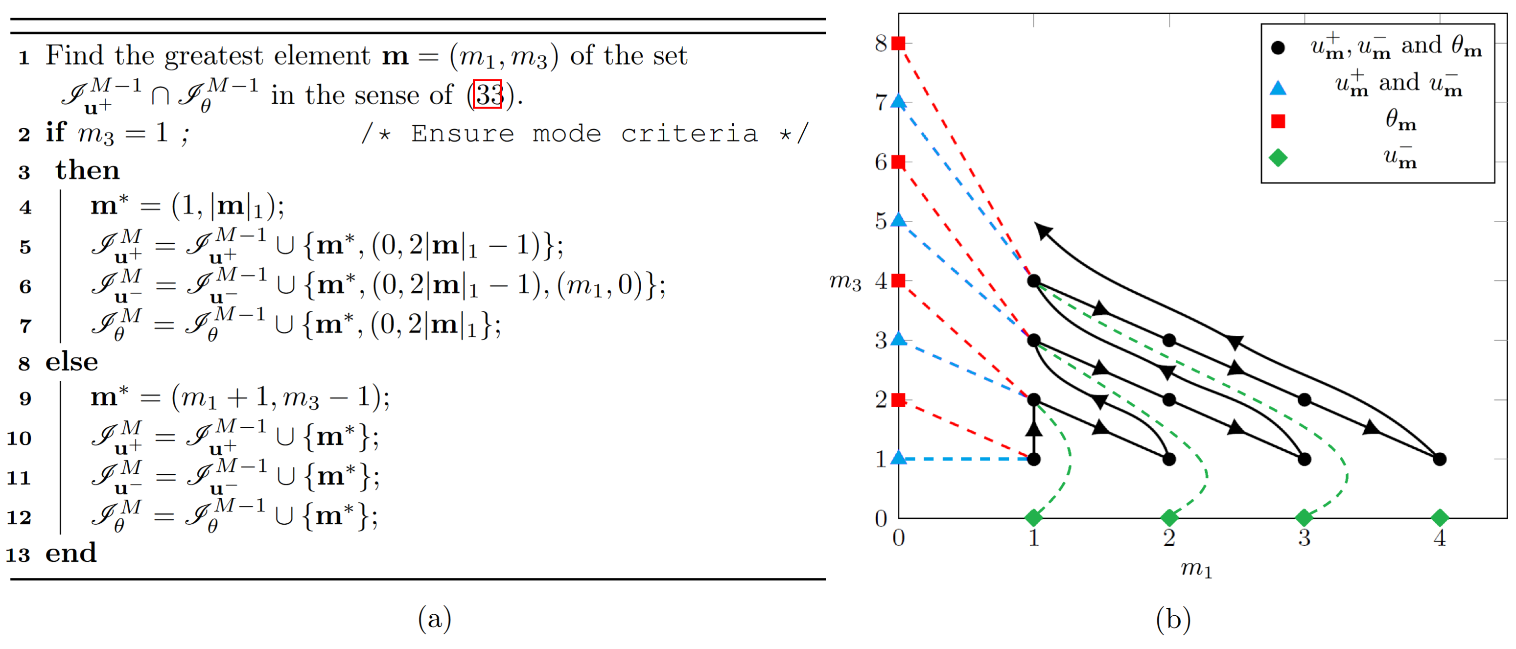
Figure 1. (a) The mode selection algorithm for the HKC hierarchy, (b) A depiction of the mode selection process, with shapes indicating which index sets $\mathscr{I}_{\textbf{u}^{\pm}}^{M},\mathscr{I}_{\theta}^{M}$ the modes are adjoined to, and the dashed lines indicated at which interior mode the shear modes $u^{\pm}_{(0,m_{3})},u^{-}_{(m_{1},0)}$ and stratified modes $\theta_{(0,m_{3})}$ are adjoined to ensure that Criteria 2.1 are satsified.

Due to relative simplicity of the lowest level model of this hierarchy, the HKC-1 model is given here explicitly:

(49) $$\begin{split}\frac{d}{dt}\theta_{(0,2)}&=-4\theta_{(0,2)}\hskip 192.05609pt+\frac{k_{1}}{\sqrt{2(k_{1}^{2}+1)}V}u_{(1,1)}^{+}\theta_{(1,1)}\\ \frac{d}{dt}u^{+}_{(1,1)}&=-\mathsf{P}(k_{1}^{2}+1)u^{+}_{(1,1)}-\frac{\mathsf{P}\mathcal{R}k_{1}}{\sqrt{k_{1}^{2}+1}}\theta_{(1,1)}+\frac{\mathsf{P}\mathscr{R}}{\sqrt{k_{1}^{2}+1}}u^{-}_{(1,1)}\\ \frac{d}{dt}u^{-}_{(1,1)}&=-\mathsf{P}(k_{1}^{2}+1)u^{-}_{(1,1)}\hskip 73.97733pt-\frac{\mathsf{P}\mathscr{R}}{\sqrt{k_{1}^{2}+1}}u^{+}_{(1,1)}\\ \frac{d}{dt}\theta_{(1,1)}&=-(k_{1}^{2}+1)\theta_{(1,1)}-\frac{k_{1}}{\sqrt{k_{1}^{2}+1}}u^{+}_{(1,1)}\hskip 86.78099pt-\frac{k_{1}}{\sqrt{2(k_{1}^{2}+1)}V}u_{(1,1)}^{+}\theta_{(0,2)}.\end{split}$$

together with the equations

$$\frac{d}{dt}u^{+}_{(0,1)}=-\mathsf{P}u^{+}_{(0,1)}+\mathsf{P}\mathscr{R}u^{-}_{(0,1)}\hskip 14.22636pt\text{ , }\frac{d}{dt}u^{-}_{(0,1)}=-\mathsf{P}u^{-}_{(0,1)}-\mathsf{P}\mathscr{R}u^{+}_{(0,1)}.$$

which are decoupled from the rest of the system and hence $u^{+}_{(0,1)},u^{-}_{(0,1)}$ decay exponentially. Note that this model is essentially the Lorenz-Stenflo model [24], aside from a linear change of variables and the trivial addition of $u^{+}_{(0,1)},u^{-}_{(0,1)}$.

In general, the $M$th model in the HKC hierarchy is a system of ODE of dimension

$$3M+4n-1\hskip 28.45274pt\text{ where }\hskip 28.45274ptn=\Big{\lfloor}\frac{\sqrt{8M+1}-1}{2}\Big{\rfloor}.$$

More specifically, the $M$th model contains $n$ vertically stratified temperature modes of the form $\theta_{(0,m_{3})}$, $n$ pairs of Coriolis coupled shear velocity modes of the form $\textbf{u}^{\pm}_{(0,m_{3})}$, $n-1$ transverse shear velocity modes of the form $\textbf{u}^{-}_{(m_{1},0)}$ and $M$ triples of Coriolis and buoyancy coupled modes $(\textbf{u}^{\pm}_{\textbf{m}},\theta_{\textbf{m}})$. Note that there is some ambiguity in when the $u_{(m_{1},0)}^{-}$ modes are included, since these do not enter into Criteria 2.1. In the HKC hierarchy, the choice to add the $u_{(m_{1},0)}^{-}$ modes beginning from HKC-2 was made so that the lowest order model is the Lorenz-Stenflo model, and time will tell whether this choice makes an impact.

Note the HKC models possess the following symmetries

(50) $$\begin{split}(u^{\pm}_{\textbf{m}})_{\textbf{m}\in\mathscr{I}_{\textbf{u}}^{M}}\text{ , }(\theta_{\textbf{m}})_{\textbf{m}\in\mathscr{I}_{\theta}^{M}}\hskip 14.22636pt\text{ is a solution }\hskip 14.22636pt&\text{ iff }\hskip 14.22636pt((-1)^{m_{1}}u^{\pm}_{\textbf{m}})_{\textbf{m}\in\mathscr{I}_{\textbf{u}}^{M}}\text{ , }((-1)^{m_{1}}\theta_{\textbf{m}})_{\textbf{m}\in\mathscr{I}_{\theta}^{M}}\hskip 14.22636pt\text{ is a solution}\\ \text{ iff }\hskip 14.22636pt((-1)^{m_{3}}u^{\pm}_{\textbf{m}})_{\textbf{m}\in\mathscr{I}_{\textbf{u}}^{M}}&\text{ , }((-1)^{m_{3}}\theta_{\textbf{m}})_{\textbf{m}\in\mathscr{I}_{\theta}^{M}}\hskip 14.22636pt\text{ is a solution.}\end{split}$$

While it is clear that the linear evolution is invariant under these symmetries, the nonlinear evolution is invariant as well since the index conditions $m_{1}=|p_{1}\pm q_{1}|$, $m_{3}=|p_{3}\pm q_{3}|$ must be satisfied.

Finally, in the context of the HKC models, one can define an analogous Nusselt number as follows:

$$\mathsf{Nu}^{M}=1+\frac{k_{1}}{2\pi^{3}}\overline{\langle u^{+,M}_{3}\theta^{M}\rangle}.$$

On the other hand, note that by taking the infinite time averages of the evolution equations in (6), one obtains the following equivalent expressions for the Nusselt number in terms of $\theta$:

$$\mathsf{Nu}=1+\frac{k_{1}}{2\pi^{3}}\overline{\langle u_{3}\theta\rangle}=1+\frac{k_{1}}{2\pi^{3}}\overline{\langle|\nabla\theta|^{2}\rangle}=1+\frac{k_{1}}{2\pi^{2}}\overline{\langle(1-\frac{x_{3}}{\pi})\partial_{x_{3}}^{2}\theta\rangle}.$$

These various expressions are useful in different contexts. For instance while the first has a clear physical interpretation as the average vertical heat transport, it is clear from the second that the Nusselt number must be greater than or equal to 1, i.e. a convective flow transports more heat than the pure conductive state. Since the same evolution equations hold for the HKC models, one has the analogous equivalent expressions. In the computational work below, the third expression will be most useful, since it expresses the Nusselt number in terms of the least number of modes, and furthermore finite time averages must be considered. Hence the finite time Nusselt number is defined via the third expression as follows:

(51) $$\mathsf{Nu}^{M}(t):=1-\sum_{\textbf{m}\in\mathscr{I}_{\theta}^{M}\cap\mathscr{I}^{*}}\frac{\sqrt{k_{1}}m_{3}}{\pi^{2}}\frac{1}{t}\int_{0}^{t}\theta_{\textbf{m}}^{M}(s)ds.$$

3. Existence of solutions and attractors

3.1. Well-posedness and attractor theory

Since the fluid is assumed to be horizontally aligned, the well-posedness theory for the model (8) is similar to that in the two-dimensional, non-rotating case. For example in [27], Temam provides a full proof of existence and uniqueness of solutions for the forced Navier-Stokes, although the Boussinesq equations are not considered. On the other hand in [26], Temam proves existence for a class of Navier-Stokes type equations, for which the Boussinesq equations are a particular case, although many details of the proof are omitted. However, Temam does not consider the case of free slip boundary conditions at both boundaries, nor three dimensional velocity fields nor the Coriolis force. The correspondence between the Galerkin truncation models and the full PDE is a major point of interest for this paper, hence a full proof of existence for (8) is given in this section. First, in following Lemma some classical inequalities are stated which will be used in the existence proof. For the first two inequalities, the main point is that these inequalities also hold for mean-zero functions, rather than just in the usual case of functions satisfying Dirichlet conditions. Since in the previous section an explicit basis has been given, these inequalities can be established by referring to the Fourier basis, hence the proofs are omitted. The last inequality is a version of the classical Gronwall inequality adapted to systems of inequalities (see for instance [2] for proof).

Lemma 3.1.

(a) (Poincaré) For $\textbf{u}\in\textbf{L}_{\sigma}^{2}$, $\theta\in L_{0}^{2}$ one has

(52) $$\|u_{3}\|_{L^{2}}\leq\|\nabla u_{3}\|_{L^{2}}\hskip 14.22636pt\text{ , }\hskip 14.22636pt\|\theta\|_{L^{2}}\leq\|\nabla\theta\|_{L^{2}}\hskip 14.22636pt\text{ , }\hskip 14.22636pt\|u_{i}\|_{L^{2}}\leq\frac{1}{\min(1,k_{1}^{2})}\|\nabla u_{i}\|_{L^{2}}\text{ for }i=1,2$$

(b) (Gagliardo-Nirenburg-Sobolev) Let $p\in[2,\infty)$ and $\sigma=\frac{p-2}{p}$. There exists a constant $C>0$ such that for any $u\in H^{1}$ having mean-zero one has

(53) $$\|u\|_{L^{p}}\leq C\|u\|_{L^{2}}^{1-\sigma}\|\nabla u\|_{L^{2}}^{\sigma}$$

(c) (Gronwall) Suppose $\textbf{v}(t),\textbf{a}(t)$ continuously map $t\in(0,\infty)$ into $\mathbb{R}^{d}$, $d\geq 1$ and $H(t)$ continuously maps $t\in(0,\infty)$ into the non-negative matrices. If one has

$$\textbf{v}(t)\leq\textbf{a}(t)+\int_{0}^{t}H(s)\textbf{v}(s)ds$$

where the inequalities hold componenent-wise, then one has

(54) $$\textbf{v}(t)\leq\textbf{a}(t)+\int_{0}^{t}\exp\big{[}\int_{s}^{t}H(z)dz\big{]}H(s)\textbf{a}(s)ds$$

The following theorem proves existence, uniqueness and regularity properties for (8). Furthermore statements about the long time behavior of the solutions are proven, culminating in the existence of a compact global attractor in $\textbf{L}^{2}_{\sigma}\times L^{2}_{0}$.

Theorem 1.

(a) Given admissible parameters $\mathfrak{P}$ and $\textbf{u}_{0},\theta_{0}\in\textbf{L}_{\sigma}^{2}\times L^{2}_{0}$, for any $\tau>0$ there exists a unique $(\textbf{u}(t),\theta(t))\in C([0,\tau];\textbf{L}^{2}_{\sigma}\times L_{0}^{2})\cap L^{2}([0,\tau];\textbf{H}^{1}_{\sigma}\times H_{0}^{1})$ such that $(\textbf{u}(0),\theta(0))=(\textbf{u}_{0},\theta_{0})$ which solves (8) for $t>0$. Thus the semi-group

(55) $$S(t)(\textbf{u}_{0},\theta_{0}):=(\textbf{u}(t),\theta(t))$$

is well defined. Furthermore, these solutions satisfy (41).

(b) If $\|\theta_{0}\|_{L^{\infty}}\leq\pi$ then

$$\|\theta(t)\|_{L^{\infty}}\leq\pi\text{ for a.e. }t>0$$

On the other hand, if $\|\theta_{0}\|_{L^{\infty}}\leq\pi$ if not assumed, then

$$\theta(t)=\bar{\theta}(t)+\tilde{\theta}(t)$$

where $\|\bar{\theta}(t)\|_{L^{\infty}}\leq\pi$ and

$$\|\tilde{\theta}(t)\|_{L^{2}}\leq C(1+\|\theta_{0}\|_{L^{2}})e^{-2t}$$

(c) There exists an absorbing ball in $\textbf{H}^{1}_{\sigma}\times H^{1}_{0}$ for the semi-group $S(t)$. This is a compact subset of $\textbf{L}^{2}_{\sigma}\times L^{2}_{0}$, hence $S(t)$ admits a compact global attractor $\mathcal{A}$.

Proof.

With $\textbf{u}_{0},\theta_{0}\in\textbf{L}_{\sigma}^{2}\times L^{2}_{0}$ chosen as above, let $\textbf{u}_{0}^{M},\theta_{0}^{M}$ denote their projection onto the modes defined by the $M$th index set in the hierarchy. Note that the Galerkin solutions must each satisfy

$$\begin{split}\frac{1}{2}\frac{d}{dt}\|\textbf{u}^{M}\|_{\textbf{L}^{2}}^{2}+\mathsf{P}\|\nabla\textbf{u}^{M}\|_{\textbf{L}^{2}}^{2}&=\langle u_{3}^{M}\theta^{M}\rangle\\ \frac{1}{2}\frac{d}{dt}\|\theta^{M}\|_{L^{2}}^{2}+\|\nabla\theta^{M}\|_{L^{2}}^{2}&=\langle u_{3}^{M}\theta^{M}\rangle\end{split}$$

hence integrating and applying Young’s inequality one obtains

(56) $$\begin{split}\frac{1}{2}\|\textbf{u}^{M}(t)\|_{\textbf{L}^{2}}^{2}+\mathsf{P}\int_{0}^{t}\|\nabla\textbf{u}^{M}(s)\|_{\textbf{L}^{2}}^{2}ds&\leq\frac{1}{2}\|\textbf{u}^{M}_{0}\|_{\textbf{L}^{2}}^{2}+\frac{\mathsf{P}\mathcal{R}}{2}\int_{0}^{t}\big{[}\|u_{3}^{M}(s)\|_{L^{2}}^{2}+\|\theta^{M}(s)\|_{L^{2}}^{2}\big{]}ds\\ \frac{1}{2}\|\theta^{M}(t)\|_{L^{2}}^{2}+\int_{0}^{t}\|\nabla\theta^{M}(s)\|_{L^{2}}^{2}ds&\leq\frac{1}{2}\|\theta^{M}_{0}\|_{L^{2}}^{2}+\frac{1}{2}\int_{0}^{t}\big{[}\|u_{3}^{M}(s)\|_{L^{2}}^{2}+\|\theta^{M}(s)\|_{L^{2}}^{2}\big{]}ds\end{split}$$

Considering only the first term on the left hand side of each equation above, Gronwall’s inequality (54) gives

$$\begin{pmatrix}\|\textbf{u}^{M}(t)\|_{\textbf{L}^{2}}^{2}\\ \|\theta^{M}(t)\|_{L^{2}}^{2}\end{pmatrix}\leq\exp\Big{[}\begin{pmatrix}\mathsf{P}\mathcal{R}&\mathsf{P}\mathcal{R}\\ 1&1\end{pmatrix}t\Big{]}\begin{pmatrix}\|\textbf{u}_{0}\|_{\textbf{L}^{2}}^{2}\\ \|\theta_{0}\|_{L^{2}}^{2}\end{pmatrix}$$

This bound is independent of $M$, hence for any $\tau>0$ all of the Galerkin solutions are uniformly bounded in $L^{\infty}([0,\tau];\textbf{L}^{2}_{\sigma}\times L^{2}_{0})$. Reinserting this into (56), one has a bound on the $L^{2}([0,\tau];\textbf{H}^{1}_{\sigma}\times H^{1}_{0})$ norm which is independent on $M$. From (14), one sees that for any $(\textbf{v},\phi)\in\textbf{H}^{1}_{\sigma}\times H_{0}^{1}$ one has

(57) $$\begin{split}\langle\frac{\partial\textbf{u}^{M}}{\partial t}\cdot\textbf{v}\rangle&=-\mathsf{P}\langle\nabla\textbf{u}^{M}:\nabla\mathbb{P}_{\textbf{u}}^{M}[\textbf{v}]\rangle+\mathsf{P}\mathcal{R}\langle\theta^{M}\hat{e}_{3}\cdot\mathbb{P}_{\textbf{u}}^{M}[\textbf{v}]\rangle-\mathsf{P}\mathscr{R}\langle(\hat{e}_{3}\times\textbf{u}^{M})\cdot\mathbb{P}_{\textbf{u}}^{M}[\textbf{v}]\rangle-\langle\mathbb{P}_{\textbf{u}}^{M}[\textbf{v}]\cdot(\textbf{u}^{M}\cdot\nabla\textbf{u}^{M})\rangle\\ \langle\frac{\partial\theta^{M}}{\partial t}\phi\rangle&=-\langle\nabla\theta^{M}\cdot\nabla\phi\rangle+\langle u^{M}_{3}\mathbb{P}_{\theta}^{M}[\phi]\rangle-\langle\mathbb{P}_{\theta}^{M}[\phi](\textbf{u}^{M}\cdot\nabla\theta^{M})\rangle\end{split}$$

Note that by integrating by parts, using Cauchy-Schwartz and (53) one obtains

(58) $$\begin{split}\big{|}\langle\mathbb{P}_{\textbf{u}}^{M}[\textbf{v}]\cdot(\textbf{u}^{M}\cdot\nabla\textbf{u}^{M})\rangle\big{|}&\leq\|\textbf{u}^{M}\|_{L^{4}}^{2}\|\nabla\textbf{v}\|_{L^{2}}\leq C\|\textbf{u}^{M}\|_{L^{2}}\|\nabla\textbf{u}^{M}\|_{L^{2}}\|\nabla\textbf{v}\|_{L^{2}}\\ \big{|}\langle\mathbb{P}_{\theta}^{M}[\phi](\textbf{u}^{M}\cdot\nabla\theta^{M})\rangle\big{|}&\leq\|\textbf{u}^{M}\|_{L^{4}}\|\theta^{M}\|_{L^{4}}\|\nabla\phi\|_{L^{2}}\leq C\|\textbf{u}^{M}\|_{L^{2}}^{1/2}\|\nabla\textbf{u}^{M}\|_{L^{2}}^{1/2}\|\theta^{M}\|_{L^{2}}^{1/2}\|\nabla\theta^{M}\|_{L^{2}}^{1/2}\|\nabla\phi\|_{L^{2}}\end{split}$$

One can then square both sides of (57), integrate over $[0,\tau]$, and bound all of the terms on the right hand side in terms of the $L^{\infty}([0,\tau];\textbf{L}^{2}_{\sigma}\times L^{2}_{0})$ and $L^{2}([0,\tau];\textbf{H}^{1}_{\sigma}\times H^{1}_{0})$ norms on $(\textbf{u}^{M}(t),\theta^{M}(t))$, using (58) for the nonlinear terms. One thus obtains a uniform bound for $(\partial_{t}\textbf{u}^{M},\partial_{t}\theta^{M})$ in the space $L^{2}([0,\tau];\textbf{H}^{-1}_{\sigma}\times H^{-1}_{0})$, hence by the Aubin-Lions lemma [23] the collection of Galerkin solutions is relatively compact in $L^{2}([0,\tau];\textbf{L}^{2}_{\sigma}\times L^{2}_{0})$. Thus a sub-sequence converges strongly to some $(\textbf{u}(t),\theta(t))$ in $L^{2}([0,\tau];\textbf{L}^{2}_{\sigma}\times L^{2}_{0})$.

In fact, the sub-sequential limits must belong to the more regular subspace $L^{\infty}([0,\tau];\textbf{L}^{2}_{\sigma}\times L^{2}_{0})\cap L^{2}([0,\tau];\textbf{H}^{1}_{\sigma}\times H^{1}_{0})$. Let $(\textbf{u}^{M_{k}},\theta^{M_{k}})$ be a sub-sequence which converges strongly to some $(\textbf{u}(t),\theta(t))$ in $L^{2}([0,\tau];\textbf{L}^{2}_{\sigma}\times L^{2}_{0})$. Since this sub-sequence is again uniformly bounded in $L^{\infty}([0,\tau];\textbf{L}^{2}_{\sigma}\times L^{2}_{0})$, it is relatively compact in the weak-* topology due to the Banach-Alaoglu theorem. Hence there must be some point $(\textbf{u}^{*}(t),\theta^{*}(t))\in L^{\infty}([0,\tau];\textbf{L}^{2}_{\sigma}\times L^{2}_{0})$ and a further sub-sequence such that for all $(\textbf{v}(t),\phi(t))\in L^{1}([0,\tau];\textbf{L}^{2}_{\sigma}\times L^{2}_{0})$ one has

$$\lim_{j\to\infty}\int_{0}^{\tau}\Big{\langle}\begin{pmatrix}\textbf{u}^{M_{k_{j}}}(t)-\textbf{u}^{*}(t)\\ \theta^{M_{k_{j}}}(t)-\theta^{*}(t)\end{pmatrix}\cdot\begin{pmatrix}\textbf{v}(t)\\ \phi(t)\end{pmatrix}\Big{\rangle}dt=0$$

In particular, using the strong convergence this implies that for all $(\textbf{v}(t),\phi(t))\in L^{2}([0,\tau];\textbf{L}^{2}_{\sigma}\times L^{2}_{0})$ one has

$$\lim_{j\to\infty}\int_{0}^{\tau}\Big{\langle}\begin{pmatrix}\textbf{u}(t)-\textbf{u}^{*}(t)\\ \theta(t)-\theta^{*}(t)\end{pmatrix}\cdot\begin{pmatrix}\textbf{v}(t)\\ \phi(t)\end{pmatrix}\Big{\rangle}dt=0$$

and hence these two elements are equal in $L^{2}([0,\tau];\textbf{L}^{2}_{\sigma}\times L^{2}_{0})$, ie $(\textbf{u}(t),\theta(t))$ belongs to the subspace $L^{\infty}([0,\tau];\textbf{L}^{2}_{\sigma}\times L^{2}_{0})$. Similarly, since this sub-sequence is uniformly bounded in $L^{2}([0,\tau];\textbf{H}^{1}_{\sigma}\times H^{1}_{0})$, it is relatively compact in its weak-* topology. However, since this is a Hilbert space this is the same as its weak topology, hence there must be some point $(\tilde{\textbf{u}}(t),\tilde{\theta}(t))\in L^{2}([0,\tau];\textbf{H}^{1}_{\sigma}\times H^{1}_{0})$, and a further sub-sequence such that for all $(\textbf{v}(t),\phi(t))\in L^{2}([0,\tau];\textbf{H}^{1}_{\sigma}\times H^{1}_{0})$ one has

$$\lim_{j\to\infty}\int_{0}^{\tau}\Big{\langle}\nabla\begin{pmatrix}\textbf{u}^{M_{k_{j}}}(t)-\tilde{\textbf{u}}(t)\\ \theta^{M_{k_{j}}}(t)-\tilde{\theta}(t)\end{pmatrix}:\nabla\begin{pmatrix}\textbf{v}(t)\\ \phi(t)\end{pmatrix}\Big{\rangle}dt=0$$

On the other hand, since $\Delta$ is an isometry between $H^{1}$ and $H^{-1}$ this implies that for all $(\textbf{v}(t),\phi(t))\in L^{2}([0,\tau];\textbf{H}^{-1}_{\sigma}\times H^{-1}_{0})$ one has

$$\lim_{j\to\infty}\int_{0}^{\tau}\Big{\langle}\begin{pmatrix}\textbf{u}^{M_{k_{j}}}(t)-\tilde{\textbf{u}}(t)\\ \theta^{M_{k_{j}}}(t)-\tilde{\theta}(t)\end{pmatrix}\cdot\begin{pmatrix}\textbf{v}(t)\\ \phi(t)\end{pmatrix}\Big{\rangle}dt=0$$

In particular, this implies that for for all $(\textbf{v}(t),\phi(t))\in L^{2}([0,\tau];\textbf{L}^{2}_{\sigma}\times L^{2}_{0})$ one has

$$\lim_{j\to\infty}\int_{0}^{\tau}\Big{\langle}\begin{pmatrix}\textbf{u}(t)-\tilde{\textbf{u}}(t)\\ \theta(t)-\tilde{\theta}(t)\end{pmatrix}\cdot\begin{pmatrix}\textbf{v}(t)\\ \phi(t)\end{pmatrix}\Big{\rangle}dt=0$$

so it follows $(\textbf{u}(t),\theta(t))\in L^{2}([0,\tau];\textbf{H}^{1}_{\sigma}\times H^{1}_{0})$.

Testing (14) with $(\textbf{v},\phi)\in\textbf{C}_{1}^{\infty}([0,\tau];\textbf{C}_{\sigma}^{\infty}\times C_{0}^{1})$ one can then use the respective strong, weak and weak-* convergence to show that (8) holds for any sub-sequential limit $(\textbf{u}(t),\theta(t))$, where $\partial_{t}\textbf{u}$ and $\partial_{t}\theta$ are the distributional derivatives in time. Since (8), and all of the terms on the right hand side have been shown to have certain regularity, it then becomes clear that the distributional derivatives $(\partial_{t}\textbf{u}(t),\partial_{t}\theta^{M}(t))$ belong to $L^{2}([0,\tau];\textbf{H}^{-1}_{\sigma}\times H_{0}^{-1})$, and using the Lions-Magenes lemma one can conclude that $(\textbf{u}(t),\theta(t))\in C([0,\tau];\textbf{L}^{2}_{\sigma}\times L^{2}_{0})$, and that

$$\frac{d}{dt}\|\textbf{u}\|_{\textbf{L}^{2}}^{2}=\langle\partial_{t}\textbf{u}(t),\textbf{u}(t)\rangle\hskip 14.22636pt\text{ , }\hskip 14.22636pt\frac{d}{dt}\|\theta\|_{L^{2}}^{2}=\langle\partial_{t}\theta(t),\theta(t)\rangle$$

holds in a distributional sense.

Having proven existence and regularity, one can show that the limit is unique. Suppose that $(\textbf{u}(t),\theta(t))$, $(\tilde{\textbf{u}}(t),\tilde{\theta}(t))$ are two different sub-sequential limits. The difference $(\textbf{w},\psi)=(\textbf{u}-\tilde{\textbf{u}},\theta-\tilde{\theta})$ must satisfy

$$\frac{1}{2}\frac{d}{dt}\Big{[}\|\textbf{w}\|_{\textbf{L}^{2}}^{2}+\|\psi\|_{\textbf{L}^{2}}^{2}\Big{]}+\mathsf{P}\|\textbf{w}\|_{\textbf{H}^{1}}^{2}+\|\psi\|_{\textbf{H}^{1}}^{2}=\text{ }\big{(}\mathsf{P}\mathcal{R}+1\big{)}\big{\langle}w_{3}\psi\big{\rangle}-\big{\langle}\textbf{w}\cdot\big{(}\textbf{u}\cdot\nabla\textbf{u}-\tilde{\textbf{u}}\cdot\nabla\tilde{\textbf{u}}\big{)}\big{\rangle}-\big{\langle}\psi\big{(}\textbf{u}\cdot\nabla\theta-\tilde{\textbf{u}}\cdot\nabla\tilde{\theta}\big{)}\big{\rangle}$$

Integrating over $[0,t]$, one can use

$$\begin{split}\textbf{u}\cdot\nabla\textbf{u}-\tilde{\textbf{u}}\cdot\nabla\tilde{\textbf{u}}=(\textbf{u}-\tilde{\textbf{u}})\cdot\nabla\textbf{u}+\tilde{\textbf{u}}\cdot\nabla(\textbf{u}-\tilde{\textbf{u}})\\ \textbf{u}\cdot\nabla\theta-\tilde{\textbf{u}}\cdot\nabla\tilde{\theta}=(\textbf{u}-\tilde{\textbf{u}})\cdot\nabla\theta+\tilde{\textbf{u}}\cdot\nabla(\theta-\tilde{\theta})\end{split}$$

and together with the Cauchy-Schwartz inequality, a bound similar to (58) and Young’s inequality, one obtains

$$\|\textbf{w}(t)\|_{\textbf{L}^{2}}^{2}+\|\psi(t)\|_{L^{2}}^{2}\leq\text{ }\int_{0}^{t}\Big{(}\big{(}\mathsf{P}\mathcal{R}+1+C(\frac{1}{\mathsf{P}^{3}}\|\textbf{u}\|_{\textbf{L}^{2}}^{2}\|\nabla\textbf{u}\|_{\textbf{L}^{2}}^{2}+\|\theta\|_{L^{2}}^{2}\|\nabla\theta\|_{L^{2}}^{2})\big{)}\|\textbf{w}(s)\|_{\textbf{L}^{2}}^{2}+\big{(}\mathsf{P}\mathcal{R}+1\big{)}\|\psi(s)\|_{L^{2}}^{2}\Big{)}ds$$

for a.e. $t\in[0,\tau]$. Using the bounds in $L^{\infty}([0,\tau];\textbf{L}_{\sigma}^{2}\times L_{0}^{2})$ and $L^{2}([0,\tau];\textbf{H}_{\sigma}^{1}\times H_{0}^{1})$ together with Gronwall’s inequality, one obtains

$$\|\textbf{u}(t)-\tilde{\textbf{u}}(t)\|_{\textbf{L}^{2}}^{2}+\|\theta(t)-\tilde{\theta}(t)\|_{\textbf{L}^{2}}^{2}=0\hskip 14.22636pt\text{ for a.e. }t\in[0,\tau]$$

hence the limit is unique.

Part (b) is the analogue of Temam’s Lemma 3.2 in Chapter 3 of [26], and the proof therein carries through identically for the present problem. To briefly recall, the proof is given in terms of the temperature $T$ in order to eliminate the additional $u_{3}$ term, since part (a) provides existence for $T$ with the same regularity as $\theta$, although with different boundary conditions. Set $\tilde{T}_{+}=\max(T-1,0)$, $\tilde{T}_{-}=\max(-T,0)$. By testing the temperature in (1) with $\tilde{T}_{+}$, one obtains

$$\frac{1}{2}\frac{d}{dt}\|\tilde{T}_{+}\|_{L^{2}}^{2}+\|\tilde{T}_{+}\|_{H^{1}}^{2}=0$$

and by the Poincaré inequality and Gronwall’s inequality one has

$$\|\tilde{T}_{+}(t)\|_{L^{2}}\leq\|\tilde{T}_{+}(0)\|_{L^{2}}e^{-2t}$$

for a constant $C$. The same reasoning applies to $\tilde{T}_{-}$, and taking $\tilde{T}=\tilde{T}_{+}-\tilde{T}_{-}$ is sufficient to prove (b).

Next, it is proven that the evolution defined by (8) admits an attracting, forward invariant ball in $H$. Using (b) one can prove that for any $\epsilon>0$ there exists $t^{*}(\epsilon)>0$ such that $\|\theta(t)\|_{L^{2}}\leq\sqrt{\pi|\Omega|}+\epsilon$ for all $t>t^{*}(\epsilon)$. One can therefore prove the velocity eventually enters a ball in $L^{2}$, where it remains ever after as follows. Testing the momentum equation with u, one obtains

(59) $$\begin{split}\frac{1}{2\mathsf{P}}\frac{d}{dt}\|\textbf{u}\|_{\textbf{L}^{2}}^{2}&=-\langle|\nabla\textbf{u}|^{2}\rangle+\mathcal{R}\langle u_{3}\theta\rangle\leq-\min(1,k_{1}^{2})\langle u_{1}^{2}+u_{2}^{2}\rangle-\langle u_{3}^{2}\rangle+\mathcal{R}\|\theta\|_{L^{2}}\|u_{3}\|_{L^{2}}\\ &\leq-\min(1,k_{1}^{2})\langle u_{1}^{2}+u_{2}^{2}\rangle-\langle u_{3}^{2}\rangle+\mathcal{R}(\sqrt{\pi|\Omega|}+\epsilon)\|u_{3}\|_{L^{2}}\\ &\leq-\min(1,k_{1}^{2})\langle u_{1}^{2}+u_{2}^{2}\rangle-\big{(}\|u_{3}\|_{L^{2}}-\frac{1}{2}\mathcal{R}(\sqrt{\pi|\Omega|}+\epsilon)\big{)}^{2}+\frac{\mathcal{R}^{2}(\sqrt{\pi|\Omega|}+\epsilon)^{2}}{4}.\end{split}$$

Thus the radius of $(\|u_{1}\|_{L^{2}},\|u_{2}\|_{L^{2}},\|u_{3}\|_{L^{2}})$ decreases unless the norms of the solution lie in the ellipsoid centered at $(\|u_{1}\|_{L^{2}},\|u_{2}\|_{L^{2}},\|u_{3}\|_{L^{2}})=(0,0,\frac{1}{2}\mathcal{R}(\sqrt{\pi|\Omega|}+\epsilon))$. Therefore any larger ball centered at the origin containing this ellipsoid in its interior is an attracting, forward invariant set, for instance the ball $B(0,\mathcal{R}(\sqrt{\pi|\Omega|}+2\epsilon))$

Finally, one can bootstrap the result to prove the evolution defined by (8) admits an attracting, forward invariant ball in $V$. First, by integrating the equations for the $L^{2}$ norms from time $t$ to $t+1$, one obtains

$$\begin{split}\frac{1}{2\mathsf{P}}\big{(}\|\textbf{u}(t+1)\|_{\textbf{L}^{2}}^{2}-\|\textbf{u}(t)\|_{\textbf{L}^{2}}^{2}\big{)}&=-\int_{t}^{t+1}\|\nabla\textbf{u}(s)\|_{\textbf{L}^{2}}^{2}ds+\mathcal{R}\int_{t}^{t+1}\langle u_{3}(s)\theta(s)\rangle ds\\ \frac{1}{2}\big{(}\|\theta(t+1)\|_{L^{2}}^{2}-\|\theta(t)\|_{L^{2}}^{2}\big{)}&=-\int_{t}^{t+1}\|\nabla\theta(s)\|_{L^{2}}^{2}ds+\int_{t}^{t+1}\langle u_{3}(s)\theta(s)\rangle ds\end{split}$$

hence for $t>t^{*}(\epsilon)$ one can use Cauchy-Schwarz, Young’s inequality and the bounds on the $L^{2}$ norms of $\textbf{u},\theta$ to obtain

(60) $$\begin{split}\int_{t}^{t+1}\|\nabla\textbf{u}(s)\|_{\textbf{L}^{2}}^{2}ds&\leq\frac{\mathcal{R}}{2}(\mathcal{R}+1+\frac{2}{\mathsf{P}})(\sqrt{\pi|\Omega|}+2\epsilon)\\ \int_{t}^{t+1}\|\nabla\theta(s)\|_{L^{2}}^{2}ds&\leq\frac{1}{2}(\mathcal{R}+3)(\sqrt{\pi|\Omega|}+2\epsilon)\end{split}$$

Next, by testing the momentum equation with $-\Delta\textbf{u}$, then using Cauchy-Scwarz, Poincaré and Young’s inequalities together with taking $\textbf{v}=\Delta\textbf{u}$ in (58), one obtains

$$\begin{split}\frac{1}{2\mathsf{P}}\frac{d}{dt}\|\nabla\textbf{u}\|_{\textbf{L}^{2}}^{2}&=-\|\Delta\textbf{u}\|_{L^{2}}^{2}+\frac{1}{\mathsf{P}}\langle\big{(}(\textbf{u}\cdot\nabla)\textbf{u}\big{)}\cdot\Delta\textbf{u}\rangle+\mathcal{R}\langle\nabla u_{3}\cdot\nabla\theta\rangle\\ &\leq-\|\Delta\textbf{u}\|_{L^{2}}^{2}+\frac{1}{\mathsf{P}}\|(\textbf{u}\cdot\nabla)\textbf{u}\|_{L^{2}}\|\Delta\textbf{u}\|_{L^{2}}+\mathcal{R}\|\nabla u_{3}\|_{L^{2}}\|\nabla\theta\|_{L^{2}}\\ &\leq-\frac{1}{2}\|\Delta\textbf{u}\|_{L^{2}}^{2}+\frac{1}{\mathsf{P}}\|\textbf{u}\|_{L^{2}}^{1/2}\|\nabla\textbf{u}\|_{L^{2}}\|\Delta\textbf{u}\|_{L^{2}}^{3/2}+\frac{\mathcal{R}^{2}}{2\min(1,k_{1}^{4})}\|\nabla\theta\|_{L^{2}}^{2}\\ &\leq-\frac{1}{4}\|\Delta\textbf{u}\|_{L^{2}}^{2}+\frac{27}{4\mathsf{P}^{4}}\|\textbf{u}\|_{L^{2}}^{2}\|\nabla\textbf{u}\|_{L^{2}}^{4}+\frac{\mathcal{R}^{2}}{2\min(1,k_{1}^{4})}\|\nabla\theta\|_{L^{2}}^{2}\end{split}$$

Hence one has

$$\frac{d}{dt}\|\nabla\textbf{u}\|_{\textbf{L}^{2}}^{2}\leq\Big{(}\frac{27}{2\mathsf{P}^{3}}\|\textbf{u}\|_{L^{2}}^{2}\|\nabla\textbf{u}\|_{L^{2}}^{2}\Big{)}\|\nabla\textbf{u}\|_{L^{2}}^{2}+\frac{\mathsf{P}\mathcal{R}^{2}}{\min(1,k_{1}^{4})}\|\nabla\theta\|_{L^{2}}^{2}$$

and together with (60) it follows from the Gronwall inequality, that for $t>t^{*}(\epsilon)+1$ one has

$$\|\nabla\textbf{u}(t)\|_{\textbf{L}^{2}}^{2}\leq\big{(}\frac{\mathsf{P}\mathcal{R}^{2}(\mathcal{R}+3)}{2\min(1,k_{1}^{4})}+\frac{\mathcal{R}}{2}(\mathcal{R}+1+\frac{2}{\mathsf{P}})\big{)}(\sqrt{\pi|\Omega|}+2\epsilon)\exp\Big{[}\frac{27\mathcal{R}^{3}}{4\mathsf{P}^{3}}(\pi|\Omega|+2\epsilon)^{3}(\mathcal{R}+1+\frac{2}{\mathsf{P}})\Big{]}.$$

The same argument can be used to obtain a bound on $\|\nabla\theta\|_{L^{2}}^{2}$, thus proving the result.

Finally, letting $B$ denote the attracting ball, the proof $\mathcal{A}=\omega(B)$ has the properties of the global attractor is the same as in the finite dimensional case above. ∎

Remark 3.2.

To illustrate the power of the balance relations (41) for characterizing the behavior of solutions of the PDE, note that these alone are sufficient to characterize the global attractor in the case of small Rayleigh number. Adding the kinetic energy and $\theta^{2}$ equations and using the Poincare inequalities one obtains:

$$\frac{1}{2}\frac{d}{dt}\big{[}\langle|\textbf{u}|^{2}\rangle+\langle\theta^{2}\rangle\big{]}=-\mathsf{P}\langle|\nabla\textbf{u}|^{2}\rangle+(\mathsf{P}\mathcal{R}+1)\langle u_{3}\theta\rangle-\langle|\nabla\theta|^{2}\rangle\leq-\mathsf{P}\min(1,k_{1}^{2})\langle u_{1}^{2}+u_{2}^{2}\rangle-\mathsf{P}\langle u_{3}^{2}\rangle+(\mathsf{P}\mathcal{R}+1)\langle u_{3}\theta\rangle-\langle\theta^{2}\rangle.$$

The last terms on the right hand side can be expressed as follows

$$-\mathsf{P}\langle u_{3}^{2}\rangle+(\mathsf{P}\mathcal{R}+1)\langle u_{3}\theta\rangle-\langle\theta^{2}\rangle=\langle\begin{pmatrix}u_{3}\\ \theta\end{pmatrix}\begin{pmatrix}-\mathsf{P}&\frac{\mathsf{P}\mathcal{R}+1}{2}\\ \frac{\mathsf{P}\mathcal{R}+1}{2}&-1\end{pmatrix}\begin{pmatrix}u_{3}\\ \theta\end{pmatrix}\rangle,$$

hence the right hand side is an inner product with a negative semi-definite matrix until a critical Rayleigh number $\mathcal{R}_{0,glob}:=\frac{2}{\sqrt{\mathsf{P}}}-\frac{1}{\mathsf{P}}$. $\mathcal{R}_{0,glob}$ is strictly positive for $\mathsf{P}>\frac{1}{4}$ which are the values of the Prandtl number considered in this paper. Hence for $0\leq\mathcal{R}<\mathcal{R}_{0,glob}$ the total energy is a Lyapunov function for (8) and the origin is the global attractor. However, this is a conservative estimate and does not necessarily indicate when the global attractor develops further structure.

4. The dimension of the attractor and an analysis of bifurcations

As the above proof of Theorem 1 has shown, one has the convergence result that for any $\tau>0$ and any $\epsilon>0$ there exists a $M^{*}(\tau,\epsilon)>0$ such that for all $M>M^{*}(\tau,\epsilon)$ one has

(61) $$\int_{0}^{\tau}\int_{\Omega}\Big{[}|\textbf{u}(x,t)-\textbf{u}^{M}(x,t)|^{2}+|\theta(x,t)-\theta^{M}(x,t)|^{2}\Big{]}dxdt<\epsilon.$$

For such a Galerkin approximation one has

$$\big{|}\frac{1}{\tau}\int_{0}^{\tau}\int_{\Omega}\big{[}u_{3}\theta-u_{3}^{M}\theta^{M}\big{]}dxdt\big{|}\leq\frac{1}{\tau^{1/2}}\int_{0}^{\tau}\Big{[}\|\theta\|_{L^{2}}^{2}\|u_{3}-u_{3}^{M}\|_{L^{2}}^{2}+\|u_{3}^{M}\|_{L^{2}}^{2}\|\theta-\theta^{M}\|_{L^{2}}^{2}\Big{]}<\frac{C\epsilon}{\tau^{1/2}},$$

where the constant $C$ depends only on the initial condition and the radii of the absorbing balls described above. However, the above proof does not provide a rate of convergence, hence even for finite time averages the number of necessary modes $M^{*}(\tau,\epsilon)$ is unknown. Furthermore, it is unclear whether the above result about finite time approximation is sufficient for an infinite time average such as the Nusselt number. Indeed, as for the classical Lorenz model one expects to see exponential divergence of nearby trajectories, hence it is plausible that $M^{*}(\tau,\epsilon)\to\infty$ as $\tau\to\infty$.

This section therefore aims at studying the properties of the global attractor in order to provide a stronger theoretical basis for the numerical heat transport analysis in section 5. First, Temam’s result on the Hausdorff dimension of the attractor is restated, which provides a bound on the complexity of the attractor as a function of the Rayleigh number. It is difficult to discern whether this bound is sharp, and the due to computational burden imposed by the large Rayleigh numbers involved in atmosphere flows it is essential to have sharpest available bound. The unstable manifold of the origin is a component of the attractor about which analytical statements can be made, hence the local bifurcations at the origin are studied to provide a lower bound on the dimension of the attractor.

4.1. Upper bound on the attractor dimension for the Boussinesq Coriolis model

Recall that the $d$-dimensional Hausdorff measure of $\mathcal{A}$ is the number

$$\mu_{H}(\mathcal{A},d):=\sup_{\epsilon>0}\inf_{C\in\mathcal{C}_{\epsilon}}\sum\nolimits_{i=1}^{|C|}r_{i}^{d},$$

where $\mathcal{C}_{\epsilon}$ is the collection of all coverings $C$ of $\mathcal{A}$ by balls $B_{i}$ of radius $0<r_{i}\leq\epsilon$. The Hausdorff dimension of $\mathcal{A}$, $d_{Haus}(\mathcal{A})$, is defined as the unique number such that for all $d\in[0,\infty)$ one has $\mu_{H}(\mathcal{A},d)=0$ if $d>d_{Haus}(\mathcal{A})$ and $\mu_{H}(\mathcal{A},d)=\infty$ if $d<d_{Haus}(\mathcal{A})$. On the other hand the box-counting dimension of $\mathcal{A}$ is defined

$$d_{box}(\mathcal{A}):=\limsup_{\epsilon\to 0}\frac{\log n_{\mathcal{A}}(\epsilon)}{\log 1/\epsilon},$$

where $n_{\mathcal{A}}(\epsilon)$ is the number of balls of radius $\leq\epsilon$ which is necessary to cover $\mathcal{A}$. Note that Temam refers to the box-counting dimension as the fractal dimension, whereas nowadays the term fractal dimension is used more generally to refer to any index which characterizes fractal sets by quantifying their complexity.

Temam’s result is for non-rotating, planar flows, hence $\mathscr{R}=0$, and $u_{2}(\textbf{x},t)=0$ for all $t\geq 0$. For $\mathscr{R}=0$, the condition $u_{2}(\textbf{x},t)=0$ is invariant for the flow defined by (1), hence in the notation of this paper the result can be stated as follows:

Theorem 2 (Foias, Manley, Temam [10] Theorem 5.1).

Suppose $\mathscr{R}=0$, $u_{2,0}(\textbf{x})=0$ and let $\mathcal{A}$ be the global attractor of $S(t)$ defined in (55). There exists constants $C_{Haus},C_{box}$ depending only on $\mathsf{P},k_{1}$ such that one has the following bounds

(62) $$d_{Haus}(\mathcal{A})\leq C_{Haus}(1+\mathcal{R})\hskip 14.22636pt\text{ , }\hskip 14.22636ptd_{box}(\mathcal{A})\leq C_{box}(1+\mathcal{R}).$$

In fact, one can check that this result carries over to the general case $\mathscr{R}\geq 0$, $u_{2,0}(\textbf{x})\neq 0$, with different constants $\tilde{C}_{Haus},\tilde{C}_{box}$. Hence (62) is used in the analysis in section 5 with $\tilde{C}_{Haus}$. The proof for the general case is so similar to that in [10] that it is not repeated here in full detail. However, by carefully analyzing the proof, one can extract the constant $\tilde{C}_{Haus}$, hence a sketch of the proof is provided to show how these arise. The result is as follows:

(63) $$\tilde{C}_{Haus}=\frac{320\pi^{3}}{\mathsf{P}(1+\mathsf{P})\min(1,k_{1}^{2})}.$$

The crux of the proof studies how $d$-dimensional infinitesimal volumes are expanded or contracted by the flow, for arbitrary $d>0$. The goal is to find an $d$ large enough such that all higher dimensional infinitesimal volumes are contracted by the flow, and by appealing to a more general theorem on the relation between the Lyapunov exponents and the Hausdorff dimension (see [26] Theorem V.3.3), one concludes that the Hausdorff dimension is bounded by such an $d$. In order to study the distortion of infinitesimal volumes by the flow, one considers solutions of the linearization about the flow along the attractor. Namely for $j=1,...,d$, let $(\textbf{w}^{j}(t),\psi^{j}(t))$ solve

(64) $$\begin{split}\partial_{t}\textbf{w}^{j}&=\mathsf{P}\Delta\textbf{w}^{j}+\mathsf{P}\mathcal{R}\mathbb{P}\big{[}\psi^{j}\hat{e}_{3}\big{]}-\mathsf{P}\mathscr{R}\mathbb{P}\big{[}\hat{e}_{3}\times\textbf{w}^{j}\big{]}-\mathbb{P}\big{[}\textbf{u}\cdot\nabla\textbf{w}^{j}+\textbf{w}^{j}\cdot\nabla\textbf{u}\big{]}\\ \partial_{t}\psi^{j}&=\Delta\psi^{j}+w_{3}^{j}-\textbf{u}\cdot\nabla\psi^{j}-\textbf{w}^{j}\cdot\nabla\theta,\end{split}$$

for initial conditions $(\textbf{w}^{j}_{0},\psi^{j}_{0})$, in which $(\textbf{u}(t),\theta(t))$ is the solution from Theorem 1 corresponding to the initial condition $(\textbf{u}_{0},\theta_{0})\in\mathcal{A}$. Letting C be the matrix such that $\hat{e}_{3}\times\textbf{u}=\textbf{C}\textbf{u}$ and defining $\mathscr{L}_{Cori}=\mathbb{P}\textbf{C}$, (64) can be written as

(65) $$\frac{d}{dt}\begin{pmatrix}\textbf{w}^{j}(t)\\ \psi^{j}(t)\end{pmatrix}=L_{(\textbf{u}_{0},\theta_{0})}(t)\begin{pmatrix}\textbf{w}^{j}(t)\\ \psi^{j}(t)\end{pmatrix}\hskip 7.11317pt\text{ , }\hskip 7.11317ptL_{(\textbf{u}_{0},\theta_{0})}(t):=\begin{pmatrix}\mathsf{P}\Delta-\mathsf{P}\mathscr{R}\mathscr{L}_{Cori}-\mathbb{P}\big{[}\textbf{u}\cdot\nabla+(\nabla\textbf{u})^{T}\big{]}&\mathsf{P}\mathcal{R}\mathbb{P}\hat{e}_{3}^{T}\\ \hat{e}_{3}^{T}-(\nabla\theta)^{T}&\Delta-\textbf{u}\cdot\nabla\end{pmatrix}.$$

The $m$-dimensional volume of the parallelepiped formed by these vectors is given by the norm of the wedge product:

$$\Big{|}\begin{pmatrix}\textbf{w}^{1}\\ \psi^{1}\end{pmatrix}\wedge...\wedge\begin{pmatrix}\textbf{w}^{d}\\ \psi^{d}\end{pmatrix}\Big{|}_{\bigwedge^{d}\textbf{L}_{\sigma}^{2}\times L^{2}_{0}}^{2}:=\mathsf{det}\Big{(}\big{\langle}\begin{pmatrix}\textbf{w}^{i}\\ \psi^{i}\end{pmatrix}\cdot\begin{pmatrix}\textbf{w}^{j}\\ \psi^{j}\end{pmatrix}\big{\rangle}\Big{)}_{i,j=1}^{d}.$$

It can be shown (for instance [26] Lemma V.1.2) that one has

$$\Big{|}\begin{pmatrix}\textbf{w}^{1}(t)\\ \psi^{1}(t)\end{pmatrix}\wedge...\wedge\begin{pmatrix}\textbf{w}^{d}(t)\\ \psi^{d}(t)\end{pmatrix}\Big{|}_{\bigwedge^{d}\textbf{L}_{\sigma}^{2}\times L_{0}^{2}}=\Big{|}\begin{pmatrix}\textbf{w}^{1}_{0}\\ \psi^{1}_{0}\end{pmatrix}\wedge...\wedge\begin{pmatrix}\textbf{w}^{d}_{0}\\ \psi^{d}_{0}\end{pmatrix}\Big{|}_{\bigwedge^{d}\textbf{L}_{\sigma}^{2}\times L_{0}^{2}}\exp\Big{[}\int_{0}^{t}\mathsf{Tr}\Big{[}L_{(\textbf{u}_{0},\theta_{0})}(\tau)\circ Q_{d}(\tau)\Big{]}d\tau\Big{]},$$

where $Q_{d}(t)$ is the orthogonal projector of $\mathbb{L}^{2}_{\sigma}\times L^{2}_{0}$ onto the subspace spanned by $(\textbf{w}^{j}(t),\psi^{j}(t))$, $i=1,...,d$. Letting $(\textbf{v}^{j},\phi^{j})$, $j=1,...,d$ be orthonormal vectors spanning this same subspace, one has from the definition of $L_{(\textbf{u}_{0},\theta_{0})}(\tau)$

$$\begin{split}\mathsf{Tr}\Big{[}L_{(\textbf{u}_{0},\theta_{0})}(\tau)\circ Q_{d}(\tau)\Big{]}&=\sum_{j=1}^{d}\Big{\langle}\begin{pmatrix}\textbf{v}^{j}(\tau)\\ \phi^{j}(\tau)\end{pmatrix}\cdot L_{(\textbf{u}_{0},\theta_{0})}(\tau)\begin{pmatrix}\textbf{v}^{j}(\tau)\\ \phi^{j}(\tau)\end{pmatrix}\Big{\rangle}\\ &=\sum_{j=1}^{d}-\mathsf{P}\|\textbf{v}^{j}\|_{\textbf{H}^{1}}^{2}-\|\phi^{j}\|_{H^{1}}^{2}+(\mathsf{P}\mathcal{R}+1)\big{\langle}\phi^{j}v^{j}_{3}\big{\rangle}-\big{\langle}\phi^{j}\big{(}\textbf{v}^{j}\cdot\nabla\theta\big{)}+\textbf{v}^{j}\cdot\big{[}\textbf{v}^{j}\cdot\nabla\textbf{u}\big{]}\big{\rangle}.\end{split}$$

The first two sign indefinite terms are easily bounded as follows using Cauchy-Schwarz, the maximum principle $|\theta(\tau)|\leq\pi$, Young’s inequality, and the fact that $(\textbf{v}^{j},\psi^{j})$ are normalized:

$$\begin{split}&\big{|}\langle\phi^{j}\big{(}\textbf{v}^{j}\cdot\nabla\theta\big{)}\rangle\big{|}=\big{|}\langle\theta\big{(}\textbf{v}^{j}\cdot\nabla\phi^{j}\big{)}\rangle\big{|}\leq\pi\|\textbf{v}^{j}\|_{\textbf{L}^{2}_{\sigma}}\|\phi^{j}\|_{H^{1}}\leq\pi\|\phi^{j}\|_{H^{1}}\leq\frac{1}{2}\big{(}\pi^{2}+\|\phi^{j}\|_{H^{1}}^{2}\big{)}\\ &\big{\langle}\phi^{j}v^{j}_{3}\big{\rangle}\leq\frac{1}{2}\big{(}\|v^{j}_{3}\|_{L^{2}}^{2}+\|\phi^{j}\|_{L^{2}}^{2}\big{)}\leq\frac{1}{2}.\end{split}$$

The last term sign indefinite term is more difficult to bound, and requires use of the Sobolev-Lieb-Thirring inequality, which in this case states

(66) $$\|\sum_{j=1}^{d}(\textbf{v}^{j})^{2}\|_{\textbf{L}^{2}_{\sigma}}\leq\kappa_{1}\sum_{j=1}^{d}\|\textbf{v}^{j}\|_{\textbf{H}^{1}_{\sigma}},$$

for a constant $\kappa_{1}$ depending only on the domain $\Omega$. Hence one obtains

$$\big{|}\sum_{j=1}^{d}\langle\textbf{v}^{j}\big{(}\textbf{v}^{j}\cdot\nabla\textbf{u}\big{)}\rangle\big{|}\leq\|\textbf{u}\|_{\textbf{H}^{1}_{\sigma}}\|\sum_{j=1}^{d}(\textbf{v}^{j})^{2}\|_{\textbf{L}^{2}_{\sigma}}\leq\frac{1}{2}\big{(}\frac{\kappa_{1}^{2}}{\mathsf{P}}\|\textbf{u}\|_{\textbf{H}^{1}_{\sigma}}^{2}+\mathsf{P}\sum_{j=1}^{d}\|\textbf{v}^{j}\|_{\textbf{H}^{1}_{\sigma}}^{2}\big{)}.$$

Putting all of these equations together, one obtains

$$\mathsf{Tr}\Big{[}L_{(\textbf{u}_{0},\theta_{0})}(\tau)\circ Q_{d}(\tau)\Big{]}\leq\frac{\pi^{2}+1}{2}d+\frac{\kappa_{1}^{2}}{2\mathsf{P}}\|\textbf{u}\|_{\textbf{H}^{1}_{\sigma}}^{2}-\frac{1}{2}\sum_{j=1}^{d}\mathsf{P}\|\textbf{v}^{j}\|_{\textbf{H}^{1}}^{2}+\|\phi^{j}\|_{H^{1}}^{2}.$$

The fact that $(\textbf{v}^{j}$, $\theta^{j})$ are mutually orthogonal puts constraints on their Fourier expansions, and hence the following sum is bounded below by choosing $(\textbf{v}^{j}$, $\theta^{j})$ to have the $d$ lowest allowed wavenumbers $(m_{1},m_{3})$. The $H^{1}$ norms give a factor $m_{1}^{2}+m_{3}^{2}$, but since there are $n+1$ wavenumbers with $m_{1}+m_{3}=n$, the sum behaves as a sum over $j$:

$$\sum_{j=1}^{d}\mathsf{P}\|\textbf{v}^{j}\|_{\textbf{H}^{1}}^{2}+\|\phi^{j}\|_{H^{1}}^{2}\geq\sum_{j=1}^{d}(1+\mathsf{P})\mathsf{min}(1,k_{1}^{2})j\geq(1+\mathsf{P})\mathsf{min}(1,k_{1}^{2})\frac{d(d+1)}{2}.$$

Finally, since (60) applies for all time for initial conditions on the attractor, one obtains

$$\int_{0}^{t}\mathsf{Tr}\Big{[}L_{(\textbf{u}_{0},\theta_{0})}(\tau)\circ Q_{d}(\tau)\Big{]}d\tau\leq\Big{(}-\frac{(1+\mathsf{P})\mathsf{min}(1,k_{1}^{2})}{4}d(d+1)+\frac{\pi^{2}+1}{2}d+\frac{\kappa_{1}^{2}}{2\mathsf{P}}\frac{\mathcal{R}}{2}(\mathcal{R}+1+\frac{2}{\mathsf{P}})(\sqrt{\pi|\Omega|}+2\epsilon)\Big{)}t.$$

This is quadratic in $d$, with leading coefficient negative, hence one can solve for the $d$ such that all higher dimensional volumes are contracted. By gathering together the constants in this argument, one arrives at (63).

Remark 4.1.

Note that while (62) is independent of the rotation number, this bound is not necessarily sharp. Indeed, the analysis of the local bifurcations at the origin and the numerical work in section 5 strongly suggest that the rotation plays a significant role. However, a rotation dependent bound ended up being too difficult to prove for the present work. The main difficult is that the rotation is energy neutral and hence doesn’t enter into (60), hence one must use new methods. This will be discussed a bit further in the conclusion section.

Remark 4.2.

Note also that the constant $\kappa_{1}$ in the Lieb-Thirring inequality (66) can be taken to be

$$\kappa_{1}=\frac{4\pi^{2}}{\mathsf{min}(1,k_{1})}\inf_{1<k<2}2^{k}\int_{0}^{\infty}\frac{ds}{(1+s)^{k}}\int_{0}^{1}\rho^{1-k}(1-\rho)^{k}d\rho.$$

This can be extracted by following the arguments in the Appendix of [26], although in these arguments there is a confusing notational choice, perhaps a typo. Specifically, in the proof of the Birman-Schwinger inequality (Proposition 2.1) the exponent $k\geq 1$ is not the same $k$ which arises in the definition of the operator $\mathfrak{A}$ in (1.1).

4.2. Local bifurcations at the origin and a lower bound on the attractor dimension

For convenience, group the vertically stratified temperature modes $\theta_{(0,m_{3})}$, the pairs of Coriolis coupled shear velocity modes $\textbf{u}^{\pm}_{(0,m_{3})}$, the transverse shear velocity modes $\textbf{u}^{-}_{(m_{1},0)}$ and the triples of Coriolis and buoyancy coupled modes $(\textbf{u}^{\pm}_{\textbf{m}},\theta_{\textbf{m}})$ together into the vector z as follows:

$$\textbf{a}=\begin{pmatrix}\theta_{(0,2)}\\ \vdots\end{pmatrix}\hskip 7.11317pt\text{ , }\hskip 7.11317pt\textbf{b}=\begin{pmatrix}u^{+}_{(0,1)}\\ u^{-}_{(0,1)}\\ \vdots\end{pmatrix}\hskip 7.11317pt\text{ , }\hskip 7.11317pt\textbf{c}=\begin{pmatrix}u^{-}_{(1,0)}\\ \vdots\end{pmatrix}\hskip 7.11317pt\text{ , }\hskip 7.11317pt\textbf{f}=\begin{pmatrix}u^{+}_{(1,1)}\\ u^{-}_{(1,1)}\\ \theta_{(1,1)}\\ \vdots\end{pmatrix}\hskip 7.11317pt\text{ , }\hskip 7.11317pt\textbf{z}=\begin{pmatrix}\textbf{a}\\ \textbf{b}\\ \textbf{c}\\ \textbf{f}\end{pmatrix}.$$

The linearization of (8) about the origin can then be written as $\frac{d\textbf{z}}{dt}=\textbf{L}\textbf{z}$, where the operator $\textbf{L}=\mathsf{diag}(\textbf{A},\textbf{B},\textbf{C},\textbf{F})$ is block diagonal with block elements $\textbf{A},\textbf{C}$ only consisting of elements $-m_{3}^{2}$, $-k_{1}^{2}m_{1}^{2}$ along their diagonals, and where the block elements $\textbf{B},\textbf{F}$ are themselves block diagonal with sub-matrices given by

$$B^{\textbf{m}}=\begin{pmatrix}-\mathsf{P}|\textbf{Km}|^{2}&\mathsf{P}\mathscr{R}\\ -\mathsf{P}\mathscr{R}&-\mathsf{P}|\textbf{Km}|^{2}\end{pmatrix}\hskip 14.22636pt\text{ , }\hskip 14.22636ptF^{\textbf{m}}=\begin{pmatrix}-\mathsf{P}|\textbf{Km}|^{2}&\mathsf{P}\mathscr{R}\frac{m_{3}}{|\textbf{Km}|}&(-1)^{|\textbf{m}|_{1}+1}\mathsf{P}\mathcal{R}\frac{k_{1}m_{1}}{|\textbf{Km}|}\\ -\mathsf{P}\mathscr{R}\frac{m_{3}}{|\textbf{Km}|}&-\mathsf{P}|\textbf{Km}|^{2}&0\\ (-1)^{|\textbf{m}|_{1}+1}\frac{k_{1}m_{1}}{|\textbf{Km}|}&0&-|\textbf{Km}|^{2}\end{pmatrix}.$$

The spectrum of the linearization about the origin is studied in the following lemma:

Lemma 4.3.

The matrices $\textbf{A},\textbf{B},\textbf{C}$ have eigenvalues with strictly negative real parts for any admissible parameters $\mathfrak{P}$. For $m_{1},m_{3}\geq 1$, let $\mathcal{R}_{0,\textbf{m}}^{(1)},\mathcal{R}_{0,\textbf{m}}^{(2)},\mathcal{R}_{0,\textbf{m}}^{c}$ be defined by

(67) $$\mathcal{R}_{0,\textbf{m}}^{(1)}=\frac{|\textbf{Km}|^{6}+\mathscr{R}^{2}m_{3}^{2}}{k_{1}^{2}m_{1}^{2}}\hskip 7.11317pt\text{ , }\hskip 7.11317pt\mathcal{R}_{0,\textbf{m}}^{(2)}=\frac{2\big{(}(\mathsf{P}+1)|\textbf{Km}|^{6}+\frac{\mathsf{P}^{2}}{1+\mathsf{P}}\mathscr{R}^{2}m_{3}^{2}\big{)}}{k_{1}^{2}m_{1}^{2}}\hskip 7.11317pt\text{ , }\hskip 7.11317pt\mathcal{R}_{0,\textbf{m}}^{c}=\min(\mathcal{R}_{0,\textbf{m}}^{(1)},\mathcal{R}_{0,\textbf{m}}^{(2)}).$$

The following statements hold:

1. For all $0\leq\mathcal{R}<\mathcal{R}_{0,\textbf{m}}^{c}$, the matrix $F^{\textbf{m}}$ has eigenvalues with strictly negative real parts, and for all $\mathcal{R}>\mathcal{R}_{0,\textbf{m}}^{c}$ at least one has positive real part.

2. For all $\mathcal{R}>\mathcal{R}_{0,\textbf{m}}^{(1)}$, the matrix $F^{\textbf{m}}$ has two (possibly complex valued) eigenvalues with strictly negative real parts, and a third real valued eigenvalue with positive real part.

3. There exists a unique $\mathcal{R}^{*}:=\mathcal{R}^{*}(\mathsf{P},\mathscr{R},k_{1},\textbf{m})$ with $\mathcal{R}^{*}>0$ for $\mathscr{R}\neq 0$ such that $F^{\textbf{m}}$ has two complex conjugate eigenvalues for $0\leq\mathcal{R}<\mathcal{R}^{*}$, and has three distinct real eigenvalues for $\mathcal{R}>\mathcal{R}^{*}$.

4. If $0<\mathsf{P}<1$, then $\mathcal{R}^{*}<\mathcal{R}_{0,\textbf{m}}^{(1)}<\mathcal{R}_{0,\textbf{m}}^{(2)}$ if $0\leq\mathscr{R}^{2}<\frac{(\mathsf{P}+1)|\textbf{Km}|^{6}}{(1-\mathsf{P})m_{3}^{2}}$, $\mathcal{R}^{*}=\mathcal{R}_{0,\textbf{m}}^{(1)}=\mathcal{R}_{0,\textbf{m}}^{(2)}$ if $\mathscr{R}^{2}=\frac{(\mathsf{P}+1)|\textbf{Km}|^{6}}{(1-\mathsf{P})m_{3}^{2}}$ and $\mathcal{R}_{0,\textbf{m}}^{(2)}<\mathcal{R}^{*}<\mathcal{R}_{0,\textbf{m}}^{(1)}$ if $\mathscr{R}^{2}>\frac{(\mathsf{P}+1)|\textbf{Km}|^{6}}{(1-\mathsf{P})m_{3}^{2}}$.

5. If $\mathsf{P}\geq 1$ then $\mathcal{R}_{0,\textbf{m}}^{(1)}<\mathcal{R}_{0,\textbf{m}}^{(2)}$. When $\mathsf{P}=1$, $\mathcal{R}^{*}<\mathcal{R}_{0,\textbf{m}}^{(1)}$ whereas for $\mathsf{P}>1$, $\mathcal{R}^{*}<\mathcal{R}_{0,\textbf{m}}^{(1)}$ iff $\mathscr{R}^{2}<\frac{|\textbf{Km}|^{6}}{4\mathsf{P}(\mathsf{P}-1)m_{3}^{2}}$ and $\mathcal{R}_{0,\textbf{m}}^{(1)}<\mathcal{R}^{*}$ iff $\mathscr{R}^{2}>\frac{|\textbf{Km}|^{6}}{4\mathsf{P}(\mathsf{P}-1)m_{3}^{2}}$.

Taken together, these statements imply that for any $m_{1},m_{3}\geq 1$ the eigenvalues of $F^{\textbf{m}}$ can only cross the imaginary axis in one of four ways as the Rayleigh number is increased. Three of these are depicted in the following figure, and the fourth is similar to Figure 2 (b), but with the conjugate eigenvalues meeting at the origin. For convenience the crossing which occurs when $\mathsf{P}\geq 1$ or when $0<\mathsf{P}<1$ and $0\leq\mathscr{R}^{2}\leq\frac{(\mathsf{P}+1)|\textbf{Km}|^{6}}{(1-\mathsf{P})m_{3}^{2}}$ will be referred to as a type 1 crossing. When $0<\mathsf{P}<1$ and $\mathscr{R}^{2}>\frac{(\mathsf{P}+1)|\textbf{Km}|^{6}}{(1-\mathsf{P})m_{3}^{2}}$, the crossing of the conjugate eigenvalues will be referred to as type 2, and the crossing of the real eigenvalue will be referred to as type 3. Finally, the crossing that occurs when $0<\mathsf{P}<1$ and $\mathscr{R}^{2}=\frac{(\mathsf{P}+1)|\textbf{Km}|^{6}}{(1-\mathsf{P})m_{3}^{2}}$ will be referred to as type 4.

Figure 2. Eigenvalues of the matrix $F^{(1,1)}$ as a function of $\mathcal{R}$, for $k_{1}=1/\sqrt{2}$. (a) For $\mathsf{P}=2$, $\mathscr{R}=\frac{9}{2\sqrt{2}}+1$, $0\leq\mathcal{R}\leq 200$, a type 1 crossing occurs at $\mathcal{R}_{0,(1,1)}^{(1)}$. (b) For $\mathsf{P}=1/2$, $\mathscr{R}=\frac{9}{2\sqrt{2}}+2$, $0\leq\mathcal{R}\leq 200$, a type 2 crossing occurs at $\mathcal{R}_{0,(1,1)}^{(2)}$, and a type 3 crossing occurs at $\mathcal{R}_{0,(1,1)}^{(1)}$.

Proof.

The statement regarding $\textbf{A},\textbf{B},\textbf{C}$ is clear from their definitions, after noting that the eigenvalues of $B^{\textbf{m}}$ are given by $-\mathsf{P}|\textbf{Km}|^{2}\pm i\mathsf{P}\mathscr{R}$. The eigenvalues of $F^{\textbf{m}}$, denoted $\lambda_{\textbf{m},j}$, $j=1,2,3$, must solve the following characteristic equation:

$$\mathsf{det}(\lambda_{\textbf{m}}I-F^{\textbf{m}})=\lambda_{\textbf{m}}^{3}+(2\mathsf{P}+1)|\textbf{Km}|^{2}\lambda_{\textbf{m}}^{2}+\Big{(}\mathsf{P}(\mathsf{P}+2)|\textbf{Km}|^{4}+\mathsf{P}^{2}\mathscr{R}^{2}\frac{m_{3}^{2}}{|\textbf{Km}|^{2}}-\mathsf{P}\mathcal{R}\frac{k_{1}^{2}m_{1}^{2}}{|\textbf{Km}|^{2}}\Big{)}\lambda_{\textbf{m}}+\mathsf{P}^{2}\big{(}|\textbf{Km}|^{6}+\mathscr{R}^{2}m_{3}^{2}-\mathcal{R}k_{1}^{2}m_{1}^{2}\big{)}.$$

For convenience, define the $\lambda_{\textbf{m},j}$ to be descending by lexicographic order, so that $\lambda_{\textbf{m},1}$ has largest real part, or with largest real part and positive imaginary part if this is ambiguous. Note that the sum $\sum_{j}\lambda_{\textbf{m},j}$ must equal $-(2\mathsf{P}+1)|\textbf{Km}|^{2}$, hence for all values of the parameters at least one of the eigenvalues must have negative real part. The coefficient of the linear term in $\lambda_{\textbf{m}}$ changes sign at $\mathcal{R}_{0,\textbf{m}}^{(2)}$, whereas the coefficient of the last term changes sign at $\mathcal{R}_{0,\textbf{m}}^{(1)}$. Thus all coefficients are positive for $0\leq\mathcal{R}<\mathcal{R}_{0,\textbf{m}}^{c}$, and one can check

$$(2\mathsf{P}+1)|\textbf{Km}|^{2}\Big{(}\mathsf{P}(\mathsf{P}+2)|\textbf{Km}|^{4}+\mathsf{P}^{2}\mathscr{R}^{2}\frac{m_{3}^{2}}{|\textbf{Km}|^{2}}-\mathsf{P}\mathcal{R}\frac{k_{1}^{2}m_{1}^{2}}{|\textbf{Km}|^{2}}\Big{)}>\mathsf{P}^{2}\big{(}|\textbf{Km}|^{6}+\mathscr{R}^{2}m_{3}^{2}-\mathcal{R}k_{1}^{2}m_{1}^{2}\big{)}\text{ , }$$

hence the Routh-Hurwitz criteria proves claim (i). Since the last coefficient is equal to the product $\Pi_{j}\lambda_{\textbf{m},j}$ and at least one of the roots must have negative real part, claim (ii) follows. Note that $\mathcal{R}_{0,\textbf{m}}^{(2)}\leq\mathcal{R}_{0,\textbf{m}}^{(1)}$ if and only if $0<\mathsf{P}<1$ and $\mathscr{R}^{2}>\frac{(\mathsf{P}+1)|\textbf{Km}|^{6}}{(1-\mathsf{P})m_{3}^{2}}$, and equality holds only when $\mathscr{R}^{2}=\frac{(\mathsf{P}+1)|\textbf{Km}|^{6}}{(1-\mathsf{P})m_{3}^{2}}$. When $\mathcal{R}_{0,\textbf{m}}^{(2)}<\mathcal{R}_{0,\textbf{m}}^{(1)}$ the last coefficient in the characteristic equation is strictly positive on an interval around $\mathcal{R}=\mathcal{R}_{0,\textbf{m}}^{c}$, hence claim (iv) above follows if claim (iii) is proven.

To prove claim (iii), note that the discriminant $\Delta_{\lambda}$ of the characteristic equation is given by

$$\begin{split}|\textbf{Km}|^{6}\Delta_{\lambda}=&-4m_{3}^{2}\mathsf{P}^{2}\mathscr{R}^{2}\big{(}(\mathsf{P}-1)^{2}|\textbf{Km}|^{6}+m_{3}^{2}\mathsf{P}^{2}\mathscr{R}^{2}\big{)}^{2}-4m_{3}^{2}\mathsf{P}^{2}\mathscr{R}^{2}\big{(}5(\mathsf{P}-1)^{2}|\textbf{Km}|^{6}-3m_{3}^{2}\mathsf{P}^{2}\mathscr{R}^{2}\big{)}\tilde{\mathcal{R}}\\ &+\big{(}(\mathsf{P}-1)^{2}|\textbf{Km}|^{6}-12m_{3}^{2}\mathsf{P}^{2}\mathscr{R}^{2}\big{)}\tilde{\mathcal{R}}^{2}+4\tilde{\mathcal{R}}^{3}\text{ , }\end{split}$$

in which $\tilde{\mathcal{R}}=k_{1}^{2}m_{1}^{2}\mathsf{P}\mathcal{R}$. Clearly this is negative for $\mathcal{R}=0$ and positive for $\mathcal{R}$ sufficiently large, hence claim (iii) follows if this discriminant has only one positive root in $\mathcal{R}$. First, let $\hat{R}_{1},\hat{R}_{2},\hat{R}_{3}$ denote the roots of the discriminant, and note that the product of the roots must be

$$\hat{R}_{1}\hat{R}_{2}\hat{R}_{3}=4m_{3}^{2}\mathscr{R}^{2}\big{(}(\mathsf{P}-1)^{2}|\textbf{Km}|^{6}+m_{3}^{2}\mathsf{P}^{2}\mathscr{R}^{2}\big{)}^{2}\text{ . }$$

Since this is strictly positive for $\mathscr{R}>0$, the roots $\hat{R}_{j}$ can only cross the imaginary axis as a pair of complex conjugates. Evaluating at $\mathsf{P}=1$, one finds the roots of the characteristic equation are given explicitly by

(68) $$\lambda_{\textbf{m}}=-|\textbf{Km}|^{2}\text{ , }-|\textbf{Km}|^{2}\pm\sqrt{\frac{k_{1}^{2}m_{1}^{2}\mathcal{R}-m_{3}^{2}\mathscr{R}^{2}}{|\textbf{Km}|^{2}}}\text{ , }$$

whereas the roots of the discriminant $\hat{R}_{j}$ are all equal to $\frac{m_{3}^{2}\mathscr{R}^{2}}{k_{1}^{2}m_{1}^{2}}$. The discriminant of the discriminant $\Delta_{\Delta_{\lambda}}$ is given by

$$\Delta_{\Delta_{\lambda}}=\frac{16}{|\textbf{Km}|^{12}}m_{3}^{2}\mathsf{P}^{2}\mathscr{R}^{2}(\mathsf{P}-1)^{4}\big{(}(\mathsf{P}-1)^{2}|\textbf{Km}|^{6}-27m_{3}^{2}\mathsf{P}^{2}\mathscr{R}^{2}\big{)}^{3}\text{ . }$$

This is of course zero for $\mathsf{P}=1$, but for $\mathsf{P}\approx 1$ it is negative, i.e. there is one real root $\hat{R}_{1}$, which must be positive by continuity. However, note that the sum of the roots must equal

$$\hat{R}_{1}+\hat{R}_{2}+\hat{R}_{3}=\frac{1}{|\textbf{Km}|^{6}}\big{(}12m_{3}^{2}\mathsf{P}^{2}\mathscr{R}^{2}-(\mathsf{P}-1)^{2}|\textbf{Km}|^{6}\big{)}\text{ . }$$

Hence the sum of the roots $\hat{R}_{j}$ is negative whenever $\Delta_{\Delta_{\lambda}}$ is positive, ie the pair of complex conjugate roots $\hat{R}_{2},\hat{R}_{3}$ must cross the imaginary axis and have negative real part before the roots become real valued. It follows that $\mathcal{R}^{*}:=\hat{R}_{1}$ is the unique positive root of the discriminant.

Finally, by inserting $\mathcal{R}=\mathcal{R}^{(1)}_{0,\textbf{m}}$ into the characteristic equation and solving the quadratic equation for the non-trivial roots, one obtains the following expressions, from which (v) plainly follows:

(69) $$\lambda_{\textbf{m},2}=-(\mathsf{P}+\frac{1}{2})|\textbf{Km}|^{2}+\sqrt{\frac{1}{4}|\textbf{Km}|^{4}+\mathsf{P}(1-\mathsf{P})\frac{\mathscr{R}^{2}m_{3}^{2}}{|\textbf{Km}|^{2}}}\text{ , }\lambda_{\textbf{m},3}=-(\mathsf{P}+\frac{1}{2})|\textbf{Km}|^{2}-\sqrt{\frac{1}{4}|\textbf{Km}|^{4}+\mathsf{P}(1-\mathsf{P})\frac{\mathscr{R}^{2}m_{3}^{2}}{|\textbf{Km}|^{2}}}.$$

∎

It is possible that multiple critical Rayleigh numbers can be equal, i.e. $\mathcal{R}_{0,\tilde{\textbf{m}}}^{c}=\mathcal{R}_{0,\textbf{m}}^{c}$ with $\tilde{\textbf{m}}\neq\textbf{m}$, in which case more complicated bifurcations could occur. Therefore one must consider the level sets of $\mathcal{R}_{0,\textbf{m}}^{(1)},\mathcal{R}_{0,\textbf{m}}^{(2)}$ in the $m_{1},m_{3}$ plane, as well as the boundary $\mathscr{R}^{2}=\frac{(\mathsf{P}+1)|\textbf{Km}|^{6}}{(1-\mathsf{P})m_{3}^{2}}$ along which these are equal. Specifically, let $m_{3}(m_{1},\mathfrak{P}),\tilde{m}_{3}(m_{1},\mathfrak{P})$ solve

(70) $$\begin{split}\mathcal{R}k_{1}^{2}m_{1}^{2}&=(k_{1}^{2}m_{1}^{2}+m_{3}^{2})^{3}+\mathscr{R}^{2}m_{3}^{2}\hskip 78.24507pt\text{ for }\hskip 7.11317pt0<m_{1}<\frac{\mathcal{R}^{1/4}}{k_{1}},\\ \frac{\mathcal{R}}{2}k_{1}^{2}m_{1}^{2}&=(\mathsf{P}+1)(k_{1}^{2}m_{1}^{2}+\tilde{m}_{3}^{2})^{3}+\frac{\mathsf{P}^{2}}{1+\mathsf{P}}\mathscr{R}^{2}\tilde{m}_{3}^{2}\hskip 21.33955pt\text{ for }\hskip 7.11317pt0<m_{1}<\frac{1}{k_{1}}\left(\frac{\mathcal{R}}{2(\mathsf{P}+1)}\right)^{1/4}.\end{split}$$

Both equations in (70) can be brought to the form

$$x^{2}=(x^{2}+y^{2})^{3}+ry^{2}\hskip 7.11317pt\text{ for }\hskip 7.11317pt0<x<1\text{ , }$$

via the transformations

$$x=\frac{k_{1}m_{1}}{\mathcal{R}^{1/4}}\text{ , }y=\frac{m_{3}}{\mathcal{R}^{1/4}}\text{ , }r=\frac{\mathscr{R}^{2}}{\mathcal{R}}\hskip 28.45274pt\text{ , }\hskip 28.45274ptx=(2\mathsf{P}+2)^{1/4}\frac{k_{1}m_{1}}{\mathcal{R}^{1/4}}\text{ , }y=(2\mathsf{P}+2)^{1/4}\frac{\tilde{m}_{3}}{\mathcal{R}^{1/4}}\text{ , }r=\frac{2\mathsf{P}^{2}}{1+\mathsf{P}}\frac{\mathscr{R}^{2}}{\mathcal{R}},$$

respectively. The above is cubic in $y^{2}$ with discriminant $-(1+r)x^{2}$. Since this is strictly negative, there is precisely one real root, which is given as follows via Cardano’s formula:

$$y^{2}=\Big{(}\frac{(1+r)x^{2}}{2}+\sqrt{\frac{r^{3}}{27}+\frac{(1+r)^{2}x^{4}}{4}}\Big{)}^{1/3}+\Big{(}\frac{(1+r)x^{2}}{2}-\sqrt{\frac{r^{3}}{27}+\frac{(1+r)^{2}x^{4}}{4}}\Big{)}^{1/3}-x^{2}.$$

Using Mathematica to plot $y(x)$, numerical evidence strongly suggests that $y(x)$ is a strictly concave function of $x$ for all $r\geq 0$, although it ended up too difficult to prove. Similarly for $0<\mathsf{P}<1$, let $m_{1}(m_{3},\mathfrak{P})$ solve

(71) $$\mathscr{R}^{2}(1-\mathsf{P})m_{3}^{2}=(\mathsf{P}+1)(k_{1}^{2}m_{1}^{2}+\tilde{m}_{3}^{2})^{3}\hskip 28.45274pt\text{ for }\hskip 28.45274pt0<m_{3}<\left(\frac{\mathscr{R}^{2}(1-\mathsf{P})}{\mathsf{P}+1}\right)^{1/4}.$$

Using the transformation $y=(\frac{(1-\mathsf{P})}{1+\mathsf{P}}\mathscr{R}^{2})^{-1/4}m_{3}$, $x=(\frac{(1-\mathsf{P})}{1+\mathsf{P}}\mathscr{R}^{2})^{-1/4}k_{1}m_{1}$ one arrives at

$$x=\sqrt{y^{2/3}-y^{2}}\hskip 28.45274pt\text{ for }\hskip 28.45274pt0\leq y\leq 1\text{ , }$$

which is easily seen to be strictly concave on this interval.

Thus as the Rayleigh number is increased, the progression of instabilities must appear similar to that depicted in Figure 3 below for all admissible parameters. For $\mathsf{P}\geq 1$, the progression must be similar to that shown in (a), where an intersection a level curve of $\mathcal{R}_{0,\textbf{m}}^{(1)}$ with an integer vertex m corresponds to an eigenvalue of $F^{\textbf{m}}$ crossing the imaginary axis. In this case all of the crossings are of type 1. On the other hand for $0<\mathsf{P}<1$, the progression must be similar to that shown in (b), where the red curve depicts the boundary along which $\mathcal{R}_{0,\textbf{m}}^{(1)},\mathcal{R}_{0,\textbf{m}}^{(2)}$ are equal. Inside the red boundary, intersections of the solid curves with the integer vertices correspond to crossings of type 2, whereas intersections with the dashed curve correspond to a crossing of type 3. If any integer vertices lie along the red boundary curve, then these correspond to a crossing of type 4 at the appropriate Rayleigh number. All other crossings are of type 1.

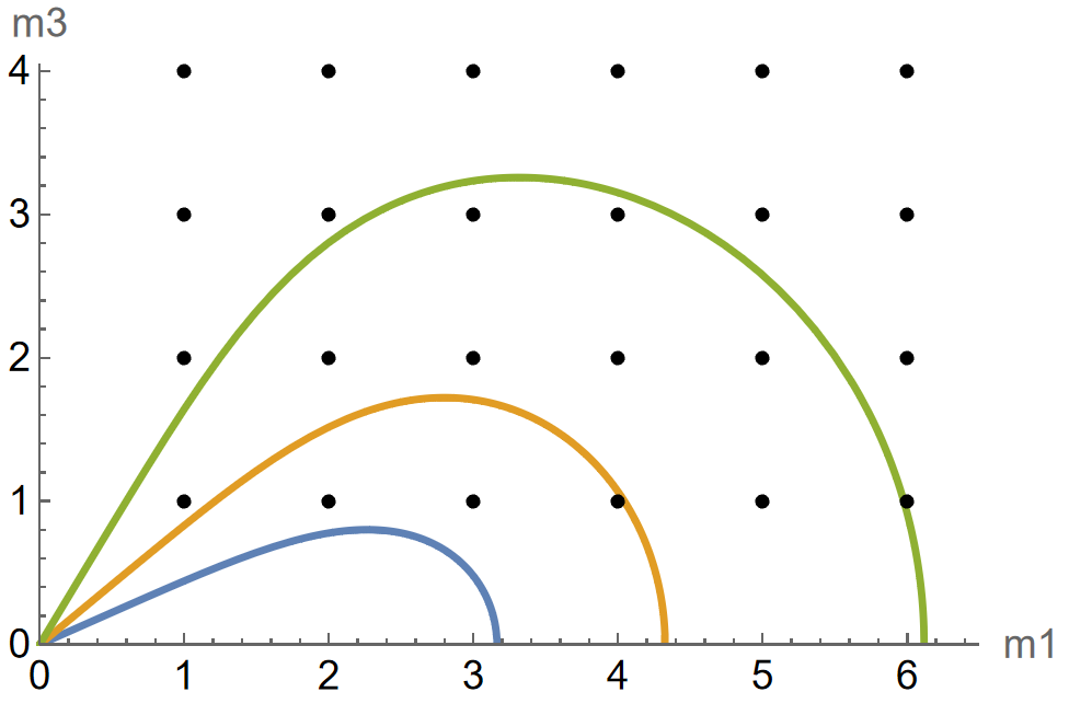
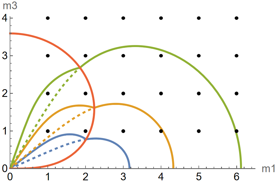
(a)	(b)

Figure 3. (a) Level curves of $\mathcal{R}^{c}_{0,\textbf{m}}$ for $\mathsf{P}=2$, $\mathscr{R}=10\sqrt{5}$, $k_{1}=1$, and $\mathcal{R}=$ 100 (blue), 350 (yellow) and 1400 (green). (b) For $\mathsf{P}=1/2$, $\mathscr{R}=100\sqrt{5}$, $k_{1}=1$, the boundary curve $\mathscr{R}^{2}=\frac{(\mathsf{P}+1)|\textbf{Km}|^{6}}{(1-\mathsf{P})m_{3}^{2}}$ (red), as well as level curves of $\mathcal{R}^{c}_{0,\textbf{m}}$ and $\mathcal{R}^{(1)}_{0,\textbf{m}}$ (dashed) for $\mathcal{R}=$ 100 (blue), 350 (yellow) and 1400 (green).

Let the index sets $\mathscr{I}_{c,\ell}(\mathfrak{P})$, $\ell=1,2,3,4$, be defined as the collection of indices m such that the eigenvalues of $F^{\textbf{m}}$ have a crossing of type $\ell$ at a given Rayleigh number $\mathcal{R}$. For $\mathsf{P}\geq 1$ these are defined explicitly as

$$\mathscr{I}_{c,1}(\mathfrak{P})=\{\textbf{m}\in\mathbb{N}^{2}:\mathcal{R}_{0,\textbf{m}}^{(1)}=\mathcal{R}\}\hskip 28.45274pt\text{ , }\hskip 28.45274pt\mathscr{I}_{c,2}(\mathfrak{P})=\mathscr{I}_{c,3}(\mathfrak{P})=\mathscr{I}_{c,4}(\mathfrak{P})=\varnothing,$$

whereas for $0<\mathsf{P}<1$, these are defined as

$$\begin{split}\mathscr{I}_{c,1}(\mathfrak{P})=\{\textbf{m}\in\mathbb{N}^{2}:\mathcal{R}_{0,\textbf{m}}^{(1)}=\mathcal{R}\text{ , }\mathscr{R}^{2}<\frac{(\mathsf{P}+1)|\textbf{Km}|^{6}}{(1-\mathsf{P})m_{3}^{2}}\}\hskip 2.84544pt&\text{ , }\hskip 2.84544pt\mathscr{I}_{c,2}(\mathfrak{P})=\{\textbf{m}\in\mathbb{N}^{2}:\mathcal{R}_{0,\textbf{m}}^{(2)}=\mathcal{R}\text{ , }\mathscr{R}^{2}>\frac{(\mathsf{P}+1)|\textbf{Km}|^{6}}{(1-\mathsf{P})m_{3}^{2}}\},\\ \mathscr{I}_{c,3}(\mathfrak{P})=\{\textbf{m}\in\mathbb{N}^{2}:\mathcal{R}_{0,\textbf{m}}^{(1)}=\mathcal{R}\text{ , }\mathscr{R}^{2}>\frac{(\mathsf{P}+1)|\textbf{Km}|^{6}}{(1-\mathsf{P})m_{3}^{2}}\}\hskip 2.84544pt&\text{ , }\hskip 2.84544pt\mathscr{I}_{c,4}(\mathfrak{P})=\{\textbf{m}\in\mathbb{N}^{2}:\mathcal{R}_{0,\textbf{m}}^{(1)}=\mathcal{R}\text{ , }\mathscr{R}^{2}=\frac{(\mathsf{P}+1)|\textbf{Km}|^{6}}{(1-\mathsf{P})m_{3}^{2}}\}.\end{split}$$

In the following theorem, it is proven that certain types of local bifurcations occur at the origin as the Rayleigh number is increased through the critical Rayleigh numbers, under certain hypotheses regarding the simultaneous critical modes. Note that this theorem is not meant to be an exhaustive summary of all possible bifurcations, but only a proof of the occurrence of typical bifurcations. For instance, this theorem characterizes the initial instabilities of the origin.

Theorem 3.

For admissible $\mathfrak{P}^{c}=(\mathcal{R}^{c},\mathscr{R},\mathsf{P},k_{1})$, suppose $\cup_{\ell=1}^{4}\mathscr{I}_{c,\ell}(\mathfrak{P}^{c})$ is non-empty. Suppose also for any $\textbf{m},\tilde{\textbf{m}}\in\cup_{\ell=1}^{4}\mathscr{I}_{c,\ell}(\mathfrak{P}^{c})$ with $\textbf{m}\neq\tilde{\textbf{m}}$ one has

(72) $$\big{(}|m_{1}\pm\tilde{m}_{1}|,|m_{3}\pm\tilde{m}_{3}|\big{)}\not\in\cup_{\ell=1}^{4}\mathscr{I}_{c,\ell}(\mathfrak{P}^{c}).$$

Then the PDE (8) undergoes a local bifurcation at $(\textbf{u},\theta,\mathfrak{P})=(0,0,\mathfrak{P}^{c})$ as the Rayleigh number is increased through $\mathcal{R}^{c}$. Under further assumptions regarding simultaneous critical eigenvalues, these bifurcations are classified as follows:

1. If $|\cup_{\ell=1}^{4}\mathscr{I}_{c,\ell}|=1$, then the bifurcation is a supercritical pitchfork bifurcation (if $|\mathscr{I}_{c,1}|=1$ or $|\mathscr{I}_{c,4}|=1$), a supercritical pitchfork bifurcation (if $|\mathscr{I}_{c,2}|=1$) or a subcritical pitchfork bifurcation (if $|\mathscr{I}_{c,3}|=1$).

2. If $|\cup_{\ell=1}^{4}\mathscr{I}_{c,\ell}|>1$ and m is a critical index such that $m_{3}\neq\hat{m}_{3}$ for all $\hat{\textbf{m}}\in\cup_{\ell=1}^{4}\mathscr{I}_{c,\ell}$ distinct from m, then the bifurcation in these critical variables is as described in (i) above.

3. If $|\cup_{\ell=1}^{4}\mathscr{I}_{c,\ell}|=|\mathscr{I}_{c,1}|=2$, $\textbf{m},\hat{\textbf{m}}$ are the critical indices, $m_{3}=\hat{m}_{3}$, and the condition

   (73) $$\frac{\lambda_{\textbf{m},1}|\textbf{Km}|^{2}(\lambda_{\textbf{m},1}-\lambda_{\textbf{m},2})(\lambda_{\textbf{m},1}-\lambda_{\textbf{m},3})}{m_{1}(\mathsf{P}|\textbf{Km}|^{2}+\lambda_{\textbf{m},1})}\neq\frac{\lambda_{\hat{\textbf{m}},1}|\textbf{K}\hat{\textbf{m}}|^{2}(\lambda_{\hat{\textbf{m}},1}-\lambda_{\hat{\textbf{m}},2})(\lambda_{\hat{\textbf{m}},1}-\lambda_{\hat{\textbf{m}},3})}{\hat{m}_{1}(\mathsf{P}|\textbf{K}\hat{\textbf{m}}|^{2}+\lambda_{\hat{\textbf{m}},1})}$$

   is satisfied, then the bifurcation is a simultaneous occurrence of two supercritical pitchfork bifurcations.

Remark 4.4.

While the Hopf-bifurcations occuring due to crossings of type 2 increase the dimension of the unstable manifold of the origin by two, the subsequent pitchfork bifurcation due to the crossing of type 3 reduces the dimension by one. It therefore follows that at a given Rayleigh number the dimension of the unstable manifold is equal to the number of integer vertices beneath the critical curves in (70). This is proportional to the area under these curves, and since the unstable manifold is a subset of the attractor, one arrives at the following lower bound:

Corollary 4.5.

Let $\mathcal{A}$ be the global attractor of $S(t)$ defined in (55). One has the following bound:

(74) $$d_{Haus}(\mathcal{A})\geq\big{\lfloor}\frac{\sqrt{2}\mathcal{R}^{1/2}}{\sqrt{27}k_{1}(1+\frac{\mathscr{R}^{2}}{\mathcal{R}})}\big{\rfloor}.$$

Remark 4.6.

The set of admissible parameter values for which equality holds in (73) might be empty, although it is quite difficult to prove. However, (73) is easily checked for any fixed set of parameters and fixed pair of indices.

Proof of Theorem 3.

The result follows by first by proving the existence of a parameter dependent invariant manifold in a neighborhood of the origin, determining its lowest orders, then analyzing the reduced system. For the existence proof, one can invoke a parameter dependent center manifold theorem for Hilbert spaces. For definiteness, Theorem 3.3 of Chapter 2 in [14] is invoked here, which states that under certain hypotheses there exists a manifold which is the graph of a smooth function $\Psi$, which contains the origin and is tangent to the center subspace there, and which is locally invariant under the flow defined by (55). The hypotheses are given as follows:

1. Decompose the spectrum of L as $\sigma(\textbf{L})=\sigma_{+}\cup\sigma_{0}\cup\sigma_{-}$, where

   $$\sigma_{\pm}=\{\lambda\in\sigma(\textbf{L}):\pm\mathsf{Re}(\lambda)>0\}\hskip 14.22636pt\text{ , }\hskip 14.22636pt\sigma_{0}=\{\lambda\in\sigma(\textbf{L}):\mathsf{Re}(\lambda)=0\}.$$

   Then $\sigma_{0}$ consists of a finite set of eigenvalues with finite algebraic multiplicity, and L admits a spectral gap, namely there exists a $\gamma>0$ such that

   $$\sup_{\lambda\in\sigma_{-}}\mathsf{Re}(\lambda)<-\gamma\hskip 14.22636pt\text{ , }\hskip 14.22636pt\inf_{\lambda\in\sigma_{+}}\mathsf{Re}(\lambda)>\gamma.$$

2. When working over a Hilbert space $H$, there must exist positive constants $\omega_{0},c>0$, $\alpha\in[0,1)$ such that $i\omega$ belongs to the resolvent set of L for all $\omega\in\mathbb{R}$ with $|\omega|>\omega_{0}$, and

   $$\|(i\omega\mathbb{I}-\textbf{L})^{-1}\|_{C^{0}(H)}\leq\frac{c}{|\omega|}.$$

It’s clear from that the spectrum of L consists only of eigenvalues with finite multiplicity and no continuous spectrum, and Lemma 4.3 together with the discussion above imply that $\mathscr{I}_{c,\ell}$ contain at most finitely many indices, and hence $\sigma_{0}$, $\sigma_{+}$ must be finite as well. Furthermore, Lemma 4.3 also makes it clear that for $\delta>0$ sufficiently small one has a spectral gap for $\mathcal{R}\in[\mathcal{R}^{c}-\delta,\mathcal{R}^{c}+\delta]$. Finally, note that the eigenvalues of $\textbf{L}-i\omega\textbf{I}$ are simply $\lambda-i\omega$, where $\lambda\in\sigma(\textbf{L})$. Since the spectrum has already been determined it is straightforward to check that for $\omega_{0}>0$ sufficiently large one has a bound $|(\lambda-i\omega)^{-1}|\leq c|\omega|^{-1}$ for all $|\omega|>\omega_{0}$ uniform in $\lambda\in\sigma(\textbf{L})$, and the bound for L follows. Hence a center manifold exists.

In order to classify the type of bifurcation that occurs, the Taylor coefficients for $\Psi$ must be determined. As described above, there are finitely many indices m such that the variables $(u^{+}_{\textbf{m}},u^{-}_{\textbf{m}},\theta_{\textbf{m}})$ are critical, and the remaining variables are given by a graph $\Psi$ over these critical variables, which is at least quadratic in the critical variables. In fact, due to the assumption (72) all variables in b, c, as well as any non-critical variables in f must be at least cubic order in the critical variables, hence these do not play a role in determining the type of bifurcation. Thus it suffices to consider the variables in a, f. For $\textbf{m}\in\cup_{\ell=1}^{4}\mathscr{I}_{c,\ell}$, recall from (16) that the critical modes must solve

$$\frac{d}{dt}\begin{pmatrix}u^{+}_{\textbf{m}}\\ u^{-}_{\textbf{m}}\\ \theta_{\textbf{m}}\end{pmatrix}=F^{\textbf{m}}\begin{pmatrix}u^{+}_{\textbf{m}}\\ u^{-}_{\textbf{m}}\\ \theta_{\textbf{m}}\end{pmatrix}-\begin{pmatrix}0\\ 0\\ \mathcal{I}_{\textbf{m}}u_{\textbf{m}}^{+}\theta_{(0,2m_{3})}\end{pmatrix}-\begin{pmatrix}\tilde{N}^{+}_{\textbf{m}}(\textbf{u}^{+},\textbf{u}^{+})\\ \tilde{N}^{-}_{\textbf{m}}(\textbf{u}^{+},\textbf{u}^{-})\\ \tilde{N}^{\theta}_{\textbf{m}}(\textbf{u}^{+},\theta)\end{pmatrix}\hskip 14.22636pt\text{ , }\hskip 14.22636pt\mathcal{I}_{\textbf{m}}=\frac{(-1)^{|\textbf{m}|_{1}}k_{1}}{\sqrt{2}|\textbf{Km}|V},$$

whereas, due to the invariance condition, the stratified temperature mode $\theta_{(0,2m_{3})}$ must solve

$$0=-4m_{3}^{2}\theta_{(0,2m_{3})}+\sum_{\begin{subarray}{c}\tilde{\textbf{m}}\in\cup_{\ell=1}^{4}\mathscr{I}_{c,\ell}\\ \tilde{m}_{3}=m_{3}\end{subarray}}\mathcal{I}_{\tilde{\textbf{m}}}u_{\tilde{\textbf{m}}}^{+}\theta_{\tilde{\textbf{m}}}-\tilde{N}^{\theta}_{(0,2m_{3})}(\textbf{u}^{+},\theta),$$

where due to (72) the nonlinear terms $\tilde{N}$ consist of quadratic terms in which at most one term is critical. These therefore contribute only terms which are quartic in the critical variables and can be neglected. The next step is to diagonalize $F^{\textbf{m}}$ for each critical mode by changing variables with its matrix of eigenvectors $V^{\textbf{m}}$. Note that evaluating the characteristic equation at $\lambda_{\textbf{m}}=-|\textbf{Km}|^{2}$ and $-\mathsf{P}|\textbf{Km}|^{2}$ gives $k_{1}^{2}m_{1}^{2}\mathsf{P}\mathcal{R}(1-\mathsf{P})$ and $m_{3}^{2}\mathsf{P}^{2}\mathscr{R}^{2}(1-\mathsf{P})$ respectively, hence these are not eigenvalues if $\mathsf{P}\neq 1$ and $\mathcal{R},\mathscr{R}>0$. Hence the following matrix of eigenvectors is well defined:

(75) $$V^{\textbf{m}}=\begin{pmatrix}|\textbf{Km}|&|\textbf{Km}|&|\textbf{Km}|\\ \frac{-\mathsf{P}\mathscr{R}m_{3}}{(\mathsf{P}|\textbf{Km}|^{2}+\lambda_{\textbf{m},1})}&\frac{-\mathsf{P}\mathscr{R}m_{3}}{(\mathsf{P}|\textbf{Km}|^{2}+\lambda_{\textbf{m},2})}&\frac{-\mathsf{P}\mathscr{R}m_{3}}{(\mathsf{P}|\textbf{Km}|^{2}+\lambda_{\textbf{m},3})}\\ \frac{(-1)^{|\textbf{m}|_{1}+1}k_{1}m_{1}}{(|\textbf{Km}|^{2}+\lambda_{\textbf{m},1})}&\frac{(-1)^{|\textbf{m}|_{1}+1}k_{1}m_{1}}{(|\textbf{Km}|^{2}+\lambda_{\textbf{m},2})}&\frac{(-1)^{|\textbf{m}|_{1}+1}k_{1}m_{1}}{(|\textbf{Km}|^{2}+\lambda_{\textbf{m},3})}\end{pmatrix}.$$

Denoting $\check{V}^{\textbf{m}}=(V^{\textbf{m}})^{-1}$, one finds

$$\check{V}^{\textbf{m}}=\begin{pmatrix}-\frac{(\mathsf{P}|\textbf{Km}|^{2}+\lambda_{\textbf{m},1})(|\textbf{Km}|^{2}+\lambda_{\textbf{m},1})}{|\textbf{Km}|\big{(}\lambda_{\textbf{m},1}-\lambda_{\textbf{m},2}\big{)}\big{(}\lambda_{\textbf{m},3}-\lambda_{\textbf{m},1}\big{)}}&\frac{-\mathsf{P}\mathscr{R}m_{3}(|\textbf{Km}|^{2}+\lambda_{\textbf{m},1})}{|\textbf{Km}|^{2}\big{(}\lambda_{\textbf{m},1}-\lambda_{\textbf{m},2}\big{)}\big{(}\lambda_{\textbf{m},3}-\lambda_{\textbf{m},1}\big{)}}&\frac{(-1)^{|\textbf{m}|_{1}}\mathsf{P}\mathcal{R}k_{1}m_{1}(\mathsf{P}|\textbf{Km}|^{2}+\lambda_{\textbf{m},1})}{|\textbf{Km}|^{2}\big{(}\lambda_{\textbf{m},1}-\lambda_{\textbf{m},2}\big{)}\big{(}\lambda_{\textbf{m},3}-\lambda_{\textbf{m},1}\big{)}}\\ -\frac{(\mathsf{P}|\textbf{Km}|^{2}+\lambda_{\textbf{m},2})(|\textbf{Km}|^{2}+\lambda_{\textbf{m},2})}{|\textbf{Km}|\big{(}\lambda_{\textbf{m},1}-\lambda_{\textbf{m},2}\big{)}\big{(}\lambda_{\textbf{m},2}-\lambda_{\textbf{m},3}\big{)}}&\frac{-\mathsf{P}\mathscr{R}m_{3}(|\textbf{Km}|^{2}+\lambda_{\textbf{m},2})}{|\textbf{Km}|^{2}\big{(}\lambda_{\textbf{m},1}-\lambda_{\textbf{m},2}\big{)}\big{(}\lambda_{\textbf{m},2}-\lambda_{\textbf{m},3}\big{)}}&\frac{(-1)^{|\textbf{m}|_{1}}\mathsf{P}\mathcal{R}k_{1}m_{1}(\mathsf{P}|\textbf{Km}|^{2}+\lambda_{\textbf{m},2})}{|\textbf{Km}|^{2}\big{(}\lambda_{\textbf{m},1}-\lambda_{\textbf{m},2}\big{)}\big{(}\lambda_{\textbf{m},2}-\lambda_{\textbf{m},3}\big{)}}\\ -\frac{(\mathsf{P}|\textbf{Km}|^{2}+\lambda_{\textbf{m},3})(|\textbf{Km}|^{2}+\lambda_{\textbf{m},3})}{|\textbf{Km}|\big{(}\lambda_{\textbf{m},2}-\lambda_{\textbf{m},3}\big{)}\big{(}\lambda_{\textbf{m},3}-\lambda_{\textbf{m},1}\big{)}}&\frac{-\mathsf{P}\mathscr{R}m_{3}(|\textbf{Km}|^{2}+\lambda_{\textbf{m},3})}{|\textbf{Km}|^{2}\big{(}\lambda_{\textbf{m},2}-\lambda_{\textbf{m},3}\big{)}\big{(}\lambda_{\textbf{m},3}-\lambda_{\textbf{m},1}\big{)}}&\frac{(-1)^{|\textbf{m}|_{1}}\mathsf{P}\mathcal{R}k_{1}m_{1}(\mathsf{P}|\textbf{Km}|^{2}+\lambda_{\textbf{m},3})}{|\textbf{Km}|^{2}\big{(}\lambda_{\textbf{m},2}-\lambda_{\textbf{m},3}\big{)}\big{(}\lambda_{\textbf{m},3}-\lambda_{\textbf{m},1}\big{)}}\end{pmatrix}.$$

On the other hand, for $\mathsf{P}=1$ one has $\lambda_{\textbf{m},2}=-|\textbf{Km}|^{2}$, hence the above formula is not well-defined, but here one can use the explicit expressions from (68). In this case $V^{\textbf{m}}$, $\check{V}^{\textbf{m}}$ are given by

$$\begin{pmatrix}|\textbf{Km}|&0&|\textbf{Km}|\\ \frac{-\mathscr{R}m_{3}|\textbf{Km}|}{\sqrt{k_{1}^{2}m_{1}^{2}\mathcal{R}-m_{3}^{2}\mathscr{R}^{2}}}&(-1)^{|\textbf{m}|_{1}}\mathcal{R}k_{1}m_{1}&\frac{\mathscr{R}m_{3}|\textbf{Km}|}{\sqrt{k_{1}^{2}m_{1}^{2}\mathcal{R}-m_{3}^{2}\mathscr{R}^{2}}}\\ \frac{(-1)^{|\textbf{m}|_{1}+1}k_{1}m_{1}|\textbf{Km}|}{\sqrt{k_{1}^{2}m_{1}^{2}\mathcal{R}-m_{3}^{2}\mathscr{R}^{2}}}&\mathscr{R}m_{3}&\frac{(-1)^{|\textbf{m}|_{1}}k_{1}m_{1}|\textbf{Km}|}{\sqrt{k_{1}^{2}m_{1}^{2}\mathcal{R}-m_{3}^{2}\mathscr{R}^{2}}}\end{pmatrix}\text{ , }\begin{pmatrix}\frac{1}{2|\textbf{Km}|}&\frac{m_{3}\mathscr{R}}{2|\textbf{Km}|\sqrt{k_{1}^{2}m_{1}^{2}\mathcal{R}-m_{3}^{2}\mathscr{R}^{2}}}&\frac{(-1)^{|\textbf{m}|_{1}+1}k_{1}m_{1}\mathcal{R}}{2|\textbf{Km}|\sqrt{k_{1}^{2}m_{1}^{2}\mathcal{R}-m_{3}^{2}\mathscr{R}^{2}}}\\ 0&\frac{(-1)^{|\textbf{m}|_{1}}k_{1}m_{1}}{k_{1}^{2}m_{1}^{2}\mathcal{R}-m_{3}^{2}\mathscr{R}^{2}}&\frac{-m_{3}\mathscr{R}}{k_{1}^{2}m_{1}^{2}\mathcal{R}-m_{3}^{2}\mathscr{R}^{2}}\\ \frac{1}{2|\textbf{Km}|}&\frac{-m_{3}\mathscr{R}}{2|\textbf{Km}|\sqrt{k_{1}^{2}m_{1}^{2}\mathcal{R}-m_{3}^{2}\mathscr{R}^{2}}}&\frac{(-1)^{|\textbf{m}|_{1}}k_{1}m_{1}\mathcal{R}}{2|\textbf{Km}|\sqrt{k_{1}^{2}m_{1}^{2}\mathcal{R}-m_{3}^{2}\mathscr{R}^{2}}}\end{pmatrix},$$

respectively. Defining the change of variables

$$\begin{pmatrix}w_{1}^{\textbf{m}}\\ w_{2}^{\textbf{m}}\\ w_{3}^{\textbf{m}}\end{pmatrix}=\check{V}^{\textbf{m}}\begin{pmatrix}u^{+}_{\textbf{m}}\\ u^{-}_{\textbf{m}}\\ \theta_{\textbf{m}}\end{pmatrix},$$

one finds the stratified temperature mode is given up to cubic order by

(76) $$\theta_{(0,2m_{3})}=\frac{1}{4m_{3}^{2}}\sum_{\begin{subarray}{c}\tilde{\textbf{m}}\in\cup_{\ell=1}^{4}\mathscr{I}_{c,\ell}\\ \tilde{m}_{3}=m_{3}\end{subarray}}\mathcal{I}_{\tilde{\textbf{m}}}\sum_{\tilde{j}\leq 3}v_{1,\tilde{j}}^{\tilde{\textbf{m}}}w_{\tilde{j}}^{\tilde{\textbf{m}}}\sum_{\hat{j}\leq 3}v_{3,\hat{j}}^{\tilde{\textbf{m}}}w_{\hat{j}}^{\tilde{\textbf{m}}},$$

and hence up to cubic order the $w_{j}^{\textbf{m}}$ must solve

(77) $$\frac{d}{dt}\begin{pmatrix}w_{1}^{\textbf{m}}\\ w_{2}^{\textbf{m}}\\ w_{3}^{\textbf{m}}\end{pmatrix}=\begin{pmatrix}\lambda_{\textbf{m},1}w_{1}^{\textbf{m}}\\ \lambda_{\textbf{m},2}w_{2}^{\textbf{m}}\\ \lambda_{\textbf{m},3}w_{3}^{\textbf{m}}\end{pmatrix}-\frac{\mathcal{I}_{\textbf{m}}}{4m_{3}^{2}}\begin{pmatrix}\check{v}_{1,3}^{\textbf{m}}\\ \check{v}_{2,3}^{\textbf{m}}\\ \check{v}_{3,3}^{\textbf{m}}\end{pmatrix}\sum_{j\leq 3}v_{1,j}^{\textbf{m}}w_{j}^{\textbf{m}}\sum_{\begin{subarray}{c}\tilde{\textbf{m}}\in\cup_{\ell=1}^{4}\mathscr{I}_{c,\ell}\\ \tilde{m}_{3}=m_{3}\end{subarray}}\mathcal{I}_{\tilde{\textbf{m}}}\sum_{\tilde{j}\leq 3}v_{1,\tilde{j}}^{\tilde{\textbf{m}}}w_{\tilde{j}}^{\tilde{\textbf{m}}}\sum_{\hat{j}\leq 3}v_{3,\hat{j}}^{\tilde{\textbf{m}}}w_{\hat{j}}^{\tilde{\textbf{m}}}.$$

From this point, the cases above must be considered individually. First, consider the case $|\cup_{\ell=1}^{4}\mathscr{I}_{c,\ell}|=1$. Note in this case the sum over $\tilde{\textbf{m}}$ consists only of the single term $\tilde{\textbf{m}}=\textbf{m}$. If $|\mathscr{I}_{c,1}|=1$, then since $w_{2}^{\textbf{m}}$, $w_{3}^{\textbf{m}}$ are non-critical, they are at least quadratic in $w_{1}^{\textbf{m}}$. First considering the case $\mathsf{P}\neq 1$, the equation for $w_{1}^{\textbf{m}}$ becomes as follows, up to cubic order:

(78) $$\frac{d}{dt}w_{1}^{\textbf{m}}=\lambda_{\textbf{m},1}w_{1}^{\textbf{m}}-\frac{\mathcal{I}_{\textbf{m}}^{2}}{4m_{3}^{2}}\frac{\mathsf{P}\mathcal{R}k_{1}^{2}m_{1}^{2}(\mathsf{P}|\textbf{Km}|^{2}+\lambda_{\textbf{m},1})}{(|\textbf{Km}|^{2}+\lambda_{\textbf{m},1})(\lambda_{\textbf{m},1}-\lambda_{\textbf{m},2})(\lambda_{\textbf{m},1}-\lambda_{\textbf{m},3})}\big{(}w_{1}^{\textbf{m}}\big{)}^{3}.$$

Since $\lambda_{\textbf{m},2},\lambda_{\textbf{m},3}$ have negative real part bounded away from zero, and are either real or conjugate pairs, the coefficient of the cubic term is strictly negative, and hence the system undergoes a supercritical pitchfork bifurcation at $\mathcal{R}^{c}$. On the other hand, for $\mathsf{P}=1$, the equation for $w_{1}^{\textbf{m}}$ becomes as follows, yielding the same result:

$$\frac{d}{dt}w_{1}^{\textbf{m}}=\lambda_{\textbf{m},1}w_{1}^{\textbf{m}}-\frac{\mathcal{I}_{\textbf{m}}^{2}|\textbf{Km}|^{2}\mathcal{R}k_{1}^{2}m_{1}^{2}}{8m_{3}^{2}(k_{1}^{2}m_{1}^{2}\mathcal{R}-m_{3}^{2}\mathscr{R}^{2})}\big{(}w_{1}^{\textbf{m}}\big{)}^{3}.$$

If instead $|\mathscr{I}_{c,2}|=1$, then due to the fact that $(u_{\textbf{m}}^{+},u_{\textbf{m}}^{-},\theta_{\textbf{m}})$ are real, $w_{1}^{\textbf{m}},w_{2}^{\textbf{m}}$ must be complex conjugates, hence let $\rho\geq 0$ and $\phi>0$ be such that $w_{1}^{\textbf{m}}=\rho e^{i\phi},w_{2}^{\textbf{m}}=\rho e^{-i\phi}$. Up to cubic order the equations for $w_{1}^{\textbf{m}},w_{2}^{\textbf{m}}$ are

$$\begin{split}\frac{d}{dt}w_{1}^{\textbf{m}}&=\lambda_{\textbf{m},1}w_{1}^{\textbf{m}}-\frac{\mathcal{I}_{\textbf{m}}^{2}}{4m_{3}^{2}}\frac{\mathsf{P}\mathcal{R}k_{1}^{2}m_{1}^{2}(\mathsf{P}|\textbf{Km}|^{2}+\lambda_{\textbf{m},1})}{(\lambda_{\textbf{m},1}-\lambda_{\textbf{m},2})(\lambda_{\textbf{m},1}-\lambda_{\textbf{m},3})}\big{(}w_{1}^{\textbf{m}}+w_{2}^{\textbf{m}}\big{)}^{2}\big{(}\frac{w_{1}^{\textbf{m}}}{|\textbf{Km}|^{2}+\lambda_{\textbf{m},1}}+\frac{w_{2}^{\textbf{m}}}{|\textbf{Km}|^{2}+\lambda_{\textbf{m},2}}\big{)}\\ \frac{d}{dt}w_{2}^{\textbf{m}}&=\lambda_{\textbf{m},2}w_{2}^{\textbf{m}}+\frac{\mathcal{I}_{\textbf{m}}^{2}}{4m_{3}^{2}}\frac{\mathsf{P}\mathcal{R}k_{1}^{2}m_{1}^{2}(\mathsf{P}|\textbf{Km}|^{2}+\lambda_{\textbf{m},2})}{(\lambda_{\textbf{m},1}-\lambda_{\textbf{m},2})(\lambda_{\textbf{m},2}-\lambda_{\textbf{m},3})}\big{(}w_{1}^{\textbf{m}}+w_{2}^{\textbf{m}}\big{)}^{2}\big{(}\frac{w_{1}^{\textbf{m}}}{|\textbf{Km}|^{2}+\lambda_{\textbf{m},1}}+\frac{w_{2}^{\textbf{m}}}{|\textbf{Km}|^{2}+\lambda_{\textbf{m},2}}\big{)}.\end{split}$$

Using the chain rule and Taylor expanding the resulting sinusoids, it follows that $\rho$ and $\phi$ must solve

(79) $$\begin{split}\frac{d}{dt}\rho&=\mathsf{Re}(\lambda_{\textbf{m},1})\rho+\frac{\mathcal{I}_{\textbf{m}}^{2}k_{1}^{2}m_{1}^{2}\mathsf{P}\mathcal{R}\big{(}\mathsf{P}|\textbf{Km}|^{2}+\mathsf{Re}(\lambda_{\textbf{m},1})\big{)}\big{(}\mathsf{P}|\textbf{Km}|^{2}+\lambda_{\textbf{m},3}\big{)}}{m_{3}^{2}||\textbf{Km}|^{2}+\lambda_{\textbf{m},1}|^{2}|\lambda_{\textbf{m},1}-\lambda_{\textbf{m},3}|^{2}}\rho^{3}+\mathscr{O}(\rho^{3}\phi^{4})\\ \frac{d}{dt}\phi&=\mathsf{Im}(\lambda_{\textbf{m},1})+\mathscr{O}(\rho^{2}),\end{split}$$

and since $\lambda_{\textbf{m},3}<-\mathsf{P}|\textbf{Km}|^{2}$ on a neighborhood of $\mathcal{R}^{c}$, it is clear that coefficient of $\rho^{3}$ is negative, hence the system undergoes a supercritical Hopf bifurcation at $\mathcal{R}^{c}$. If $|\mathscr{I}_{c,3}|=1$, all eigenvalues and variables $w_{j}^{\textbf{m}}$ are real, $\lambda_{\textbf{m},1}>0$ and $w_{2}^{\textbf{m}}$ is the only critical variable. In this case, the equation for $w_{2}^{\textbf{m}}$ is as follows, up to cubic order:

$$\frac{d}{dt}w_{2}^{\textbf{m}}=\lambda_{\textbf{m},2}w_{2}^{\textbf{m}}+\frac{\mathcal{I}_{\textbf{m}}^{2}}{4m_{3}^{2}}\frac{\mathsf{P}\mathcal{R}k_{1}^{2}m_{1}^{2}(\mathsf{P}|\textbf{Km}|^{2}+\lambda_{\textbf{m},2})}{(|\textbf{Km}|^{2}+\lambda_{\textbf{m},2})(\lambda_{\textbf{m},1}-\lambda_{\textbf{m},2})(\lambda_{\textbf{m},2}-\lambda_{\textbf{m},3})}\big{(}w_{2}^{\textbf{m}}\big{)}^{3}.$$

Since the coefficient of the cubic term is strictly positive, and since $\lambda_{\textbf{m},2}$ is decreasing from positive to negative as the Rayleigh number increases through $\mathcal{R}^{c}$, the system undergoes a subcritical pitchfork bifurcation. Finally, if $|\mathscr{I}_{c,4}|=1$ then (79) is valid for $\mathcal{R}<\mathcal{R}^{c}$ and (78) is valid for $\mathcal{R}>\mathcal{R}^{c}$. These imply that on the invariant manifold the origin is the only fixed point for $\mathcal{R}<\mathcal{R}^{c}$, and two non-trivial fixed points emerge for $\mathcal{R}>\mathcal{R}^{c}$ which are locally stable with respect to the flow on the invariant manifold, and hence a supercritical pitchfork bifurcation occurs.

It is clear for $|\cup_{\ell=1}^{4}\mathscr{I}_{c,\ell}|>1$ and a critical index m such that $m_{3}\neq\hat{m}_{3}$ for any distinct $\hat{m}\in\cup_{\ell=1}^{4}\mathscr{I}_{c,\ell}$ that m does not interact with any other critical mode through the stratified temperature mode in (76) to cubic order, and the above analysis carries through for this critical index.

Finally, consider the case $|\cup_{\ell=1}^{4}\mathscr{I}_{c,\ell}|=|\mathscr{I}_{c,1}|=2$ with $m_{3}=\hat{m}_{3}$. In this case the solution for the stratified temperature in (76) contains both critical modes $w_{1}^{\textbf{m}}$, $w_{1}^{\hat{\textbf{m}}}$. Considering first the case $\mathsf{P}\neq 1$, the equations for these modes become as follows up to cubic order:

$$\begin{split}\frac{dw_{1}^{\textbf{m}}}{dt}&=\lambda_{\textbf{m},1}w_{1}^{\textbf{m}}-\frac{c_{1}m_{1}(\mathsf{P}|\textbf{Km}|^{2}+\lambda_{\textbf{m},1})w_{1}^{\textbf{m}}}{|\textbf{Km}|^{2}(\lambda_{\textbf{m},1}-\lambda_{\textbf{m},2})(\lambda_{\textbf{m},1}-\lambda_{\textbf{m},3})}\Big{(}\frac{m_{1}\big{(}w_{1}^{\textbf{m}}\big{)}^{2}}{(|\textbf{Km}|^{2}+\lambda_{\textbf{m},1})}+\frac{\hat{m}_{1}\big{(}w_{1}^{\hat{\textbf{m}}}\big{)}^{2}}{(|\textbf{K}\hat{\textbf{m}}|^{2}+\lambda_{\hat{\textbf{m}},1})}\Big{)}+\mathscr{O}\big{(}w_{1}^{\textbf{m}}(w_{1}^{\textbf{m}}+w_{1}^{\hat{\textbf{m}}})^{3}\big{)}\\ \frac{dw_{1}^{\hat{\textbf{m}}}}{dt}&=\lambda_{\hat{\textbf{m}},1}w_{1}^{\hat{\textbf{m}}}-\frac{c_{1}\hat{m}_{1}(\mathsf{P}|\textbf{K}\hat{\textbf{m}}|^{2}+\lambda_{\hat{\textbf{m}},1})w_{1}^{\hat{\textbf{m}}}}{|\textbf{K}\hat{\textbf{m}}|^{2}(\lambda_{\hat{\textbf{m}},1}-\lambda_{\hat{\textbf{m}},2})(\lambda_{\hat{\textbf{m}},1}-\lambda_{\hat{\textbf{m}},3})}\Big{(}\frac{m_{1}\big{(}w_{1}^{\textbf{m}}\big{)}^{2}}{(|\textbf{Km}|^{2}+\lambda_{\textbf{m},1})}+\frac{\hat{m}_{1}\big{(}w_{1}^{\hat{\textbf{m}}}\big{)}^{2}}{(|\textbf{K}\hat{\textbf{m}}|^{2}+\lambda_{\hat{\textbf{m}},1})}\Big{)}+\mathscr{O}\big{(}w_{1}^{\hat{\textbf{m}}}(w_{1}^{\textbf{m}}+w_{1}^{\hat{\textbf{m}}})^{3}\big{)}.\end{split}$$

in which $c_{1}=\frac{\mathsf{P}\mathcal{R}k_{1}^{5}}{4\pi^{2}m_{3}^{2}}$. In this case the coefficient of the cubic terms are negative, hence for $\mathcal{R}\leq\mathcal{R}^{c}$ the origin is the only solution. On the other hand, for $\mathcal{R}>\mathcal{R}^{c}$ one must check the condition (73). If equality does not hold, then the above two equations are not equivalent, and hence distinct non-trivial solutions can be found from each of the above via the implicit function theorem.

∎

5. Numerical analysis

This section summarizes some numerical investigations into heat transport in the Boussinesq Coriolis model via the HKC models. These aim at investigating the following issues:

1. Convergence in time issues: How long must one integrate a trajectory to obtain an approximation of the infinite time average? How large are the errors associated with step-size, especially for solutions which appear chaotic (ie persistent errors)?

2. PDE approximation by the ODE’s: For a given $\mathcal{R},\mathscr{R}$, what is the heat transport exhibited by the Boussinesq Coriolis model, ie how large must $M$ be such that all subsequent models agree? How does this compare to the bounds in section 4? How large is the error associated with using an insufficiently large model?

3. Dynamical issues: What are the dynamically stable values of the heat transport (ie heat transport obtained by all initial conditions in a set of positive measure)? At a given Rayleigh number, are there multiple stable heat transport values? What heat transport do stationary solutions exhibit, and how much does this differ from time dependent solutions? Can chaotic solutions be identified?

Therefore this section is broken down as follows. First, a code inventory and a brief overview of some basic phenomenology are given. Next, results comparing the heat transport values for different HKC models calculated over a broad range of $\mathcal{R}$, $\mathscr{R}$ are given. Lastly, the heat transport for stationary solutions is determined using the numerical continuation software MATCONT, and issues regarding dynamic stability are addressed. Note that all of the computations were done using MATLAB on a standard laptop or desktop, and as mentioned above the codes are available on GitHub.

5.1. Code inventory and basic phenomenology

The codes begin with the script ModelConstructor.mat which takes as input a positive integer $M$, and writes a file called HKCM.mat containing the right hand side of (16). Solutions of the HKC-$M$ model can then be simulated with the function FluidSolver.mat, which takes as input the desired parameters $\mathfrak{P}$ and model number $M$, uses ode45 to call HKCM.mat and saves the trajectory along with the parameters. FluidSolver.mat was written so that it can be given an initial condition (either random or near-uniform) and start at $t=0$, or it can continue an already computed trajectory for a specified time. Several codes are then available to visualize the trajectory, either in phase space, or via the corresponding velocity or temperature fields. Several codes are also available to compute the cumulative average heat transport corresponding to these trajectories using the expression (51). The function HeatTransport_Trajectory.mat takes a single trajectory and computes its heat transport, whereas the script HeatTransport_Iterator.mat is initialized with an array of Rayleigh and rotation numbers, computes trajectories for each parameter value by calling FluidSolver.mat and then computes the corresponding heat transport. Crucially, HeatTransport_Iterator.mat then tests the fluctuations in the heat transport value, and either continues the trajectory if the fluctuations are larger than a specified threshold, or saves the data if the fluctuations are acceptably small. For example, Figure 4 depicts the phase diagram and temperature field of a turbulent flow, and the last panel depicts its cumulative average heat transport apparently converging to an infinite time average after initial fluctuations.

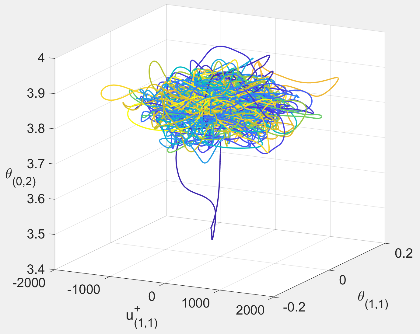
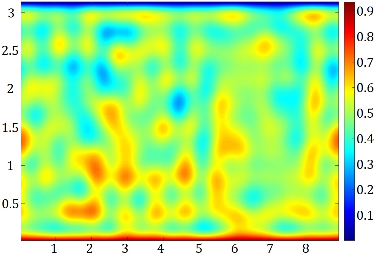
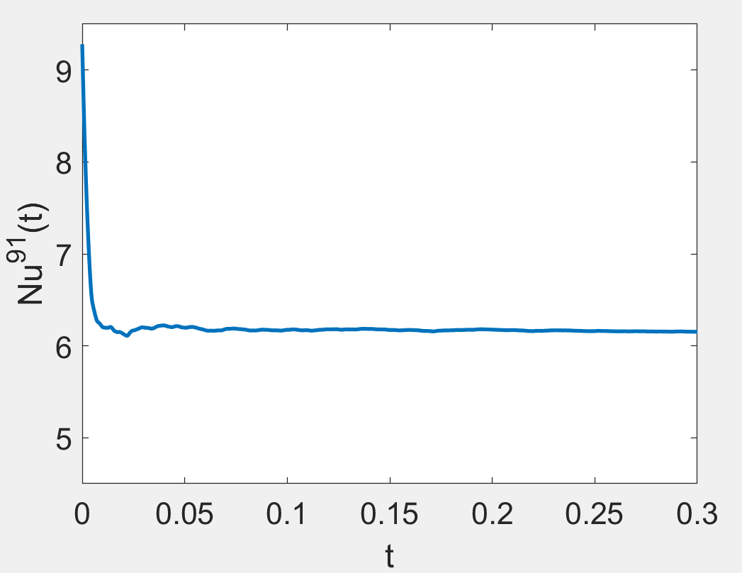
(a)	(b)	(c)

Figure 4. For $(\mathsf{P},k_{1},\mathcal{R},\mathscr{R})=(1,\frac{1}{\sqrt{2}},10^{6},10^{2})$, (a) a trajectory of the HKC-91 model in phase space projected onto the Lorenz triple $(u^{+}_{(1,1)},\theta_{(1,1)},\theta_{(0,2)})$, (b) a snapshot of its temperature field and (c) its cumulative average heat transport.

Figure 5 depicts several phenomena seen throughout all the simulations performed. Both panels in Figure 5 show the heat transport computed for solutions to the HKC-$M$ models as a function $\mathcal{R}$ and $\mathscr{R}$, with initial conditions given by random perturbations from the uniform state $(\textbf{u}_{0},T_{0})=(0,1/2)$. The parameters $(\mathsf{P},k_{1})$ were chosen to equal their classical Lorenz values $(10,1/\sqrt{2})$, since with this choice there is a huge body of literature to compare to. In panel (a), the output for the Lorenz-Stenflo (HKC1) model is depicted, and here it is visible that the heat transport is zero until the first instability $\mathcal{R}_{0,(1,1)}^{c}$, then increases until the attractor becomes chaotic. In the chaotic regime, the heat transport is less than that of the stationary solution, but as one increases the Rayleigh number further, the heat transport levels off to some value. On the other hand, it is also visible that as one increases the rotation number beginning in the chaotic regime, the heat transport first increases as the stationary solution restabilizes, but then decreases to zero as the rotation is increased through the value corresponding to the critical Rayleigh number. In panel (b), it is visible that while the HKC models tend to agree for smaller Rayleigh numbers, for larger Rayleigh numbers the larger HKC models tend to exhibit larger heat transport and more complicated fluctuations, and a slower decay to zero as the rotation number is increased.

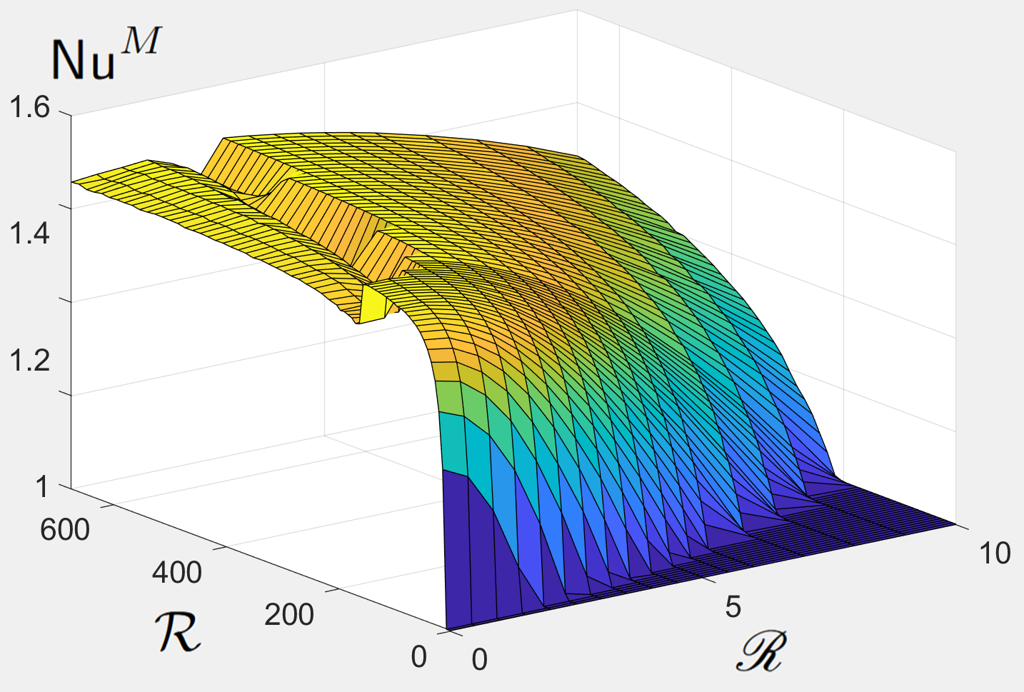
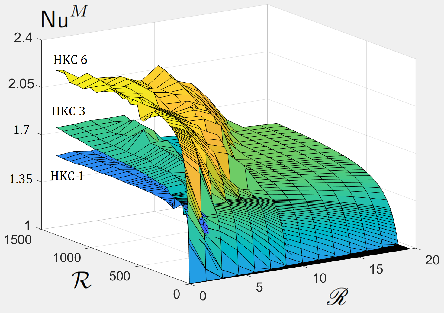
(a)	(b)

Figure 5. For $\mathsf{P}=10$, $k_{1}=\frac{1}{\sqrt{2}}$, plots of the heat transport for the HKC models computed using ode45 with near uniform initial conditions. (a) Plot of the heat transport for the HKC1 model, (b) Plots of the heat transport for the HKC1, HKC3 and HKC6 models.

5.2. Heat transport model comparison

In order to determine the heat transport which might correspond to the full Boussinesq Coriolis model, HeatTransport_Iterator.mat was used generate trajectories of the HKC$M$ models for $M=36$, $45$, $55$, $66$, $78$, $91$ and $105$, corresponding to the $8^{th}$ through $14^{th}$ completed shell. For each model, a trajectory was generated beginning from a random perturbation of the uniform initial condition with $\mathsf{P}=10,$ $k_{1}=1/\sqrt{2}$, and where $\mathcal{R},\mathscr{R}$ range across the following values:

(80) $$\mathcal{R}=[1,(1:1:4)\cdot\frac{10^{2}}{4},(1:1:4)\cdot\frac{10^{3}}{4},(1:1:4)\cdot\frac{10^{4}}{4},(3:1:20)\cdot\frac{10^{5}}{2}]\hskip 14.22636pt\text{ , }\hskip 14.22636pt\mathscr{R}=(0:1:10)\cdot 10^{2}.$$

where $x_{0}:\Delta x:x_{f}$ denotes the set of all integers beginning from $x_{0}$, incrementing by $\Delta x$ and ending with $x_{f}$. For these trajectories, the relative and absolute error in ode45 were set to $10^{-12}$, and in order to account for the faster processes at higher Rayleigh number the time increment was set to $\min(10^{-4},\frac{10}{\mathcal{R}})$. The trajectories were integrated for $10^{4}$ time increments, and the cumulative heat transport was computed. The computations then enter into a loop which extended the trajectory by an additional $10^{3}$ time units until the standard deviation in the second half of the trajectory was less than 2 percent of the cumulative heat transport at the end of the trajectory. The results are shown in Figure 6.

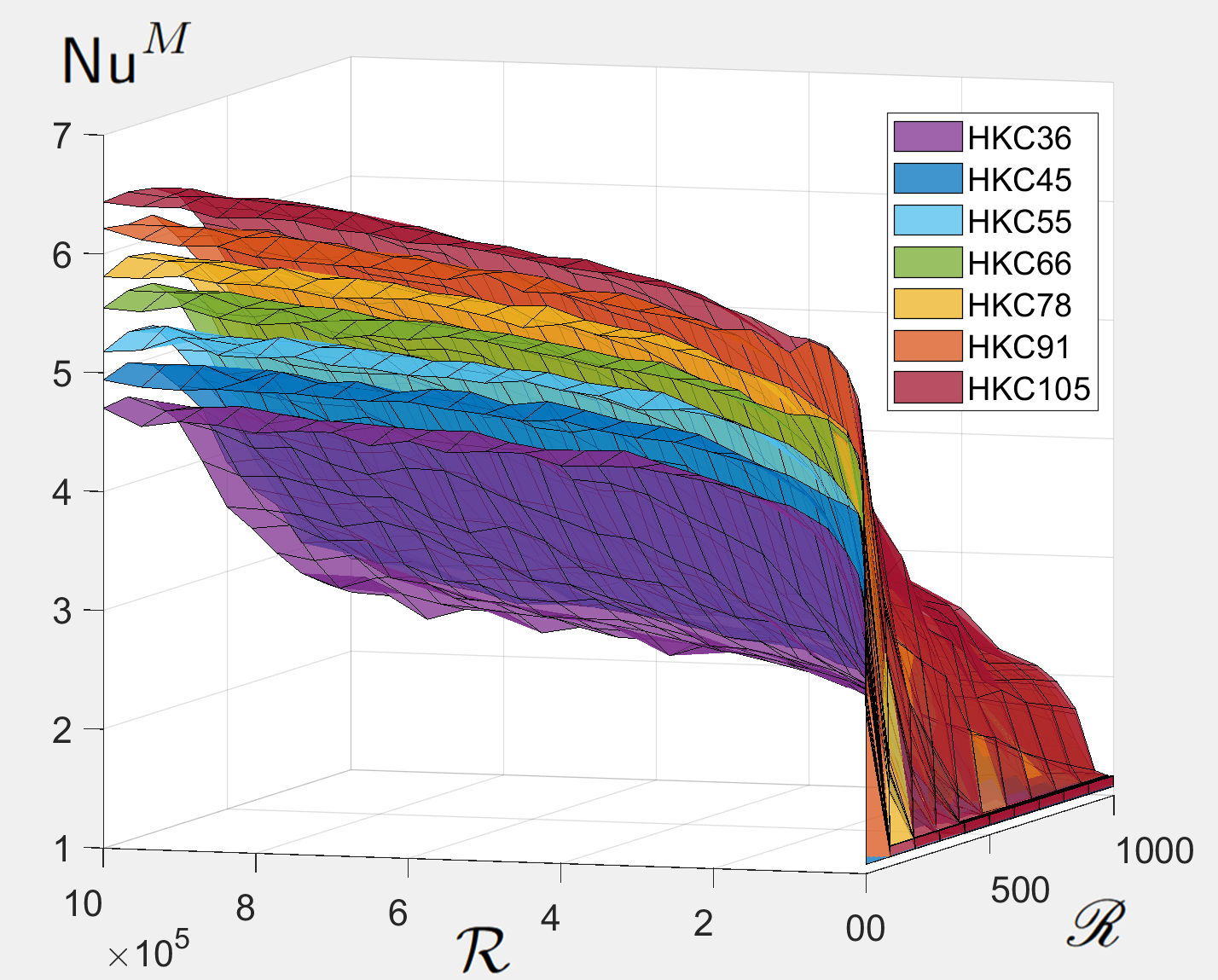
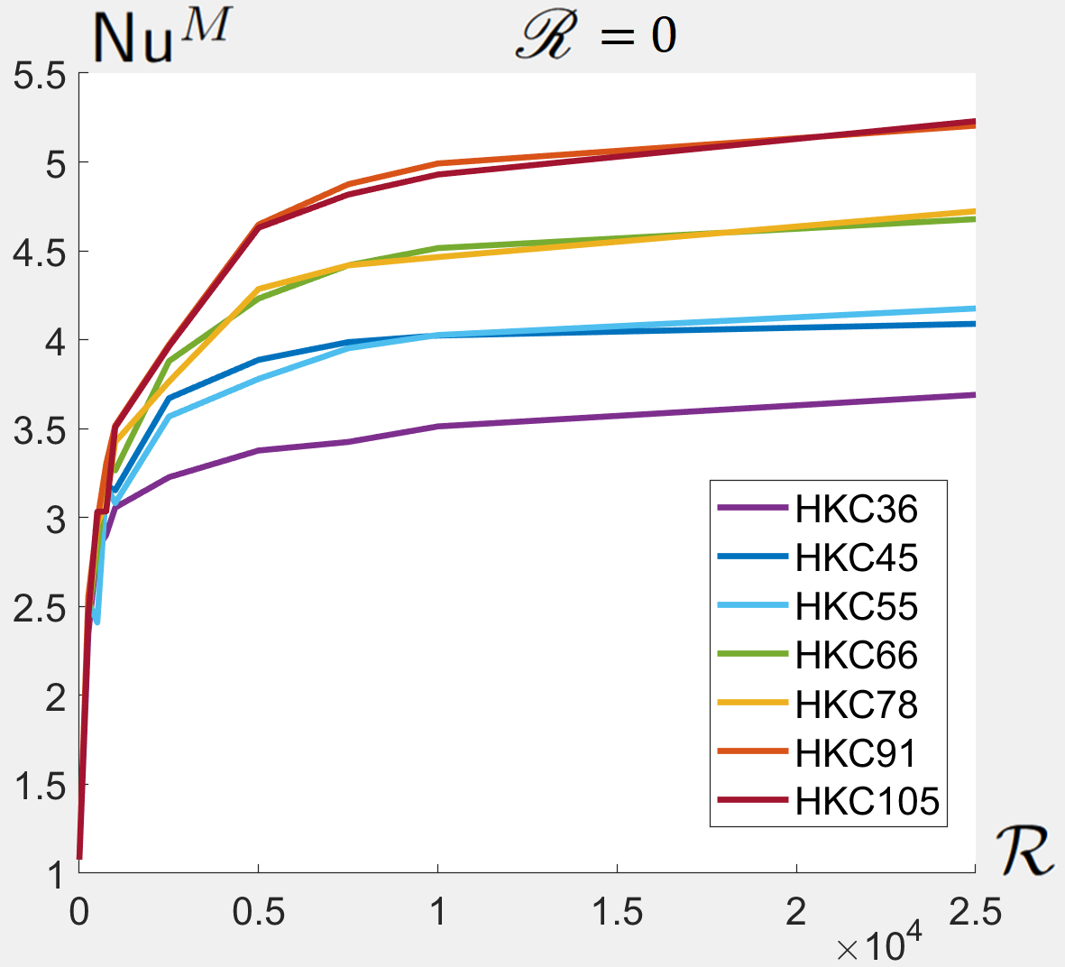
(a)	(b)

Figure 6. Heat transport model comparison (a) for all $\mathcal{R},\mathscr{R}$ in (80) and (b) for $\mathscr{R}=0$, $0\leq\mathcal{R}\leq 2.5\cdot 10^{4}$.

Panel (a) in Figure 6 displays the heat transport for all of the values $\mathcal{R},\mathscr{R}$ in (80). Most prominently, this figure displays that the heat transport for each HKC model increases rather rapidly for low Rayleigh numbers, and the rate of increase slows dramatically for higher Rayleigh numbers, apparently leveling off to a constant value. The width of the region of rapid increase is fairly small, hence panel (b) displays the heat transport for $\mathscr{R}=0$ and for $\mathcal{R}$ only up to $2.5\cdot 10^{4}$, at which point the heat transport of HKC models achieve the same ordering that they possess ever after. The models seem to agree as the heat transport rapidly increases, but one by one they undergo this leveling off phenomena, with lower order models leveling off earlier than higher order models. This suggests a possible mechanism for when the truncated models begins to fail to represent the PDE, namely when the Rayleigh number becomes larger than the viscous force acting on the smallest scale of the truncated model. We’ll return to this point later. As the rotation number increases, Figure 6 shows the heat transport decreasing for all models, although more slowly for larger HKC models. Furthermore the region of agreement increases, and there is an increasingly large interval of Rayleigh numbers for which all models report zero convective transport (ie a Nusselt number of $1$).

In order to provide a more quantitative study of the region of agreement, another set of computations were performed, this time on the smaller, higher resolution set of Rayleigh and rotation numbers given below:

(81) $$\mathcal{R}=[1,(1:1:10)\cdot 50,(6:1:10)\cdot 10^{2},(2:1:5)\cdot 10^{3}]\hskip 14.22636pt\text{ , }\hskip 14.22636pt\mathscr{R}=0:50:300.$$

In this case trajectories were generated for all of the HKC$M$ models with completed shells up to the $14^{th}$ shell, namely for $M=1,$ $3,$ $6,$ $10,$ $15,$ $21,$ $28,$ $36$, $45$, $55$, $66$, $78$, $91$ and $105$. The initial conditions, time increment and other settings were chosen to be the same as before. The heat transport for each Rayleigh and rotation number was then compared across all models, and the lowest dimensional model which was within $10\%$ of the heat transport value from the HKC$105$ model was found. For convenience, the value of the lowest dimension found in this way will be referred to as the empirical Nusselt dimension, $d_{Nusselt}$. In Figure 7 below, panel (a) depicts the heat transport for all models with $\mathscr{R}=0$, in which the heat transport for the HKC105 model is depicted in a thick green line, and the 10% error thresholds are depicted in thick red lines. In panel (b), one can see the plot of $d_{Nusselt}$, indicating the increasing computational cost associated with resolving the flow as the Rayleigh number increases. The lower bound on the Hausdorff dimension found from (74) was found to be quite small compared to the plot of $d_{Nusselt}$. This is not at all surprising, and in fact this is not a meaningful comparison because the attractor must of course be embedded in a larger ambient space. In order to provide a more meaningful comparison, the quantity $d_{unstable}$ was plotted in red in Figure 7 panel (b), defined as the minimal HKC model which contains all of the unstable modes at the origin. The upper bound 62 was not depicted in 7, because this is far larger, on the order of $10^{5}$ for most of the range depicted in Figure 7.

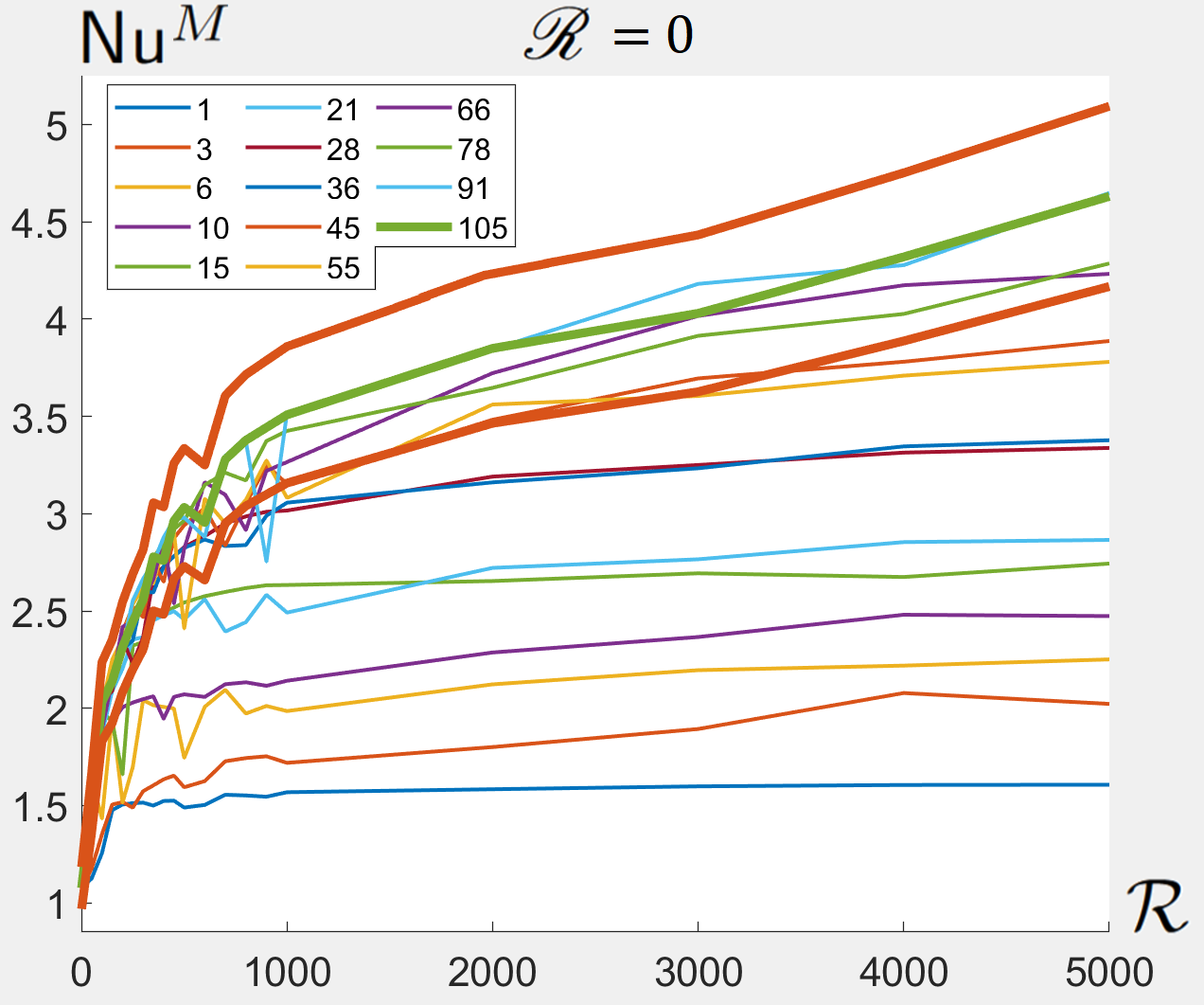
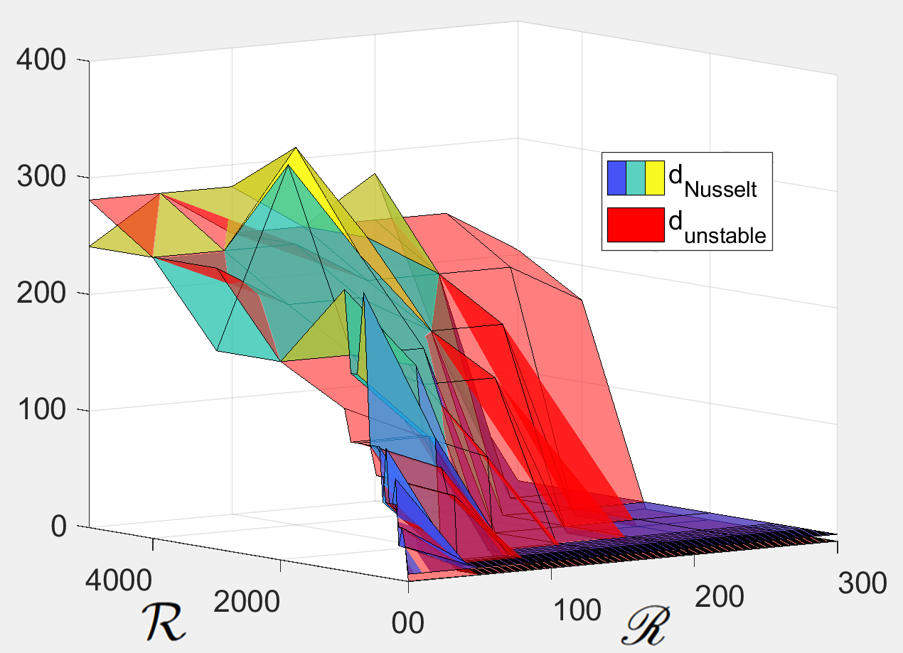
(a)	(b)

Figure 7. (a) Higher resolution heat transport model comparison for $\mathscr{R}=0$, $\mathcal{R}$ as in (81), (b) The computational cost measured by the empirical Nusselt dimension $d_{Nusselt}$ vs. the dimension of the minimal HKC model containing all unstable modes $d_{unstable}$.

The two graphs plotted in panel (b) seem to agree fairly well, although for larger rotation numbers it is noticeable that $d_{unstable}$ jumps up immediately to high dimension when the Rayleigh number crosses a critical threshold, whereas $d_{Nusselt}$ ramps up over a larger range of Rayleigh numbers. This is not surprising because the structures developing after a critical threshold are initially small and don’t immediately produce a large change in transport. It is also noticeable that $d_{Nusselt}$ fluctuates in a non-monotonic way. This is surprising, but as we shall see in the coming section this is possibly an artifact of the presence of multiple stable values of transport. Specifically, the comparison across models may be skewed by the fact that trajectories for each model were initialized using random perturbations of the uniform state.

5.3. Heat transport of stationary solutions and dynamic stability

While stationary solutions are important for understanding the dynamics of any system, they are particularly important in Rayleigh-Bénard convection since it is thought that they might be responsible for the maximal heat transport [29, 20]. Hence this subsection present the results on heat transport and stability properties of all equilibria bifurcating from the origin tracked using MATCONT. MATCONT is a MATLAB software project for the numerical continuation and bifurcation study of continuous and discrete parameterized dynamical systems [6].

After some experimentation, the HKC21 model was selected for analysis using MATCONT, since this model was found to be sufficiently high dimensional to represent the PDE over a decent range of Rayleigh numbers, but also sufficiently low dimensional where a host of numerical continuations could be performed. Beginning from the origin, and with parameters $\mathscr{R},\mathsf{P},k_{1}$ fixed at $(0,10,1/\sqrt{2})$, the Rayleigh was increased from $0$ to $2000$, and the bifurcations at the origin were tracked. The equilibria arising at each branch point were then tracked through $\mathcal{R}=2000$, and then the third generation of equilibria were tracked as well. The heat transport along each branch was then computed, and the result is depicted in Figure 8 below. This figure displays the stability information as well, where the heat transport corresponding to locally stable equilibria is depicting in blue vs the heat transport for unstable equilibria is depicted in red. Furthermore, a time dependent solution was computed for each of the following Rayleigh numbers:

$$\mathcal{R}=0:5:2000$$

where each was initialized as a random perturbation of the uniform state. This is depicted in green. A very complicated bifurcation structure is evident in 8. Most interestingly, there appear branches which emerge from the origin as unstable, but later restabilize for a range of Rayleigh numbers by ejecting further unstable equilibria, leading to the presence of multiple stable values of heat transport at a given Rayleigh number. Furthermore, one sees a rather jagged dependence of the branch of time dependent solutions on the Rayleigh number. But it is also clear for smaller Rayleigh numbers that here the time dependent trajectories randomly select which equilibria to approach due to their random initial condition.

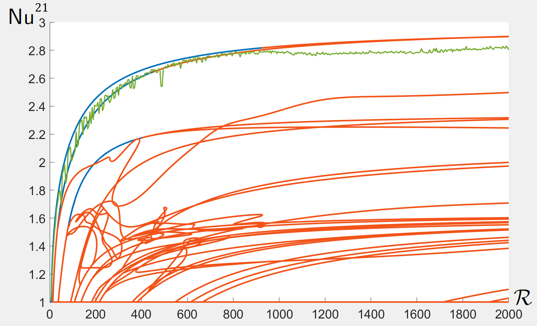
Figure 8. Heat transport bifurcation diagram for HKC21.

One also notices that the branch of time dependent solutions eventually strays from any of the equilibrium branches, but nevertheless exhibits a jagged dependence on the Rayleigh number. Here it is very likely that the time dependent trajectories are randomly switching between multiple stable values of heat transport, but that these stable values are obtained by time dependent solutions. For example, many of the equilibria ultimately lose stability through supercritical Hopf bifurcations. However, the branches corresponding to Hopf bifurcations were found to be very expensive to compute, hence these were not included in Figure 8.

6. Conclusions

This paper has provided several first steps toward a rigorously justified analysis of heat transfer in turbulent geophysical flows. Explicitly computing the formulas for the Galerkin truncations enabled the HKC hierarchy to be implemented in MATLAB in addition to the analytic results on local bifurcations at the origin. Choosing these models to obey balance relations consistent with the PDE also gives consistent dynamical behavior in addition to the energetic consistency desired by climate researchers. The well-posedness theory and upper bound on the attractor dimension carry over from the two-dimensional case, and the rotation in the present case apparently does not ruin the smoothness properties or increase the radius or dimension of the attractor. By studying the local bifurcations at the origin, one mechanism by which the attractor increases in complexity was identified and a rate of increase was given. Furthermore, several heuristic steps toward an analysis of heat transfer were given in the numerical results, from a basic outline of the dependence of the heat transport on the Rayleigh and rotation numbers, to the convergence results as one looks at higher dimensional HKC models, to the results on bifurcations and multi-stability.

Several interesting questions have arisen during the course of writing this paper, which are the goals of future work. First among these is the role of rotation, which seems to play a significant role in numerical simulations and local analytical results but whose effect is absent in the global analytical results. This is due to the fact that many of the global analytical estimates use quadratic expressions such as the kinetic energy $\|\textbf{u}\|_{L^{2}}^{2}$ formed by computing an inner product of a term with itself, and due to the skew-symmetry of the Coriolis term the dependence on rotation disappears. A more general approach is required to resolve the dependence on rotation for Hausdorff dimension bounds or background field arguments. For instance the work of Galdi and Straughan [11] make use of an cleverly chosen Lyapunov function in order to prove that the origin attracts a ball with explicitly determined radius up to the critical Rayleigh number determined by the linear theory. The recent work of Chernyshenko [3] identifies the background field method as equivalent to the auxiliary function method with a quadratic choice of auxiliary function, hence perhaps following this method with a quartic or higher order auxiliary function may resolve the dependence on rotation.

Next is the question of convergence of the Nusselt number with respect to the choice of finite dimensional approximation, the choice of finite integration time and the choice of integration step size. In this paper it was possible to compute heat transport values with a somewhat fine resolution across a wide variety of HKC models since the Rayleigh numbers were chosen only up to $10^{6}$. While higher Rayleigh numbers (perhaps $10^{7}-10^{8}$) and higher order HKC models could have been chosen, the computational expense of evaluating the Nusselt number for many Rayleigh and rotation numbers across a range of models would become increasingly prohibitive. This can be pushed further with more computational resources, and a sequel paper involving further numerical studies using supercomputing resources is planned. As noted in section 5 even the HKC105 model seemed to exhibit the "leveling off" effect around Rayleigh numbers of roughly $2\cdot 10^{5}$, so it is possible that the required dimesion for accurate heat transport computations may be extremely high at Rayleigh numbers of $10^{15}$. The analytical bound on the Hausdorff dimension seems to be very high, and while it is possible that this bound could be sharpened, they may still be much higher than is needed for accurate heat transport computations.

Finally, while the Boussinesq model is paradigmatic and a natural starting point for a mathematically rigorous analysis of energetically consistent transport, more complex models are needed to capture other important aspects of atmospheric flows, such as models with moisture and an upper boundary which behaves as a free surface. It is possible that the analysis carried out here carries over for these modified systems. In particular, the presence of multiple stable values of heat transport could pose a real challenge for representing convection as a sub-grid process, since one would in fact need to know what is going on beneath the subgrid scale to get the correct value of transport. Of course atmospheric flows are also fully three dimensional, and while it is planned to construct a 3D HKC hierarchy and study its heat transport, obtaining analytic results here is out of reach for the time being.

Appendix A Non-dimensionalization and values of the physical parameters

In terms of variables with physical units, the three dimensional Boussinesq equations with a Coriolis force are given as:

(82) $$\begin{split}\partial_{\tilde{t}}\textbf{v}+\textbf{v}\cdot\nabla\textbf{v}+\frac{1}{\rho}\nabla\tilde{p}&=\nu\Delta\textbf{v}+g\alpha(\tilde{T}-\tilde{T}_{r})\hat{e}_{3}-2S\hat{e}_{3}\times\textbf{v}\\ \nabla\cdot\textbf{v}&=0\\ \partial_{t}\tilde{T}+\textbf{v}\cdot\nabla\tilde{T}&=\kappa\Delta\tilde{T}.\end{split}$$

Here $\textbf{v}=(v_{1},v_{2},v_{3})$, $\tilde{T}$, $\tilde{p}$ are the velocity, temperature and pressure of a fluid depending on $\textbf{y}=(y_{1},y_{2},y_{3})\in[0,L_{1}]\times[0,L_{2}]\times[0,H]$ and $\tilde{t}\geq 0$. The parameters $\rho,\nu,g,\alpha,T_{r},S,\kappa$ are the density, kinematic viscosity, gravitational constant, thermal expansion coefficient, local angular speed of the rotating frame, thermal diffusivity and reference temperature. The temperature is held constant at the top and bottom, hence $\tilde{T}(y_{1},y_{2},0)=\tilde{T}_{b}$, $\tilde{T}(y_{1},y_{2},H)=\tilde{T}_{t}$, and it is assumed that $\tilde{T}_{b}>\tilde{T}_{t}$. Without loss of generality one can choose the reference temperature $\tilde{T}_{r}=\tilde{T}_{t}$ and rescale as follows:

$$\textbf{x}=\frac{\pi\textbf{y}}{H}\hskip 14.22636pt\text{ , }\hskip 14.22636ptt=\frac{H^{2}}{\pi^{2}\kappa}\tilde{t}\hskip 14.22636pt\text{ , }\hskip 14.22636pt\textbf{u}=\frac{H\textbf{v}}{\pi\kappa}\hskip 14.22636pt\text{ , }\hskip 14.22636ptT=\frac{\tilde{T}-\tilde{T}_{t}}{\tilde{T}_{b}-\tilde{T}_{t}}\hskip 14.22636pt\text{ , }\hskip 14.22636ptp=\frac{H^{2}}{\pi^{2}\kappa\nu\rho}\tilde{p}\hskip 14.22636pt\text{ , }$$

and obtain the non-dimensionalized system (1). The dimensionless parameters in (4) are given explicitly by

(83) $$\mathsf{P}=\frac{\nu}{\kappa}\hskip 28.45274pt\text{ , }\hskip 28.45274pt\mathcal{R}=\frac{g\alpha H^{3}(T_{t}-T_{b})}{\pi^{4}\kappa\nu}\hskip 28.45274pt\text{ , }\hskip 28.45274pt\mathscr{R}=\frac{2SH^{2}}{\pi^{2}\nu}.$$

The gravitational constant near the surface of the Earth is given by $g\approx 9.8\frac{m}{s^{2}}$. Taking the fluid to represent air, some values for the physical parameters are as follows:

$$\rho\approx 1.2\frac{kg}{m^{3}}\hskip 14.22636pt\text{ , }\hskip 14.22636pt\nu\approx 4.3\cdot 10^{-5}\frac{m^{2}}{s}\hskip 14.22636pt\text{ , }\hskip 14.22636pt\alpha\approx 1.5\cdot 10^{-3}\frac{1}{K}\hskip 14.22636pt\text{ , }\hskip 14.22636pt\kappa\approx 1.9\cdot 10^{-5}\frac{m^{2}}{s}.$$

There is some choice involved in the other parameters, depending on what is to be modelled. For instance, the local angular speed is zero near the equator or $S\approx 1.6\cdot 10^{-5}\frac{1}{s}$ near the poles. If the box $\Omega$ is taken to represent the troposphere then some approximate values are given by

$$T_{b}\approx 300K\hskip 14.22636pt\text{ , }\hskip 14.22636ptT_{t}\approx 222\hskip 14.22636pt\text{ , }\hskip 14.22636ptH\approx 10^{4}m.$$

Inserting these values into (83) one obtains (4).

Appendix B Model construction

B.1. Derivation of the general Fourier expansion for the velocity field

First, artificially extend the domain by defining u for $x_{3}\in[-\pi,0)$ by an odd extension for $u_{3}$ and an even extension for $u_{1},u_{2}$. It is well known that the complex exponentials are a complete basis for this function space. Due to the horizontal alignment condition, one can write

$$\textbf{u}(\textbf{x},t)=\sum_{\begin{subarray}{c}m_{1},m_{3}=-\infty\\ m_{2}=0\end{subarray}}^{\infty}\textbf{u}_{\textbf{m}}(t)\frac{e^{i(\textbf{m}\cdot\textbf{K}\textbf{x})}}{2\sqrt{2}V}\hskip 14.22636pt\text{ , }\hskip 14.22636pt\textbf{m}=\begin{pmatrix}m_{1}\\ m_{2}\\ m_{3}\end{pmatrix}\hskip 14.22636pt\text{ , }\hskip 14.22636pt\textbf{u}_{\textbf{m}}(t)=\begin{pmatrix}u_{\textbf{m},1}(t)\\ u_{\textbf{m},2}(t)\\ u_{\textbf{m},3}(t)\end{pmatrix}.$$

where $\textbf{x}=(x_{1},x_{2},x_{3})^{T}$, and $\textbf{K}=\mathsf{diag}(k_{1},1,1)$ is defined slightly differently than throughout the rest of the text. Without loss of generality one can assume the components have zero mean, hence $\textbf{u}_{\textbf{0}}(t)=\textbf{0}$. Due to the impenetrable boundary condition one has $u_{\textbf{m},3}(t)=0$ for all m such that $m_{3}=0$. The incompressibility constraint implies that $\textbf{u}_{\textbf{m}}(t)\cdot\textbf{K}\textbf{m}=0$ hence define

$$\textbf{v}_{\textbf{m},1}=\frac{\textbf{1}\times\textbf{K}\textbf{m}}{|\textbf{1}\times\textbf{K}\textbf{m}|}\hskip 14.22636pt\text{ , }\hskip 14.22636pt\textbf{v}_{\textbf{m},2}=\frac{\textbf{K}\textbf{m}\times(\textbf{1}\times\textbf{K}\textbf{m})}{|\textbf{K}\textbf{m}||\textbf{1}\times\textbf{K}\textbf{m}|}\hskip 14.22636pt\text{ , }\hskip 14.22636ptv_{\textbf{m},\ell}(t)=\textbf{u}_{\textbf{m}}(t)\cdot\textbf{v}_{\textbf{m},\ell}.$$

Expanding $\textbf{u}_{\textbf{m}}(t)$ in terms of the orthonormal basis $\frac{\textbf{K}\textbf{m}}{|\textbf{K}\textbf{m}|},\textbf{v}_{\textbf{m},1},\textbf{v}_{\textbf{m},2}$ the incompressiblity constraint is enforced iff

$$\textbf{u}(\textbf{x},t)=\sum_{\begin{subarray}{c}m_{1},m_{3}=-\infty\\ m_{2}=0\end{subarray}}^{\infty}\big{[}v_{\textbf{m},1}(t)\textbf{v}_{\textbf{m},1}+v_{\textbf{m},2}(t)\textbf{v}_{\textbf{m},2}\big{]}\frac{e^{i(\textbf{m}\cdot\textbf{K}\textbf{x})}}{2\sqrt{2}V}$$

Note that the coefficients $v_{\textbf{m},\ell}(t)$ are complex valued, and since the solutions must be real valued, the collection of coefficients $v_{\textbf{m},\ell}(t)$, $\textbf{m}\in\mathbb{Z}^{3}_{\geq 0},m_{2}=0$ must be constrained such that the relation $\bar{\textbf{u}}=\textbf{u}$ holds. In order to combine conjugate terms, define the following index sets and diagonal matrices

$$\mathscr{I}_{1}=\{\textbf{m}\in\mathbb{Z}^{3}:m_{1},m_{3}>0,m_{2}=0\}\text{ , }\mathscr{I}_{2}=\{\textbf{m}\in\mathbb{Z}^{3}:m_{1}>0,m_{2}=m_{3}=0\}\text{ , }\mathscr{I}_{3}=\{\textbf{m}\in\mathbb{Z}^{3}:m_{3}>0,m_{1}=m_{2}=0\},$$

$$\mathcal{I}_{1}=\{0,3\}\hskip 14.22636pt\text{ , }\hskip 14.22636pt\mathcal{I}_{2}=\mathcal{I}_{3}=\{0\}\hskip 14.22636pt\text{ , }\hskip 14.22636pt\sigma_{0}=\mathsf{diag}(1,1,1)\hskip 14.22636pt\text{ , }\hskip 14.22636pt\sigma_{3}=\mathsf{diag}(1,1,-1).$$

By definition, one has $\textbf{v}_{-\textbf{m},\ell}=(-1)^{\ell}\textbf{v}_{\textbf{m},\ell}$ for all m, and the real value constraint is then enforced iff one can rewrite the series in terms of non-negative indices as follows:

(84) $$\textbf{u}(x,t)=\sum_{\begin{subarray}{c}k=1,2,3\\ \ell=1,2\end{subarray}}\sum_{\begin{subarray}{c}\textbf{m}\in\mathscr{I}_{k}\\ p\in\mathcal{I}_{k}\end{subarray}}\big{(}v_{\sigma_{p}\textbf{m},\ell}e^{i(\sigma_{p}\textbf{m}\cdot\textbf{K}\textbf{x})}+\bar{v}_{\sigma_{p}\textbf{m},\ell}e^{-i(\sigma_{p}\textbf{m}\cdot\textbf{K}\textbf{x})}\big{)}\frac{\textbf{v}_{\sigma_{p}\textbf{m},\ell}}{2\sqrt{2}V}$$

Defining $v_{\sigma_{p}\textbf{m},\ell}=\tilde{u}_{\sigma_{p}\textbf{m},\ell,2}-i\tilde{u}_{\sigma_{p}\textbf{m},\ell,1}$ one can rewrite (84) as

(85) $$\textbf{u}(x,t)=\sum_{\begin{subarray}{c}k=1,2,3\\ \ell=1,2\end{subarray}}\sum_{\begin{subarray}{c}\textbf{m}\in\mathscr{I}_{k}\\ p\in\mathcal{I}_{k}\end{subarray}}\big{(}\tilde{u}_{\sigma_{p}\textbf{m},\ell,1}\sin(\sigma_{p}\textbf{m}\cdot\textbf{K}\textbf{x})+\tilde{u}_{\sigma_{p}\textbf{m},\ell,2}\cos(\sigma_{p}\textbf{m}\cdot\textbf{K}\textbf{x})\big{)}\frac{\textbf{v}_{\sigma_{p}\textbf{m},\ell}}{\sqrt{2}V}$$

In order to apply the boundary conditions for $\textbf{m}\in\mathscr{I}_{1}$, compute $\partial_{x_{3}}u_{1}$, $\partial_{x_{3}}u_{2}$ and $u_{3}$ at $x_{3}=0$, and set the coefficients of $\cos(k_{1}m_{1}x_{1})$ and $\sin(k_{1}m_{1}x_{1})$ in each of these to zero, thus obtaining a system of algebraic equations for the $\tilde{u}_{\sigma_{j}\textbf{m},\ell,j}$. Letting

$$s_{\textbf{m},\ell,j}=\tilde{u}_{\textbf{m},\ell,j}+\tilde{u}_{\sigma_{3}\textbf{m},\ell,j}\hskip 14.22636pt\text{ , }\hskip 14.22636ptd_{\textbf{m},\ell,j}=\tilde{u}_{\textbf{m},\ell,j}-\tilde{u}_{\sigma_{3}\textbf{m},\ell,j}$$

denote the sums and differences, this system is given as follows:

$$\begin{split}m_{3}\tilde{s}_{\textbf{m},1,j}-\frac{k_{1}m_{1}m_{3}}{|\textbf{K}\textbf{m}|}\tilde{s}_{\textbf{m},2,j}+\frac{m_{3}^{2}}{|\textbf{K}\textbf{m}|}\tilde{d}_{\textbf{m},2,j}&=0\\ -m_{3}\tilde{s}_{\textbf{m},1,j}+k_{1}m_{1}\tilde{d}_{\textbf{m},1,j}+|\textbf{Km}|\tilde{d}_{\textbf{m},2,j}&=0\\ -k_{1}m_{1}\tilde{s}_{\textbf{m},1,j}+\frac{k_{1}^{2}m_{1}^{2}}{|\textbf{K}\textbf{m}|}\tilde{s}_{\textbf{m},2,j}-\frac{k_{1}m_{1}m_{3}}{|\textbf{K}\textbf{m}|}\tilde{d}_{\textbf{m},2,j}&=0\end{split}$$

There is a two dimensional linear subspace of solutions given by

$$\tilde{d}_{\textbf{m},1,j}=\frac{k_{1}^{2}m_{1}^{2}+2m_{3}^{2}}{k_{1}m_{1}m_{3}}\tilde{s}_{\textbf{m},1,j}-\frac{|\textbf{K}\textbf{m}|}{m_{3}}\tilde{s}_{\textbf{m},2,j}\hskip 14.22636pt\text{ , }\hskip 14.22636pt\tilde{d}_{\textbf{m},2,j}=-\frac{|\textbf{K}\textbf{m}|\tilde{s}_{\textbf{m},1,j}}{m_{3}}+\frac{k_{1}m_{1}\tilde{s}_{\textbf{m},2,j}}{m_{3}}$$

Defining $v_{\textbf{m},j}^{+}=\frac{2}{k_{1}m_{1}m_{3}}(|\textbf{K}\textbf{m}|^{3}\tilde{s}_{\textbf{m},1,j}-k_{1}^{3}m_{1}^{3}\tilde{s}_{\textbf{m},2,j})$, $v_{\textbf{m},j}^{-}=2\big{(}-\frac{m_{3}^{2}}{k_{1}m_{1}}\tilde{s}_{\textbf{m},1,j}+|\textbf{K}\textbf{m}|\tilde{s}_{\textbf{m},2,j}\big{)}$ and inserting this solution into (85) one obtains

$$\sum_{\ell=1,2}\sum_{\begin{subarray}{c}\textbf{m}\in\mathscr{I}_{3}\\ p\in\mathcal{I}_{3}\end{subarray}}\big{(}\tilde{u}_{\sigma_{p}\textbf{m},\ell,1}\sin(\sigma_{p}\textbf{m}\cdot\textbf{K}\textbf{x})+\tilde{u}_{\sigma_{p}\textbf{m},\ell,2}\cos(\sigma_{p}\textbf{m}\cdot\textbf{K}\textbf{x})\big{)}\frac{\textbf{v}_{\sigma_{p}\textbf{m},\ell}}{\sqrt{2}V}=\sum_{\begin{subarray}{c}\textbf{m}\in\mathscr{I}_{3}\\ j=1,2\end{subarray}}v_{\textbf{m},j}^{+}\textbf{v}_{\textbf{m},j}^{+}+v_{\textbf{m},j}^{-}\textbf{v}_{\textbf{m},j}^{-}$$

where $\textbf{v}_{\textbf{m},j}^{\pm}$ are as in (10). Similarly for $\textbf{m}\in\mathscr{I}_{2}$, one defines $v_{\textbf{m},j}^{+}=0$, $v_{\textbf{m},j}^{-}=\tilde{u}_{\textbf{m},1,j}+\tilde{u}_{\textbf{m},2,j}$ and for $\textbf{m}\in\mathscr{I}_{3}$, one defines $v_{\textbf{m},1}^{\pm}=0$, $v_{\textbf{m},2}^{\pm}=\pm\tilde{u}_{\textbf{m},1,2}+\tilde{u}_{\textbf{m},2,2}$. Defining $u_{\textbf{m},j}^{\pm},\textbf{u}_{\textbf{m},j}^{\pm}$ as in (11) one can then write (13).

B.2. Derivation of the differential equations for the Fourier coefficients

Inserting the Fourier expansions (13) into (8), taking inner products with $\textbf{u}_{\textbf{m},j}^{\pm},f_{\textbf{m},j}$, using the orthogonality properties (12) and linear relations (15), one obtains (16), in which

$$N_{\textbf{m},j}^{\pm}=\int_{\Omega}\big{[}\big{(}\textbf{u}\cdot\nabla\big{)}\textbf{u}\big{]}\cdot\textbf{u}_{\textbf{m},j}^{\pm}d\textbf{x}\hskip 14.22636pt\text{ , }\hskip 14.22636ptN_{\textbf{m},j}^{\theta}=\int_{\Omega}\big{[}\textbf{u}\cdot\nabla\theta\big{]}\cdot f_{\textbf{m},j}d\textbf{x}.$$

Expanding these using the Fourier expansions (13), one obtains the following:

$$\begin{split}\int_{\Omega}\big{[}\big{(}\textbf{u}\cdot\nabla\textbf{u}\big{)}\big{]}\cdot\textbf{u}_{\textbf{m},j}^{\pm}d\textbf{x}&=\int_{\Omega}\big{[}\big{(}(\sum_{\textbf{p},k}u_{\textbf{p},k}^{+}\textbf{u}_{\textbf{p},k}^{+}+u_{\textbf{p},k}^{-}\textbf{u}_{\textbf{p},k}^{-})\cdot\nabla\big{)}(\sum_{\textbf{q},\ell}u_{\textbf{q},\ell}^{+}\textbf{u}_{\textbf{q},\ell}^{+}+u_{\textbf{q},\ell}^{-}\textbf{u}_{\textbf{q},\ell}^{-})\big{]}\cdot\textbf{u}_{\textbf{m},j}^{\pm}d\textbf{x}\\ &=\sum_{\textbf{p},k}\sum_{\textbf{q},\ell}u_{\textbf{p},k}^{+}u_{\textbf{q},\ell}^{+}\int_{\Omega}\big{[}(\textbf{u}_{\textbf{p},k}^{+}\cdot\nabla)\textbf{u}_{\textbf{q},\ell}^{+}\big{]}\cdot\textbf{u}_{\textbf{m},j}^{\pm}d\textbf{x}+u_{\textbf{p},k}^{+}u_{\textbf{q},\ell}^{-}\int_{\Omega}\big{[}(\textbf{u}_{\textbf{p},k}^{+}\cdot\nabla)\textbf{u}_{\textbf{q},\ell}^{-}\big{]}\cdot\textbf{u}_{\textbf{m},j}^{\pm}d\textbf{x}\\ &\hskip 42.67912pt+u_{\textbf{p},k}^{-}u_{\textbf{q},\ell}^{+}\int_{\Omega}\big{[}(\textbf{u}_{\textbf{p},k}^{-}\cdot\nabla)\textbf{u}_{\textbf{q},\ell}^{+}\big{]}\cdot\textbf{u}_{\textbf{m},j}^{\pm}d\textbf{x}+u_{\textbf{p},k}^{-}u_{\textbf{q},\ell}^{-}\int_{\Omega}\big{[}(\textbf{u}_{\textbf{p},k}^{-}\cdot\nabla)\textbf{u}_{\textbf{q},\ell}^{-}\big{]}\cdot\textbf{u}_{\textbf{m},j}^{\pm}d\textbf{x},\\ \int_{\Omega}\big{[}\textbf{u}\cdot\nabla\theta\big{]}\cdot f_{\textbf{m},j}d\textbf{x}&=\int_{\Omega}\big{[}(\sum_{\textbf{p},k}u_{\textbf{p},k}^{+}\textbf{u}_{\textbf{p},k}^{+}+u_{\textbf{p},k}^{-}\textbf{u}_{\textbf{p},k}^{-})\cdot\nabla\sum_{\textbf{q},\ell}\theta_{\textbf{q},\ell}f_{\textbf{q},\ell}\big{]}\cdot f_{\textbf{m},j}d\textbf{x}\\ &=\sum_{\textbf{p},k}\sum_{\textbf{q},\ell}u_{\textbf{p},k}^{+}\theta_{\textbf{q},\ell}\int_{\Omega}\big{[}\textbf{u}_{\textbf{p},k}^{+}\cdot\nabla f_{\textbf{q},\ell}\big{]}\cdot f_{\textbf{m},j}d\textbf{x}+u_{\textbf{p},k}^{-}\theta_{\textbf{q},\ell}\int_{\Omega}\big{[}\textbf{u}_{\textbf{p},k}^{-}\cdot\nabla f_{\textbf{q},\ell}\big{]}\cdot f_{\textbf{m},j}d\textbf{x}.\end{split}$$

In the case of $x_{2}$ independent flows note $u^{-}_{\textbf{p},k}\cdot\nabla$ is zero since only the second component of $u^{-}_{\textbf{p},k}$ is non-zero. For similar reasons only the integrals for which $\textbf{u}^{\pm}_{\textbf{m},j},\textbf{u}^{\pm}_{\textbf{q},k}$ have matching sign index are non-zero. Thus one has

$$\begin{split}\int_{\Omega}\big{[}\big{(}\textbf{u}\cdot\nabla\textbf{u}\big{)}\big{]}\cdot\textbf{u}_{\textbf{m},j}^{\pm}d\textbf{x}&=\sum_{\textbf{p},k}\sum_{\textbf{q},\ell}u_{\textbf{p},k}^{+}u_{\textbf{q},\ell}^{\pm}\int_{\Omega}\big{[}(\textbf{u}_{\textbf{p},k}^{+}\cdot\nabla)\textbf{u}_{\textbf{q},\ell}^{\pm}\big{]}\cdot\textbf{u}_{\textbf{m},j}^{\pm}d\textbf{x},\\ \int_{\Omega}\big{[}\textbf{u}\cdot\nabla\theta\big{]}\cdot f_{\textbf{m},j}d\textbf{x}&=\sum_{\textbf{p},k}\sum_{\textbf{q},\ell}u_{\textbf{p},k}^{+}\theta_{\textbf{q},\ell}\int_{\Omega}\big{[}\textbf{u}_{\textbf{p},k}^{+}\cdot\nabla f_{\textbf{q},\ell}\big{]}\cdot f_{\textbf{m},j}d\textbf{x}.\end{split}$$

Denote these integrals via

$$\mathcal{I}_{\textbf{m},\textbf{p},\textbf{q}}^{\pm,j,k,\ell}=\int_{\Omega}\big{[}(\textbf{u}_{\textbf{p},k}^{+}\cdot\nabla)\textbf{u}_{\textbf{q},\ell}^{\pm}\big{]}\cdot\textbf{u}_{\textbf{m},j}^{\pm}d\textbf{x}\hskip 14.22636pt\text{ , }\hskip 14.22636pt\mathcal{I}_{\textbf{m},\textbf{p},\textbf{q}}^{\theta,j,k,\ell}=\int_{\Omega}\big{[}\textbf{u}_{\textbf{p},k}^{+}\cdot\nabla f_{\textbf{q},\ell}\big{]}\cdot f_{\textbf{m},j}d\textbf{x}.$$

There are many cases to consider in evaluating these integrals, namely whether $|\textbf{m}|_{1},|\textbf{p}|_{1},|\textbf{q}|_{1}$ are each either even or odd, and whether $j,k,\ell$ are each either $1$ or $2$. In order to avoid this complication, temporarily let $\mathscr{S}$ denote some sinusoid either sine or cosine depending on the indices, so that that vector fields can be written generally as

$$\begin{split}\textbf{u}_{\textbf{p},k}^{+}=\frac{c_{\textbf{p}}}{|\textbf{K}\textbf{p}|V}&\begin{pmatrix}p_{3}\mathscr{S}_{p_{1},k}^{+,1}\mathscr{S}_{p_{3},k}^{+,1}\\ 0\\ k_{1}p_{1}\mathscr{S}_{p_{1},k}^{+,2}\mathscr{S}_{p_{3},k}^{+,2}\end{pmatrix}\text{ , }\textbf{u}_{\textbf{q},\ell}^{+}=\frac{c_{\textbf{q}}}{|\textbf{K}\textbf{q}|V}\begin{pmatrix}q_{3}\mathscr{S}_{q_{1},\ell}^{+,1}\mathscr{S}_{q_{3},\ell}^{+,1}\\ 0\\ k_{1}q_{1}\mathscr{S}_{q_{1},\ell}^{+,2}\mathscr{S}_{q_{3},\ell}^{+,2}\end{pmatrix}\text{ , }\textbf{u}_{\textbf{m},j}^{+}=\frac{c_{\textbf{m}}}{|\textbf{K}\textbf{m}|V}\begin{pmatrix}m_{3}\mathscr{S}_{m_{1},j}^{+,1}\mathscr{S}_{m_{3},j}^{+,1}\\ 0\\ k_{1}m_{1}\mathscr{S}_{m_{1},j}^{+,2}\mathscr{S}_{m_{3},j}^{+,2}\end{pmatrix}\text{ , }\\ &\hskip 71.13188pt\textbf{u}_{\textbf{q},\ell}^{-}=\hat{e}_{2}\frac{c_{\textbf{q}}}{V}\mathscr{S}_{q_{1},\ell}^{-,1}\mathscr{S}_{q_{3},\ell}^{-,1}\hskip 14.22636pt\text{ , }\hskip 14.22636pt\textbf{u}_{\textbf{m},j}^{-}=\hat{e}_{2}\frac{c_{\textbf{m}}}{V}\mathscr{S}_{m_{1},j}^{-,1}\mathscr{S}_{m_{3},j}^{-,1},\\ &\hskip 71.13188ptf_{\textbf{q},\ell}=\frac{c_{\textbf{q}}}{V}\mathscr{S}_{q_{1},\ell}^{\theta}\mathscr{S}_{q_{3},\ell}^{\theta}\hskip 14.22636pt\text{ , }\hskip 14.22636ptf_{\textbf{m},j}=\frac{c_{\textbf{m}}}{V}\mathscr{S}_{m_{1},j}^{\theta}\mathscr{S}_{m_{3},j}^{\theta}.\end{split}$$

Inserting these above and letting $\alpha=(\textbf{m},\textbf{p},\textbf{q},j,k,\ell)$, the integrals then have the following general form:

(86) $$\begin{split}\mathcal{I}_{\textbf{m},\textbf{p},\textbf{q}}^{+,j,k,\ell}&=\frac{c_{\textbf{p}}c_{\textbf{q}}c_{\textbf{m}}k_{1}}{|\textbf{K}\textbf{p}||\textbf{K}\textbf{q}||\textbf{K}\textbf{m}|V^{3}}\big{[}q_{1}p_{3}\big{(}q_{3}m_{3}\mathscr{I}_{\alpha,1}^{+}+k_{1}^{2}q_{1}m_{1}\mathscr{I}_{\alpha,2}^{+}\big{)}+p_{1}q_{3}\big{(}q_{3}m_{3}\mathscr{I}_{\alpha,3}^{+}+k_{1}^{2}q_{1}m_{1}\mathscr{I}_{\alpha,4}^{+}\big{)}\big{]},\\ \mathcal{I}_{\textbf{m},\textbf{p},\textbf{q}}^{-,j,k,\ell}&=\frac{c_{\textbf{p}}c_{\textbf{q}}c_{\textbf{m}}k_{1}}{|\textbf{K}\textbf{p}|V^{3}}\big{[}q_{1}p_{3}\mathscr{I}_{\alpha,1}^{-}+p_{1}q_{3}\mathscr{I}_{\alpha,3}^{-}\big{]},\\ \mathcal{I}_{\textbf{m},\textbf{p},\textbf{q}}^{\theta,j,k,\ell}&=\frac{c_{\textbf{p}}c_{\textbf{q}}c_{\textbf{m}}k_{1}}{|\textbf{K}\textbf{p}|V^{3}}\big{[}q_{1}p_{3}\mathscr{I}_{\alpha,2}^{\theta}+p_{1}q_{3}\mathscr{I}_{\alpha,4}^{\theta}\big{]},\end{split}$$

in which the integrals $\mathscr{I}$ are given by

$$\begin{split}\mathscr{I}_{\alpha,1}^{+}=\int_{0}^{\frac{2\pi}{k_{1}}}\mathscr{S}_{p_{1},k}^{+,1}\mathscr{C}_{q_{1},\ell}^{+,1}\mathscr{S}_{m_{1},j}^{+,1}dx_{1}\int_{0}^{\pi}\mathscr{S}_{p_{3},k}^{+,1}\mathscr{S}_{q_{3},\ell}^{+,1}\mathscr{S}_{m_{3},j}^{+,1}dx_{3}\hskip 7.11317pt\text{ , }\hskip 7.11317pt\mathscr{I}_{\alpha,2}^{+}=\int_{0}^{\frac{2\pi}{k_{1}}}\mathscr{S}_{p_{1},k}^{+,1}\mathscr{C}_{q_{1},\ell}^{+,2}\mathscr{S}_{m_{1},j}^{+,2}dx_{1}\int_{0}^{\pi}\mathscr{S}_{p_{3},k}^{+,1}\mathscr{S}_{q_{3},\ell}^{+,2}\mathscr{S}_{m_{3},j}^{+,2}dx_{3},\\ \mathscr{I}_{\alpha,3}^{+}=\int_{0}^{\frac{2\pi}{k_{1}}}\mathscr{S}_{p_{1},k}^{+,2}\mathscr{S}_{q_{1},\ell}^{+,1}\mathscr{S}_{m_{1},j}^{+,1}dx_{1}\int_{0}^{\pi}\mathscr{S}_{p_{3},k}^{+,2}\mathscr{C}_{q_{3},\ell}^{+,1}\mathscr{S}_{m_{3},j}^{+,1}dx_{3}\hskip 7.11317pt\text{ , }\hskip 7.11317pt\mathscr{I}_{\alpha,4}^{+}=\int_{0}^{\frac{2\pi}{k_{1}}}\mathscr{S}_{p_{1},k}^{+,2}\mathscr{S}_{q_{1},\ell}^{+,2}\mathscr{S}_{m_{1},j}^{+,2}dx_{1}\int_{0}^{\pi}\mathscr{S}_{p_{3},k}^{+,2}\mathscr{C}_{q_{3},\ell}^{+,2}\mathscr{S}_{m_{3},j}^{+,2}dx_{3},\\ \mathscr{I}_{\alpha,1}^{-}=\int_{0}^{\frac{2\pi}{k_{1}}}\mathscr{S}_{p_{1},k}^{+,1}\mathscr{C}_{q_{1},\ell}^{-,1}\mathscr{S}_{m_{1},j}^{-,1}dx_{1}\int_{0}^{\pi}\mathscr{S}_{p_{3},k}^{+,1}\mathscr{S}_{q_{3},\ell}^{-,1}\mathscr{S}_{m_{3},j}^{-,1}dx_{3}\hskip 7.11317pt\text{ , }\hskip 7.11317pt\mathscr{I}_{\alpha,3}^{-}=\int_{0}^{\frac{2\pi}{k_{1}}}\mathscr{S}_{p_{1},k}^{+,2}\mathscr{S}_{q_{1},\ell}^{-,1}\mathscr{S}_{m_{1},j}^{-,1}dx_{1}\int_{0}^{\pi}\mathscr{S}_{p_{3},k}^{+,2}\mathscr{C}_{q_{3},\ell}^{-,1}\mathscr{S}_{m_{3},j}^{-,1}dx_{3},\\ \mathscr{I}_{\alpha,2}^{\theta}=\int_{0}^{\frac{2\pi}{k_{1}}}\mathscr{S}_{p_{1},k}^{+,1}\mathscr{C}_{q_{1},\ell}^{\theta}\mathscr{S}_{m_{1},j}^{\theta}dx_{1}\int_{0}^{\pi}\mathscr{S}_{p_{3},k}^{+,1}\mathscr{S}_{q_{3},\ell}^{\theta}\mathscr{S}_{m_{3},j}^{\theta}dx_{3}\hskip 7.11317pt\text{ , }\hskip 7.11317pt\mathscr{I}_{\alpha,4}^{\theta}=\int_{0}^{\frac{2\pi}{k_{1}}}\mathscr{S}_{p_{1},k}^{+,2}\mathscr{S}_{q_{1},\ell}^{\theta}\mathscr{S}_{m_{1},j}^{\theta}dx_{1}\int_{0}^{\pi}\mathscr{S}_{p_{3},k}^{+,2}\mathscr{C}_{q_{3},\ell}^{\theta}\mathscr{S}_{m_{3},j}^{\theta}dx_{3}.\end{split}$$

in which $\mathscr{C}$ denotes the derivative of $\mathscr{S}$. Clearly one only needs to evaluate these integrals when the coefficients in (86) are non-zero, hence when evaluating $\mathscr{I}_{\alpha,1}^{+}$ one can assume $q_{1},p_{3},q_{3},m_{3}>0$, etc. This will later reduce the number of cases to consider. From the explicit formulas (9),(10) the sinusoids are identical for all cases in many of these expressions. For instance comparing the sinusoids in $\textbf{v}^{+}_{\textbf{m},j}$ to those in $\textbf{v}^{-}_{\textbf{m},j}$ in (10), one sees $\mathscr{S}_{m_{1},\ell}^{-,1}\mathscr{S}_{m_{3},\ell}^{-,1}=\mathscr{S}_{m_{1},\ell}^{+,1}\mathscr{S}_{m_{3},\ell}^{+,1}$ for all m, and the same holds for sinusoids indexed by q, hence it follows $\mathscr{I}_{\alpha,1}^{-}=\mathscr{I}_{\alpha,1}^{+}$. In this way one finds

$$\mathscr{I}_{\alpha,1}^{-}=\mathscr{I}_{\alpha,1}^{+}\hskip 14.22636pt\text{ , }\hskip 14.22636pt\mathscr{I}_{\alpha,3}^{-}=\mathscr{I}_{\alpha,3}^{+}\hskip 14.22636pt\text{ , }\hskip 14.22636pt\mathscr{I}_{\alpha,2}^{\theta}=(-1)^{|\textbf{q}|_{1}+|\textbf{m}|_{1}+\ell+j}\mathscr{I}_{\alpha,2}^{+}\hskip 14.22636pt\text{ , }\hskip 14.22636pt\mathscr{I}_{\alpha,4}^{\theta}=(-1)^{|\textbf{q}|_{1}+|\textbf{m}|_{1}+\ell+j}\mathscr{I}_{\alpha,4}^{+}.$$

Hence it suffices to evaluate the integrals $\mathscr{I}^{+}_{\alpha,\gamma}$, $\gamma=1,2,3,4$. Furthermore, due to the orthogonality of the sinusoids, it follows that p, q must satisfy $|p_{1}\pm q_{1}|=m_{1}$, $|p_{3}\pm q_{3}|=m_{3}$. This implies that the double sums over p, q can be rewritten as single sums over an index n as in (18) for different index conditions. This will be dealt with after evaluating the integrals.

First one can evaluate the integrals in $x_{3}$. This can be done with the angle addition formulas:

(87) $$\begin{split}&\cos(p_{3}x_{3})\cos(q_{3}x_{3})=\frac{\cos((p_{3}+q_{3})x_{3})+\cos((p_{3}-q_{3})x_{3})}{2}\text{ , }\cos(p_{3}x_{3})\sin(q_{3}x_{3})=\frac{\sin((p_{3}+q_{3})x_{3})-\sin((p_{3}-q_{3})x_{3})}{2}\text{ , }\\ &\sin(p_{3}x_{3})(-\sin(q_{3}x_{3}))=\frac{\cos((p_{3}+q_{3})x_{3})-\cos((p_{3}-q_{3})x_{3})}{2}\text{ , }\sin(p_{3}x_{3})\cos(q_{3}x_{3})=\frac{\sin((p_{3}+q_{3})x_{3})+\sin((p_{3}-q_{3})x_{3})}{2}.\end{split}$$

For the integrals $\mathscr{I}^{+}_{\alpha,2}$, $\mathscr{I}^{+}_{\alpha,4}$ one can assume $p_{3},q_{3},m_{3}>0$, since the functions $\textbf{u}^{+}_{\textbf{m},j},f_{\textbf{m},j}$ are zero otherwise. Here one also has $\mathscr{S}^{+,1}_{\beta_{3},j}=\cos(\beta_{3}x_{3})$, $\mathscr{S}^{+,2}_{\beta_{3},j}=\sin(\beta_{3}x_{3})$, for $\beta=p,q,m$. Since all indices are non-zero, one always applies the above sinusoidal identities twice, so the integrals are equal to some sign times $1/4$, where the sign is determined by the index relation and (87). On the other hand, for $\mathscr{I}^{+}_{\alpha,1}$, $\mathscr{I}^{+}_{\alpha,3}$ one can assume $p_{3}>0$ and one has $\mathscr{S}^{-,1}_{\beta_{3},j}=\cos(\beta_{3}x_{3})$ for $\beta=q,m$. Since $p_{3}>0$ it follows that either $q_{3}>0$ or $m_{3}>0$, so it suffices to consider the case where at most one index is zero. Therefore one applies the angle addition formulas either once or twice, and hence the integral is either $\pi/2$ or $\pi/4$ times some sign. When all indices are positive, the integral is $\pi/4$ and the sign can be determined as before. When evaluating $\mathscr{I}_{\alpha,1}^{+}$, it doesn’t matter which of $q_{3}$ or $m_{3}$ is zero, hence one only needs to consider the case $m_{3}=0$. For $\mathscr{I}_{\alpha,3}^{+}$, the case $q_{3}=0$ is not consider since $q_{3}$ is a coefficient in (86), so one only needs to consider the case $m_{3}=0$, but this case also leads to a negative integral when $p_{3}=q_{3}$. Therefore the integrals are given by the following

$$\begin{split}\mathscr{I}_{\alpha,1}^{+}=\frac{\pi}{4c_{p_{3}}^{2}c_{q_{3}}^{2}c_{m_{3}}^{2}}\tilde{B}_{\alpha,1}^{+}\int_{0}^{\frac{2\pi}{k_{1}}}\mathscr{S}_{p_{1},k}^{+,1}\mathscr{C}_{q_{1},\ell}^{+,1}\mathscr{S}_{m_{1},j}^{+,1}dx_{1}\hskip 14.22636pt&\text{ , }\hskip 14.22636pt\mathscr{I}_{\alpha,2}^{+}=\frac{\pi}{4c_{p_{3}}^{2}c_{q_{3}}^{2}c_{m_{3}}^{2}}\tilde{B}_{\alpha,2}^{+}\int_{0}^{\frac{2\pi}{k_{1}}}\mathscr{S}_{p_{1},k}^{+,1}\mathscr{C}_{q_{1},\ell}^{+,2}\mathscr{S}_{m_{1},j}^{+,2}dx_{1},\\ \mathscr{I}_{\alpha,3}^{+}=-\frac{\pi}{4c_{p_{3}}^{2}c_{q_{3}}^{2}c_{m_{3}}^{2}}\tilde{B}_{\alpha,3}^{+}\int_{0}^{\frac{2\pi}{k_{1}}}\mathscr{S}_{p_{1},k}^{+,2}\mathscr{S}_{q_{1},\ell}^{+,1}\mathscr{S}_{m_{1},j}^{+,1}dx_{1}\hskip 14.22636pt&\text{ , }\hskip 14.22636pt\mathscr{I}_{\alpha,4}^{+}=\frac{\pi}{4c_{p_{3}}^{2}c_{q_{3}}^{2}c_{m_{3}}^{2}}\tilde{B}_{\alpha,4}^{+}\int_{0}^{\frac{2\pi}{k_{1}}}\mathscr{S}_{p_{1},k}^{+,2}\mathscr{S}_{q_{1},\ell}^{+,2}\mathscr{S}_{m_{1},j}^{+,2}dx_{1}.\end{split}$$

where the $c_{m_{3}}$ (defined in (7)) deal with the zero indices, and where the sign coefficients $\tilde{B}_{\alpha,\gamma}^{+}$ are defined as in (2.1).

Next, to evaluate the integrals in $x_{1}$, the process is the same: one repeatedly uses the angle addition formulas, unless one or more of the indices are zero at a time. All of the integrals are equal to either zero, $\frac{\pi}{k_{1}}$ or $\frac{\pi}{2k_{1}}$, times some sign. Note also that in every case at least one of $p_{1},q_{1},m_{1}$ must be positive due to the coefficients, and hence due to the index conditions at most one can be zero. Also note that the integrals do not depend on the values of $p_{1},p_{3},q_{1},q_{3},m_{1},m_{3}$, but rather only on whether $m_{1}+m_{3}$ is even or odd, whether $q_{1}+q_{3}$ is even or odd, etc. Furthermore, due to the condition $|p_{i}\pm q_{i}|=m_{i}$, it follows that when $m_{1}+m_{3}$ is even, then $p_{1}+p_{3}$ and $q_{1}+q_{3}$ are both even or both odd, whereas when $m_{1}+m_{3}$ is odd, then one of $p_{1}+p_{3}$ or $q_{1}+q_{3}$ must be even, and the other must be odd. In the following table the integrands are given explicitly in each case:

				j=1				j=2
k	l	m1+m3	q1+q3	I1+	I2+	I3+	I4+	I1+	I2+	I3+	I4+
1	1	even	even	SCS	-SSC	-CSS	-CCC	SCC	SSS	-CSC	CCS
			odd	-CSS	-CCC	SCS	-SSC	-CSC	CCS	SCC	SSS
		odd	even	CCC	CSS	SSC	-SCS	CCS	-CSC	SSS	SCC
			odd	-SSC	SCS	-CCC	-CSS	-SSS	-SCC	-CCS	CSC
	2	even	even	-SSS	-SCC	-CCS	CSC	-SSC	SCS	-CCC	-CSS
			odd	CCS	-CSC	SSS	SCC	CCC	CSS	SSC	-SCS
		odd	even	-CSC	CCS	SCC	SSS	-CSS	-CCC	SCS	-SSC
			odd	SCC	SSS	-CSC	CCS	SCS	-SSC	-CSS	-CCC
2	1	even	even	CCS	-CSC	SSS	SCC	CCC	CSS	SSC	-SCS
			odd	-SSS	-SCC	-CCS	CSC	-SSC	SCS	-CCC	-CSS
		odd	even	SCC	SSS	-CSC	CCS	SCS	-SSC	-CSS	-CCC
			odd	-CSC	CCS	SCC	SSS	-CSS	-CCC	SCS	-SSC
	2	even	even	-CSS	-CCC	SCS	-SSC	-CSC	CCS	SCC	SSS
			odd	SCS	-SSC	-CSS	-CCC	SCC	SSS	-CSC	CCS
		odd	even	-SSC	SCS	-CCC	-CSS	-SSS	-SCC	-CCS	CSC
			odd	CCC	CSS	SSC	-SCS	CCS	-CSC	SSS	SCC

Table 2. Convection term integrands. Here $SCS$ denotes $\sin(k_{1}p_{1}x_{1})\cos(k_{1}q_{1}x_{1})\sin(k_{1}m_{1}x_{1})$, etc.

When evaluating these expressions, note that if the number of S terms is odd, then the integral is zero since sine is odd. This immediately leads to the result in (19), namely the integrals can be non-zero only when $j=1$ and $k=\ell=1$ or $k=\ell=2$, or when $j=2$ and $k=1,\ell=2$ or $k=2,\ell=1$. One can therefore reduce the size of the table. When all indices are non-zero, the value of the integrals are $\frac{\pi}{2k_{1}}$ multiplied by some sign. In the table below the sign for each integral is determined using (87) for each of the three index condition.

				m1=p1+q1				m1=p1-q1				m1=-p1+q1
j	k,l	m1+m3	q1+q3	I1+	I2+	I3+	I4+	I1+	I2+	I3+	I4+	I1+	I2+	I3+	I4+
1	1,1	even	even	1	1	-1	-1	1	-1	1	-1	-1	-1	-1	-1
			odd	-1	-1	1	1	1	-1	1	-1	-1	-1	-1	-1
		odd	even	1	1	-1	-1	1	-1	1	-1	1	1	1	1
			odd	1	1	-1	-1	-1	1	-1	1	-1	-1	-1	-1
	2,2	even	even	-1	-1	1	1	1	-1	1	-1	-1	-1	-1	-1
			odd	1	1	-1	-1	1	-1	1	-1	-1	-1	-1	-1
		odd	even	1	1	-1	-1	-1	1	-1	1	-1	-1	-1	-1
			odd	1	1	-1	-1	1	-1	1	-1	1	1	1	1
2	1,2	even	even	1	1	-1	-1	-1	1	-1	1	-1	-1	-1	-1
			odd	1	1	-1	-1	1	-1	1	-1	1	1	1	1
		odd	even	-1	-1	1	1	1	-1	1	-1	-1	-1	-1	-1
			odd	1	1	-1	-1	1	-1	1	-1	-1	-1	-1	-1
	2,1	even	even	1	1	-1	-1	1	-1	1	-1	1	1	1	1
			odd	1	1	-1	-1	-1	1	-1	1	-1	-1	-1	-1
		odd	even	1	1	-1	-1	1	-1	1	-1	-1	-1	-1	-1
			odd	-1	-1	1	1	1	-1	1	-1	-1	-1	-1	-1

Table 3. Signs of the convection term integrals

One can write the result of Table 3 via the sign coefficients $B_{\alpha,\gamma}^{+}$ defined as in (2.1). However, one has to check that the integrals still have the same sign when at least one of the indices is zero. This turns out to be true. Below the special cases that one must check are given for each index condition:

1. $m_{1}=p_{1}+q_{1}:$ One must consider each of the cases $p_{1}=0$, $q_{1}=0$, $m_{1}=0$. However, the case $m_{1}=0$ is trivial because in this case $S_{1,j}^{\pm},S_{1,j}^{\theta}$ are always zero, hence one doesn’t need to modify the coefficients from the non-zero case. This is because if $m_{1}=0$, then due to the index condition one must have $p_{1}=q_{1}=0$, whereas in (86) it’s clear that every term in the integrals are multiplied by one of $p_{1},q_{1},m_{1}$.

   For the case $q_{1}=0$, one need only consider $\mathscr{I}_{\alpha,3}^{+}$ and $\mathscr{I}_{\alpha,4}^{+}$ due to the coefficients in (86). For $\mathscr{I}_{\alpha,3}^{+}$ one considers only the case $q_{1}+q_{3}$ odd, $\ell=1$ and the case $q_{1}+q_{3}$ even, $\ell=2$, since the other modes are zero due to the fact $\sin(0)=0$ explicitly seen in (10). Similarly for $\mathscr{I}_{\alpha,4}^{+}$ one considers only the case $q_{1}+q_{3}$ even, $\ell=1$ and the case $q_{1}+q_{3}$ odd, $\ell=2$. In these cases, one finds that no modifications to the coefficients must be made, because the integrals give the same sign as in the non-zero case.

   Similarly for the case $p_{1}=0$, one considers only $\mathscr{I}_{\alpha,1}^{\pm}$, $\mathscr{I}_{\alpha,2}^{+}$ and $\mathscr{I}_{\alpha,2}^{\theta}$ due to the coefficients in (86). For each of these integrals one considers only $p_{3}$ odd, $k=1$ and $p_{3}$ even, $k=2$. Again one finds that no sign changes from the non-zero case occur.

2. $m_{1}=p_{1}-q_{1}:$ Due to the choice of indexed sets in (39), the cases $p_{1}=0$ and $q_{1}=0$ do not occur for this index relation, so one need only consider the special case $m_{1}=0$. Due to the coefficients in (86), one need consider only $\mathscr{I}_{\alpha,1}^{\pm},\mathscr{I}_{\alpha,3}^{\pm}$ for $j=1$,$m_{3}$ odd and $j=2$, $m_{3}$ even since the other $\textbf{u}^{\pm}_{\textbf{m},j}$ modes are zero. Similarly, one need consider only $\mathscr{I}_{\alpha,2}^{\pm},\mathscr{I}_{\alpha,4}^{\pm}$ for $j=1$,$m_{3}$ even and $j=2$, $m_{3}$ odd since the other $f_{\textbf{m},j}$ modes are zero. In these cases however, the integrals give the same sign as in the non-zero case.

3. $m_{1}=-p_{1}+q_{1}:$ This case is essentially the same as for $m_{1}=p_{1}-q_{1}$.

Hence the following holds for all $\alpha$:

$$\mathscr{I}_{\alpha,1}^{+}=\frac{V^{2}\tilde{B}_{\alpha,1}^{+}}{4c_{\textbf{p}}^{2}c_{\textbf{q}}^{2}c_{\textbf{m}}^{2}}B_{\alpha,1}^{+}\hskip 14.22636pt\text{ , }\hskip 14.22636pt\mathscr{I}_{\alpha,2}^{+}=\frac{V^{2}\tilde{B}_{\alpha,2}^{+}}{4c_{\textbf{p}}^{2}c_{\textbf{q}}^{2}c_{\textbf{m}}^{2}}B_{\alpha,2}^{+}\hskip 14.22636pt\text{ , }\hskip 14.22636pt\mathscr{I}_{\alpha,3}^{+}=-\frac{V^{2}\tilde{B}_{\alpha,3}^{+}}{4c_{\textbf{p}}^{2}c_{\textbf{q}}^{2}c_{\textbf{m}}^{2}}B_{\alpha,3}^{+}\hskip 14.22636pt\text{ , }\hskip 14.22636pt\mathscr{I}_{\alpha,4}^{+}=-\frac{V^{2}\tilde{B}_{\alpha,4}^{+}}{4c_{\textbf{p}}^{2}c_{\textbf{q}}^{2}c_{\textbf{m}}^{2}}B_{\alpha,4}^{+}.$$

Defining $\mathsf{S}_{\alpha,i}=B_{\alpha,i}\tilde{B}_{\alpha,i}$ one obtains (20) above.

Returning to the claim that the double sums over p and q can be re-indexed to a single sum over n, the orthogonality relations imply that the double sums can be split into nine parts, which separate the different index conditions:

$$\sum_{\textbf{p},k}\sum_{\textbf{q},\ell}u_{\textbf{p},k}^{+}u_{\textbf{q},\ell}^{\pm}\int_{\Omega}\big{[}(\textbf{u}_{\textbf{p},k}^{+}\cdot\nabla)\textbf{u}_{\textbf{q},\ell}^{\pm}\big{]}\cdot\textbf{u}_{\textbf{m},j}^{\pm}d\textbf{x}=\sum_{1\leq i\leq 9}\tilde{S}_{\textbf{m},j,i}^{\pm}\text{ , }\sum_{\textbf{p},k}\sum_{\textbf{q},\ell}u_{\textbf{p},k}^{+}\theta_{\textbf{q},\ell}\int_{\Omega}\big{[}\textbf{u}_{\textbf{p},k}^{+}\cdot\nabla f_{\textbf{q},\ell}\big{]}\cdot f_{\textbf{m},j}d\textbf{x}=\sum_{1\leq i\leq 9}\tilde{S}_{\textbf{m},j,i}^{\theta}.$$

where $i$ specifies the index condition as in Table 1. One can then combine these nine sums into four to obtain (18):

$$S_{\textbf{m},j,1}^{\beta}=\tilde{S}_{\textbf{m},j,1}^{\beta}\text{ , }S_{\textbf{m},j,2}^{\beta}=\tilde{S}_{\textbf{m},j,2}^{\beta}+\tilde{S}_{\textbf{m},j,3}^{\beta}\text{ , }S_{\textbf{m},j,3}^{\beta}=\tilde{S}_{\textbf{m},j,4}^{\beta}+\tilde{S}_{\textbf{m},j,7}^{\beta}\text{ , }S_{\textbf{m},j,4}^{\beta}=\tilde{S}_{\textbf{m},j,5}^{\beta}+\tilde{S}_{\textbf{m},j,6}^{\beta}+\tilde{S}_{\textbf{m},j,8}^{\beta}+\tilde{S}_{\textbf{m},j,9}^{\beta}$$

for $\beta=+,-,\theta$. Note that the double count coefficients defined in (39) then appear in (17) because the sums $\tilde{S}_{2}$, $\tilde{S}_{3}$ are duplicates when $m_{3}=0$, the sums $\tilde{S}_{4}$, $\tilde{S}_{7}$ are duplicates when $m_{1}=0$, and so on.

Data Availability

The code generated to create the figures in this work has been made available on GitHub at https://github.com/rkwelter/HKC_CodeRepo, while the data can be made available upon request to the author.

Compliance with Ethical Standards

The author declares that he has no competing interests, and that he submits this article in accordance with Springer journal polices on author responsibility.

References

- [1] Chongsheng Cao and Edriss S. Titi “Global Well-Posedness of the Three-Dimensional Viscous Primitive Equations of Large Scale Ocean and Atmosphere Dynamics” In Annals of Mathematics 166.1 Annals of Mathematics, 2007, pp. 245–267 URL: http://www.jstor.org/stable/20160059
- [2] Jagdish Chandra and Paul W. Davis “Linear Generalizations of Gronwall’s Inequality” In Proceedings of the American Mathematical Society 60.1 American Mathematical Society, 1976, pp. 157–160 URL: http://www.jstor.org/stable/2041131
- [3] Sergei Chernyshenko “Relationship between the methods of bounding time averages” In Philosophical Transactions of the Royal Society A: Mathematical, Physical and Engineering Sciences 380.2225, 2022, pp. 20210044 DOI: 10.1098/rsta.2021.0044
- [4] Peter Constantin, Chris Hallstrom and Vachtang Putkaradze “Heat transport in rotating convection” In Physica D: Nonlinear Phenomena 125.3, 1999, pp. 275–284 DOI: https://doi.org/10.1016/S0167-2789(98)00252-8
- [5] Peter Constantin, Chris Hallstrom and Vachtang Putkaradze “Logarithmic bounds for infinite Prandtl number rotating convection” In Journal of Mathematical Physics 42, 2001, pp. 773–783 DOI: https://doi.org/10.1063/1.1336156
- [6] A. Dhooge et al. “New features of the software MatCont for bifurcation analysis of dynamical systems” In Mathematical and Computer Modelling of Dynamical Systems 14.2 Taylor & Francis, 2008, pp. 147–175 DOI: 10.1080/13873950701742754
- [7] Charles R. Doering and Peter Constantin “Variational bounds on energy dissipation in incompressible flows. III. Convection” In Phys. Rev. E 53 American Physical Society, 1996, pp. 5957–5981 DOI: 10.1103/PhysRevE.53.5957
- [8] John M Edwards, Anton CM Beljaars, Albert AM Holtslag and Adrian P Lock “Representation of boundary-layer processes in numerical weather prediction and climate models” In Boundary-Layer Meteorology 177.2-3 Springer, 2020, pp. 511–539
- [9] G. Fantuzzi, D. Goluskin, D. Huang and S.. Chernyshenko “Bounds for Deterministic and Stochastic Dynamical Systems using Sum-of-Squares Optimization” In SIAM Journal on Applied Dynamical Systems 15.4, 2016, pp. 1962–1988 DOI: 10.1137/15M1053347
- [10] C. Foias, O. Manley and R. Temam “Attractors for the Bénard problem: existence and physical bounds on their fractal dimension” In Nonlinear Analysis: Theory, Methods and Applications 11.8, 1987, pp. 939–967 DOI: https://doi.org/10.1016/0362-546X(87)90061-7
- [11] G.. Galdi, B. Straughan and Subrahmanyan Chandrasekhar “A nonlinear analysis of the stabilizing effect of rotation in the Bénard problem” In Proceedings of the Royal Society of London. A. Mathematical and Physical Sciences 402.1823, 1985, pp. 257–283 DOI: 10.1098/rspa.1985.0118
- [12] Alexander Gluhovsky, Christopher Tong and Ernest Agee “Selection of Modes in Convective Low-Order Models” In Journal of the Atmospheric Sciences 59.8 Boston MA, USA: American Meteorological Society, 2002, pp. 1383–1393 DOI: https://doi.org/10.1175/1520-0469(2002)059<1383:SOMICL>2.0.CO;2
- [13] David Goluskin “Bounding averages rigorously using semidefinite programming: Mean moments of the Lorenz system” In J. Nonlinear Sci. 28.2, 2018, pp. 621–651 DOI: 10.1007/s00332-017-9421-2
- [14] Mariana Haragus and Gerard Iooss “Local Bifurcations, Center Manifolds, and Normal Forms in Infinite-Dimensional Dynamical Systems”, 2011, pp. 239–278 DOI: 10.1007/978-0-85729-112-7_5
- [15] K.. Hermiz, P.. Guzdar and J.. Finn “Improved low-order model for shear flow driven by Rayleigh-Bénard convection” In Phys. Rev. E 51 American Physical Society, 1995, pp. 325–331 DOI: 10.1103/PhysRevE.51.325
- [16] L.. Howard and R. Krishnamurti “Large-scale flow in turbulent convection: a mathematical model” In Journal of Fluid Mechanics 170 Cambridge University Press, 1986, pp. 385–410 DOI: 10.1017/S0022112086000940
- [17] Kartik Iyer, Janet Scheel, Joerg Schumacher and Katepalli Sreenivasan “Classical 1/3 scaling of convection holds up to Ra = 10 15” In Proceedings of the National Academy of Sciences 117, 2020, pp. 201922794 DOI: 10.1073/pnas.1922794117
- [18] Florian Noethen “A projector-based convergence proof of the Ginelli algorithm for covariant Lyapunov vectors” In Physica D: Nonlinear Phenomena 396, 2019, pp. 18–34 DOI: https://doi.org/10.1016/j.physd.2019.02.012
- [19] Florian Noethen “Stepsize Variations for Lyapunov Exponents to Counter Persistent Errors” arXiv, 2023 DOI: https://doi.org/10.48550/arXiv.2112.11388
- [20] Matthew L. Olson and Charles R. Doering “Heat transport in a hierarchy of reduced-order convection models” arXiv, 2022 DOI: 10.48550/ARXIV.2203.02067
- [21] Matthew L. Olson, David Goluskin, William W. Schultz and Charles R. Doering “Heat transport bounds for a truncated model of Rayleigh–Bénard convection via polynomial optimization” In Physica D: Nonlinear Phenomena 415, 2021, pp. 132748 DOI: https://doi.org/10.1016/j.physd.2020.132748
- [22] Ivan Ovsyannikov, Jens D.. Rademacher, Roland Welter and Bing-ying Lu “Time Averages and Periodic Attractors at High Rayleigh Number for Lorenz-like Models” In Journal of Nonlinear Science 33, 2023 DOI: 10.1007/s00332-023-09933-x
- [23] Jacques Simon “Compact sets in the space ” In Annali di Matematica Pura ed Applicata 146, 1986 DOI: 10.1007/BF01762360
- [24] L Stenflo “Generalized Lorenz equations for acoustic-gravity waves in the atmosphere” In Physica Scripta 53.1, 1996, pp. 83 DOI: 10.1088/0031-8949/53/1/015
- [25] Richard J… Stevens, Herman J.. Clercx and Detlef Lohse “Optimal Prandtl number for heat transfer in rotating Rayleigh–Bénard convection” In New Journal of Physics 12, 2010 DOI: 10.1088/1367-2630/12/7/075005
- [26] Roger Temam “Infinite-Dimensional Dynamical Systems in Mechanics and Physics”, Applied Mathematical Sciences Series Springer, 2013 DOI: https://doi.org/10.1007/978-1-4612-0645-3
- [27] Roger Temam “Navier Stokes Equations: Theory and Numerical Analysis” American Mathematical Society, 2001
- [28] Jean-Luc Thiffeault and Wendell Horton “Energy-conserving truncations for convection with shear flow” In Physics of Fluids 8.7, 1996, pp. 1715–1719 DOI: 10.1063/1.868956
- [29] Baole Wen, David Goluskin and Charles R. Doering “Steady Rayleigh–Bénard convection between no-slip boundaries” In Journal of Fluid Mechanics 933 Cambridge University Press, 2022, pp. R4 DOI: 10.1017/jfm.2021.1042
- [30] Baole Wen, Zijing Ding, Gregory P. Chini and Rich R. Kerswell “Heat transport in Rayleigh–Bénard convection with linear marginality” In Philosophical Transactions of the Royal Society A: Mathematical, Physical and Engineering Sciences 380.2225, 2022, pp. 20210039 DOI: 10.1098/rsta.2021.0039
- [31] Jared P. Whitehead and Charles R. Doering “Ultimate State of Two-Dimensional Rayleigh-Bénard Convection between Free-Slip Fixed-Temperature Boundaries” In Phys. Rev. Lett. 106 American Physical Society, 2011, pp. 244501 DOI: 10.1103/PhysRevLett.106.244501