latrend: A Framework for Clustering Longitudinal Data

Abstract

Clustering of longitudinal data is used to explore common trends among subjects over time for a numeric measurement of interest. Various R packages have been introduced throughout the years for identifying clusters of longitudinal patterns, summarizing the variability in trajectories between subject in terms of one or more trends. We introduce the R package latrend as a framework for the unified application of methods for longitudinal clustering, enabling comparisons between methods with minimal coding. The package also serves as an interface to commonly used packages for clustering longitudinal data, including dtwclust, flexmix, kml, lcmm, mclust, mixAK, and mixtools. This enables researchers to easily compare different approaches, implementations, and method specifications. Furthermore, researchers can build upon the standard tools provided by the framework to quickly implement new cluster methods, enabling rapid prototyping. We demonstrate the functionality and application of the latrend package on a synthetic dataset based on the therapy adherence patterns of patients with sleep apnea.

Keywords R  $\cdot$ longitudinal data  $\cdot$ cluster analysis  $\cdot$ mixture modeling  $\cdot$ latent class trajectory modeling  $\cdot$ statistical workflow  $\cdot$ model comparison

1 Introduction

In this work, we consider the case where subjects are repeatedly measured on the same variable over a period of time. This type of data is referred to as longitudinal data. No two subjects are identical, and therefore observations made across subjects may develop differently over time. Modeling the variability between subjects leads to an improved understanding of the different trajectories that may occur.

Usually, longitudinal datasets are represented by a single general trend, i.e., an average representative trajectory indicating the expected change and variability over time. However, there may be structural deviations from the trend caused by observed and unobserved factors, or the distribution of random deviations is difficult to model parametrically. In both situations, multiple common trends, i.e., longitudinal clusters, may provide a better representation of the data (Hamaker,, 2012).

Clustering longitudinal data is a practical approach for exploring or representing the variability between subjects in more detail. Here, the variability is summarized in terms of a manageable number of common trends, which are identified in an unsupervised manner from the data using a cluster algorithm. The approach is especially useful for exploring datasets involving a large number of trajectories, where a visual inspection of the trajectories would be impractical. In essence, the data is assumed to comprise several groups, each with a different longitudinal data generating mechanism. It differs from cross-sectional clustering due to the need to account for the dependency between observations within subjects, and the presence of temporal correlation of the repeated measurements.

The exploration of subgroups in longitudinal studies is of interest in many domains, including recidivism behavior in criminology, the development of adolescent antisocial behavior or substance use in psychology, and medication adherence in medicine.

Another example application is for exploring the different ways in which patients with sleep apnea adherence to positive airway pressure (PAP) therapy over time. Here, therapy adherence is measured in terms of the number of hours of sleep during which the therapy is used, recorded daily. Patients exhibit different levels of adherence to the therapy, depending on many factors such as their sleep schedule, motivation, self-efficacy, and the perceived importance of therapy (Cayanan et al.,, 2019). Moreover, patients may exhibit a different level of change over time, depending on their initial usage and their ability to adjust to the therapy. To account for the many possibly unobserved factors involved, researchers have used longitudinal clustering to summarize the between-subject variability in terms of longitudinal patterns of therapy adherence (Babbin et al.,, 2015; Den Teuling et al., 2021b, ; Yi et al.,, 2022).

A number of packages have been created in R (R Core Team,, 2022) that can be used for clustering longitudinal data. However, for researchers analyzing a novel case study, choosing the best method or implementation is not straightforward due to the inherent exploratory nature of such an analysis. Considering that each of these packages have been created to fulfill a gap in the capabilities of other existing implementations or approaches, there is value in comparing the results for new case studies at hand. In any case, the evaluation of different approaches across packages is an activity of considerable effort, as the methods, inputs, estimation procedure, and cluster representations differ greatly between packages.

The aim of the latrend package is to facilitate the exploration of heterogeneity in longitudinal datasets through a variety of cluster methods from various fields of research in a standardized manner. The package provides a unifying framework, enabling users to specify, estimate, select, compare, and evaluate any supported longitudinal cluster method in an easy and consistent way, with minimal coding. Most importantly, users can easily compare results between different approaches, or run a simulation study. The latrend package is available from the Comprehensive R Archive Network (CRAN) at (https://CRAN.R-project.org/package=latrend) and on GitHub at (https://github.com/philips-software/latrend).

A second aim of the package is extensibility so that users are able to extend the framework with new methods or add support for another existing method by creating a new implementation of the framework interface. The effort in implementing new methods is considerably reduced due to the standard longitudinal cluster functionality provided by the framework.

Currently, a total of 18 methods for longitudinal clustering are supported. To provide support for such a variety of approaches, the latrend package interfaces with an extensive set of packages that provide methods that are applicable for clustering longitudinal data, including akmedoids (Adepeju et al.,, 2020), crimCV (Nielsen,, 2018), dtwclust (Sardá-Espinosa,, 2019), flexmix (Grün and Leisch,, 2008), funFEM (Bouveyron,, 2015), kml (Genolini et al.,, 2015), lcmm (Proust-Lima et al.,, 2017), mclust (Scrucca et al.,, 2016), mixAK (Komárek,, 2009), and mixtools (Benaglia et al.,, 2009). In this way, we build upon the cluster packages created by the R community. Support has also been added for MixTVEM; a mixture model proposed and implemented as an R script by Dziak et al., (2015).

To the best of our knowledge, such a comprehensive package does not yet exist in the context of clustering longitudinal data. The latrend package has similar aspirations as the flexmix package (Grün and Leisch,, 2008), which also provide extensible framework for (multilevel) clustering. However, the scope of our package is purposefully broader, to facilitate users to apply approaches from various fields of research. Our framework is agnostic to the specification, estimation, and representation used by the methods.

The paper is organized as follows. A short overview of different approaches to clustering longitudinal data is given in Section 2. In Section 3, the design principles and high-level structure of the framework are described. The usage of the package is demonstrated in Section 4. Section 5 describes three ways in which users can implement their own cluster methods. Lastly, a summary and future steps are presented in Section 6.

2 Methods

We will briefly describe common general approaches to clustering longitudinal data. Moreover, we summarize the main strengths of these approaches. For brevity, we do not go into the specifics of any the packages. We refer to the accompanying articles of these packages for further details.

We begin by describing the aspects that all of the approaches have in common. Let the repeated observations of the trajectory from subject $i$ be denoted by

$$\mathbf{y}_{i}=(y_{i1},y_{i2},...,y_{iJ_{i}}),$$

where $y_{ij}$ is a numerical value of some variable of interest, $t_{ij}$ is the measurement time, and $J_{i}$ is the number of observations of trajectory $\mathbf{y}_{i}$ for subject $i$.

Regardless of the approach, any method for clustering longitudinal data approximates the dataset heterogeneity in terms of a set of $K$ clusters, with each cluster representing a proportion $\pi_{k}$ of the population, with $\pi_{k}>0$ and $\sum_{k=1}^{K}\pi_{k}=1$. The clusters may be discovered by identifying groupings of similar subjects, based on their trajectory. Typically, a cluster method is estimated for a given number of clusters, specified by the user. By applying a cluster method for a different number of clusters, the most appropriate number of clusters can then be determined for the respective data.

Subjects are generally assumed to belong to a single cluster. Therefore, many cluster methods partition the subjects into $k$ mutually exclusive sets $I_{1},I_{2},...,I_{K}$, where $I_{k}$ denotes the set of subjects to belong to cluster $k$, with $\bigcup_{k=1}^{K}I_{k}=I$. Depending on the application, it may be desirable to identify a representation for each cluster, also referred to as the cluster center, which provides a summary of the cluster. This representation may be obtained from the averaged representation of all the subjects assigned to the respective cluster, by designating a representative subject, or through the cluster representation defined by the method, if applicable.

Other cluster methods allow for overlapping clusters, commonly referred to as soft or fuzzy clustering. Here, subjects may belong to multiple clusters, with a certain degree or weight to which subjects belong to each cluster. In the case of model-based clustering (McNicholas and Murphy,, 2010), the clusters are represented by a mixture of statistical models, for which cluster membership is expressed as a probability. In applications where each subject is assumed to belong to one cluster, subjects are typically assigned to the cluster with the highest subject-specific posterior probability, referred to as modal assignment.

2.1 Cross-sectional clustering

In a cross-sectional cluster approach, also referred to as a raw-data-based approach (Liao,, 2005), the different observation moments are treated as separate features for a standard cluster algorithm, i.e., as if we are conducting a cross-sectional cluster analysis. In standard cluster algorithms such as $k$-means, the features are assumed to be independent, although this is generally not a strict requirement. The temporal independence assumption made in this approach yields a non-parametric representation of the trajectories. This makes it a useful approach for an exploratory analysis without any prior assumptions on the shape of the trajectories. The main limitation of this approach is that observations must be aligned between trajectories, i.e., measured at the same respective moments in time. Consequently, missing observations should be imputed.

An example of a cross-sectional approach is longitudinal $k$-means (KmL). KmL applies the $k$-means cluster algorithm directly to the observations. The cluster trajectories are determined by the averaged observations of trajectories assigned to the respective cluster. The method is implemented in the kml package by Genolini et al., (2015).

A model-based cross-sectional approach is seen in longitudinal latent profile analysis (LLPA), otherwise known as longitudinal latent class analysis (Muthén,, 2004). Here, latent profile analysis, more commonly referred to as a Gaussian mixture model, is used to describe each moment in time as a normally distributed random variable. A dataset with trajectories each comprising $J$ observations is thus described by $J$ independent normals, each modeling the response distribution at a different moment in time. Gaussian mixture models, and thereby LLPA, can be estimated using, for example, the mclust package by Scrucca et al., (2016).

2.2 Distance-based clustering

Distance-based cluster algorithms operate on the pairwise distance between trajectories. Such methods take a distance matrix as input, where the choice of the distance metric, i.e., the dissimilarity measure, is left to the user. Examples of cluster algorithms that use this approach include $k$-medoids and agglomerative hierarchical clustering.

Given the trajectories of subject $a$ and $b$, the distance metric is denoted by $d(\mathbf{y}_{a},\mathbf{y}_{b})$. As an example, the Euclidean distance

$$d(\mathbf{y}_{a},\mathbf{y}_{b})=\sqrt{\sum_{j}(y_{bj}-y_{aj})^{2}}.$$

may be used as the distance metric. Cross-sectional clustering is a special case of distance-based clustering where a raw-data distance metric is used.

The approach is commonly used for time series clustering, and the list of available distance metrics that have been proposed over the past decades is extensive (Aghabozorgi et al.,, 2015). A distance function can be specified to account for one or more temporal aspects of interest, e.g., mean level, changes over time, variability, autocorrelation, spectral components, and entropy. Many dissimilarity metrics are implemented in the dtwclust package (Sardá-Espinosa,, 2019).

2.3 Regression-based clustering

In regression-based clustering, the longitudinal dataset is modeled by a regression model comprising a mixture of submodels (De la Cruz-Mesía et al.,, 2008). It is also referred to as latent-class trajectory modeling. This approach comprises a versatile class of (semi-)parametric methods. Most importantly, the shape of the trajectories can be represented using a parametric model, requiring fewer parameters compared to a non-parametric approach. Measurements can be taken at different times between subjects, and covariates can be accounted for. Moreover, users can incorporate assumptions into the modeling of the trajectories and clusters, such as the distribution of the response variable, the within-cluster variability, and heteroskedasticity.

A straightforward example of regression-based clustering involves modeling the population as a mixture of cluster trajectory models. This is referred to as group-based trajectory modeling (GBTM) or latent-class growth analysis (LCGA). It is essentially a mixture of linear regression models, with

$$y_{ij}=\mathbf{x}_{ij}\mathbf{\beta}_{k}+\varepsilon_{ijk}\quad\textrm{for }i\in I_{k},$$ (1)

where $\mathbf{x}_{ij}$ is the $N\times B$ design matrix of $B$ covariates, $\mathbf{\beta}_{k}$ are the $B$ group-specific coefficients, and $\varepsilon_{ijk}$ is the normally distributed residual error with zero mean and constant variance $\sigma_{k}^{2}$ which may be specified to differ between clusters. The design matrix contains covariates of time, enabling the model to describe the change in response over time. External covariates can be included to further explain the dependent variable. The expected values of a trajectory, assuming the trajectory belongs to cluster $k$, is given by

$$E(y_{ij}|C_{i}=k)=\mathbf{x}_{ij}\mathbf{\beta}_{k}.$$ (2)

GBTM is available, for example, in the packages lcmm (Proust-Lima et al.,, 2017) and crimCV (Nielsen,, 2018).

A popular form of regression-based clustering that does consider within-cluster variability is growth mixture modeling (GMM) (Muthén,, 2004), which represents a mixture of multilevel models. Here, the within-cluster variability is modeled by allowing for subject-specific deviations from the cluster center, e.g., a deviation in the intercept. Using a linear mixed modeling approach, the trajectories for cluster $k$ are given by

$$y_{ij}=\mathbf{x}_{ij}\mathbf{\beta}_{k}+\mathbf{z}_{ij}\mathbf{u}_{ki}+\varepsilon_{ijk}\quad\textrm{for }i\in I_{k}.$$ (3)

Here, $\mathbf{z}_{ij}$ is the $N\times U$ design matrix for the $U$ random effects, and $\mathbf{u}_{ki}$ are the subject-specific random coefficients for cluster $k$. The random effects are assumed to be normally distributed with mean zero and variance-covariance matrix $\Sigma_{k}$. The expected values of a trajectory, assuming the trajectory belongs to cluster $k$, is given by

$$E(y_{ij}|C_{i}=k,\mathbf{u}_{i})=\mathbf{x}_{ij}\mathbf{\beta}_{k}+\mathbf{z}_{ij}\mathbf{u}_{ki}.$$ (4)

GMM is available in packages such as lcmm (Proust-Lima et al.,, 2017), mixtools (Benaglia et al.,, 2009), and mixAK (Komárek,, 2009).

A challenge with this approach is the many parameters that need to be estimated, which typically increases linearly with the number of clusters. The estimation may fail to converge or may yield empty clusters. This is usually handled by repeatedly fitting the model with random starts, or by providing better starting values for the coefficients.

2.4 Feature-based clustering

In a feature-based approach, each trajectory is independently represented by a set of temporal characteristics (i.e., features, coefficients), for example, the mean, variability, and change over time (Liao,, 2005). The trajectories are then clustered based on the features or coefficients using a cross-sectional cluster algorithm. This can be regarded as a special case of distance-based clustering, but with a domain-tailored distance function. This approach has the advantage of allowing users to easily combine arbitrary features of interest. The approach is used, for example, by the anchored $k$-medoids algorithm provided by the akmedoids package (Adepeju et al.,, 2020). Here, the trajectories are represented using linear regression models, and are clustered based on the model coefficients.

Compared to the rather time-intensive regression-based clustering approach, the trajectory models only need to be estimated once. A disadvantage compared to regression-based clustering is that the reliability of the trajectory coefficients depends on the available data per trajectory. This approach therefore generally requires a greater number of observations per subject to yield similar results.

2.5 Identifying the number of clusters

Due to the exploratory nature of clustering, the number of clusters is typically not known. Moreover, most of the cluster methods require the user to specify the number of clusters. The preferred number of clusters for the respective method can be determined by estimating the method for an increasing number of clusters, followed by comparing the solutions by means of an evaluation metric. In such a comparison for a particular method, the interpretation of the metric is consistent across the solutions, as they all originate from the same method specification.

Many metrics are available, depending on the type of method that is being applied. For example, in distance-based methods, the solutions are typically evaluated in terms of the separation between clusters. Cluster separation is measured by the distance between trajectories or cluster trajectories, e.g., using the average Silhouette width (ASW) (Rousseeuw,, 1987) or the Dunn index (Arbelaitz et al.,, 2013). In contrast, a regression-based approach typically has no notion of the distance between trajectories, but instead measures the likelihood of the overall regression model on the given the data, enabling the use of likelihood-based evaluation such as the Bayesian information criterion (BIC), Akaike information criterion (AIC), or likelihood ratio test (Van der Nest et al.,, 2020). Specific to cluster regression methods where the longitudinal observations are modeled at the subject level, assessing the solution in terms of the residual errors of the trajectories may be of interest. Examples of such metrics include the mean absolute error (MAE) and root mean squared error (RMSE). For probabilistic assignments these metrics may be weighted by the posterior probability of the trajectories, denoted by WMAE and WRMSE, respectively.

Overall, the preferred metric depends on the type of method under consideration and the case study domain. Users are advised to follow recommendations from literature for the respective method. Moreover, it is advisable to use the evaluation metric merely as guidance in identifying the preferred solution, as a trade-off between the number of clusters and the interpretability of the solution. Lastly, it is worthwhile to factor in domain knowledge into the selection of cluster solutions (Nagin et al.,, 2018).

2.6 Comparing methods

The approaches may yield considerably different results, arising from fundamental differences in the temporal representation and similarity criterion of the methods. We provide a high-level summary of strengths and limitations of the approaches in Table LABEL:tbl:compare, which helps to guide the user towards an initial selection of applicable approaches relative to the case study at hand. Note that even for methods of the same type of approach, results may differ depending on how the trajectories are represented, trajectory similarity is measured, or how clusters are formed. Considering that the most suitable approach or method is typically not known in advance, it is advisable to evaluate and compare the solutions between methods to identify the most suitable method for the respective case study. The resulting solutions can then be compared using an external evaluation metric.

A useful starting point in comparing the preferred solutions between methods is to evaluate the similarity between the cluster partitions. After all, if both candidate methods find a similar cluster partition, this would indicate that both methods find the same grouping despite representational differences. In contrast, if the cluster partitions are dissimilar, it may suggest that either a hybrid approach could be of interest, or that one method is preferred over the other.

The similarity between cluster partitions of two methods can be assessed using partition similarity metrics such as the adjusted Rand index (ARI) (Hubert and Arabie,, 1985), variance of information, or the split-join index. These metrics are applicable to any method and are even applicable when the solutions have a mismatching number of clusters. In some case studies, a ground truth may be available in the form of a reference cluster partition. Partition similarity metrics such as the ARI may then be used to identify the solution that most closely resembles the ground truth. Alternatively, users may obtain a partial ground truth by manually annotating a subset of the trajectories based on domain knowledge.

For methods that have a longitudinal representation of the clusters, it can be insightful to assess the similarity between the cluster trajectories of one solution to another (reference) solution. A possible metric for this is the weighted minimum mean absolute error (WMMAE) (Den Teuling et al., 2021a, ), which evaluates the WMAE for each cluster trajectory $\hat{\mathbf{y}}_{k}$ with its nearest reference cluster $\hat{y}_{kj}$. It is defined as

$$\textrm{WMMAE}=\frac{1}{J}\sum_{k=1}^{K}\left[\pi_{k}\min_{k^{\prime}\in\{1,\ldots,K\}}\sum_{j=1}^{J}\mathopen{|}y_{kj}-\hat{y}_{k^{\prime}j}\mathclose{|}\right],$$ (5)

where $J$ is the number of moments in time on which the cluster trajectories are compared to the reference cluster trajectories. Here, $y_{kj}$ and $\hat{y}_{kj}$ denote the expected value of the cluster trajectory at time $t_{j}$ for the solution and the reference solution, respectively. The interpretation of the value of the WMMAE is relative to the scale of the response variable.

Solutions may be compared further by assessing the compactness of the clusters or the separation between clusters on a common distance metric, for example using the average Silhouette width or the Dunn index. This is useful to identify the method that is best at identifying distinct subgroups.

Table 1: Summary of the general strengths of limitations of the different approaches to longitudinal clustering.

Approach	Strengths	Limitations
Cross-sectional	• No assumptions on the shape of the cluster trajectories • Low sample size requirement • Very fast to estimate • Suitable for initial exploration	• Requires time-aligned trajectories of equal length • Requires complete data • Does not account for the temporal relation of observations
Distance-based	• Flexible in the choice of distance metric(s) • Trajectory distance matrix only needs to be computed once • Fast to estimate	• Distance matrix computation is not practical for a large number of trajectories • Pairwise comparison of trajectories is more sensitive to noise • Many distance metrics require time-aligned trajectories
Regression-based	• Low sample size requirements due to inclusion of parametric assumptions • Can handle missing data • Can handle trajectories of unequal length and variable time • Can account for covariates • Relatively robust to trajectories that do not fit the representation	• May be challenging to estimate (convergence problems) • Computationally intensive to estimate
Feature-based	• Temporal features only needs to be computed once • Very fast to estimate • Fast alternative to regression-based approach given a sufficiently large sample size	• Sensitive to trajectories that do not fit the representation • Trajectory-independent feature estimation is more sensitive to observational outliers

3 Software design

We begin by providing a high-level description of the framework, outlining the main functionality of the classes. A step-by-step demonstration of the framework is given in the next section. The software is built on an object-oriented paradigm using the S4 system, available in the methods package (R Core Team,, 2022). We have chosen to use the S4 paradigm over S3 due to the support for class inheritance, object validation, and method signatures.

The framework is designed to provide a standardized way of specifying, estimating, and evaluating different longitudinal cluster methods. This is achieved by defining two interfaces: the lcMethod interface is used for defining the specification and estimation logic of a method. The lcModel interface represents the result of an estimated method. Using these two interfaces, we can then define method-agnostic estimation procedures for applying a specified method to a given dataset, yielding a method result. This estimation procedure is implemented by the latrend() function. For example, users can specify a growth mixture model (GMM) through a lcMethodLcmmGMM object, specifying the GMM and the estimation settings. The resulting estimated GMM is represented by a lcModelLcmmGMM object.

A key advantage of having stand-alone estimation procedures is that it enables standard validation of the inputs and outputs, which otherwise would need to be implemented for each method. Moreover, it ensures all methods take the same data format as input, and allows for more procedures to be implemented which automatically support all implemented methods. There are additional procedures implemented in the package, including repeated estimation via latrendRep(), batch estimation via latrendBatch(), and bootstrap sampling via latrendBoot().

3.1 Dataset input

We have selected the data.frame in long format as the preferred representation for longitudinal datasets. Here, each row represents an observation for a trajectory at a given time, possibly for multiple covariates. The trajectory and time of an observation are indicated in separate columns. This format can represent irregularly timed measurements, a variable number of observations per trajectory, and an arbitrary number of covariates of different types. Since not all datasets are readily available in this format, the latrend() estimation procedures handle data input by calling the generic transformLatrendData() function. Currently, this transformation is only defined for matrix input. Users can implement the method to add support for other longitudinal data types.

3.2 The lcMethod class

The lcMethod class has two purposes. The first purpose is to record the method specification, defined by the method parameters and other settings, referred to as the method arguments. The second purpose is to provide the logic for estimating the method for the specified arguments and given data. lcMethod objects are immutable. Users only interact with a lcMethod object for retrieving method arguments, or for creating a new specification with modified arguments. This functionality is provided by the base lcMethod class.

The base class also stores the method arguments in a list, inside the arguments slot. The method arguments can be of any type. The names of subclasses are prefixed by “lcMethod”. Subclasses can validate the model arguments against the data by overriding the validate() function. Due to the specific internal structure of a lcMethod object, constructors are defined for creating lcMethod objects of a specific class for a given set of arguments. In lcMethod implementations that are a wrapper around an existing cluster package function, the method arguments are simply passed to the package function. The required arguments and their default values are obtained from the formal function arguments of the package function at runtime.

The evaluation of the method arguments is delayed until the method estimation process. This enables a lcMethod object to be printed in an easily readable way, where the original argument expressions or calls are shown, instead of the evaluation result. This is useful when an argument takes on a function or complex data structure, and it reduces the memory footprint when a large set of method permutations is generated and serialized, such as in a simulation study.

The method estimation process is implemented through six generic functions: prepareData(), compose(), validate(), preFit(), fit(), and postFit(). The purpose of each step is explained in Section 5. There are several advantages to this design. Firstly, the structure enables the method estimation process to be checked at each step. Secondly, splitting the estimation logic into processing steps encourages shorter functions with clearer functionality, resulting in more readable code. Thirdly, the steps enable optimizations in the case of repeated method estimation, for which the prepareData() function only needs to be called once. Lastly, in case of an update to the lcModel post-processing step, the postFit() function can be applied to previously obtained lcModel objects.

3.2.1 Supported methods

An overview of the currently available methods that can be specified is given in Table LABEL:tbl:methods. The lcMethodGCKM class implements a feature-based approach, based on representing the trajectories through a linear mixed model specified in the lme4 package (Bates et al.,, 2015).

Table 2: The list of currently supported methods for clustering longitudinal data, in alphabetical order. The methods in the bottom row represent generic approaches which can be adapted.

Class	Method	Package
lcMethodAkmedoids	Anchored k-medoids	akmedoids (Adepeju et al.,, 2020)
lcMethodCrimCV	Group-based trajectory modeling of count data	crimCV (Nielsen,, 2018)
lcMethodDtwclust	Dynamic time warping	dtwclust (Sardá-Espinosa,, 2019)
lcMethodFlexmix	Interface to FlexMix framework	flexmix (Grün and Leisch,, 2008)
lcMethodFlexmixGBTM	Group-based trajectory modeling	flexmix (Grün and Leisch,, 2008)
lcMethodFunFEM	funFEM	funFEM (Bouveyron,, 2015)
lcMethodGCKM	Feature-based clustering using growth curve modeling and k-means	lme4 (Bates et al.,, 2015)
lcMethodKML	longitudinal k-means	kml (Genolini et al.,, 2015)
lcMethodLcmmGBTM	Group-based trajectory modeling	lcmm (Proust-Lima et al.,, 2017)
lcMethodLcmmGMM	Growth mixture modeling	lcmm (Proust-Lima et al.,, 2017)
lcMethodLMKM	Feature-based clustering using linear regression and k-means
lcMethodMclustLLPA	Longitudinal latent profile analysis	mclust (Scrucca et al.,, 2016)
lcMethodMixAK_GLMM	Mixture of generalized linear mixed models	mixAK (Komárek,, 2009)
lcMethodMixtoolsGMM	Growth mixture modeling	mixtools (Benaglia et al.,, 2009)
lcMethodMixtoolsNPRM	Non-parametric repeated measures clustering	mixtools (Benaglia et al.,, 2009)
lcMethodMixTVEM	Mixture of time-varying effects models
lcMethodRandom	Random partitioning
lcMethodStratify	Stratification rule
lcMethodFeature	Feature-based clustering

Additionally, a partitioning of trajectories can be specified without an estimation step through the lcModelPartition and lcModelWeightedPartition classes, providing trajectories with a cluster membership or membership weight, respectively.

3.3 The lcModel class

The lcModel class represents the estimated cluster solution. It is designed to function as any other model fitted in R. Here, the word “model” should be taken in the broadest sense of the word, where any resulting cluster partitioning represents the data, and thereby is regarded as a model of said data. Users can apply the familiar functions from the stats package (R Core Team,, 2022) where applicable, including the predict(), plot(), summary(), fitted(), and residuals() functions. Furthermore, lcModel objects support functions for obtaining the cluster representation, such as the cluster proportions, sizes, names, and trajectories.

The base lcModel class facilitates basic functionality such as providing a solution summary and providing functionality for computing predictions or fitted values. The two most important functions that characterize the class are the predict() and postprob() functions. These functions are used to derive the cluster trajectories, the posterior probabilities of the trajectories, and cluster proportions.

The base class stores information regarding the model, including the estimated lcMethod object, the call that was used to estimate the method, the date and time when the method was estimated, the total estimation time, and a text label for differentiating solutions. Users should not update the slots of the base class directly, except for the tag slot, which is intended as a convenient way of assigning custom meta data to the lcModel.

The names of subclasses are prefixed by “lcModel”. Subclasses generally have little need for adding new slots, as most of the functionality resides inside the class functions, such that results and statistics are computed dynamically. This enables fitted lcModel objects to be modified retroactively, e.g., for correcting implementation errors that are discovered at a later stage.

In the lcModel subclass implementations that are based on an underlying R package, the subclass serves as a wrapper around the underlying package model. The underlying model is exposed via the getModel() function so that users can still benefit from the specialized functionality provided by the underlying package.

3.4 The metric interfaces

There is a vast number of metrics available in literature. To provide access to as many metrics as possible, and to enable users to add missing metrics as needed, we define an interface for the computation of metrics. Users can replace or extend the metrics with custom implementations. To ensure a consistent output across all metrics, the output of metric functions must be scalar. Currently, the framework supports any of the applicable metrics from the packages clusterCrit (Desgraupes,, 2018) and mclustcomp (You,, 2018). The list of supported internal and external metrics is obtained via the getInternalMetricNames() and getExternalMetricNames() functions, respectively. Metrics can be added or updated via the defineInternalMetric() and defineExternalMetric() functions.

4 Using the package

We illustrate the main capabilities of the package through a step-by-step exploratory cluster analysis on the longitudinal dataset named PAP.adh which is included with the package. This synthetic dataset was simulated based on the real-world study reported by Yi et al., (2022), who investigated the longitudinal CPAP therapy usage patterns of patients with obstructive sleep apnea since the start of their treatment. They identified three distinct patterns of therapy adherence: patients who were adherent to the therapy and stable in their usage (“Adherent”), patients who were consistently non-adherent (“Non-adherent”), and patients who improved their usage over time (“Improvers”). We used the growth mixture model fit reported by the authors to simulate new patients, yielding the PAP.adh dataset.

The goal of the analysis is to identify the common patterns of adherence and to establish the most suitable method for the data out of those considered. For brevity, the description of the package function arguments used in the demonstration below is limited to the main arguments. We refer users to the package documentation to learn more about other optional arguments.

The PAP.adh dataset comprises records of the weekly average hours of therapy usage of 301 patients in their first 13 weeks of therapy. Therapy usage ranges between 0 and 9.5 hours, with a mean of 4.5 hours. The PAP.adh dataset is represented by a data.frame in long format, with each row representing the observation of a patient at a specific week (1 to 13).

library("latrend")

data("PAP.adh")

head(PAP.adh)

##   Patient Week UsageHours    Group
## 1       1    1   6.298703 Adherers
## 2       1    2   5.916080 Adherers
## 3       1    3   5.022241 Adherers
## 4       1    4   5.788624 Adherers
## 5       1    5   4.758154 Adherers
## 6       1    6   4.222821 Adherers

The Patient column indicates the trajectory to which the observation belongs. The UsageHours column represents the averaged hours of usage in the respective therapy week, denoted by the Week column. The true cluster membership per trajectory is indicated by the Group column.

Throughout the analysis, there are several occasions during which the trajectory identifier and time columns would need to be specified. Instead of passing the column names to each function, we can set the default index columns using the options mechanism. Keep in mind that this is only recommended during interactive use.

options(latrend.id = "Patient", latrend.time = "Week")

We can visualize the patient trajectories using the plotTrajectories() function, shown in Figure 1. As the ground truth is known in our synthetic example, we specified the cluster membership of the trajectories via the cluster argument, resulting in a stratified visualization.

plotTrajectories(PAP.adh, response = "UsageHours", cluster = "Group")

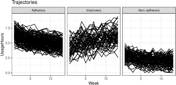
Figure 1: The trajectories from the ‘PAP.adh‘ dataset, by reference group.

4.1 Specifying methods

We first specify the methods to be evaluated. The first method of interest in this case study is KmL, selected for its flexibility in identifying patterns of any shape. The KmL method is available in the framework through the lcMethodKML class, which serves as a wrapper around the kml() function of the kml package (Genolini et al.,, 2015). The KmL method is specified through the lcMethodKML() constructor function.

kmlMethod <- lcMethodKML(response = "UsageHours", nClusters = 2)

kmlMethod

## lcMethodKML specifying "longitudinal k-means (KML)"
##  time:           getOption("latrend.time")
##  id:             getOption("latrend.id")
##  nClusters:      2
##  nbRedrawing:    20
##  maxIt:          200
##  imputationMethod:"copyMean"
##  distanceName:   "euclidean"
##  power:          2
##  distance:       function() {}
##  centerMethod:   meanNA
##  startingCond:   "nearlyAll"
##  nbCriterion:    1000
##  scale:          TRUE
##  response:       "UsageHours"

Note that any unspecified arguments have been set to the default values defined by the kml package. The method arguments can be accessed using the $ or [[ operator. Requested arguments are evaluated unless disabled by the argument eval = FALSE. As can be seen in the method output below, the time index column is obtained from the options mechanism by default.

kmlMethod$time

## [1] "Week"

kmlMethod[["time", eval = FALSE]]

## getOption("latrend.time")

Next, we specify the other methods of interest. We use a variety of approaches that are applicable to this type of data. We evaluate a feature-based approach based on LMKM as implemented in lcMethodLMKM, a distance-based dynamic time warping approach via lcMethodDtwclust based on the dtwclust package, and the regression-based approaches via the lcMethodLcmmGBTM and lcMethodLcmmGMM methods based on the lcmm package (Proust-Lima et al.,, 2017). We specify the distance-based approach using dynamic time warping. For LMKM, GBTM and GMM, we model the trajectories using an intercept and slope. Moreover, GBTM and GMM are specified to use a shared diagonal variance-covariance matrix. The GMM defines a random patient intercept.

dtwMethod <- lcMethodDtwclust(response = "UsageHours", distance = "dtw_basic")

lmkmMethod <- lcMethodLMKM(formula = UsageHours ~ Week)

gbtmMethod <- lcMethodLcmmGBTM(fixed = UsageHours ~ Week,

  mixture = ~ Week, idiag = TRUE)

gmmMethod <- lcMethodLcmmGMM(fixed = UsageHours ~ Week,

  mixture = ~ Week, random = ~ 1, idiag = TRUE)

The method arguments of a lcMethod object cannot be modified. Instead, a new specification is created from the existing one with the updated method arguments. Any lcMethod object can be used as a prototype for creating a new specification with new, modified, or removed arguments using the update() function. As an example, if we would like to respecify KmL to identify three clusters, this can be done by updating the existing specification as follows:

kml3Method <- update(kmlMethod, nClusters = 3)

As the number of clusters is generally not known in advance, we need to fit the methods for a range of number of clusters. Generating specifications for a series of argument values can be done via the lcMethods() function, which outputs a list of updated lcMethod objects from a given prototype. We specify each method for up to six clusters using:

kmlMethods  <- lcMethods(kmlMethod,  nClusters = 1:6)

lmkmMethods <- lcMethods(lmkmMethod, nClusters = 1:6)

dtwMethods  <- lcMethods(dtwMethod,  nClusters = 2:6)

gbtmMethods <- lcMethods(gbtmMethod, nClusters = 1:4)

gmmMethods  <- lcMethods(gmmMethod,  nClusters = 1:4)

length(gmmMethods)

## [1] 4

4.2 Fitting methods

Using the previously created method specifications, we can estimate the methods for the PAP.adh data. For estimating a single method, we can use the latrend() function. The function optionally accepts an environment through the envir argument for evaluating the method arguments within a specific environment. The output of the function is the fitted lcModel object.

lmkm2 <- latrend(lmkmMethod, data = PAP.adh)

summary(lmkm2)

## Longitudinal cluster model using lmkm
## lcMethodLMKM specifying "lm-kmeans"
##  time:           "Week"
##  id:             "Patient"
##  nClusters:      2
##  center:         ‘meanNA‘
##  standardize:    ‘scale‘
##  method:         "qr"
##  model:          TRUE
##  y:              FALSE
##  qr:             TRUE
##  singular.ok:    TRUE
##  contrasts:      NULL
##  iter.max:       10
##  nstart:         1
##  algorithm:      ‘c("Hartigan-Wong", "Lloyd", "Forgy", "M
##  formula:        UsageHours ~ Week
##
## Cluster sizes (K=2):
##           A           B
## 135 (44.9%) 166 (55.1%)
##
## Number of obs: 3913, strata (Patient): 301
##
## Scaled residuals:
##     Min.  1st Qu.   Median     Mean  3rd Qu.     Max.
## -2.52815 -0.67127 -0.06772  0.00000  0.54587  4.04438

Instead of needing to update a method prior to calling latrend(), the arguments to be updated can also be passed directly to latrend(). Here, we estimate the LMKM method for three clusters.

lmkm3 <- latrend(lmkmMethod, nClusters = 3, data = PAP.adh)

Alternatively, we can achieve the same result by updating the previously estimated two-cluster solution.

lmkm3 <- update(lmkm2, nClusters = 3)

4.2.1 Batch estimation

The latrendBatch() function estimates a list of method specifications. This is useful for evaluating a method for a range of number of clusters, as we have defined above using the lcMethods() function. Another use case is the improvement of model convergence and the estimation time by tuning the control parameters. Optimizing such parameters may yield considerably improved convergence or considerably reduced estimation time on larger datasets. Many of the methods have settings for the number of random starts, maximum number of iterations, and convergence criteria. However, because such control settings are specific to each method, we will not cover this.

The inputs to the latrendBatch() function are a list of lcMethod objects, and a list of datasets. The output is an lcModels object, representing a list of the fitted lcModel objects for each dataset. A seed is specified to ensure reproducibility of the examples.

lmkmList <- latrendBatch(lmkmMethods, data = PAP.adh, seed = 1)

lmkmList

## List of 6 lcModels with
##   .name .method       seed nClusters
## 1     1    lmkm  762473831         1
## 2     2    lmkm 1762587819         2
## 3     3    lmkm 1463113723         3
## 4     4    lmkm 1531473323         4
## 5     5    lmkm 1922000657         5
## 6     6    lmkm 1985277999         6

When printing a lcModels object, the content is shown as a table of method specifications. By default, only arguments which differ between the models are shown. The table can also be obtained as a data.frame by calling as.data.frame(). We now fit the other methods in the same manner.

dtwList <- latrendBatch(dtwMethods, data = PAP.adh, seed = 1)

For the repeated estimation of more computationally intensive methods, we can speed up the process by using parallel computation. By setting parallel = TRUE, the latrendBatch() function will use the parallel back-end of the foreach package (Microsoft and Weston,, 2022). To make use of this functionality, we first need to configure the parallel back-end:

nCores <- parallel::detectCores(logical = FALSE)

if (.Platform$OS.type == "windows") {

  doParallel::registerDoParallel(parallel::makeCluster(nCores))

} else {

  doMC::registerDoMC(nCores)

}

The methods can then be estimated in parallel using:

kmlList  <- latrendBatch(kmlMethods,

  data = PAP.adh, parallel = TRUE, seed = 1)

gbtmList <- latrendBatch(gbtmMethods,

  data = PAP.adh, parallel = TRUE, seed = 1)

gmmList  <- latrendBatch(gmmMethods,

  data = PAP.adh, parallel = TRUE, seed = 1)

4.3 Evaluation

4.3.1 Assessing a cluster result

A cluster result is useful only when it describes the data adequately. There are various aspects on which the cluster result can be evaluated, depending on the method and analysis domain:

• The identified solution may not be reliable when the method estimation procedure did not converge. Convergence can be checked via the converged() function.

• The cluster solution may comprise empty clusters or clusters with a negligible proportion of trajectories. In such case, re-estimating the method may yield a better solution. Alternatively, one should consider fitting the method with a lower number of clusters.

• The cluster trajectories may be assessed visually to determine whether the identified patterns are sufficiently distinct.

• The prediction error may help to determine to which degree trajectories are represented by one of the clusters.

As shown in the previous section, the summary of an lcModel object shows the method arguments values, cluster sizes, cluster proportions, cluster names, and the standardized residuals. By default, the residuals are computed from the difference between the reference values and the predictions outputted by fitted(), conditional on the most likely trajectory assignments. For methods that do not provide trajectory-specific predictions, the fitted values are determined from the cluster trajectories.

The cluster trajectories can be obtained using the clusterTrajectories() function, returning a data.frame. The cluster trajectories can be plotted via plot() or plotClusterTrajectories(). The three-cluster LMKM solution is visualized in Figure 2. For parametric cluster methods, a more concise representation of the model can be obtained from the model coefficients, using coef().

plot(lmkm3, size = 1)

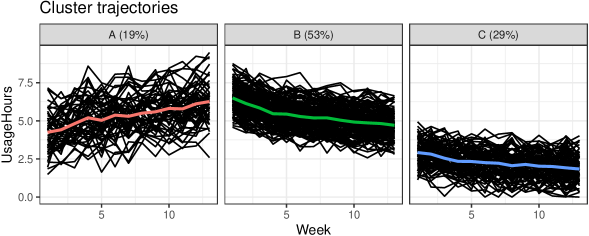
Figure 2: The cluster trajectories of the three-cluster solution identified by LMKM, created using ‘plot(lmkm2)‘.

Assigning descriptive names to the clusters can help to increase the readability of the cluster result, which is especially useful for solutions with many clusters. The clusterNames() function can be used to retrieve or change the cluster names.

clusterNames(lmkm3) <- c("Struggling", "Increasing", "Decreasing")

The most likely cluster for each of the trajectories is obtained using the trajectoryAssignments() function, which outputs a factor with the cluster names as its levels. For soft-cluster representations, the cluster assignments are determined by the cluster with the highest probability, based on the posterior probability matrix. An alternative approach can be specified through the strategy argument. For example, the which.weight() function assigns a random cluster weighted by the proportions. The which.is.max() function from the nnet package (Venables and Ripley,, 2002) returns the most likely cluster, breaking ties at random.

The posterior probability matrix can be obtained from the postprob() function. For probabilistic methods, it can be used to gauge the cluster separation, i.e., the certainty of assignment. The posterior probability is also important in the post-hoc analysis for accounting for the uncertainty in cluster assignment.

When it comes to longitudinal representation, the minimum functionality that is available for all lcModel objects is the prediction of the cluster trajectories at the given moments in time. The prediction has been implemented for underlying packages that lack this functionality. For non-parametric methods such as KmL or LLPA, linear interpolation is used when time points are requested which are not represented by the cluster centers.The available functionality differs between methods.

All lcModel objects support the standard model functions from the standard stats package, including fitted(), residuals(), and predict(). These functions are primarily of interest for methods that have a notion of a group or individual trajectory prediction error, such as for the regression-based approaches like GBTM and GMM. The fitted() function returns the expected values for the response variable for the data on which the model was estimated. By default, only the values for the most likely cluster are given. However, for clusters = NULL, a matrix of predictions is outputted, where each column represents the predictions of the respective cluster.

The predict() function computes trajectory- and cluster-specific predictions for the given input data.

predict(lmkm3, newdata = data.frame(Week = c(1, 10), Cluster = "Decreasing"))

##        Fit
## 1 2.919423
## 2 2.024865

The predictPostprob() and predictAssignments() functions compute the posterior probability and cluster membership for new trajectories, respectively. As this is not a common use case for cluster methods, most of the underlying packages do not provide this functionality. For demonstration purposes, we have implemented the functionality for the lcModelKML class.

Using the metric interface defined in Section 2, we can compute a variety of internal metrics through the metric() function:

metric(lmkm3, c("MAE", "RMSE", "Dunn", "ASW"))

##        MAE       RMSE       Dunn        ASW
## 0.74262252 0.94094913 0.09173111 0.35605235

With a regression-based approach, another aspect that is worthwhile to assess are the residuals of the predicted values. This can be investigated, for example, through a visual inspection using a quantile-quantile (Q-Q) plot, available via the qqPlot() function, to assess whether the prediction errors approximately follow a normal distribution.

4.3.2 Identifying the number of clusters

Using one or more internal metrics of interest, we can assess how the data representation of a method improves or worsens for an increasing number of clusters. In this case study, we will use the Dunn index as the primary metric for the choice of the number of clusters.

The change in metrics for an increasing number of clusters can be visualized via the plotMetric() function, and can help to determine the preferred solution. For brevity, we will only provide a detailed view for the KmL method. We plot the Dunn index, WMAE, and estimation time (in seconds) for the six KmL solutions as follows:

plotMetric(kmlList, c("Dunn", "WMAE", "estimationTime"))

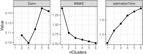
Figure 3: The Dunn index (higher is better), and WMAE (lower is better) metrics for each of the KmL solutions from 1 to 6 clusters

The resulting plot is shown in Figure 3. The Dunn index and WMAE show a rather convincing improvement for an increasing number of clusters.

Moreover, we observe that the estimation time increases with the number of clusters. This can be a practical consideration when deciding on the preferred method to use. For much larger datasets, it may be useful to conduct a preliminary analysis on a subset of the data for possibly ruling out methods which are too computationally intensive in relation to the results.

We can obtain the metric values for each of the models by calling the metric() function.

metric(kmlList, c("Dunn", "WMAE", "estimationTime"))

##         Dunn      WMAE estimationTime
## 1         NA 1.4261264           0.70
## 2 0.10737225 0.7850566           1.13
## 3 0.09944419 0.6523208           1.37
## 4 0.11353357 0.6081128           1.65
## 5 0.13487175 0.5619086           1.79
## 6 0.13196444 0.5197172           1.90

As the preferred solution corresponds to the highest Dunn index, we can obtain the respective model by calling the max() function on the lcModels list object.

kmlBest <- max(kmlList, "Dunn")

Alternatively, we can select the preferred model using the subset() function. By specifying the drop = TRUE, the lcModel object is returned instead of a lcModels object.

kmlBest <- subset(kmlList, nClusters == 5, drop = TRUE)

The identification of the number of clusters is a form of model selection. The same approach can therefore be used for identifying the best cluster representation, e.g., evaluating different formulas for a parametric model, or selecting a different method initialization strategy.

4.3.3 Comparing methods

The optimal number of clusters according to the internal metric can be different for other methods or specifications thereof. Depending on the cluster representation, some methods may require fewer or more clusters to represent the heterogeneity to the same degree. By concatenating the lists of fitted methods, we can create a metric plot that is grouped by the type of method as follows:

allList <- lcModels(lmkmList, kmlList, dtwList, gbtmList, gmmList)

plotMetric(allList, name = c("Dunn", "WMAE", "BIC", "estimationTime"), group = '.method')

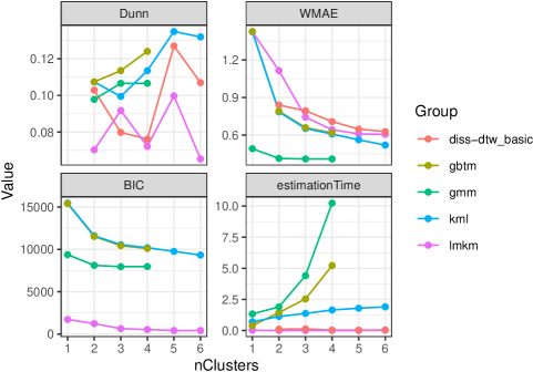
Figure 4: The Dunn index (higher is better), WMAE (lower is better) and BIC (relatively lower is better) for each of the methods and number of clusters

The WMAE and BIC between GBTM and KmL are almost exactly the same, possibly indicating that the methods find a similar solution. If the solutions are found to be practically identical, then one could actually prefer KmL due to its considerably favorable computational scaling with the number of clusters.

We explore the best solution of each method further to better understand how the cluster representations differ between the methods. We can select the preferred lcModel object corresponding to the selected number of clusters for each of the methods using the subset() function.

kmlBest  <- subset(kmlList,  nClusters == 5, drop = TRUE)

dtwBest  <- subset(dtwList,  nClusters == 5, drop = TRUE)

gbtmBest <- subset(lmkmList, nClusters == 4, drop = TRUE)

lmkmBest <- subset(lmkmList, nClusters == 3, drop = TRUE)

gmmBest  <- subset(gmmList,  nClusters == 3, drop = TRUE)

We can then assess the pairwise ARI between each method using the externalMetric() function. Calling this function on a lcModels list returns a dist object representing a distance matrix. We therefore create a list of the best lcModel for each method, by which we can then determine the pairwise ARI as follows:

bestList <- lcModels(KmL = kmlBest, DTW = dtwBest,

  LMKM = lmkmBest, GBTM = gbtmBest, GMM = gmmBest)

externalMetric(bestList, name = "adjustedRand") |> signif(2)

##       KmL  DTW LMKM GBTM
## DTW  0.39
## LMKM 0.48 0.40
## GBTM 0.65 0.31 0.67
## GMM  0.49 0.40 0.99 0.68

With all pairwise ARI being at least 0.31, all methods demonstrate some degree of similarity between each other. In particular, the very high ARI of approximately 0.99 between GMM and LMKM implies that the methods grouped the trajectories in a highly similar way.

Secondly, we compare the similarity of the cluster trajectories between the methods using the WMMAE. The easiest way to compare methods is to compare the cluster trajectories visually. However, this approach is only practical on smaller datasets or solutions with few clusters. As a more scalable alternative, we can use external metrics to measure the pairwise similarity between the cluster trajectories of the methods.

externalMetric(bestList, name = "WMMAE") |> signif(2)

##        KmL   DTW  LMKM  GBTM
## DTW  0.100
## LMKM 0.140 0.130
## GBTM 0.068 0.130 0.091
## GMM  0.130 0.130 0.036 0.099

The mean absolute error of 0.091 between the cluster trajectories of GBTM and LMKM is negligible compared to the residual error estimated by GBTM ($\textrm{SD}=0.8$), which indicates that both methods have identified practically the same cluster trajectories. The same applies to GMM and LMKM.

4.4 Cluster validation

Assessing the stability and reproducibility of a cluster method can help to determine whether the identified cluster solution generalizes beyond the data that was used to estimate the method. This is especially relevant for more complex cluster methods involving many parameters, which may not generalize well to new data. This primarily pertains to the number of clusters the method is estimated for, as the number of parameters increases linearly with the number of clusters. Even relatively simple methods can overfit the data when the representation comprises too many clusters in relation to the sample size.

4.4.1 Cluster stability using repeated estimation

Many of the cluster methods can yield a slightly different solution during each run, depending on the starting conditions. In such cases, by doing a repeated estimation, we can gauge the stability, i.e., consistency, of the method. Comparing repeated estimation results is also useful for selecting the best solution for a given method.

Repeated estimation can be done via the latrendRep() function, where the number of repetitions is specified via the .rep argument. Similar to latrend(), the method arguments can be updated within the function. The function returns a lcModels object, comprising a list of lcModel objects. Here, we only use five repeated estimations to limit the computation time. In practice, a higher number such as 10 or 25 is advisable, depending on the magnitude of instability.

kmlRepList <- latrendRep(kmlMethod, data = PAP.adh,

  nClusters = 5, .rep = 5, .parallel = TRUE)

summary(metric(kmlRepList, c("Dunn", "WMAE")))

##       Dunn             WMAE
##  Min.   :0.1047   Min.   :0.5599
##  1st Qu.:0.1349   1st Qu.:0.5610
##  Median :0.1349   Median :0.5617
##  Mean   :0.1288   Mean   :0.5618
##  3rd Qu.:0.1349   3rd Qu.:0.5619
##  Max.   :0.1349   Max.   :0.5647

The result suggests that the solutions found by KmL for the given number of clusters has some degree of variability, which could indicate that different solutions are found for the same number of clusters.

4.4.2 Cluster stability using bootstrap sampling

Instead of assessing the cluster stability across repeated estimation on the same dataset, we can obtain a more generalizable estimate of the cluster stability by measuring the cluster stability across different datasets. Bootstrap sampling, also referred to as bootstrapping, involves the repeated estimation on simulated datasets generated from the original dataset. It is primarily used for assessing the stability of a method, as measured by one or more internal metrics. Here, complete trajectories are selected at random with replacement from the dataset to generate a new dataset of equal size. Each simulated dataset, referred to as a bootstrap sample in this context, will yield a slightly different solution. This variability between samples can provide an indication of the stability of the cluster method on the overall dataset (Hennig,, 2007). Since the repeated estimation is done on new datasets that only partially overlap, this restricts the available external metrics to only those that can compare between different datasets, e.g., the WMMAE.

The latrendBoot() function applies bootstrapping to the given method specification. The samples argument determines the number of times the data is resampled, and a model is estimated. Setting the seed argument ensures that the same sequence of bootstrap samples is generated when redoing the bootstrapping procedure. The output is a lcModels list containing the model for each sample. The estimated methods each have a different call for the data argument such that the original bootstrap training sample can be recreated as needed. This avoids the need for models to store the training data. As an example, we compute 20 bootstrap samples (i.e., repeated fits) in parallel as follows:

kmlMethodBest <- update(kmlMethod, nClusters = 5)

kmlBootModels <- latrendBoot(kmlMethodBest, data = PAP.adh,

  samples = 10, seed = 1, parallel = TRUE)

head(kmlBootModels, n = 3)

## List of 3 lcModels with
##   .name .method                                        data       seed
## 1     1     kml  bootSample(PAP.adh, "Patient", 762473831L) 1062140483
## 2     2     kml bootSample(PAP.adh, "Patient", 1762587819L)  185557490
## 3     3     kml bootSample(PAP.adh, "Patient", 1463113723L)  934902099

We can now assess the stability of the solutions across the models in terms of metrics of interest. Here, we assess the mean convergence rate, and the quantiles of the WMAE and Dunn metrics.

bootMetrics <- metric(kmlBootModels, c("converged", "Dunn", "WMAE"))

mean(bootMetrics$converged)

## [1] 1

summary(bootMetrics$Dunn)

##    Min. 1st Qu.  Median    Mean 3rd Qu.    Max.
##  0.1351  0.1477  0.1506  0.1570  0.1688  0.1852

summary(bootMetrics$WMAE)

##    Min. 1st Qu.  Median    Mean 3rd Qu.    Max.
##  0.5289  0.5490  0.5553  0.5534  0.5587  0.5736

As can be seen from the output, there is quite some variability between the estimated solutions across bootstrap samples. This suggests that we should consider estimation with repeated random starts to identify a better and more stable solution.

Lastly, we can compute a similarity matrix for an external metric of interest, containing the pairwise similarity for each model pair.

wmmaeDist <- externalMetric(kmlBootModels[1:10], name = "WMMAE")

summary(wmmaeDist)

##    Min. 1st Qu.  Median    Mean 3rd Qu.    Max.
## 0.01392 0.06029 0.07294 0.06841 0.07934 0.11060

Showing that there is only a small degree of discrepancy in the cluster trajectories between bootstrap samples.

4.4.3 Comparison to ground truth

We now consider the case where a method is evaluated in a simulation study. In such a study, the ground truth is known, and we can directly evaluate whether the trajectories are clustered correctly. A useful and intuitive measure is the split-join distance (Van Dongen,, 2000), which is an edit distance that measures the number of trajectory reassignments that are needed to go from one partitioning to another. In case of a ground truth, we are only interested in the edit distance from the reference partitioning.

We can obtain the vector of trajectory cluster membership of the PAP.adh from the Group column by selecting the first cluster name of each trajectory, since the cluster membership is stable over time. We then create a lcModelPartition from the computed membership vector. By default, the lcModelPartition generates the cluster representations from the means of the trajectories assigned to the respective cluster.

refAssignments <- aggregate(Group ~ Patient, data = PAP.adh, FUN = head, n = 1L)

refAssignments$Cluster = refAssignments$Group

refModel <- lcModelPartition(data = PAP.adh,

  trajectoryAssignments = refAssignments, response = "UsageHours")

refModel

## Longitudinal cluster model using part
## lcMethod specifying "undefined"
## no arguments
##
## Cluster sizes (K=3):
##     Adherers    Improvers Non-adherers
##  162 (53.8%)   56 (18.6%)   83 (27.6%)
##
## Number of obs: 3913, strata (Patient): 301
##
## Scaled residuals:
##      Min.   1st Qu.    Median      Mean   3rd Qu.      Max.
## -3.894748 -0.643670 -0.009533  0.000000  0.634893  3.590377

We can now compare our selected method solutions to the reference solution using the one-way split-join distance to the reference:

externalMetric(bestList, refModel, name = "splitJoin.ref", drop = FALSE)

##      splitJoin.ref
## KmL             24
## DTW             61
## LMKM             3
## GBTM             1
## GMM              2

This shows that, for the PAP.adh dataset, LMKM, GBTM, and GMM achieve a nearly perfect recovery of the cluster memberships, but that GBTM needs more clusters to represent the dataset.

5 Implementing new methods

One of the main strengths of the framework is the standard way in which methods are specified, estimated, and evaluated. These aspects make it easy to compare newly implemented methods with existing ones. Using the base classes lcMethod and lcModel, new methods can be implemented with a relatively minimal amount of code, enabling rapid prototyping. These classes provide basic functionality, from which the user can extend certain functions as needed by creating a subclass.

5.1 Stratification

The simplest form of clustering is the stratification of the dataset based on a known factor. This can be the response variable, or any other measure available for each trajectory. This is useful for case studies where there is prior knowledge or expert guidance on how the trajectories should be grouped; either by another factor (e.g., age or gender), or a characteristic of the trajectory (e.g., the intercept, slope, average, or variance).

A stratification approach can be specified using the lcMethodStratify() function, which takes an R expression as input. The expression is evaluated within the data.frame at the trajectory level during the method estimation, so any column present in the data can be used. The expression should resolve to a number or category, indicating the stratum for the respective trajectory.

As an example, we stratify the trajectories by thresholding on the mean hours of usage. This expression returns a logical value which determines the cluster assignment. For categorizing trajectories into more than two clusters, the cut() function can be used. The cluster trajectories are computed by aggregating the trajectories of each cluster at the respective time points. By default, the average is computed, but an alternative center function can be specified via the center argument.

stratMethod <- lcMethodStratify(response = "UsageHours", stratify = mean(UsageHours) > 4)

stratModel <- latrend(stratMethod, data = PAP.adh)

clusterProportions(stratModel)

##         A         B
## 0.3156146 0.6843854

5.2 Feature-based clustering

Feature-based clustering is a flexible and fast approach to clustering longitudinal data, with an essentially limitless choice of trajectory representations. The framework includes a generic feature-based clustering class named lcMethodFeature for quickly implementing this approach.

A lcMethodFeature specification requires two functions: A representation function outputting the trajectory representation matrix, and a cluster function that applies a cluster algorithm to the matrix, returning an lcModel object.

To illustrate the method, we represent each trajectory using a linear model, and we cluster the model coefficients using $k$-means. In the representation step, lm() is applied to each trajectory, and the model coefficients are combined into a matrix with the trajectory-specific coefficients on each row. We parameterize the lcMethod implementation by obtaining the model formula from method$formula. During the method specification, the user therefore needs to define the formula argument. The representation function is as follows:

repStep <- function(method, data, verbose) {

  repTraj <- function(trajData) {

    lm.rep <- lm(method$formula, data = trajData)

    coef(lm.rep)

  }

  dt <- as.data.table(data)

  coefData <- dt[, as.list(repTraj(.SD)), keyby = c(method$id)]

  coefMat <- as.matrix(subset(coefData, select = -1))

  rownames(coefMat) <- coefData[[method$id]]

  coefMat

}

We implement the cluster step to return a lcModelPartition object based on the cluster assignments outputted by kmeans(). We have parameterized the function by obtaining the number of clusters for $k$-means from the nClusters model argument. The cluster function is as follows:

clusStep <- function(method, data, repMat, envir, verbose) {

  km <- kmeans(repMat, centers = method$nClusters)

  lcModelPartition(response = responseVariable(method), method = method,

    data = data, trajectoryAssignments = km$cluster, center = mean)

}

We can now specify and estimate the feature-based method, including the additionally required arguments. Comparing the estimated model to the preferred KmL model, we see that the solutions have a relatively high degree of overlap.

tsMethod <- lcMethodFeature(response = "UsageHours", formula = UsageHours ~ Week,

  representationStep = repStep, clusterStep = clusStep)

tsModel <- latrend(tsMethod, data = PAP.adh, nClusters = 5)

externalMetric(tsModel, kmlBest, "adjustedRand")

## adjustedRand
##    0.4487578

externalMetric(tsModel, kmlBest, "WMMAE")

##      WMMAE
## 0.08127578

5.3 Implementing a method

The framework is designed to support the implementation of new methods, so that users can extend or implement new methods to address their use case. In this section, we describe the high-level steps that are involved in adding support for a method to the framework. Considering the number of lines of code for even a relatively simple cluster method, we do not cover a complete example here. Instead, we only outline the typical set of functions (fit(), getArgumentDefaults(), getName(), getShortName()) that need to be implemented, together with any relevant input and output assumptions of these functions. For complete examples, see the lcMethod-interface implementations based on external packages, e.g., lcMethodKML or lcMethodLcmmGMM. A step-by-step example of implementing a statistical method in the framework can be found in the vignette included with the package, which can be viewed by running vignette("implement", package =  "latrend").

The estimation process of a method is divided into six steps, involving the processing of the method arguments, preparing and validating the data, and fitting the specified method. All steps except for fit() are optional.

1. The prepareData() function transforms the training data into the required format for the internal method estimation code. By default, data is provided in long format in a data.frame. For most implementations, no transformation is therefore needed. Cluster methods for repeated-measures data typically require data to be transformed to matrix format, however.

2. The compose() function evaluates the method arguments and returns an updated lcMethod object with the evaluated method arguments. The function can also be used for modifying or even replacing the original lcMethod object for the remainder of the estimation process. This is useful when a method is a special case of a more general method and intends to conceal derivative or redundant arguments from the base class.

3. The validate() function enables evaluated method arguments to be checked against the input data. This can be used, for example, for checking whether the data contains the covariates specified in the method formula, or whether an argument has a valid value. For implementations which wrap an underlying package function, this validation is usually not needed as the underlying package already performs validation of the input.

4. The preFit() function is intended for processing any arguments prior to fitting. In order for these results to be persistent, they should be returned in an environment object, which will be passed as an input to the fit() function.

5. The fit() function is where the internal method is estimated for the given specification to obtain the cluster result. This function is also responsible for creating the corresponding lcModel object. The running time of this function is used to determine the method estimation time.

6. The postFit() function takes the outputted lcModel from fit() as input, enabling post-processing to be done. This is used, for example, for computing derivative statistics, or for reducing the memory footprint by stripping redundant data fields from the internal model representation. Preferably, this function is implemented such that it can be called repeatedly, allowing for updates to fitted methods without requiring re-estimation.

The implementation of a method requires defining a new lcMethod class, which we will name lcMethodExample here. Usually, a new lcModel class needs to be implemented to handle the result and representation of the fitted method, which we will name lcModelExample in the example below. If the new method only outputs a partitioning, then the lcModelPartition class may be used instead.

5.3.1 Extending the method class

Defining a new method involves creating a subclass of the lcMethod class, defining its default arguments, its name, and any logic needed for the fitting procedure.

We start by defining the lcMethodExample class.

setClass("lcMethodExample", contains = "lcMethod")

Any method can be specified by instantiating the respective class through the new() function. It is recommended to rely on the object initialization mechanism of the base lcMethod class for this, as it takes care of collecting all arguments and adding default values for missing arguments. Defining new method arguments in custom class slots would hinder users from passing specialized or new optional arguments to the underlying estimation call.

Given that the base class handles the initialization of our lcMethodExample class, all we need to do is to define the default argument values in a named list. By adding formals(stats::kmeans) to the named list, our method will inherit all arguments from the kmeans() function.

setMethod("getArgumentDefaults", "lcMethodExample", function(object) {

  c(

    formals(stats::kmeans),

    time = quote(getOption("latrend.time")),

    id = quote(getOption("latrend.id")),

    nClusters = 2,

    callNextMethod()

  )

})

Method arguments can be of any class. However, we recommend that methods are specified using scalar arguments. This results in a more easily readable method summary, and greatly simplifies the permutation of argument options in a simulation study.

For identification purposes, it is recommended to specify a name and an abbreviated name for the method. This can be done by implementing the getName() and getShortName() functions, returning the names as character.

setMethod("getName", "lcMethodExample", function(object) "simple example method")

setMethod("getShortName", "lcMethodExample", function(object) "example")

We can now specify our example method by instantiating an object through the new() function, providing optional arguments as additional inputs.

new("lcMethodExample", nClusters = 3)

## lcMethodExample specifying "simple example method"
##  iter.max:       10
##  nstart:         1
##  algorithm:      c("Hartigan-Wong", "Lloyd", "Forgy", "Ma
##  trace:          FALSE
##  time:           getOption("latrend.time")
##  id:             getOption("latrend.id")
##  nClusters:      3

At the very least, we need to define a fit() function which uses the lcMethodExample object passed via the method argument and the data to estimate the specified model. The function returns a new lcModelExample object based on the internal model.

setMethod("fit", "lcMethodExample",

  function(method, data, envir, verbose, ...) {

    fittedRepresentation <- CODE_HERE

    new("lcModelExample", data = data, model = fittedRepresentation,

      method = method, clusterNames = make.clusterNames(method$nClusters)

)})

In case an external estimation function should be called with the defined method arguments, one can apply as.list() to the lcMethod object to obtain a named list of argument values. The external function can then be called using do.call().

Checking for missing arguments and for the correct argument type or valid values avoids late and confusing errors during the estimation process. It is therefore recommended to implement a validation mechanism of the method specification. This can be done by assigning a validation function to the class via setValidity() as part of the S4 system, or by implementing validate(). The latter function allows for easier validation as all arguments are already evaluated, and the arguments can be validated against the input data.

5.3.2 Extending the model class

We begin by defining the lcModelExample class. One can consider adding slots for representing, for example, the representational coefficients.

setClass("lcModelExample", contains = "lcModel")

The postprob() function is used to determine the cluster assignments and cluster proportions, so every lcModel subclass should provide it. In case of hard-cluster models, the posterior probability consists of zeros and ones.

setMethod("postprob", "lcModelExample", function(object) {

  ppMatrix <- CODE_HERE

  colnames(ppMatrix) <- clusterNames(object)

  return (ppMatrix)

})

The predict.lcModel() function is relatively complex due to the different types of inputs and outputs it supports. As these cases generalize across methods, the lcModel class provides a suitable standard implementation. For implementing new lcModel classes, it is therefore advisable to implement the predictForCluster() function instead of predict(), as it is called by predict.lcModel(). This function should provide a prediction for each row of the data.frame of the newdata argument, conditional on the given cluster membership.

setMethod("predictForCluster", "lcModelExample",

  function(object, newdata, cluster, ...) {

    predData <- CODE_HERE

    return (predData)

})

Lastly, implementing the predictPostprob() function enables the model to predict the posterior probability, and correspondingly the cluster membership, for new trajectories. The output should be a matrix matching the number of rows of newdata and indicating the cluster-specific probabilities in the respective columns.

setMethod("predictPostprob", "lcModelExample",

  function(object, newdata, ...) {

    ppMat <- CODE_HERE

    colnames(ppMat) <- clusterNames(object)

    return (ppMat)

})

It is also possible to override the predictAssignments() function. However, the default function already uses the output of predictPostprob(), so overriding it is only of use for implementing a more extensive or method-specific classification strategy.

6 Summary and outlook

The latrend package facilitates the standardized yet flexible exploration of heterogeneity in longitudinal datasets, with a minimal amount of coding effort. The framework provides functionality for specifying, estimating, and assessing models for clustering longitudinal data. The package builds upon the efforts of the R community by providing an interface to the many methods for clustering longitudinal data across packages. Perhaps most importantly, the latrend package makes it easy to compare between any two cluster methods, enabling users to identify the most suitable method to their use case. To ensure transparent and reproducible research, all decisions and settings that are relevant to the analysis should be reported. A useful checklist for reporting on latent-class trajectory studies is provided by Van de Schoot et al., (2017), which is also relevant to longitudinal cluster analyses in general.

Users can implement new methods within the framework or add support for other packages, enabling rapid prototyping for the case study at hand. Additionally, the standard functionality provided by the framework also reduces the effort needed in implementing a longitudinal cluster model.

We encourage the framework to be used as a first exploratory step in clustering longitudinal data, after which the identified preferred method can then be applied directly from the original package, which typically provides special tools or options not provided by the framework. To illustrate one such limitation, consider the initialization or prior specification of a longitudinal cluster model. This is generally an important aspect of model estimation that can improve the identified model solution but is challenging to facilitate in a standardized way.

Although the package allows for the automatic comparison and selection across methods through various metrics, it is advisable to assess whether the identified cluster solution is meaningful. It is a useful practice to consider domain knowledge when evaluating the solution (Nagin,, 2005), both in the choice of metrics as well as the interpretation of the clusters. For example, in some applications, the change over time is more of interest than the mean level, and vice versa. Along similar lines, a solution comprising a very small cluster (i.e., with few subjects) provides little additional descriptive power of the heterogeneity, unless the presence of outliers is of significant interest.

The framework is currently focused towards the modeling of a single continuous response variable, whereas some of the supported cluster packages already support multitrajectory modeling. The possible support for multitrajectory modeling has been accounted for in the design of the software. Similarly, while the single response is required to be numerical, support could be added for categorical outcomes such as those used in longitudinal latent class analysis. These features are planned for a future version.

Overall, we intend the framework to bridge the different approaches to clustering longitudinal data that exist from the various areas of research. We encourage users and package developers to create interfaces for their methods, as the availability of a standard framework for performing a longitudinal cluster analysis lowers the barrier to evaluating and comparing methods for applied researchers.

Computational details

The examples and figures in this paper were obtained using R 4.3.2 (R Core Team,, 2022) with the packages latrend 1.6.0, ggplot2 3.4.4 (Wickham,, 2016), and data.table 1.15.0 (Dowle and Srinivasan,, 2020). The KmL method was estimated based on the kml 2.4.6.1 package. The distance-based method utilized the dtwclust 5.5.12 package. The GBTM and GMM analyses were performed using the lcmm 2.1.0 package, with the parallel computation achieved using the foreach 1.5.2 package (Microsoft and Weston,, 2022).

R and all packages used within the article and the latrend package are available from the Comprehensive R Archive Network (CRAN) at (https://CRAN.R-project.org).

References

- Adepeju et al., (2020) Adepeju, M., Langton, S., and Bannister, J. (2020). Akmedoids R package for generating directionally-homogeneous clusters of longitudinal data sets. Journal of Open Source Software, 5(56):2379.
- Aghabozorgi et al., (2015) Aghabozorgi, S., Shirkhorshidi, A. S., and Wah, T. Y. (2015). Time-series clustering - A decade review. Information Systems, 53:16–38.
- Arbelaitz et al., (2013) Arbelaitz, O., Gurrutxaga, I., Muguerza, J., Pérez, J. M., and Perona, I. (2013). An extensive comparative study of cluster validity indices. Pattern recognition, 46(1):243–256.
- Babbin et al., (2015) Babbin, S. F., Velicer, W. F., Aloia, M. S., and Kushida, C. A. (2015). Identifying longitudinal patterns for individuals and subgroups: An example with adherence to treatment for obstructive sleep apnea. Multivariate Behavioral Research, 50(1):91–108.
- Bates et al., (2015) Bates, D., Mächler, M., Bolker, B., and Walker, S. (2015). Fitting linear mixed-effects models using lme4. Journal of Statistical Software, 67(1):1–48.
- Benaglia et al., (2009) Benaglia, T., Chauveau, D., Hunter, D. R., and Young, D. (2009). mixtools: An R package for analyzing finite mixture models. Journal of Statistical Software, 32(6):1–29.
- Bouveyron, (2015) Bouveyron, C. (2015). funFEM: Clustering in the Discriminative Functional Subspace.
- Cayanan et al., (2019) Cayanan, E. A., Bartlett, D. J., Chapman, J. L., Hoyos, C. M., Phillips, C. L., and Grunstein, R. R. (2019). A review of psychosocial factors and personality in the treatment of obstructive sleep apnoea. European Respiratory Review, 28(152).
- De la Cruz-Mesía et al., (2008) De la Cruz-Mesía, R., Quintana, F. A., and Marshall, G. (2008). Model-based clustering for longitudinal data. Computational Statistics & Data Analysis, 52(3):1441–1457.
- (10) Den Teuling, N. G., Pauws, S. C., and Van den Heuvel, E. R. (2021a). A comparison of methods for clustering longitudinal data with slowly changing trends. Communications in Statistics - Simulation and Computation.
- (11) Den Teuling, N. G., Van den Heuvel, E. R., Aloia, M. S., and Pauws, S. C. (2021b). A latent-class heteroskedastic hurdle trajectory model: Patterns of adherence in obstructive sleep apnea patients on CPAP therapy. BMC Medical Research Methodology, 21(1):1–15.
- Desgraupes, (2018) Desgraupes, B. (2018). clusterCrit: Clustering Indices.
- Dowle and Srinivasan, (2020) Dowle, M. and Srinivasan, A. (2020). data.table: Extension of ‘data.frame’.
- Dziak et al., (2015) Dziak, J. J., Li, R., Tan, X., Shiffman, S., and Shiyko, M. P. (2015). Modeling intensive longitudinal data with mixtures of nonparametric trajectories and time-varying effects. Psychological Methods, 20(4):444–469.
- Genolini et al., (2015) Genolini, C., Alacoque, X., Sentenac, M., and Arnaud, C. (2015). kml and kml3d: R packages to cluster longitudinal data. Journal of Statistical Software, 65(4):1–34.
- Grün and Leisch, (2008) Grün, B. and Leisch, F. (2008). FlexMix version 2: Finite mixtures with concomitant variables and varying and constant parameters. Journal of Statistical Software, 28(4):1–35.
- Hamaker, (2012) Hamaker, E. L. (2012). Why researchers should think "within-person": A paradigmatic rationale. In Mehl, M. R. and Conner, T. S., editors, Handbook of Research Methods for Studying Daily Life, pages 43–61. Guilford Publications.
- Hennig, (2007) Hennig, C. (2007). Cluster-wise assessment of cluster stability. Computational Statistics & Data Analysis, 52(1):258–271.
- Hubert and Arabie, (1985) Hubert, L. and Arabie, P. (1985). Comparing partitions. Journal of Classification, 2(1):193–218.
- Komárek, (2009) Komárek, A. (2009). A new R package for Bayesian estimation of multivariate normal mixtures allowing for selection of the number of components and interval-censored data. Computational Statistics & Data Analysis, 53(12):3932–3947.
- Liao, (2005) Liao, T. W. (2005). Clustering of time series data—a survey. Pattern Recognition, 38(11):1857–1874.
- McNicholas and Murphy, (2010) McNicholas, P. D. and Murphy, T. B. (2010). Model-based clustering of longitudinal data. Canadian Journal of Statistics, 38(1):153–168.
- Microsoft and Weston, (2022) Microsoft and Weston, S. (2022). foreach: Provides Foreach Looping Construct.
- Muthén, (2004) Muthén, B. (2004). Latent variable analysis: Growth mixture modeling and related techniques for longitudinal data. In The SAGE Handbook of Quantitative Methodology for the Social Sciences, pages 346–369. SAGE Publications, Inc.
- Nagin, (2005) Nagin, D. S. (2005). Group-Based Modeling of Development. Harvard University Press, 1st edition.
- Nagin et al., (2018) Nagin, D. S., Jones, B. L., Passos, V. L., and Tremblay, R. E. (2018). Group-based multi-trajectory modeling. Statistical Methods in Medical Research, 27(7):2015–2023.
- Nielsen, (2018) Nielsen, J. D. (2018). crimCV: Group-Based Modelling of Longitudinal Data.
- Proust-Lima et al., (2017) Proust-Lima, C., Philipps, V., and Liquet, B. (2017). Estimation of extended mixed models using latent classes and latent processes: The R package lcmm. Journal of Statistical Software, 78(2):1–56.
- R Core Team, (2022) R Core Team (2022). R: A Language and Environment for Statistical Computing. R Foundation for Statistical Computing.
- Rousseeuw, (1987) Rousseeuw, P. J. (1987). Silhouettes: A graphical aid to the interpretation and validation of cluster analysis. Journal of Computational and Applied Mathematics, 20:53–65.
- Sardá-Espinosa, (2019) Sardá-Espinosa, A. (2019). Time-series clustering in R using the dtwclust package. The R Journal.
- Scrucca et al., (2016) Scrucca, L., Fop, M., Murphy, T. B., and Raftery, A. E. (2016). mclust 5: Clustering, classification and density estimation using Gaussian finite mixture models. The R Journal, 8(1):205–233.
- Van de Schoot et al., (2017) Van de Schoot, R., Sijbrandij, M., Winter, S. D., Depaoli, S., and Vermunt, J. K. (2017). The GRoLTS-checklist: Guidelines for reporting on latent trajectory studies. Structural Equation Modeling: A Multidisciplinary Journal, 24(3):451–467.
- Van der Nest et al., (2020) Van der Nest, G., Lima Passos, V., Candel, M. J., and Van Breukelen, G. J. (2020). An overview of mixture modelling for latent evolutions in longitudinal data: Modelling approaches, fit statistics and software. Advances in Life Course Research, 43:100323.
- Van Dongen, (2000) Van Dongen, S. (2000). Performance criteria for graph clustering and Markov cluster experiments. techreport INS-R0012, CWI (Centre for Mathematics and Computer Science).
- Venables and Ripley, (2002) Venables, W. N. and Ripley, B. D. (2002). Modern Applied Statistics with S. Springer-Verlag, 4th edition.
- Wickham, (2016) Wickham, H. (2016). ggplot2: Elegant Graphics for Data Analysis. Springer-Verlag New York, 2nd edition.
- Yi et al., (2022) Yi, H., Dong, X., Shang, S., Zhang, C., Xu, L., and Han, F. (2022). Identifying longitudinal patterns of CPAP treatment in OSA using growth mixture modeling: Disease characteristics and psychological determinants. Frontiers in Neurology, 13:1063461.
- You, (2018) You, K. (2018). mclustcomp: Measures for Comparing Clusters.