Cluster Categorification of Rank 2 Webs
Abstract.
The homogeneous coordinate ring of the Grassmannian has a well-known cluster structure [Sco06]. There is a categorification of this cluster structure via a category of modules for a ring due to Jensen-King-Su [JKS16], building on work of Geiss-Leclerc-Schröer [GLS08], in which cluster variables correspond to indecomposable rigid modules. We give a combinatorial description of modules that correspond to rank cluster variables by using webs. This conjecturally gives the categorification of all rank cluster variables.
1. Introduction
A central example of a cluster algebra comes from the homogeneous coordinate ring of the Grassmannians, which was first discussed by Fomin-Zelevinsky [FZ02] for the case , and then by Scott [Sco06] for . The study of these cluster algebras has led to many interesting connections between different parts of mathematics and physics.
One powerful technique in the study of cluster algebras is categorification. Geiss-Leclerc-Schröer [GLS08] and Jensen-King-Su [JKS16] developed a representation-theoretic approach to the categorification of the cluster algebra structure on the Grassmannians. In this approach, cluster variables correspond to rigid indecomposable modules in some category of modules. Mutation of cluster variables corresponds to certain exact sequences of modules. Starting from a module, one can recover the corresponding element of the cluster algebra using the cluster character formula.
Another perspective on cluster structures on Grassmannians comes from invariant theory. Cluster monomials are elements in Lusztig’s dual semi-canonical basis. Fomin-Pylyavskyy [FP16] study cluster monomials and more generally the dual semi-canonical basis through -invariant theory using the web basis introduced by Kuperberg [Kup96]. They formulate precise and bold conjectures about expressing cluster variables in terms of webs. Their conjectures were one of the motivations behind this paper.
In this paper, we relate the perspectives of categorification and invariant theory. In particular, we study a family of rank functions on the Grassmannian. We express these functions via webs, and we show that they are cluster variables. Moreover, we give a combinatorial procedure for writing down the modules that categorify these webs. We conjecture that these are in fact all the rank cluster variables on the Grassmannian, and we provide evidence for this conjecture. Our bijection between functions and modules is a natural generalization of the rank version given in [JKS16].
Let us outline the contents of this paper. In Sections 2 and 3, we give a brief introduction to rank webs and modules we work with, introduce the definitions and necessary notation. In Section 4, we construct the bijection between webs and modules via the map . We also state our main theorem (Theorem 4.3). An important conceptual ingredient of the paper is given in Section 5, where we describe certain operations on webs and modules that we call “stretching”. These operations are called stretching functions. Section 6 is devoted to proving that the webs we consider are all cluster variables. Finally, in Section 7, we begin by recalling some terminology and results from [Le19] about the cactus sequence. We explicitly write down short exact sequences of modules for the mutations in this sequence, which allows us to prove the correspondence between rank webs and modules.
Acknowledgements
This project started during the Junior Trimester Programme: New Trends in Representation Theory at the Hausdorff Institute for Mathematics in Bonn, 2020. We thank Gustavo Jasso and Jan Schröer for organising the programme, and the Hausdorff Institute for their support. Parts of this work is completed at the Cluster algebras and representation theory programme at the Isaac Newton Institute for Mathematical Sciences in 2021 (supported by EPSRC grant no EP/R014604/1). EY is supported in part by the Royal Society Wolfson Award RSWF/R1/180004.
2. Webs of Rank
A -web is a bipartite graph drawn in a disc with weights on the edges such that the sum of weights around each interior vertex is . We will be interested in -webs that are inside a disc with vertices on the boundary, all colored black, numbered to . Denote
Any -web will have some number edges ending at the boundary vertices. Let us call such edges leaves. Note that leaves can intersect each other inside the disk or on the boundary vertices. We will restrict our attention to webs such that the leaves all have weight . A boundary vertex can have multiple (or no) leaves attached to it. Any such -web gives a well-defined function on [FLL19].
For any -web with with all leaves of weight , the number of leaves is a multiple of . We will call a -web with leaves a -web (or simply a web) of rank .
In this paper, we will only consider rank and rank webs. Rank webs consist of one interior white vertex and boundary black vertices. The rank webs we consider will consist of a tree with one black vertex and three white vertices inside the disk and edges as shown below: White vertices are connected to the boundary vertices with finite number of edges.

The set has a natural cyclic structure. For any the cyclic order induces a total order , where . Let be three subsets of . We will say that they are cyclically separated if there is some such that all the elements of are less than all the elements of , which are in turn less than all the elements of in the ordering . In particular, the cyclically separated sets are disjoint.
Let be cyclically separated subsets of and let be an arbitrary (possibly empty) set disjoint from and . Suppose further that and . Then we can define a rank web as follows: The elements in , and will be the labels of boundary vertices that are leaves of the tree. The vertices in will be attached to the first white vertex; the vertices in will be attached to the second white vertex, and the vertices of will be attached to the third white vertex. Each vertex of will be attached to two white vertices, but which white vertices they are attached to inside the disk does not matter. Changing the attachments of the vertices in will give us equivalent webs, in the sense that they give the same function on the Grassmannian, see [FP16].
Denote by the set of such rank webs.
Example 2.1.
Consider the homogeneous coordinate ring . The cluster algebra structure found in this ring is of Dynkin type ; twenty-two cluster variables of which we have six frozen variables. Since all Plücker coordinates are cluster variables, we have of them. This means we have two non Plücker cluster variables in this case. They can be found using exchange relations, or skein relations on webs [FP16].

The rightmost web in Figure 2 and its rotation by one are the two rank webs which are cluster variables on .
Conjecture 2.2.
The set is the complete set of rank cluster variables on the Grassmannian .
Strong evidence for this is the work of Fraser [Fra22] which describes the full canonical basis of rank functions as webs. Among those webs, the only arborizable ones are those in . It is believed that a web must be arborizable in order to be a cluster variable [FP16]. (They conjecture this for , but we believe it has a good chance of being true for as well.) Note that the number of webs in is also precisely the cardinality of rank indecomposable modules predicted in [BBL21].
3. JKS Modules
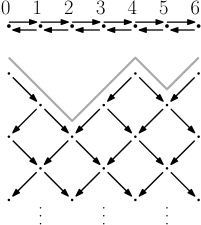
We follow the notation of Jensen-King-Su [JKS16]. Their paper gives an additive categorification of the cluster algebra structure in by using certain Cohen-Macaulay (CM) modules. We will be interested in rank and rank CM modules defined in [JKS16]. Let us give a gentle introduction to this categorification. Fix Let be a quiver as shown in Figure 3. Let be the path algebra of with the relations ‘’ and ‘’ for each vertex . We consider cyclically, so and so on. Notice that we have relations in total.

For the simplicity of the presentation, we mostly draw in a line with vertices thinking that vertices and identified (see Figure 4).
In [JKS16], they showed that rank modules are in bijection with the -subsets of which are Plücker coordinates in the corresponding Grassmannians. We use a profile for rank modules which is defined as below.
Definition 3.1.
A profile of a rank module is a series of up and down moves written respecting -subsets of as down steps and the rest of as up steps.
In Figure 4, we consider a rank module for . We describe the contours of rank modules as a sequence of ’s (up) and (down). The contour of in is
In [JKS16] they further show that every rigid indecomposable CM module has a generic filtration by rank modules. Thus we can write a profile for by superposing the profiles of rank modules in this filtration with an alignment that respects the order of the rank 1 modules in the filtration; see example below.
We will be working with the rank modules which are formed by a packing of two rank modules, denoted by . We call a profile of as in [JKS16]. We draw the contour of first and then add the contour of as close as possible to . We are “packing” the contours as close together as possible–this is necessary in order to obtain indecomposable rank modules. Examples are shown below in Figure 5.
Note that there are regions appearing between the contours in a rank module. We will call these regions “boxes” (a similar definition was given in [BBGEL22, Definition 4.1]).
Let us make this notion precise. We think of a profile as consisting of a string of length containing the letters , , , . A box of size is a string consisting of with and interspersed freely, with the restriction that it begins with and ends with .
We are interested in profiles that consist of some cyclic arrangement of three boxes with strings of and interspersed among them. For instance, a profile could be which is the first profile in Figure 5. We will see below that there is a unique indecomposable module with such a profile.
Denote the set of all such rank modules by .

Let us call and three boxes in the profile of that are divided by contours of and . Let us think of each box as consisting of a consecutive cyclic substring of . Denote and set This is to remove any common label in the profiles of and so that Set also , and . Define and respectively.
Lemma 3.2.
Let be a profile consisting of three boxes with and interspersed. Then there is a unique indecomposable module of rank with this profile. Such rank modules are the modules in .
Proof.
All the profiles we are considering have the following poset:
Thus we are looking at three lines in . There is a unique indecomposable representation of this quiver with the given dimension vectors. Up to changes of basis it is given by three different vector spaces of dimension one, which embed into a two-dimensional vector space with maps respectively. The three boxes we have in the profile are associated to the three different one-dimensional vector spaces. ∎
An alternative proof can be found in [BBL21, Theorem 1.2].
It is conjectured in [BBGE20, Conjecture 5.15] that there are rigid indecomposable rank modules corresponding to real roots. In the same paper it is shown that has at most rigid indecomposable rank modules which correspond to real roots. In [BBGEL22, Theorem 4.7], they show that there are at least
| (1) |
rigid rank indecomposable modules that correspond to roots and conjecture that this is all of them. This is precisely the number that we construct.
4. Webs and Modules
We give the recipe for translating webs into rank modules. Let us define a function
from the set of rank webs to the set of indecomposable rank modules as follows.
In a rank web, we have three white vertices inside the disk and each white vertex connected to several vertices on the boundary. As before, there will be vertices on the boundary will connect to one white vertex, vertices will connect to the second white vertex, and vertices will connect with the third white vertex. There will be vertices that are attached to any two white vertex. Set , and and solve for and . Set
-
(i)
, ,
-
(ii)
, ,
-
(iii)
, and
Here the vertices of , and are listed cyclically.
Let . Note that the and the vertices of may sit anywhere on the boundary.
Then,
where is just the listing of the elements of as , and similarly for the others.
The resulting rank module consists of three boxes: , , . These are interspersed with steps (those indices not contained in or ) and steps (those indices contained in ).
Assume , then we can visualize this map as follows (update the fig).

It is immediate from the definition of the function that the image of consists precisely of those rank modules which are three boxes (of sizes ) interspersed with and . More precisely, the image of is an indecomposable rank module.
The map is well-defined, surjective and injective; an indecomposable rank module which is formed by three boxes is uniquely determined by its profile by Lemma 3.2.
Example 4.1.
We provide a list of examples here.
![[Uncaptioned image]](/html/2402.14501/assets/x7.png)
![[Uncaptioned image]](/html/2402.14501/assets/x8.png)
![[Uncaptioned image]](/html/2402.14501/assets/x9.png)
Example 4.2.
Consider . By Equation (1), there should be rigid rank indecomposable modules.
Note that the count of the modules corresponding to real roots is corresponding to the first term in the the sum.
Now, let us count the rank webs in . We can analyze the possible values of . (Recall that , and must satisfy the triangle inequality.) The first terms counts those webs with . The second counts those with . The third counts those with or .
We may now state the main theorem of the paper:
Theorem 4.3.
If , then is a cluster variable, and the corresponding module is
5. Stretching Functions
In this section, we will define the operations of stretching (up and down) on webs and modules. These operations will give us ability to work with functions across different Grassmannians.
We begin with the stretching of modules. As a first step, consider the following function :
Definition 5.1.
Suppose with , so that defines a rank module.
-
(1)
The up stretching function takes to , where is the result of applying the map to all the indices of . In other words, and .
-
(2)
We also define the down stretching function:
We can define these functions on modules of any rank by just applying them to each contour in the profile of the module. For example, .
We have described the effect of and on the contours of a module. It is simple to see how to extend and to functors on categories of modules: Consider a module . Then is the module with for and for . The maps and are defined as before, except that is the identity map on , and is the map given by multiplication by . This is determined by the relation
Similarly, we define by for and for , but is the identity map, and is given by multiplication by .
Let us now define these up and down stretching functions for webs of rank .
Definition 5.2.
-
(1)
where .
-
(2)
where .
Example 5.3.
Here is an example of stretching of a rank web and a rank module under the up strectching map .

Stretching comes from natural maps;
If we view a point in as a matrix, the map is just forgetting the -th column. The map is the composition
where the isomorphisms come from duality.
The maps and are cluster fibrations; see [FL19, Proposition 3.4 (1)]. This means that any cluster variable on pulls back under (respectively ) to a cluster variable on (respectively ).
The following lemma shows that modules corresponding to cluster variables behave while under stretching.
Lemma 5.4.
Suppose that is an indecomposable and rigid module corresponding to a cluster variable . Then and for each are indecomposable and rigid modules corresponding to the functions and , respectively.
Proof.
The proofs for and are similar, so let us treat .
Start with a cluster for consisting of Plücker coordinates, for example, any cluster coming from a plabic graph.
For any cluster variable , will be a cluster variable on . The set can be completed to a cluster for , call this cluster . Then the quiver for the cluster is a subquiver of the quiver for . For , we know that if is the module corresponding to , then is the module corresponding to . This is because was chosen to be a Plücker coordinate.
Then we need to use the following lemma:
Lemma 5.5.
Suppose that in a cluster on . If corresponds to a module , then corresponds to the module . Let be the mutation of , having corresponding module . Then corresponds to the module .
This comes down to the fact that if we have an exact sequence
of -modules, then
is an exact sequence of of -modules. This is similarly true if and are switched. This suffices to prove the lemma.
We now return to the proof of Lemma 5.4. We have seen that if the compatibility between and holds for all the functions in the cluster , it holds for all the functions in any mutation of . Hence, by recursion, it holds for all cluster variables. ∎
6. Rank 2 webs as cluster variables
Here we show that the webs in are in fact cluster variables. First, we consider some rank webs which give functions on .
Definition 6.1.
Let be a web with and . In other words, form a partition of , and the web has exactly one leaf at each of the boundary vertices. We call such a web primitive.
Any web in comes from stretching a primitive web , see Section 5.
We previously saw that stretching a cluster variable on produces a cluster variable on or . Thus we only need to show that the primitive webs are cluster variables.
In order to do this, we use that there is a natural map
Here , where is the maximal unipotent subgroup. parameterizes complete flags in with volume forms on each subspace. The map is defined as follows. Let be the columns of the matrix representing a point of . We send this to the flags
where, for example, when we write , we mean that the -dimensional subspace of is spanned by and carries the volume form . Note that the vectors in and occur with alternative signs, so that the -form for is .
Lemma 6.2.
(see [FL19]) The cluster structure on can be pulled back from the cluster structure on . In particular, if is a cluster variable on , then is a cluster variable on .
In fact, the cluster structures on these spaces are quasi-isomorphic (isomorphic up to the frozen variables). Any cluster variable on pulls back to a cluster variable on ; the only wrinkle is that some frozen variables on become identified with a single frozen variable on .
The cluster structure on is quasi-isomorphic to the one on the double Bruhat cell (here is the longest word in the Weyl group of the Lie group ). The cluster structure on was studied extensively by Berenstein, Fomin and Zelevinsky [BFZ05] and this quasi-isomorphism is a folklore; it is implicit in Fock-Goncharov [FG06], see also [LL23].
There they show that cluster variables can be written down using the combinatorics of double reduced words. We consider the Weyl group , where we generate the first factor by simple reflections and we generate the second factor by simple reflections . One chooses a double reduced word for , which is a word in the alphabet . Corresponding to any such word is a cluster:
Theorem 6.3.
[BFZ05] Fix any reduced word for . Consider any partial word formed by the first letters of the double reduced word. The product of this partial word gives Then there exists a cluster for consisting of generalized minors where runs over such products and runs over fundamental weights.
In [LL23], Luo and the first author analyze the corresponding clusters on . Any cluster variable on has an associated quadruple of weights , which are determined by how the function transforms under the natural actions of the diagonal torus on the flags . For example, a function of weight in the flag depends on the -form on the -dimensional space of .
Proposition 6.4.
[LL23] There is a natural map such that if is a cluster variable on , then is a cluster variable on . There are cluster variables such that .
Theorem 6.5.
Note that these formulas are slightly different from those at the end of Section 6 of [LL23]; this is because our conventions and normalizations are slightly different.
Theorem 6.6.
Any primitive web in is a cluster variable.
Proof.
Consider any web with and , .
Let . Note that . Now, let us choose a double reduced word which contains as a partial word some permutation such that
There are many choices of reduced word that give rise to such and .
Then the function depends on -form from , the -form from , the -form from , and the -form from :
Invariant theory tells us that there is a unique invariant of these forms (up to scaling), which is given by the web in Figure 8.
This web is a cluster variable on which pulls back to a cluster variable on given by the web:

Up to rotation (which is a symmetry of the cluster structure), and by varying , we have exhibited all the primitive webs on as cluster variables.
∎
Corollary 6.7.
Any web in is a cluster variable.
7. Cactus sequence and Main Result
The cactus sequence is a specific sequence of mutations in the space of configurations of three flags which was studied in [Le19, Subsection 3.3]. It is a maximal green sequence on , and its tropicalization induces the Schützenberger involution. Thus it is a very natural mutation sequence to study.
Recall that is the principal flag variety for . It turns out the one can find a copy of this cluster structure “inside” (see the Lemma 7.1). Thus we can perform the cactus sequence within the cluster structure on . This sequence will allow us to access many of the rank functions on the Grassmannian. In fact, up to stretching, these functions will give us all the rank webs in .
We use that there is a natural map
The map is defined as follows. Let be the columns of the matrix representing a point of . We send this to the flags
in the notation of Section 6.
Lemma 7.1.
(see [FL19]) Let be a cluster on . Then there exists a cluster on such that . Moreover the quiver for restricts to the quiver for . Thus we can view the cluster structure on as “living inside” the cluster structure on .
The proof of Lemma 5.4 is inspired by this result, in fact we use the same idea.
Now let us define the functions appearing in the cactus sequence. Let , , . Moreover, assume that satisfy the triangle inequality. For any such we define the function on . It is determined by its pullback to the Grassmannian , . Because we will be primarily working with functions on the Grassmannian, let us simply call this pullback function as well.
Let
Definition 7.2.
Define
-
(1)
.
-
(2)
The function for and is the Plücker coordinate involving .
It is clear from the definition that the function descends to a function on .

Example 7.3.
The following webs correspond to the functions , , in . Notice that, up to the leaves intersecting, these webs are trees, so the fact that they are cluster variables in confirms the philosophy of Fomin and Pylyavskyy [FP16, Conjecture 10.1]. We can see that these functions, via stretching, can live in many Grassmanians, and they will be cluster variables thanks to Theorem 6.6.

The cactus sequence begins with a cluster that includes all of the functions for . Over the course of the mutations in the cactus sequence, one sees all of the functions of the form defined above. At the end of the sequence, one is left with the functions where , and these are the all the rank webs in , up to stretching.
The particulars of this mutation sequence, like the precise sequence of mutations and the clusters that occur along the way, are not so important for us. We will only use that each mutation which has the following form:
Proposition 7.4.
[[Le19] Proposition 3.2]
via the identity
with satisfying the appropriate inequalities for all the terms to make sense.
Some of the mutation identities will be degenerations of the above identity using one of the following identities:
Note that in Proposition 7.4, all the the mutations involve rank functions. However, we can use the degeneracy to view rank functions (Plücker coordinates) as rank functions: Thus we start with the function and mutate until we end up with the function .
For example, there is a mutation
The first and last identities are degeneracies, while the middle identity is the cactus mutation.
In the cases where
the module one would attach to the cluster variable (using a degenerate case of the procedure we described for ) is the direct sum of the modules attached to and . The analogous statement is true when
Thus these cases can be treated uniformly in the proof of Theorem 7.5 below. The final degeneracy changes the profiles of the modules in proof of Theorem 7.5, but it actually simplifies the arguments.
Because the functions in this sequence are all of the ones in , up to stretching, it is enough to understand the modules attached to the functions in this sequence. Our strategy is to use the cactus mutation sequence to recursively verify that the module corresponding to is for all the functions .
At any stage in the cactus sequence, we know the modules that categorify the cluster variables
are the ones coming from the map .
From this, we would like to compute the module which categorifies . In order to do this, we will show that satisfies the appropriate exact sequences:
Theorem 7.5.
The following are short exact sequences of modules in the categorification of :
Proof.
Recall that we may write the profile of the rank module as a stack of contours:
Thus, for example, the first exact sequence in the theorem can be written as:
Written this way, the exact sequence does not look very illuminating. Let us examine the exact sequence in a representative example, which will indicate how the general argument works. Take . In this case we get that . We are interested in the exact sequences
We wish to see these as exact sequences in . However, none of the functions involved uses the vectors or . Thus we may actually work in by eliminating and reindexing in order to make things slightly simpler. We will exhibit exact sequences of modules for the categorification of which can be stretched to give exact sequences of modules for the categorification of .
We start with the first exact sequence. Below, we picture the modules for and .
![[Uncaptioned image]](/html/2402.14501/assets/x14.png)
The regions of the diagram are labelled by vector spaces satisfying the following:
-
•
are two dimensional spaces;
-
•
are one-dimensional spaces spanned by , respectively, such that .
-
•
are one-dimensional spaces spanned by , respectively, such that .
-
•
are one-dimensional spaces spanned by , respectively, such that .
We can now describe the map and show that it is injective. We map to the direct sum of and by mapping
-
(i)
so that ;
-
(ii)
so that ;
-
(iii)
so that ;
-
(iv)
the previous maps are compatible and determin a map .
In the following diagram, we see :
![[Uncaptioned image]](/html/2402.14501/assets/x15.png)
Now, we take the cokernel of this map . We use the following natural isomorphisms that follow from linear algebra:
-
(i)
-
(ii)
-
(iii)
-
(iv)
(Note that this list of identities contains more than we need in this particular case, but it is the complete list of identities one uses in the general case.)
From this, we obtain the following module which is the desired result:
![[Uncaptioned image]](/html/2402.14501/assets/x16.png)
The module is the rank indecomposable module that we seek, corresponding to
We can similarly check the second exact sequence. Below are the modules , and their direct sum :
![[Uncaptioned image]](/html/2402.14501/assets/x17.png)
The module includes into this direct sum via the map , defined as in the previous case:
![[Uncaptioned image]](/html/2402.14501/assets/x18.png)
Using the same identities, we see that the quotient is the module :
![[Uncaptioned image]](/html/2402.14501/assets/x19.png)
Thus once we know that the functions all correspond to the modules given by applying , we see that this is also the case for .
The general argument will use the exact same diagrams, with the proportions of various rectangles scaled appropriately. One needs to make slight modifications in the case of the degenerate exact sequences, but these sequences are actually simpler.
∎
Corollary 7.6.
The pull-back of the function from to is a cluster variable whose categorification is given by the module .
Now we return to the proof of our main result, Theorem 4.3:
Proof of Theorem 4.3.
We saw that any web in comes from stretching a primitive web in , and is thus a cluster variable (Theorem 6.6, Corollary 6.7). Any web in is also related via stretching with the functions . For the webs we know the corresponding modules (as defined in Section 4) by Theorem 7.5.
But by 5.4, we understand how stretching of functions corresponds to stretching of modules: if is the module corresponding to , this holds for any web obtained from stretching . Thus for all , is the module corresponding to .
This gives the bijection between and . ∎
References
- [BBGE20] Karin Baur, Dusko Bogdanic, and Ana Garcia Elsener. Cluster categories from Grassmannians and root combinatorics. Nagoya Math. J., 240:322–354, 2020.
- [BBGEL22] K. Baur, D. Bogdanic, A. Garcia Elsener, and J-R. Li. Rigid indecomposable modules in grassmannian cluster categories. arXiv:2011.09227v3, 2022.
- [BBL21] K. Baur, D. Bogdanic, and J-R. Li. Construction of rank 2 indecomposable modules in grassmannian cluster categories. arXiv:2011.14176v2, 2021.
- [BFZ05] Arkady Berenstein, Sergey Fomin, and Andrei Zelevinsky. Cluster algebras. III. Upper bounds and double Bruhat cells. Duke Math. J., 126(1):1–52, 2005.
- [FG06] Vladimir V Fock and Alexander B Goncharov. Cluster -varieties, amalgamation, and poisson—lie groups. Algebraic Geometry and Number Theory: In Honor of Vladimir Drinfeld’s 50th Birthday, pages 27–68, 2006.
- [FL19] Chris Fraser and Ian Le. Tropicalization of positive Grassmannians. Selecta Math. (N.S.), 25(5):Paper No. 75, 55, 2019.
- [FLL19] Chris Fraser, Thomas Lam, and Ian Le. From dimers to webs. Trans. Amer. Math. Soc., 371(9):6087–6124, 2019.
- [FP16] Sergey Fomin and Pavlo Pylyavskyy. Tensor diagrams and cluster algebras. Adv. Math., 300:717–787, 2016.
- [Fra22] C. Fraser. Webs and canonical bases in degree two. arXiv:2202.01310v1, 2022.
- [FZ02] Sergey Fomin and Andrei Zelevinsky. Cluster algebras. I. Foundations. J. Amer. Math. Soc., 15(2):497–529, 2002.
- [GLS08] Christof Geiss, Bernard Leclerc, and Jan Schröer. Preprojective algebras and cluster algebras. In Trends in representation theory of algebras and related topics, EMS Ser. Congr. Rep., pages 253–283. Eur. Math. Soc., Zürich, 2008.
- [JKS16] Bernt Tore Jensen, Alastair D. King, and Xiuping Su. A categorification of Grassmannian cluster algebras. Proc. Lond. Math. Soc. (3), 113(2):185–212, 2016.
- [Kup96] Greg Kuperberg. Spiders for rank Lie algebras. Comm. Math. Phys., 180(1):109–151, 1996.
- [Le19] Ian Le. Cluster structures on higher Teichmuller spaces for classical groups. Forum Math. Sigma, 7:Paper No. e13, 165, 2019.
- [LL23] Ian Le and Sammy Luo. Generalized minors and tensor invariants. Int. Math. Res. Not. IMRN, (16):13658–13686, 2023.
- [Sco06] Jeanne S. Scott. Grassmannians and cluster algebras. Proc. London Math. Soc. (3), 92(2):345–380, 2006.