Abstract

Imbalanced data, characterized by an unequal distribution of data points across different clusters, poses a challenge for traditional hard and fuzzy clustering algorithms, such as hard K-means (HKM, or Lloyd’s algorithm) and fuzzy K-means (FKM, or Bezdek’s algorithm). This paper introduces equilibrium K-means (EKM), a novel and simple K-means-type algorithm that alternates between just two steps, yielding significantly improved clustering results for imbalanced data by reducing the tendency of centroids to crowd together in the center of large clusters. We also present a unifying perspective for HKM, FKM, and EKM, showing they are essentially gradient descent algorithms with an explicit relationship to Newton’s method. EKM has the same time and space complexity as FKM but offers a clearer physical meaning for its membership definition. We illustrate the performance of EKM on two synthetic and ten real datasets, comparing it to various clustering algorithms, including HKM, FKM, maximum-entropy fuzzy clustering, two FKM variations designed for imbalanced data, and the Gaussian mixture model. The results demonstrate that EKM performs competitively on balanced data while significantly outperforming other techniques on imbalanced data. For high-dimensional data clustering, we demonstrate that a more discriminative representation can be obtained by mapping high-dimensional data via deep neural networks into a low-dimensional, EKM-friendly space. Deep clustering with EKM improves clustering accuracy by 35% on an imbalanced dataset derived from MNIST compared to deep clustering based on HKM.

I Introduction

Imbalanced data refers to data that is unevenly distributed across different clusters, which is prevalent in medical diagnosis, fraud detection, and anomaly detection. Learning from imbalanced data has been considered a challenge and a valuable direction [1]. While there is a considerable amount of research on supervised learning from imbalanced data, e.g., [2, 3, 4], unsupervised learning has not been as thoroughly explored, due to the unknown imbalance ratio between clusters making the task more challenging [5].

Clustering is an important unsupervised learning task involving grouping data into clusters based on similarity. K-means (KM) is the most popular clustering technique, valued for its simplicity, scalability, and effectiveness with real datasets. It is also used as an initialization method for more advanced clustering techniques, such as the Gaussian mixture model [6, 7]. KM starts with an initial set of centroids (cluster centers) and iteratively refines them to increase cluster compactness. The hard KM (HKM, or Lloyd’s algorithm) [8, 9] and fuzzy KM (FKM, or Bezdek’s algorithm) [10] are the two most representative KM algorithms. HKM assigns a data point to only one cluster, while FKM allows a data point to belong to multiple clusters with varying degrees of membership. In recent, they are also widely employed in deep learning, jointly trained with deep neural networks (DNNs) for clustering high-dimensional data, such as images [11, 12, 13, 14].

Many FKM variations have been developed to enhance its performance in different aspects. For example, the possibilistic FKM (PFKM) [15] was proposed to address the sensitivity of FKM to noise and outliers. FKM-$\sigma$ [16] was proposed to improve FKM’s performance on data points with uneven densities or non-spherical shapes in individual clusters. Fuzzy local information K-means (FLICM) [17] was designed to promote FKM’s performance in image segmentation. For more information on other FKM variants, please refer to the review paper [18].

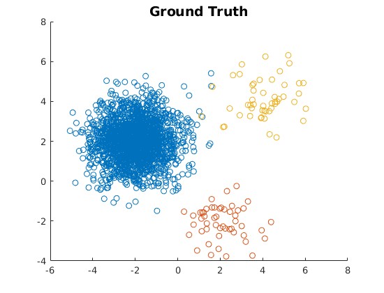
(a)

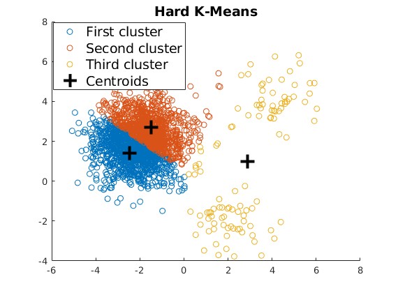
(b)

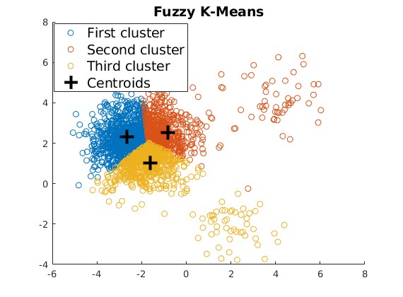
(c)

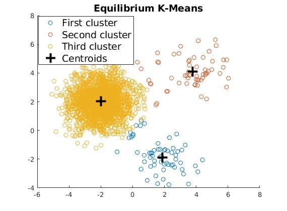
(d)

Figure 1: Clustering results of a highly imbalanced dataset. (a) Ground truth. The colors represent the labels of the data points. (b) Clustering by hard K-means. (c) Clustering by fuzzy K-means. (d) Clustering by the proposed equilibrium K-means. They are all two-step alternating algorithms that iteratively update centroids and clusters.

Clustering imbalanced data also poses a challenge for both HKM and FKM. This is due to an undesirable property known as the “uniform effect”, which causes centroids to crowd together in large clusters, resulting in clusters of equal size even when input data has varied cluster sizes. An example illustrating the uniform effect of HKM and FKM is given in Fig. 1.

I-A Existing Efforts to Overcome Uniform Effect

To improve the poor performance of FKM on imbalanced data, Noordam et al. [19] developed a modified FKM called cluster-size insensitive FKM (csiFKM). This method assigns weight to adjust the contribution of data points according to the size of the clusters they belong to. Lin et al. [20] proposed a size-insensitive integrity-based FKM (siibFKM) to reduce the sensitivity of csiFKM to the distance between adjacent clusters by increasing the cluster’s integrity. However, weighting based on cluster size inadvertently increases the influence of outliers, making these algorithms sensitive to noise [18].

Another approach to tackle the challenge of imbalanced data clustering is to use a multiprototype mechanism. This method first groups data into multiple subclusters, ensuring that the data points in each subcluster are relatively balanced. The final clusters are obtained by merging adjacent subclusters. Liang et al. [21] introduced a multiprototype clustering algorithm that employs FKM to generate subclusters. Later, Lu et al. [5] proposed a self-adaptive multiprototype clustering algorithm that can automatically adjust the number of subclusters. However, multiprototype clustering algorithms involve a complex process and high complexity, with a time complexity of $O(N^{2})$, where $N$ is the number of data points in the dataset, making them computationally expensive for large datasets. We should additionally mention that Zeng et al. [22] recently proposed a soft multiprototype clustering algorithm with time complexity linear to $N$. However, the clustering process of this algorithm remains complex and is aimed at clustering high-dimensional and complex-structured data rather than imbalanced data.

I-B Our Contributions

In this paper, we propose equilibrium K-means (EKM) for imbalanced data clustering, which avoids the limitations of the aforementioned techniques. Our contributions can be summarized in three main aspects.

First, we offer a new framework that unifies HKM, FKM, and EKM with three key advantages. 1. This framework can directly re-derive HKM and FKM from unconstrained optimization problems with differentiable objectives without applying Lagrangian multipliers, simplifying the previous derivation from constrained optimization problems and non-differentiable objectives. 2. The new objective functions of HKM and FKM can be compared in the same plot, which used to be unfeasible due to the old objective function of FKM having more optimization variables than that of HKM. Such comparison can facilitate a more comprehensive and fundamental view than existing comparisons (such as [23, 24]) based on clustering outcomes. 3. This new framework allows for the uniform study of KM-type algorithms, such as the convergence conditions provided in this paper. We also reveal an explicit relationship between these KM algorithms and Newton’s method.

Second, we present EKM, derived from the new framework. Similar to FKM, EKM is a two-step alternating algorithm between updating the weighted centroid and calculating the weight, but the membership defined in EKM has a clearer physical meaning than that defined in FKM. Besides, EKM prevents centroids crowd together by introducing appropriate repulsive forces between centroids, making it more effective than HKM and FKM on imbalanced data. In addition to having the same time and space complexity as FKM, EKM also supports batch learning, making it scalable for large datasets. We demonstrate EKM’s performance through numerical experiments on two synthetic and ten real datasets from various domains. Because of space limitations, quantified metrics of performance are presented in the supplemental material, but the scatter graphs of partial clustering outcomes that we present in the paper are sufficient to demonstrate the superiority of EKM.

Finally, we investigate the cooperation between EKM and DNNs for high-dimensional data clustering. We find that mapping high-dimensional data via DNNs to a low-dimensional EKM-friendly space results in a more discriminative representation than mapping to an HKM-friendly space. When applied to an imbalanced dataset derived from MNIST, joint learning of DNNs and EKM improves clustering accuracy by 35% compared to joint learning of DNNs and HKM.

I-C Organization

We introduce the HKM, FKM, and a variation of FKM, the maximum-entropy fuzzy clustering (MEFC) in Section II. In Section III and Section IV, we introduce the proposed clustering framework and the proposed EKM. We demonstrate the performance of EKM on classic clustering tasks in Section V and deep clustering in Section VI. Finally, we conclude in Section VII.

II K-Means and Its Variations

II-A The Hard K-Means Algorithm (Lloyd’s Algorithm)

KM clustering aims to partition $N$ data points into $K$ clusters, minimizing the sum of the variances within each cluster. Mathematically, the objective can be expressed as:

$$\underset{\mathbb{S}_{1},\cdots,\mathbb{S}_{K}}{\arg\min}\sum_{k=1}^{K}\sum_{\mathbf{x}\in\mathbb{S}_{k}}\|\mathbf{x}-\bm{\mu}_{k}\|_{2}^{2},$$ (1)

where $\mathbb{S}_{k}$ represents the set of data points in the $k$-th cluster, $\mathbf{x}\in\mathbb{S}_{k}$ denotes a data point belonging to $\mathbb{S}_{k}$, $\bm{\mu}_{k}$ is the centroid of points in $\mathbb{S}_{k}$, expressed by

$$\bm{\mu}_{k}=\frac{1}{|\mathbb{S}_{k}|}\sum_{\mathbf{x}\in\mathbb{S}_{k}}\mathbf{x},$$ (2)

$|\mathbb{S}_{k}|$ signifies the size of $\mathbb{S}_{k}$, and $\|\cdot\|_{2}$ is the $l_{2}$ norm. The optimization problem (1) is NP-hard [25], and Lloyd‘s algorithm is a popular heuristic algorithm for solving this problem. Given $K$ points ($\mathbf{c}_{1}^{(1)},\cdots,\mathbf{c}_{K}^{(1)})$ as initial centroids, Lloyd’s algorithm alternates between two steps:

1. Assign each data point to the nearest centroid, forming $K$ clusters:

   $$\mathbb{S}^{(\tau)}_{k}=\{\mathbf{x}:\|\mathbf{x}-\mathbf{c}_{k}^{(\tau)}\|_{2}^{2}\leq\|\mathbf{x}-\mathbf{c}_{i}^{(\tau)}\|_{2}^{2}\,\forall i,\,1\leq i\leq K\}$$ (3)

2. Recalculate the centroid of each cluster by taking the mean of all data points assigned to it:

   $$\mathbf{c}_{k}^{(\tau+1)}=\frac{1}{|\mathbb{S}_{k}^{(\tau)}|}\sum_{\mathbf{x}\in\mathbb{S}_{k}^{(\tau)}}\mathbf{x}.$$ (4)

Lloyd’s algorithm converges when the assignment of data points to clusters ceases to change, or when a maximum number of iterations is reached. The time complexity of one iteration of the above two steps is $O(NK)$. The HKM algorithm mentioned in this paper refers to Lloyd’s algorithm.

II-B The Uniform Effect of K-Means

The uniform effect refers to the propensity to generate clusters of equal size, which is implicitly implied in the objective (1) of KM. For simplicity, kindly consider a case with two clusters (i.e., $K=2$). Minimizing the objective function (1) is equivalent to maximizing the following objective function [26]:

$$\max_{\mathbb{S}_{1},\,\mathbb{S}_{2}}N_{1}N_{2}\|\bm{\mu}_{1}-\bm{\mu}_{2}\|_{2}^{2},$$ (5)

where $N_{1}$ and $N_{2}$ denote the sizes of $\mathbb{S}_{1}$ and $\mathbb{S}_{2}$, respectively. By isolating the effect of $\|\bm{\mu}_{1}-\bm{\mu}_{2}\|_{2}^{2}$, maximizing the above objective leads to $N_{1}=N_{2}=N/2$, indicating KM tends to produce equally sized clusters.

II-C The Fuzzy K-Means Algorithm (Bezdek’s Algorithm)

FKM attempts to minimize the sum of weighted distances between data points and centroids, with the following objective and constraints [10]:

$$\min_{\mathbf{c}_{1},\cdots,\mathbf{c}_{K},\{u_{kn}\}} \sum_{n=1}^{N}\sum_{k=1}^{K}(u_{kn})^{m}\|\mathbf{x}_{n}-\mathbf{c}_{k}\|_{2}^{2}$$ (6)

subject to $$u_{kn}\in[0,\,1]\,\forall k,n,$$

$$\sum_{k}u_{kn}=1\,\forall n,$$

$$0<\sum_{n}u_{kn}<N\,\forall k,$$

where $\mathbf{x}_{n}$ represents the $n$-th data point, $\mathbf{c}_{k}$ denotes the $k$-th centroid, $u_{kn}$ is a coefficient called membership that indicates the degree of $\mathbf{x}_{n}$ belonging to the $k$-th cluster, and $m\in(1,+\infty)$ is a hyperparameter controlling the degree of fuzziness level. Similar to the HKM algorithm, the FKM algorithm operates by alternating two steps:

1. Calculate the membership values of data points of being in the cluster:

   $$u_{kn}^{(\tau)}=\frac{1}{\sum_{i=1}^{K}\bigg{(}\frac{\|\mathbf{x}_{n}-\mathbf{c}_{k}^{(\tau)}\|_{2}}{\|\mathbf{x}_{n}-\mathbf{c}_{i}^{(\tau)}\|_{2}}\bigg{)}^{\frac{2}{m-1}}}.$$ (7)

2. Recalculate the centroid of each cluster by taking the mean of all data points, weighted by their membership to the cluster:

   $$\mathbf{c}_{k}^{(\tau+1)}=\frac{\sum_{n}(u_{kn}^{(\tau)})^{m}\mathbf{x}_{n}}{\sum_{n}(u_{kn}^{(\tau)})^{m}}.$$ (8)

The time complexity of one iteration of the above two steps is $O(NK^{2})$. The higher time complexity of FKM than that of HKM is due to the extra calculation of membership. A practical time consumption comparison can be found in [27].

II-D Maximum-Entropy Fuzzy Clustering

Karayiannis [28] added an entropy term to the objective function of FKM, resulting in MEFC. The new objective function is given as follows:

$$\min_{\mathbf{c}_{1},\cdots,\mathbf{c}_{K},\{u_{kn}\}} \eta\sum_{n=1}^{N}\sum_{k=1}^{K}u_{kn}\ln{u_{kn}}$$ (9)

$$+(1-\eta)\frac{1}{N}\sum_{n=1}^{N}\sum_{k=1}^{K}u_{kn}\|\mathbf{x}_{n}-\mathbf{c}_{k}\|_{2}^{2}$$

subject to $$u_{kn}\in[0,\,1]\,\forall k,n,$$

$$\sum_{k}u_{kn}=1\,\forall n,$$

where $\eta\in(0,1)$ is a hyperparameter, controlling the transition from maximization of the entropy to the minimization of centroid-data distances. MEFC is similar to FKM but with a different membership:

$$u^{(\tau)}_{kn}=\frac{\exp{(-\lambda\|\mathbf{x}_{n}-\mathbf{c}_{k}\|_{2}^{2})}}{\sum_{i=1}^{K}\exp{(-\lambda\|\mathbf{x}_{n}-\mathbf{c}_{i}\|_{2}^{2})}},$$ (10)

where $\lambda=\frac{1}{N}\frac{1-\eta}{\eta}$. The time complexity of MEFC is the same as FKM, which is $O(NK^{2})$ for one iteration.

III Smooth K-Means - A Unified Framework

III-A Objective of Smooth K-Means

Here, we propose a novel framework called smooth K-means (SKM) and demonstrate that the three KM algorithms introduced in the previous section are special cases of SKM. Based on this framework, we further develop a new clustering algorithm, aiming to improve the degraded performance of KM algorithms on imbalanced data. Denote the squared Euclidean distance between the $k$-th centroid and the $n$-th data point as

$$d_{kn}=\frac{1}{2}\|\mathbf{x}_{n}-\mathbf{c}_{k}\|_{2}^{2},$$ (11)

and define the within-cluster sum of squares (WCSS) as the sum of squared Euclidean distances between data points and their nearest centroid, i.e.,

$$\text{WCSS}:=\sum_{n=1}^{N}\min(d_{1n},\cdots,d_{Kn}).$$ (12)

The goal of SKM is to find $K$ centroids that minimize an approximated WCSS, resulting in the following optimization problem:

$$\underset{\mathbf{c}_{1},\cdots,\mathbf{c}_{K}}{\arg}\min\sum_{n=1}^{N}h(d_{1n},\cdots,d_{Kn}),$$ (13)

where $h(d_{1n},\cdots,d_{Kn})$ is a smooth approximation to $\min(d_{1n},\cdots,d_{Kn})$ and is referred to as the smooth minimum function. Below we explain the significance of replacing the minimum function with a smooth minimum function from a statistical point of view.

III-B Statistical Interpretation of Smooth K-Means

Statistically, the centroids obtained by minimizing WCSS are maximum likelihood estimators (MLEs) of parameters in a specific type of Gaussian mixture model (GMM) referred to as “hard” GMM. Assuming that the dataset $(\mathbf{x}_{1},\cdots,\mathbf{x}_{N})$ is generated by $K$ independent multivariate normal distributions, we denote the mean vector and covariance matrix of the $k$-th normal distribution as $\bm{\mu}_{k}$ and $\mathbf{\Sigma}_{k}$, respectively. The standard GMM assumes that data points are generated from multiple normal distributions based on a certain probability distribution, with the following likelihood

$$L(\bm{\mu},\mathbf{\Sigma},p\,|\,\mathbf{x})\propto \prod_{n=1}^{N}\sum_{k=1}^{K}p_{kn}\det(\mathbf{\Sigma}_{k})^{-1/2}$$ (14)

$$\exp{\bigl{(}-\frac{1}{2}(\mathbf{x}_{n}-\bm{\mu}_{k})^{\mathsf{T}}\mathbf{\Sigma}_{k}^{-1}(\mathbf{x}_{n}-\bm{\mu}_{k})\bigl{)}},$$

where $p_{kn}$ is the probability that the $n$-th data point is generated from the $k$-th normal distribution. The hard GMM, on the other hand, assumes that data points can only be generated from a single normal distribution. Accordingly, for all $n$, $p_{kn}=1$ for one $k\in\{1,\cdots,N\}$ and $p_{in}=0$ if $i\neq k$. We further assume that all normal distributions have the same covariance matrix, specifically an identity matrix. Under these assumptions, the MLEs of $\{p_{kn}\}$ are $\hat{p}_{kn}=1$ if $k=\arg\min_{i\in\{1,\cdots,K\}}\|\mathbf{x}_{n}-\bm{\mu}_{i}\|_{2}^{2}$, and $\hat{p}_{kn}=0$ otherwise. By substituting $\mathbf{\Sigma}_{k}=\mathbf{I}$ and $\hat{p}_{kn}$ into (14) and taking the logarithmic value, we obtain the log-likelihood:

$$l(\bm{\mu}\,|\,\mathbf{x})\propto-\sum_{n=1}^{N}\min(\|\mathbf{x}_{n}-\bm{\mu}_{1}\|_{2}^{2},\cdots,\|\mathbf{x}_{n}-\bm{\mu}_{K}\|_{2}^{2}).$$ (15)

Now it is clear that the MLEs of $\{\bm{\mu}_{1},\cdots,\bm{\mu}_{K}\}$ are the centroids minimizing WCSS.

While the hard GMM model is more computationally efficient than the standard GMM, it only considers the impact of a data point on its closest centroid. However, as seen in the success of FKM, it can be advantageous to consider the effect of data points on all centroids for certain real datasets. This can be accomplished by SKM in a parameter-free manner, which applies a smooth function to WCSS. Different smoothing methods result in unique impact patterns, allowing for the capture of various data structures. In the following sections, we will explore three popular smooth minimum functions and their impact on clustering.

III-C Three Common Smooth Minimum Functions

Assume a monotonically increasing and differentiable function $f:[0,\,+\infty)\mapsto[0,\,+\infty)$ satisfies

$$\lim_{x\to+\infty}\frac{x}{f(x)}\to 0,$$ (16)

or equivalently

$$\lim_{x\to+\infty}\frac{1}{f^{\prime}(x)}\to 0,$$ (17)

where $f^{\prime}$ is the first derivative of $f$. Let $g(x)=1/f(x)$, a smooth minimum function $h_{1}:[0,\,+\infty)^{K}\mapsto[0,+\infty)$ can be constructed by

$$h_{1}(x_{1},\cdots,x_{K})=g^{-1}(g(x_{1})+\cdots+g(x_{K}))$$ (18)

Let $f(x)$ be defined as $e^{\lambda x}$, then the function $h_{1}$ takes on a specific form known as LogSumExp:

$$h_{1}(x_{1},\cdots,x_{K}) =\text{LSE}_{\lambda}(x_{1},\cdots,x_{K})$$ (19)

$$=-\frac{1}{\lambda}\ln(e^{-\lambda x_{1}}+\cdots+e^{-\lambda x_{K}}),$$

where $\lambda$ serves as a parameter that controls the degree of approximation, with $\text{LSE}_{\lambda}\to\min$ as $\lambda\to+\infty$. Another common smooth minimum function, called p-Norm, can be defined as $f(x)=x^{p}$, which has the following specific form

$$h_{1}(x_{1},\cdots,x_{K}) =\text{PN}_{p}(x_{1},\cdots,x_{K})$$ (20)

$$=(x_{1}^{-p}+\cdots+x_{K}^{-p})^{-1/p},$$

and converges to $\min(x_{1},\cdots,x_{K})$ as $p\to+\infty$.

Smooth minimum functions can also be constructed using

$$h_{2}(x_{1},\cdots,x_{K})=\frac{x_{1}g(x_{1})+\cdots+x_{K}g(x_{K})}{g(x_{1})+\cdots+g(x_{K})}.$$ (21)

A specific example is the Boltzmann operator, which is defined as $g(x)=e^{-\alpha x}$. The Boltzmann operator takes on the form of

$$h_{2}(x_{1},\cdots,x_{K}) =\text{boltz}_{\alpha}(x_{1},\cdots,x_{K})$$ (22)

$$=\frac{\sum_{i=1}^{K}x_{i}e^{-\alpha x_{i}}}{\sum_{i=1}^{K}e^{-\alpha x_{i}}},$$

and converges to the minimum function as $\alpha\to+\infty$.

III-D Clustering by Minimizing Smoothed WCSS

III-D1 The relationship between LogSumExp and Maximum-Entropy Fuzzy Clustering

Approximating WCSS (12) by LogSumExp (19), we have the following objective:

$$\min_{\mathbf{c}_{1},\cdots,\mathbf{c}_{K}}J_{\text{LSE}}(\mathbf{c}_{1},\cdots,\mathbf{c}_{K})=\sum_{n=1}^{N}-\frac{1}{\lambda}\ln{(\sum_{k=1}^{K}e^{-\lambda d_{kn}})}.$$ (23)

The differentiable objective function $J_{\text{LSE}}$ has the first-order partial derivative:

$$\partial_{\mathbf{c}_{k}}{J_{\text{LSE}}}=\frac{\partial{J_{\text{LSE}}}}{\partial{\mathbf{c}_{k}}} =\sum_{n=1}^{N}\frac{e^{-\lambda d_{kn}}}{\sum_{i=1}^{K}e^{-\lambda d_{in}}}\frac{\partial{d_{kn}}}{\partial{\mathbf{c}_{k}}}$$ (24)

$$=-\sum_{n=1}^{N}\frac{e^{-\lambda d_{kn}}}{\sum_{i=1}^{K}e^{-\lambda d_{in}}}(\mathbf{x}_{n}-\mathbf{c}_{k}).$$

The minimizer of $J_{\text{LSE}}$ can be found by gradient descent iteration:

$$\mathbf{c}_{k}^{(\tau+1)}=\mathbf{c}_{k}^{(\tau)}-\gamma^{(\tau)}_{k}\partial_{\mathbf{c}_{k}}{J_{\text{LSE}}}(\mathbf{c}_{k}^{(\tau)}),$$ (25)

where $\gamma^{(\tau)}_{k}$ is the learning rate at the $\tau$-th iteration. This updating procedure (25) is equivalent to the MEFC algorithm if one set

$$\gamma^{(\tau)}_{k}=1/\sum_{n=1}^{N}\bigg{(}\frac{e^{-\lambda d_{kn}^{(\tau)}}}{\sum_{i=1}^{K}e^{-\lambda d_{in}^{(\tau)}}}\bigg{)}.$$ (26)

Such learning rate value is related to the second-order partial derivative of $J_{\text{LSE}}$, which we will discuss later.

III-D2 Towards Lloyd’s algorithm

In the limit $\lambda\to\infty$, $\frac{e^{-\lambda d_{kn}}}{\sum_{i}e^{-\lambda d_{in}}}\to 1$ if $d_{kn}\leq d_{in}\,\forall i\in\{1,\cdots,K\}$, and $\frac{e^{-\lambda d_{kn}}}{\sum_{i}e^{-\lambda d_{in}}}\to 0$ otherwise. In this case, the learning rate $\gamma_{k}^{(\tau)}\to 1/N_{k}^{(\tau)}$ where $N_{k}^{(\tau)}$ is the number of data points closest to $\mathbf{c}_{k}^{(\tau)}$, and the updating procedure (25) approaches to Lloyd’s algorithm.

III-D3 Lloyd’s algorithm as a Newton’s method

The smooth objective function $J_{\text{LSE}}$ possesses the second-order partial derivative given by

$$\partial_{\mathbf{c}_{k}}^{2}{J_{\text{LSE}}}=\frac{\partial^{2}{J_{\text{LSE}}}}{\partial{\mathbf{c}_{k}}^{2}} =-\sum_{n=1}^{N}\bigg{(}\frac{e^{-\lambda d_{kn}}}{\sum_{i}e^{-\lambda d_{in}}}\frac{\partial^{2}d_{kn}}{\partial\mathbf{c}_{k}^{2}}$$ (27)

$$+\frac{-\lambda e^{-\lambda d_{kq}}\sum_{i\neq k}e^{-\lambda d_{in}}}{(\sum_{i}e^{-\lambda d_{in}})^{2}}\frac{\partial d_{kn}}{\partial\mathbf{c}_{k}}(\frac{\partial d_{kn}}{\partial\mathbf{c}_{k}})^{\mathsf{T}}\bigg{)}$$

$$=\sum_{n=1}^{N}\frac{e^{-\lambda d_{kn}}}{\sum_{i}e^{-\lambda d_{in}}}(\mathbf{I}+\xi_{kn}\mathbf{D}_{kn})$$

where $\xi_{kn}=\frac{\lambda\sum_{i\neq k}e^{-\lambda d_{in}}}{\sum_{i}e^{-\lambda d_{in}}}$ and $\mathbf{D}_{kn}=(\mathbf{x}_{n}-\mathbf{c}_{k})(\mathbf{x}_{n}-\mathbf{c}_{k})^{\mathsf{T}}$. By employing Newton’s method, the minimizer of $J_{\text{LSE}}$ can be iteratively found using

$$\mathbf{c}_{k}^{(\tau+1)}=\mathbf{c}_{k}^{(\tau)}-[\partial_{\mathbf{c}_{k}}^{2}{J_{\text{LSE}}}(\mathbf{c}_{k}^{(\tau)})]^{-1}\partial_{\mathbf{c}_{k}}{J_{\text{LSE}}}(\mathbf{c}_{k}^{(\tau)}).$$ (28)

As $\lambda\to+\infty$, $\partial_{\mathbf{c}_{k}}^{2}{J_{\text{LSE}}(\mathbf{c}_{k}^{(\tau)})}\to N_{k}^{(\tau)}\mathbf{I}$, and the updating procedure (28) asymptotically approaches Lloyd’s algorithm. This indicates that Lloyd’s algorithm is essentially Newton’s method, which aligns with the perspective presented in [29]. There is a close relationship between the learning rate value (26) and the second-order partial derivative of $J_{\text{LSE}}$ (27): the gradient descent with the learning rate of  (26) is equivalent to Newton’s method considering only a portion of the Hessian matrix (ignoring a rank-1 matrix $\mathbf{D}_{kn}$). Consequently, MEFC can be viewed as an approximated Newton’s method. A discussion of the pros and cons of optimizing $J_{\text{LSE}}$ using gradient descent or Newton’s method would be valuable, but it is beyond the scope of this paper. In the following section, we will observe a similar connection between Newton’s method and FKM.

III-D4 The relationship between p-Norm and fuzzy K-means

By substituting the minimum function in WCSS with the $p$-Norm function (20), we have

$$\min_{\mathbf{c}_{1},\cdots,\mathbf{c}_{K}}J_{\text{PN}}(\mathbf{c}_{1},\cdots,\mathbf{c}_{K})=\sum_{n=1}^{N}(d_{1n}^{-p}+\cdots+d_{Kn}^{-p})^{-1/p}.$$ (29)

The objective $J_{\text{PN}}$ has the first partial derivative as

$$\partial_{\mathbf{c}_{k}}{J_{\text{PN}}}=\frac{\partial{J_{\text{PN}}}}{\partial{\mathbf{c}_{k}}}=-\sum_{n=1}^{N}\frac{d_{kn}^{-p-1}}{(\sum_{i=1}^{K}d_{in}^{-p})^{1/p+1}}(\mathbf{x}_{n}-\mathbf{c}_{k}).$$ (30)

The minimizer of $J_{\text{PN}}$ can be located using gradient descent iteration

$$\mathbf{c}_{k}^{(\tau+1)}=\mathbf{c}_{k}^{(\tau)}-\gamma^{(\tau)}_{k}\partial_{\mathbf{c}_{k}}{J_{\text{PN}}}(\mathbf{c}_{k}^{(\tau)}).$$ (31)

When setting $p=1/(m-1)$ and

$$\gamma^{(\tau)}_{k}=1/\sum_{n=1}^{N}\frac{(d_{kn}^{(\tau)})^{-p-1}}{(\sum_{i=1}^{K}(d_{in}^{(\tau)})^{-p})^{1/p+1}},$$ (32)

this gradient descent optimization is identical to the FKM algorithm.

The connection between FKM and Newton’s method becomes evident through the second-order partial derivative of $J_{\text{PN}}$, which is

$$\partial^{2}_{\mathbf{c}_{k}}{J_{\text{PN}}}=\frac{\partial^{2}{J_{\text{PN}}}}{\partial{\mathbf{c}_{k}}^{2}}=\sum_{n=1}^{N}\frac{d_{kn}^{-p-1}}{(\sum_{i}d_{in}^{-p})^{1/p+1}}(\mathbf{I}+\zeta_{kn}\mathbf{D}_{kn}),$$ (33)

where $\zeta_{kn}=(p+1)\frac{\sum_{i\neq k}d_{in}^{-p}}{d_{kn}\sum_{i}d_{in}^{-p}}$. Hence, FKM can also be viewed as an approximated Newton’s method that ignores the rank-1 matrix $\mathbf{D}_{kn}$.

III-E From Boltzmann Operator to A Novel Clustering Algorithm

Employing the Boltzmann operator to smooth WCSS results in a new objective function, which is

$$\min_{\mathbf{c}_{1},\cdots,\mathbf{c}_{K}}J_{\text{B}}(\mathbf{c}_{1},\cdots,\mathbf{c}_{K})=\sum_{n=1}^{N}\frac{\sum_{i}d_{in}e^{-\alpha d_{in}}}{\sum_{i}e^{-\alpha d_{in}}}.$$ (34)

The objective $J_{B}$ possesses the first-order partial derivative of

$$\partial_{\mathbf{c}_{k}}J_{\text{B}}=\frac{\partial J_{\text{B}}}{\partial\mathbf{c}_{k}}=-\sum_{n=1}^{N} \frac{e^{-\alpha d_{kn}}}{\sum_{i}e^{-\alpha d_{in}}}\big{[}1-\alpha(d_{kn}$$ (35)

$$-\frac{\sum_{i}d_{in}e^{-\alpha d_{in}}}{\sum_{i}e^{-\alpha d_{in}}})\big{]}(\mathbf{x}_{n}-\mathbf{c}_{k}).$$

The minimizer of $J_{B}$ can be found using gradient descent iteration

$$\mathbf{c}_{k}^{(\tau+1)}=\mathbf{c}_{k}^{(\tau)}-\gamma^{(\tau)}_{k}\partial_{\mathbf{c}_{k}}J_{\text{B}}(\mathbf{c}_{1}^{(\tau)},\cdots,\mathbf{c}_{K}^{(\tau)}),$$ (36)

where

$$\gamma^{(\tau)}_{k}=1/\bigl{(}\sum_{n=1}^{N}\frac{e^{-\alpha d_{kn}^{(\tau)}}}{\sum_{i}e^{-\alpha d_{in}^{(\tau)}}}[1-\alpha(d_{kn}^{(\tau)}-\frac{\sum_{i}d_{in}^{(\tau)}e^{-\alpha d_{in}^{(\tau)}}}{\sum_{i}e^{-\alpha d_{in}^{(\tau)}}})]\bigl{)}.$$ (37)

This updating procedure can be reformulated into a two-step iteration procedure, akin to FKM, which entails finding centroids using

$$\mathbf{c}_{k}^{(\tau+1)}=\frac{\sum_{n}w_{kn}^{(\tau)}\mathbf{x}_{n}}{\sum_{n}w_{kn}^{(\tau)}},$$ (38)

where weights $w_{kn}^{(\tau)}$ are given by

$$w_{kn}^{(\tau)}=\frac{e^{-\alpha d_{kn}^{(\tau)}}}{\sum_{i}e^{-\alpha d_{in}^{(\tau)}}}[1-\alpha(d_{kn}^{(\tau)}-\frac{\sum_{i}d_{in}^{(\tau)}e^{-\alpha d_{in}^{(\tau)}}}{\sum_{i}e^{-\alpha d_{in}^{(\tau)}}})].$$ (39)

The time complexity of one iteration is $O(NK^{2})$. Although the sum of weights for each instance equals one:

$$\sum_{k=1}^{K}w_{kn}^{(\tau)}=1,$$ (40)

it is worth noting that these weights cannot be interpreted as probabilities nor memberships, since some values are negative. Section III-G will discuss how to define membership in EKM.

III-F Physical Interpretation of Equilibrium K-Means

The second law of thermodynamics asserts that in a closed system with constant external parameters (e.g., volume) and fixed entropy, the internal energy will reach its minimum value at the state of thermal equilibrium. The objective (34) of EKM adheres to this minimum energy principle. This connection can be established by envisioning data points as particles with discrete/quantized energy levels, where the energy value corresponds to the squared Euclidean distance between a data point and a centroid, and the number of energy levels is equivalent to the number of centroids.

According to Boltzmann’s law, at the state of thermodynamic equilibrium, the probability of a particle occupying a specific energy level decreases exponentially with the energy value of that level. Hence, the objective function (34) is equivalent to the expectation of energy for the entire system, and the proposed clustering algorithm seeks centroids that minimize this expectation of energy. Due to this connection, we refer to the proposed algorithm (alternating between (38) and (39)) as equilibrium K-means.

III-G Membership Defined in Equilibrium K-Means

According to the physical interpretation of EKM, the exponential term $e^{-\alpha d_{kn}}$ can be regarded as the unnormalized probability of the $n$-th data point belonging to the $k$-th clusters. Hence, the membership of the $n$-th data point to the $k$-th clusters in EKM can be defined as

$$u_{kn}=\frac{e^{-\alpha d_{kn}}}{\sum_{i=1}^{K}e^{-\alpha d_{in}}}.$$ (41)

Note that, although the membership formula of EKM is the same as that (10) of MEFC, the membership values obtained from EKM and MEFC are typically different because their centroids are calculated using distinct formulas. This paper does not intend to compare the memberships in different fuzzy clustering algorithms; therefore, we only define membership in EKM without further discussion.

III-H Convergence of Smooth K-Means

HKM, FKM, MEFC, and EKM can be viewed as special cases of SKM, which can be generalized as the following gradient descent algorithm:

$$\mathbf{c}_{k}^{(\tau+1)}=\mathbf{c}_{k}^{(\tau)}-\gamma^{(\tau)}_{k}\partial_{\mathbf{c}_{k}}J(\mathbf{c}_{1}^{(\tau)},\cdots,\mathbf{c}_{K}^{(\tau)}),$$ (42)

where $J(\mathbf{c}_{1}^{(\tau)},\cdots,\mathbf{c}_{K}^{(\tau)})=\sum_{n=1}^{N}h(d_{1n}^{(\tau)},\cdots,d_{Kn}^{(\tau)})$, $h$ is a smooth minimum function, $d_{kn}^{(\tau)}=\frac{1}{2}\|\mathbf{x}_{n}-\mathbf{c}_{k}^{(\tau)}\|_{2}^{2}$, and the learning rate $\gamma^{(\tau)}_{k}$ is given by

$$\gamma^{(\tau)}_{k}=1/\sum_{n=1}^{N}\bigg{(}\frac{\partial h}{\partial d_{kn}}(d_{1n}^{(\tau)},\cdots,d_{Kn}^{(\tau)})\bigg{)}.$$ (43)

The convergence condition of this gradient descent algorithm is given as follows:

Theorem 1 (Convergence Condition):

The centroid sequence obtained by (42) converges to a (local) minimizer or saddle point of the objective function $J$ if the following conditions can be satisfied:

1. (Concavity) The function $h$ is a concave function at its domain $[0,\,+\infty)^{K}$.

2. (Boundness) The function $h$ has a lower bound, i.e., $h>-\infty$, and the learning rate set $\{\gamma^{(\tau)}_{k}\}_{\tau,k}$ has a positive lower bound, i.e., $\exists\epsilon>0$, such that $\gamma^{(\tau)}_{k}\geq\epsilon$ for all $\tau$ and $k$.

Proof.

See the Appendix for the proof, which generalizes the proof of convergence of fuzzy K-means in [30]. ∎

It can be easily verified that when the smooth minimum function $h$ is LogSumExp (19) or p-Norm (20), the above convergence condition can be satisfied with any initial centroids. Although the Boltzmann operator (22) is not concave, it is a smooth approximation of a concave function (the minimum function). Hence, EKM also demonstrates good convergence behavior, which has been empirically verified in our experiments.

IV Comparison of Different Smoothed Objectives

IV-A Case Study

This section explores and compares the behavior of different KM algorithms by examining their new objective functions in some examples. We select these examples because their data structures are well-designed, making it easier to illustrate the clustering characteristics.

We generate one-dimensional datasets comprising two classes of data points by sampling from two normal distributions, drawing $N_{1}$ samples from a distribution with mean $\mu_{1}$ and unit variance, and $N_{2}$ samples from another with mean $\mu_{2}$ and unit variance. Using different parameter combinations, we create four datasets: 1. A balanced, non-overlapping dataset ($N_{1}=N_{2}=50$, $\mu_{1}=-5$, and $\mu_{2}=+5$; Fig. 2a); 2. A balanced, overlapping dataset ($N_{1}=N_{2}=50$, $\mu_{1}=-0.5$, and $\mu_{2}=+0.5$; Fig. 2b); 3. An imbalanced, non-overlapping dataset ($N_{1}=5000$, $N_{2}=50$, $\mu_{1}=-5$, and $\mu_{2}=+5$; Fig. 2c); 4. An imbalanced, compact dataset ($N_{1}=2000$, $N_{2}=50$, $\mu_{1}=-2$, and $\mu_{2}=+2$; Fig. 2d).

We fix the first centroid at $\mu_{1}$, and plot the objectives of HKM (WCSS (12)), FKM ($J_{\text{PN}}$ (29)), MEFC ($J_{\text{LSE}}$ (23)), and EKM ($J_{\text{B}}$ (34)) as a function of the position of the second centroid in Fig. 2. Fig. 2a demonstrates the similarity in objective functions for the four clustering algorithms, indicating comparable performance on a balanced dataset. Fig. 2b reveals that FKM and MEFC are better suited for overlapped data, as they are less prone to a local minimum. In Fig. 2c and Fig. 2d, data imbalance cases show that the local and global minimum points of the objective functions of HKM, FKM, and MEFC are biased towards the center of the large class, i.e., $\mu_{1}$. In contrast, EKM does not have an obvious local minimum and its global minimum point aligns with the correct cluster center, i.e., $\mu_{2}$, highlighting its superiority in handling imbalanced data.

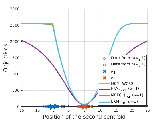
(a)

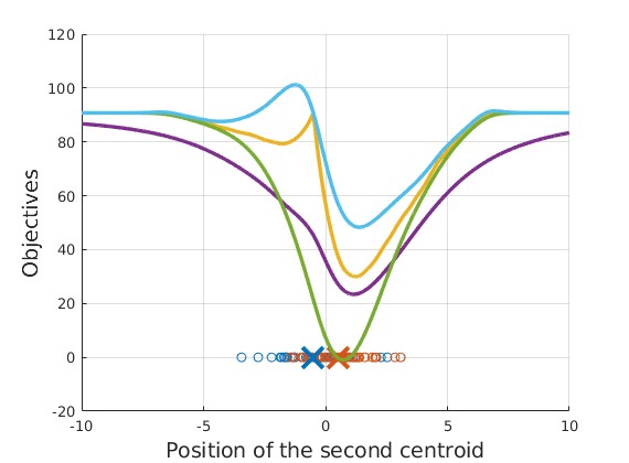
(b)

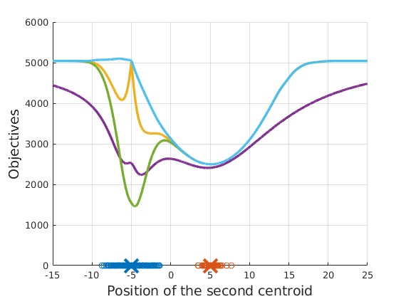
(c)

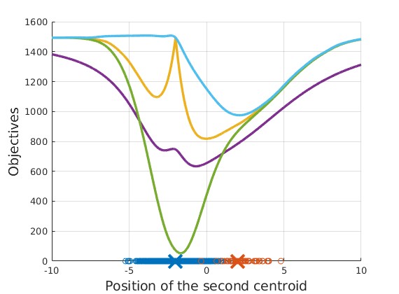
(d)

Figure 2: Objectives of four KM algorithms as a function of the first centroid fixed at $\mu_{1}$ and the second centroid moving along the $x$-axis. The yellow, purple, green, and blue curves are the objective functions of HKM, FKM, MEFC, and EKM, respectively. (a), (b), (c), and (d) present objective functions for different data distributions.

IV-B The Analysis of EKM’s Effectiveness on Imbalanced Data

We demonstrate the effectiveness of EKM by analyzing the gradient of its objective. The gradient of the smoothed WCSS with respect to the distance between data points and centroids can be interpreted as the force exerted by a spring. Positive gradient values represent attractive forces, while negative values represent repulsive forces. The gradient is also associated with membership, where the membership (7) of FKM is equivalent to a power exponent ($1/m$) of $\partial J_{\text{PN}}/\partial d_{kn}$, and the membership (10) of MEFC is equivalent to $\partial J_{\text{LSE}}/\partial d_{kn}$.

A simple example is given to plot the gradient values of different smoothed objectives. We fix two centroids at $-1$ and $+1$, respectively, and move a data point along the $x$-axis. In Fig. 3a we display the gradients of WCSS, $J_{\text{LSE}}$, $J_{\text{PN}}$, and $J_{\text{B}}$ with respect to the distance between the data point and the second centroid. As evident from the figure, data points on the side of the first centroid do not impact the second centroid of HKM, but they do attract the second centroids of FKM and MEFC. This finding supports the previous result in [31] that FKM has a stronger uniform effect than HKM. However, for EKM, data points near the first centroid have repulsive forces on the second centroid, which compensates for the attraction of points on the side of the first centroid to the second centroid, effectively reducing the uniform effect. Furthermore, it is worth noting that for EKM, data points near the second centroid have the strongest attraction forces. Thus, the second centroid is anchored by these data points, making its position less susceptible to noise or outliers. This is the advantage of EKM over imbalanced data clustering algorithms that assign weights to data points based on cluster size.

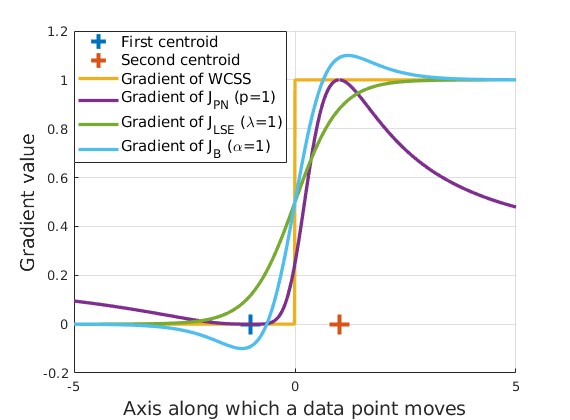
(a)

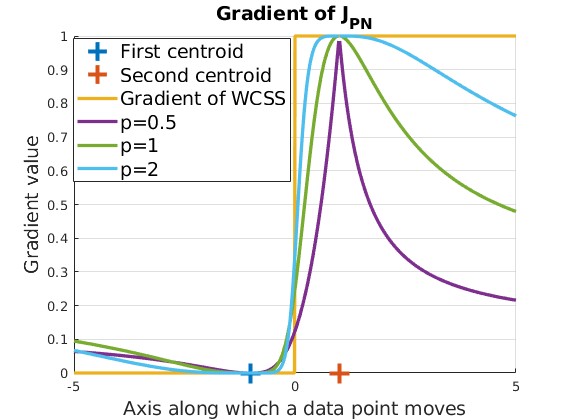
(b)

(c)

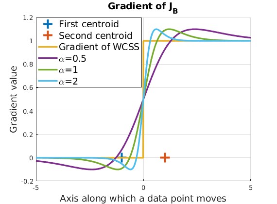
(d)

Figure 3: Gradients of four KM algorithms as a function of a data point moving along the $x$-axis. (a) Gradients of HKM, FKM, MEFC, and EKM with fixed smoothness parameters. (b) Gradients of FKM. (c) Gradients of MEFC. (d) Gradients of EKM.

IV-C The Choice of $\alpha$

The smoothing parameter $\alpha$ has an impact on the clustering result in EKM, but the optimal choice remains unknown, which is not a difficulty unique to EKM. The FKM algorithm also struggles with selecting the optimal fuzzifier value, $m$. Despite numerous studies discussing the selection of $m$, a widely accepted solution has yet to be found [32].

Determining optimal parameters for a clustering algorithm often involves trial and error, as the real data structure is unknown. As a rule of thumb, when the data space dimension is less than or equal to three, setting $\alpha=1$ appears effective after normalizing the data to have a zero mean and unit variance for each dimension. As the data space dimension increases, the data-centroid distance $d_{kn}$ tends to grow, necessitating a decrease in $\alpha$ to ensure that the exponential term $e^{-\alpha d_{kn}}$ remains within a normal range. In this case, we suggest setting $\alpha$ to ten times the data variance and gradually reducing it. A proper $\alpha$ value indicates the presence of repulsive forces, resulting in a sudden increase in centroid distances. Ultimately, techniques for visualizing clustering results can be employed to fine-tune the $\alpha$ value. This strategy is proven effective by experimental examples of deep clustering on the MNIST dataset in Section VI. We further discuss and validate the choice of $\alpha$ in the supplemental material.

V Numerical Experiments

Numerical experiments are conducted to compare the performance of our proposed EKM algorithm with six other algorithms: (1) HKM, (2) FKM, (3) MEFC, (4) csiFKM [19], (5) siibFKM [20], and (6) the Gaussian mixture model. Multiprototype clustering algorithms are not used as benchmarks, as the multiprototype mechanisms can be combined with EKM for fair comparison. This is beyond the scope of this paper because the paper does not intend to find the best KM algorithm to pair with the multiprototype mechanism.

To avoid local optima convergence, each clustering algorithm is executed ten times, presenting the lowest objective value result. Centroids are initialized independently for each replication using the K-means++ algorithm [33]. Convergence is deemed achieved when the relative moving distance of centroids between successive iterations is less than $1\mathrm{e}{-3}$, i.e.,

$$\frac{\bigg{(}\sum_{k=1}^{K}\|\mathbf{c}_{k}^{(\tau)}-\mathbf{c}_{k}^{(\tau-1)}\|_{2}^{2}\bigg{)}^{1/2}}{\bigg{(}\sum_{k=1}^{K}\|\mathbf{c}_{k}^{(\tau)}\|_{2}^{2}\bigg{)}^{1/2}}\leq 1\mathrm{e}{-3}.$$ (44)

The maximum number of iterations is set to 100. FKM, csiFKM, and siibFKM employ a typical fuzzifier value of $m=2$ [34]. The fuzzifier value of MEFC is set to $\lambda=1$ and the smoothness value of EKM is set to $\alpha=1$. We test the algorithms on 12 datasets, including two synthetic and ten real datasets. Because of space limitations, only partial experiment results from six datasets are shown in the paper. Full experiment results with quantitative metrics can be found in the supplemental material. The six datasets are introduced below.

V-A Datasets

V-A1 Synthetic 2-D Ball

We create a synthetic dataset with data independently generated from three distinct normal distributions, each having different means: $(-2,2)$, $(2,-2)$, and $(4,4)$. Their covariance matrices are all identity matrices. The dataset consists of 2,000 samples from the normal distribution with means $(-2,2)$, and 50 samples from the other two normal distributions, resulting in a total of 2,100 samples. The clustering results are shown in Fig. 4.

V-A2 Synthetic 2-D Noisy Ball

We add 100 uniformly distributed noise data samples (around 5% of the number of clean samples) to the synthetic 2-D ball dataset to test the algorithms’ robustness against noise. The clustering outcomes are displayed in Fig. 5.

V-A3 Fisher’s Iris Data

The Fisher’s Iris dataset [35, 36] is a well-known dataset for evaluating the performance of clustering algorithms. It comprises 50 samples from each of three iris species (Iris setosa, Iris virginica, and Iris versicolor). Two features, the width and the length of the sepals, are utilized as clustering features and normalized to have zero means and unit variance. Fig. 6 depicts the clustering results.

V-A4 Imbalanced Fisher’s Iris Data

Because the instance distribution in the Iris dataset is balanced. To examine the algorithms’ capability for imbalanced clustering, we generate an imbalanced Fisher’s Iris data by removing the first 30 instances of Iris setosa, and merging the other two species (Iris virginica and Iris versicolor) into a single class. The clustering results for this dataset are presented in Fig. 7.

V-A5 Wisconsin Diagnostic Breast Cancer

Wisconsin Diagnostic Breast Cancer (WDBC) [37] comprises 30 features of cell nuclei from diagnostic benign and malignant breast tumors, obtained from digitized images of fine-needle aspiration of breast masses. This database contains 569 instances, with a fairly even distribution of 357 benign and 212 malignant cases. We utilize the first three features (mean radius, mean texture, and mean perimeter) for clustering, each normalized with zero mean and unit variance. Fig. 9 presents the clustering results where the mean radius and the mean texture are used as coordinates for visualization.

V-A6 Imbalanced Wisconsin Diagnostic Breast Cancer

The data distribution in WDBC is quite balanced. To evaluate the imbalanced data clustering performance, we remove the first 200 malignant instances in WDBC, resulting in an imbalanced WDBC database with a class distribution of 357 benign and 12 malignant instances. We still use the first three features for clustering, each normalized with zero mean and unit variance. The clustering results are shown in Fig. 9.

V-A7 ColoredChips

This is not a dataset but an image named coloredChips.png from Matlab’s image gallery (shown in Fig. 10a). The purpose of this experiment is to test the algorithms’ performance on the task of color-based image segmentation. The number of clusters is set to five to expect the segmentation of the four colored chips and the background (i.e., the desk surface). Clustering is conducted in the RGB space and the segmentation results can be viewed in Fig. 10b - 10e.

V-B Discussion of Results

In general, these results demonstrate that the proposed EKM algorithm performs competitively on balanced data and outperforms the other clustering algorithms on imbalanced data. In particular, HKM, FKM, and MEFC cannot find the correct clusters in imbalanced datasets. The csiFKM and siibFKM algorithms are sensitive to noise data. Fig. 5c and Fig. 5d show that their centroids are highly deviated from the correct positions because of noise. In comparison, EKM is more robust, as seen in Fig. 5e.

Fig. 9 displays the clustering results of HKM, FKM, GMM, and EKM for the imbalanced WDBC dataset. The strong performance of EKM indicates its potential application in anomaly detection, particularly in identifying clustered anomalies. Although HKM and FKM are also used for anomaly detection, they typically detect isolated anomalies, not clustered ones [38, 39, 40, 41].

The color-based image segmentation results are shown in Fig. 10b - 10e. It can be seen that HKM, FKM, and MEFC divide the background (the desk surface) into two clusters. This happens because the background comprises most pixels, and splitting it into two clusters better balances the number of pixels within the clusters. On the other hand, EKM produces the expected segmentation result.

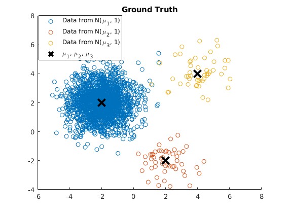
(a)

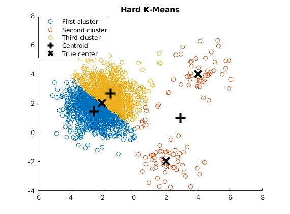
(b)

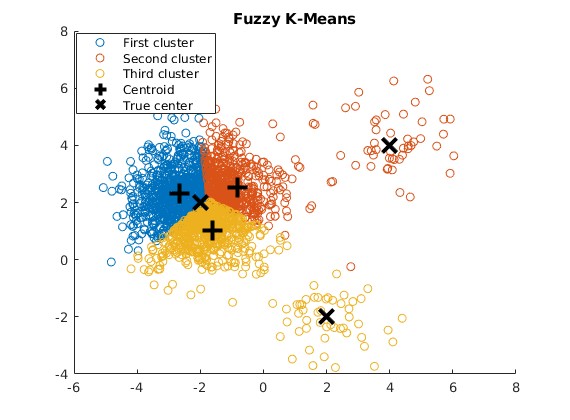
(c)

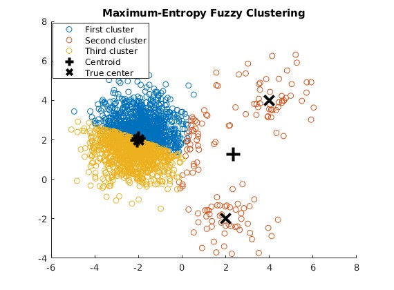
(d)

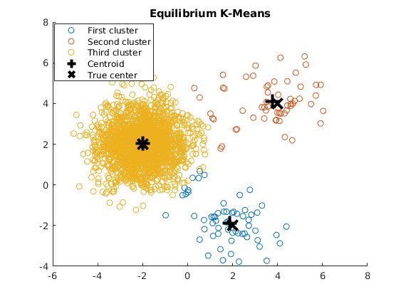
(e)

Figure 4: (a) Synthetic 2-D ball data. (b) Clustering by HKM. (c) Clustering by FKM. (d) Clustering by MEFC. (e) Clustering by EKM.

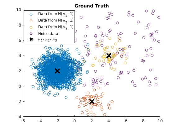
(a)

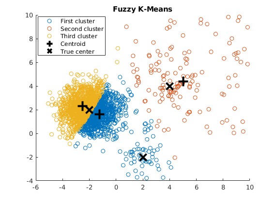
(b)

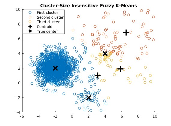
(c)

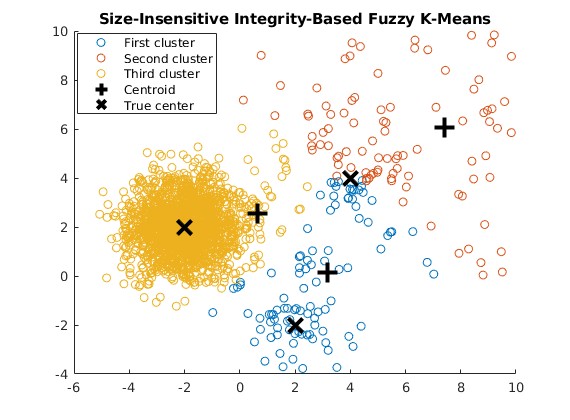
(d)

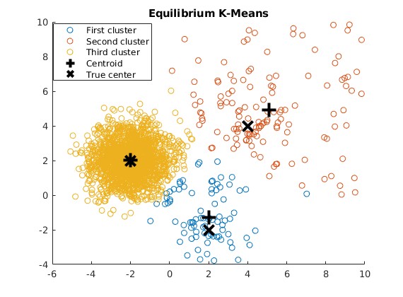
(e)

Figure 5: (a) Synthetic 2-D noisy ball data. (b) Clustering by FKM. (c) Clustering by csiFKM. (d) Clustering by siibFKM. (e) Clustering by EKM.

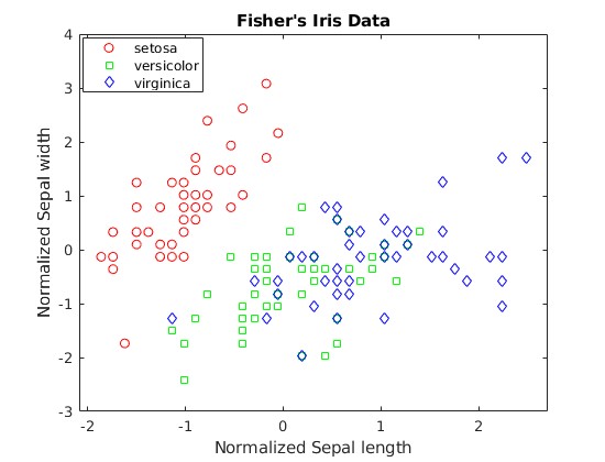
(a)

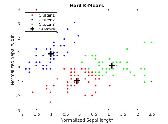
(b)

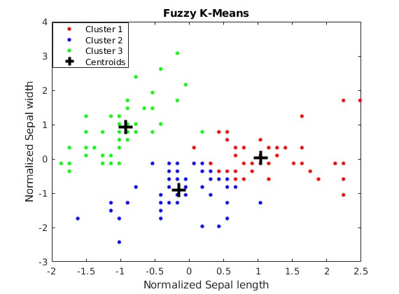
(c)

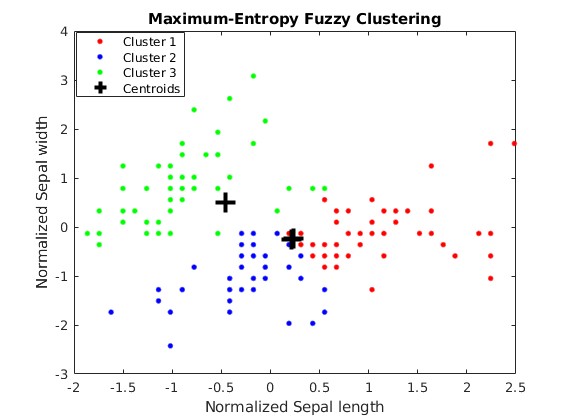
(d)

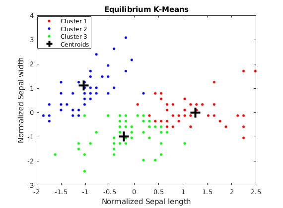
(e)

Figure 6: (a) Fisher’s Iris data. (b) Clustering by HKM. (c) Clustering by FKM. (d) Clustering by MEFC. (e) Clustering by EKM.

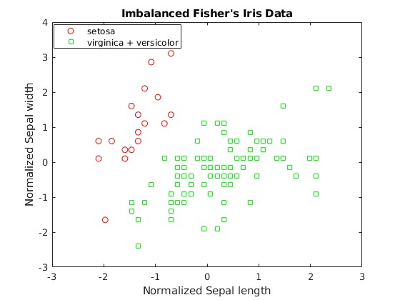
(a)

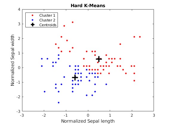
(b)

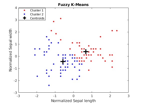
(c)

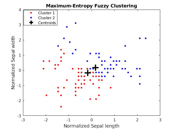
(d)

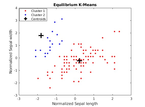
(e)

Figure 7: (a) Imbalanced Fisher’s Iris data. (b) Clustering by HKM. (c) Clustering by FKM. (d) Clustering by MEFC. (e) Clustering by EKM.

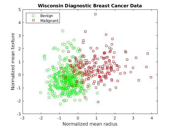
(a)

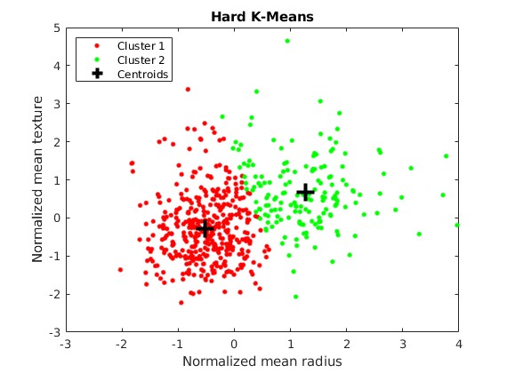
(b)

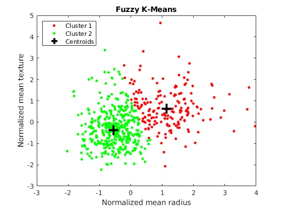
(c)

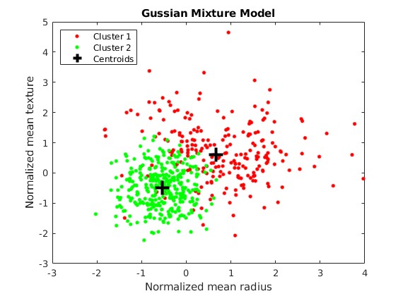
(d)

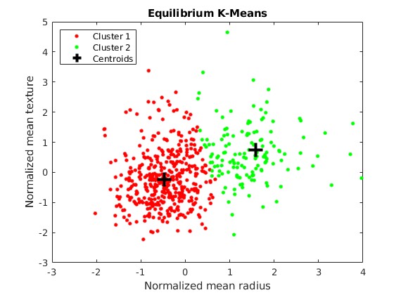
(e)

Figure 8: (a) Wisconsin Diagnostic Breast Cancer dataset. Three features are used for clustering and two of them are used for visualization. (b) Clustering by HKM. (c) Clustering by FKM. (d) Clustering by GMM. (e) Clustering by EKM.

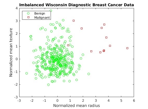
(a)

(b)

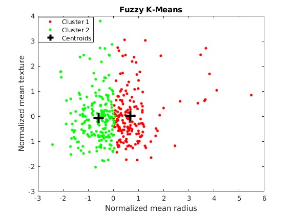
(c)

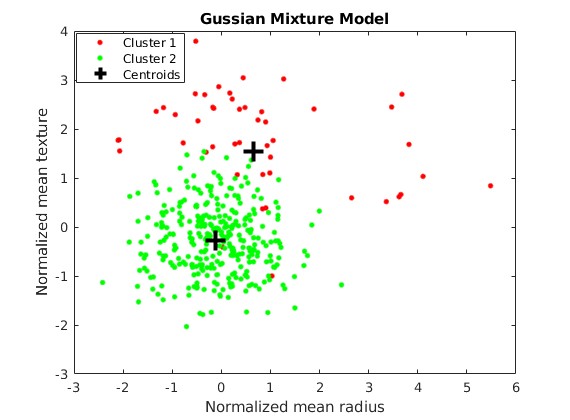
(d)

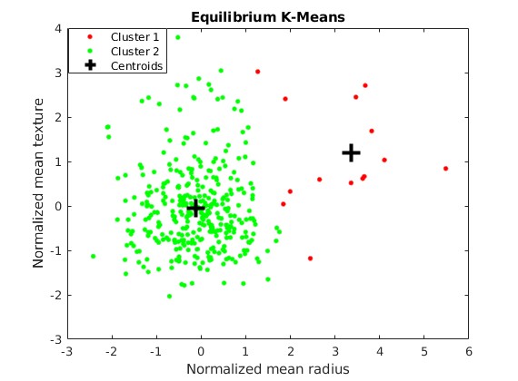
(e)

Figure 9: (a) Imbalanced Wisconsin Diagnostic Breast Cancer dataset. (b) Clustering by HKM. (c) Clustering by FKM. (d) Clustering by GMM. (e) Clustering by EKM.

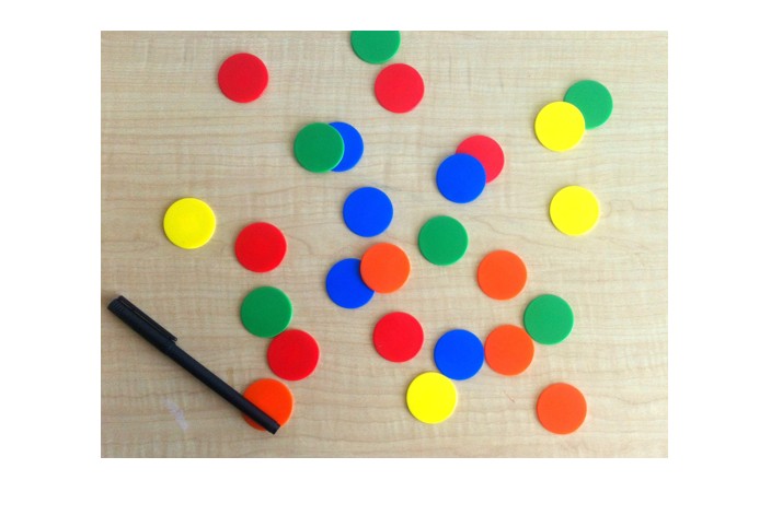
(a)

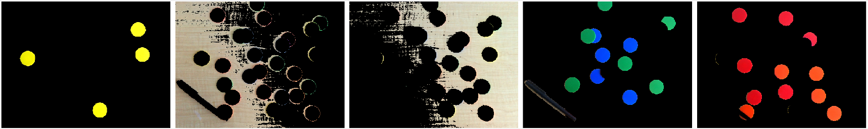
(b)

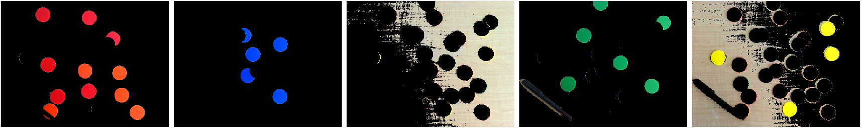
(c)

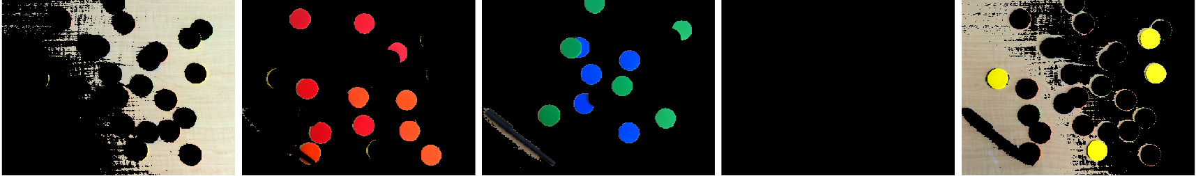
(d)

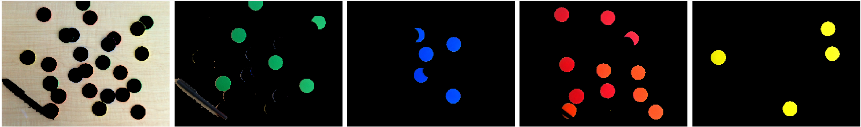
(e)

Figure 10: (a) coloredChips.png (b) Segmentation by HKM. (c) Segmentation by FKM. (d) Segmentation by MEFC. (e) Segmentation by EKM.

VI Deep Clustering

Clustering algorithms using Euclidean distance for defining similarity often face challenges when clustering high-dimensional data, such as images, due to the small distance differences between various point pairs in high-dimensional space [42]. Deep clustering is a technique that addresses this issue by employing DNNs to map high-dimensional data non-linearly to low-dimensional representation, making the subsequent clustering easier. Most existing deep clustering approaches combine DNNs with HKM, e.g., [12, 13, 14]. However, this design is less favorable to imbalanced datasets [13]. In this section, we provide an example of replacing HKM with EKM in a popular deep clustering framework, showing its performance improvement on an imbalanced dataset derived from the MNIST.

VI-A Optimization Procedure

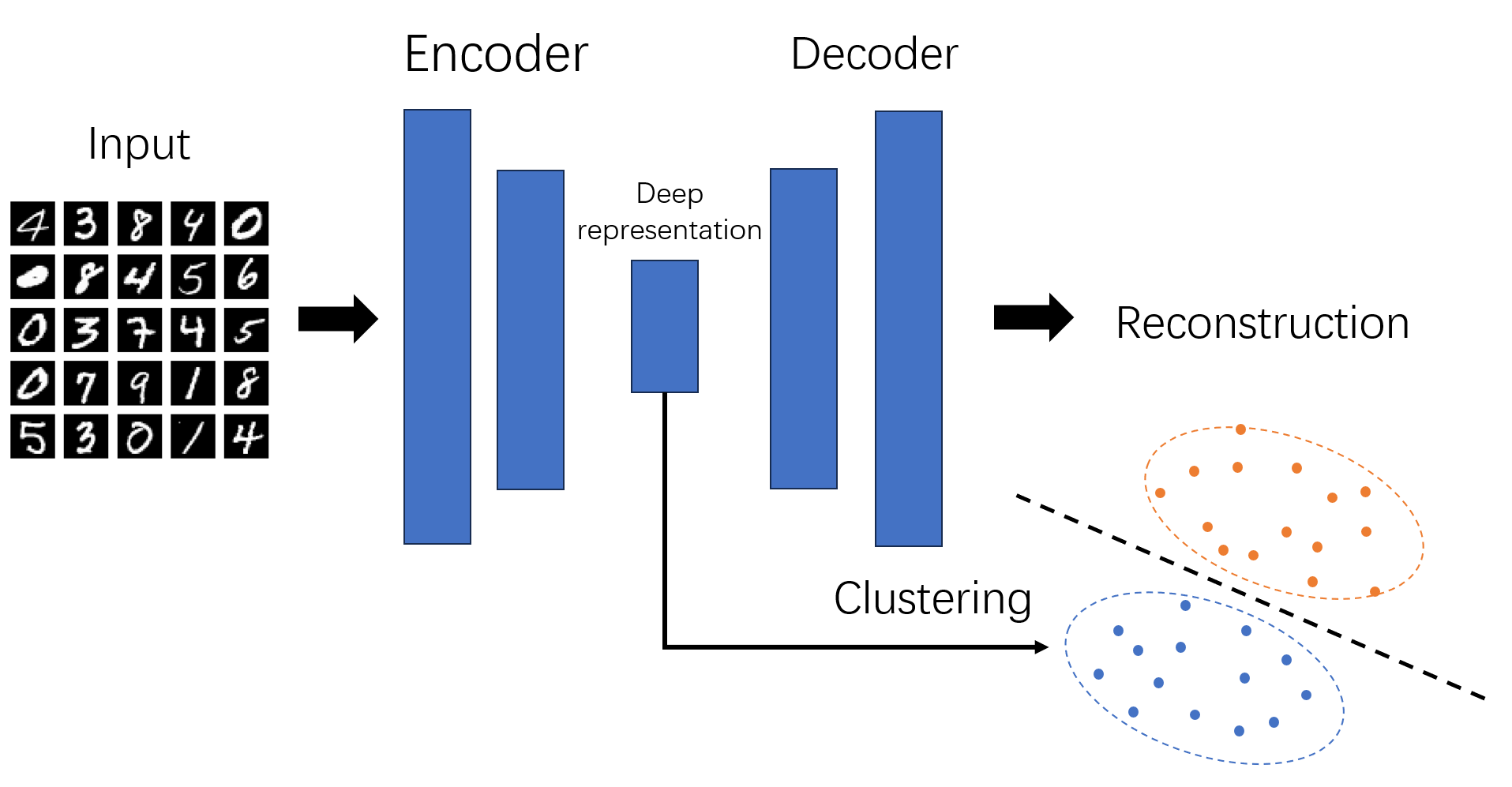
Figure 11: Illustration of the DCN framework [12]. The parameters of the encoder, decoder, and clustering model are optimized jointly to minimize the reconstruction error and clustering error.

Deep clustering network (DCN) [12] is a popular deep clustering framework, as illustrated in Fig. 11. Essentially, DCN maps high-dimensional data to a low-dimensional representation through an autoencoder network. An autodecoder follows the autoencoder, mapping the representation back to the original high-dimension space (i.e., reconstruction). To ensure that the low-dimensional representation maintains the primary information of the original data, the autoencoder and autodecoder are jointly trained to minimize the reconstruction error. Additionally, to create a clustering-friendly structure in the low-dimensional representation, a clustering error is minimized along with the reconstruction error. DCN uses an alternating optimization algorithm to minimize the total error, and the optimization process is described below.

First, the autoencoder and the autodecoder are jointly trained to reduce the following loss for the incoming data $\mathbf{x}_{n}$:

$$\min_{\bm{\theta}_{e},\bm{\theta}_{d}}L^{n}=l(\bm{g}(\bm{f}(\mathbf{x}_{n})),\mathbf{x}_{n})+\beta\|\bm{f}(\mathbf{x}_{n})-\mathbf{C}\mathbf{s}_{n}\|_{2}^{2},$$ (45)

where $\bm{f}(\cdot)$ and $\bm{g}(\cdot)$ are simplified symbols for autoencoder $\bm{f}(\cdot;\,\bm{\theta}_{e})$ and autodecoder $\bm{g}(\cdot;\,\bm{\theta}_{d})$, respectively. The function $l(\cdot)$ is the least-squares loss $l(\hat{\mathbf{x}},\mathbf{x})=\|\hat{\mathbf{x}}-\mathbf{x}\|_{2}^{2}$ to measure the reconstruction error. The assignment vector $\mathbf{s}_{n}\in\mathbb{R}^{K\times 1}$ has only one non-zero element and $\mathbf{1}^{\mathsf{T}}\mathbf{s}_{n}=1$, indicating which cluster the $n$-th data belongs to, and the $k$-th column of $\mathbf{C}=[\mathbf{c}_{1},\cdots,\mathbf{c}_{K}]$ is the centroid of the $k$-th cluster. The parameter $\beta$ balances the reconstruction error versus the clustering error. Then, the network parameters $\{\bm{\theta}_{e},\bm{\theta}_{d}\}$ are fixed, and the parameters $\{\mathbf{s}_{n}\}$ are updated as follows:

$$s_{j,n}\leftarrow\begin{cases}1,&\text{if}\,j=\operatorname*{arg\,min}_{k=\{1,\cdots,K\}}\|\bm{f}(\mathbf{x}_{n})-\mathbf{c}_{k}\|_{2},\\ 0,&\text{otherwise,}\end{cases}$$ (46)

where $s_{j,n}$ is the $j$-th element of $\mathbf{s}_{n}$. Finally, $\mathbf{C}$ is updated by the batch-learning version of the HKM algorithm:

$$\mathbf{c}_{k}\leftarrow\mathbf{c}_{k}+(1/m_{k}^{n})(\bm{f}(\mathbf{x}_{n})-\mathbf{c}_{k})s_{k,n},$$ (47)

where $m_{k}^{n}$ is the number of samples assigned to the $k$-th cluster before the incoming data $\mathbf{x}_{n}$, controlling the learning rate of the $k$-th centroid. Overall, the optimization procedure of DCN with HKM alternates between updating networks parameters $\{\bm{\theta}_{e},\bm{\theta}_{d}\}$ by solving (45) and updating HKM parameters $\{\mathbf{C},\{\mathbf{s}_{n}\}\}$ by (46) and (47).

However, the centroid updating rule (47) is problematic for imbalanced data due to the uniform effect. To address this issue, we propose to replace (47) with the batch-learning version of EKM:

$$\mathbf{c}_{k} \leftarrow\mathbf{c}_{k}-(1/m_{k}^{n})\partial_{\mathbf{c}_{k}}J_{B}(\mathbf{c}_{1},\cdots,\mathbf{c}_{K})$$ (48)

$$=\mathbf{c}_{k}+(1/m_{k}^{n})\frac{e^{-\alpha d_{kn}}}{\sum_{i=1}^{K}e^{-\alpha d_{in}}}\big{[}1-\alpha(d_{kn}$$

$$-\frac{\sum_{i=1}^{K}d_{in}e^{-\alpha d_{in}}}{\sum_{i=1}^{K}e^{-\alpha d_{in}}})\big{]}(\bm{f}(\mathbf{x}_{n})-\mathbf{c}_{k}),$$

where $d_{kn}=\frac{1}{2}\|\bm{f}(\mathbf{x}_{n})-\mathbf{c}_{k}\|_{2}^{2}$. There are other details and tricks to implement DCN, such as the initialization of the networks. We only introduce the part related to our contribution, and for the rest, the readers can refer to the original paper of DCN [12].

VI-B Clustering Performance on MNIST

To implement DCN, we refer to the code provided by one of its authors, available at https://github.com/boyangumn/DCN-New. We use the default neural network structure and hyperparameters. In particular, the deep representation dimension is set to ten, and the parameter $\beta$ is set to one. The smoothness parameter $\alpha$ for EKM is determined by the strategy introduced in Section IV-C. We evaluate clustering performance using three widely accepted metrics: including normalized mutual information (NMI), adjusted Rand index (ARI), and clustering accuracy (ACC). NMI and ACC range from 0 to 1, with zero representing the worst and one representing the best. ARI ranges from -1 to 1, with minus one representing the worst and one representing the best.

We first validate the algorithms on the full MNIST dataset [43], containing 70,000 gray images of handwritten digits from 0 to 9. We set the smoothness parameter of EKM to $\alpha=5\mathrm{e}-3$. The clustering results are presented in TABLE I, where we compare the proposed DCN+EKM with DCN+HKM and stacked autoencoder (SAE). SAE is a specific version of DCN that only minimizes the reconstruction error. We omit the results of DCN+FKM and DCN+MEFC due to space limitations and their poorer performance compared to DCN+HKM. The results show that DCN outperforms SAE, highlighting the importance of a clustering-friendly representation. The table also reveals that DCN+EKM performs similarly to DCN+HKM for this balanced dataset.

To evaluate the performance of the algorithms for imbalanced data clustering, we remove the MNIST dataset’s training set samples with numbers 1 to 9 (leaving only the test set samples). This imbalanced dataset has 15,923 images, with around 6,900 being the number 0 and the remaining numbers (1 to 9) being around 1,000. We set the smoothness parameter of EKM to $\alpha=3.8\mathrm{e}-3$. The clustering results are summarised in TABLE II, showing that DCN+EKM significantly outperforms DCN+HKM. To analyze the reason, we use t-SNE [44] to map the ten-dimensional representation obtained by DCN to a two-dimensional space for visualization, with the results displayed in Fig. 12. We observe that the deep representation obtained by DCN+EKM is more discriminative than DCN+HKM, and DCN+EKM successfully separates the large class (number 0) from other small classes, while DCN+HKM erroneously groups the large class into four clusters.

TABLE I: Evaluation on full MNIST

Methods SAE+HKM DCN+HKM SAE+EKM DCN+EKM NMI 0.725 0.798 0.711 0.813 ARI 0.667 0.744 0.642 0.731 ACC 0.795 0.837 0.782 0.808

TABLE II: Evaluation on imbalanced MNIST

Methods SAE+HKM DCN+HKM SAE+EKM DCN+EKM NMI 0.551 0.584 0.583 0.701 ARI 0.317 0.325 0.396 0.826 ACC 0.413 0.434 0.497 0.784

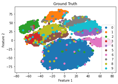
(a)

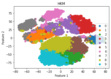
(b)

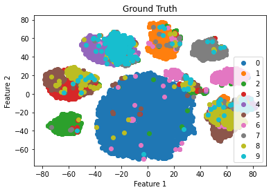
(c)

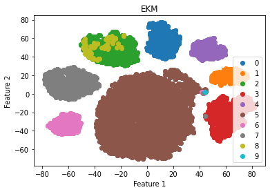
(d)

Figure 12: Visualization of low-dimensional DCN representations by t-SNE. (a) Representations obtained by DCN+HKM, colored by true labels. (b) Representations obtained by DCN+HKM, colored by clusters of HKM. (c) Representations obtained by DCN+EKM, colored by true labels. (d) Representations obtained by DCN+EKM, colored by clusters of EKM.

VII Conclusion

This paper presents equilibrium K-means (EKM), a novel clustering algorithm that is effective for imbalanced data. EKM is simple, interpretable, scalable to large datasets, and capable of finding unequal-sized clusters, making it a better alternative for hard K-means (HKM) and fuzzy K-means (FKM) for imbalanced data. Experimental results on real datasets from various domains demonstrate that EKM outperforms HKM and FKM on datasets with imbalanced data and performs comparably on datasets with balanced data. Furthermore, we provide a general framework that unifies HKM, FKM, and EKM. We encourage readers to explore and develop new K-means algorithms based on this more flexible framework to address other specific K-clustering problems besides imbalanced data distribution.

Appendix A Proof of Theorem 1

For concise and tidy, we denote the partial derivative $\frac{\partial h}{\partial d_{k}}(d_{1n}^{(\tau)},\cdots,d_{Kn}^{(\tau)})$ as $\frac{\partial h}{\partial d_{k}}|_{n,{\tau}}$. Since $h$ is a concave function at $[0,\,+\infty)^{K}$, we have

$$h(d_{1n},\cdots,d_{Kn})$$ (49)

$$\leq h(d_{1n}^{(\tau)},\cdots,d_{Kn}^{(\tau)})+\sum_{k=1}^{K}\frac{\partial h}{\partial d_{k}}\bigg{|}_{n,{\tau}}\cdot(d_{kn}-d_{kn}^{(\tau)}),$$

which holds for any $n\in\{1,\cdots,N\}$ and $d_{1n},\cdots,d_{Kn}\in[0,\,+\infty)$. Summing over $n$, it follows that

$$J(\mathbf{c}_{1},\cdots,\mathbf{c}_{K})\\ \leq\sum_{n=1}^{N}\bigg{[}h(d_{1n}^{(\tau)},\cdots,d_{Kn}^{(\tau)})+\sum_{k=1}^{K}\frac{\partial h}{\partial d_{k}}\bigg{|}_{n,{\tau}}\cdot(d_{kn}-d_{kn}^{(\tau)})\bigg{]}\\ =J(\mathbf{c}_{1}^{(\tau)},\cdots,\mathbf{c}_{K}^{(\tau)})+\frac{1}{2}\sum_{k=1}^{K}\sum_{n=1}^{N}\bigg{(}\frac{\partial h}{\partial d_{k}}\bigg{|}_{n,{\tau}}\cdot\big{(}\|\mathbf{x}_{n}-\mathbf{c}_{k}\|_{2}^{2}\\ -\|\mathbf{x}_{n}-\mathbf{c}_{k}^{(\tau)}\|_{2}^{2}\big{)}\bigg{)}.$$ (50)

Denote the function on the right side of the inequality as $M(\mathbf{c}_{1},\cdots,\mathbf{c}_{K})$. With the boundness condition, we have $\sum_{n=1}^{N}\frac{\partial h}{\partial d_{k}}\big{|}_{n,\tau}>0$ for any $k$ and $\tau$, thus, $M$ is a quadratic function and strictly convex, with the unique global minimizer at $(\mathbf{c}_{1}^{(\tau+1)},\cdots,\mathbf{c}_{K}^{(\tau+1)})$ defined by (42). Denote $J(\mathbf{c}_{1}^{(\tau)},\cdots,\mathbf{c}_{K}^{(\tau)})$ as $J^{(\tau)}$, $M(\mathbf{c}_{1}^{(\tau)},\cdots,\mathbf{c}_{K}^{(\tau)})$ as $M^{(\tau)}$, and $\partial_{\mathbf{c}_{k}}J(\mathbf{c}_{1}^{(\tau)},\cdots,\mathbf{c}_{K}^{(\tau)})$ as $\partial_{\mathbf{c}_{k}}J^{(\tau)}$. Each iteration of the centroid will reduce the objective function by

$$J^{(\tau)}-J^{(\tau+1)}$$ (51)

$$\geq J^{(\tau)}-M^{(\tau+1)}$$

$$=\frac{1}{2}\sum_{k=1}^{K}\sum_{n=1}^{N}\frac{\partial h}{\partial d_{k}}\bigg{|}_{n,\tau}\cdot\big{(}\|\mathbf{x}_{n}-\mathbf{c}_{k}^{(\tau)}\|_{2}^{2}-\|\mathbf{x}_{n}-\mathbf{c}_{k}^{(\tau+1)}\|_{2}^{2}\big{)}$$

substituting (42)

$$=\frac{1}{2}\sum_{k=1}^{K}\sum_{n=1}^{N}\frac{\partial h}{\partial d_{k}}\bigg{|}_{n,\tau}\cdot\big{(}\|\mathbf{x}_{n}-\mathbf{c}_{k}^{(\tau)}\|_{2}^{2}-\|\mathbf{x}_{n}-\mathbf{c}_{k}^{(\tau)}$$

$$+\gamma_{k}^{(\tau)}\partial_{\mathbf{c}_{k}}J^{(\tau)}\|_{2}^{2}\big{)}$$

$$=\frac{1}{2}\sum_{k=1}^{K}\sum_{n=1}^{N}\frac{\partial h}{\partial d_{k}}\bigg{|}_{n,\tau}\cdot\big{(}-(\gamma_{k}^{(\tau)})^{2}\|\partial_{\mathbf{c}_{k}}J^{(\tau)}\|_{2}^{2}$$

$$-2\gamma_{k}^{(\tau)}(\mathbf{x}_{n}-\mathbf{c}_{k}^{(\tau)})^{\mathsf{T}}\partial_{\mathbf{c}_{k}}J^{(\tau)}\big{)}$$

using $$\gamma_{k}^{(\tau)}=\frac{1}{\sum_{n=1}^{N}\frac{\partial h}{\partial d_{k}}|_{n,\tau}}$$

and $$\partial_{\mathbf{c}_{k}}J^{(\tau)}=-\sum_{n=1}^{N}\frac{\partial h}{\partial d_{k}}\cdot(\mathbf{x}_{n}-\mathbf{c}_{k}^{(\tau)})$$

$$=\sum_{k=1}^{K}-\frac{1}{2}\gamma^{(\tau)}_{k}\|\partial_{\mathbf{c}_{k}}J^{(\tau)}\|_{2}^{2}+\sum_{k=1}^{K}\gamma_{k}^{(\tau)}\|\partial_{\mathbf{c}_{k}}J^{(\tau)}\|_{2}^{2}$$

$$=\sum_{k=1}^{K}\frac{1}{2}\gamma_{k}^{(\tau)}\|\partial_{\mathbf{c}_{k}}J^{(\tau)}\|_{2}^{2}$$

with the boundness condition of $$\gamma_{k}^{(\tau)}$$

$$\geq\frac{1}{2}\epsilon\sum_{k=1}^{K}\|\partial_{\mathbf{c}_{k}}J^{(\tau)}\|_{2}^{2},$$

where $\epsilon$ is a positive number. Hence, the sequence $(J^{(1)},J^{(2)},\cdots)$ is non-increasing, and with the boundness condition that $h>-\infty$, we have $\lim_{\tau\to+\infty}(J^{(\tau)}-J^{(\tau+1)})\to 0$. If the left side of the inequality (LABEL:theorem1_proof_inequality) converges to zero, the right side of the inequality also converges to zero since it is non-negative. Consequently, we have $\lim_{\tau\to+\infty}\partial_{\mathbf{c}_{k}}J^{(\tau)}\to 0$ for all $k$. Therefore, the sequence $(\mathbf{c}_{k}^{(\tau)})$ converges to a stationary point of the objective function $J$. Because $(J^{(1)},J^{(2)},\cdots)$ is non-increasing, only (local) minimizers or saddle points appear as limit points.

Supplemental Materials: Imbalanced Data Clustering using Equilibrium K-Means

supplement

We evaluate the clustering performance of the proposed Equilibrium K-means (EKM) on ten real datasets. Four datasets (Iris, Imbalanced Iris, Wisconsin Diagnostic Breast Cancer (WDBC), and Imbalanced WDBC) are discussed in detail in the main text. This supplemental material presents the results for the remaining six datasets from the UCI repository (available at https://archive.ics.uci.edu/datasets): Wine, Ecoli, Image Segmentation (IS), Htru2, Rice, and Dry Bean. A detailed description of all ten datasets can be found in TABLE SI, ordered according to the imbalance level measured by CV0, which we will define later. Datasets with a lower order have higher CV0 values, indicating a higher imbalance level. We provide some necessary explanations for this table below.

In the “Feature” column, the format “x (y)” indicates that the dataset has y features, with x features used for clustering. For instance, the Iris dataset has four features, with two used for clustering. Only the four datasets in the main text use partial features for clustering, which serves the purpose of visualizing clustering results. For the additional six datasets, all features are used since visualization is not required. In the “CV0” column, we calculate the coefficient of variation (CV) to measure data imbalance. CV is defined as the ratio of the standard deviation to the mean. CV is defined as the ratio of the standard deviation to the mean. Mathematically, given the number of instances in each class as $N_{1},\cdots,N_{K}$, we have

$$\text{CV}=\text{std}(\mathbf{N})/\text{mean}(\mathbf{N}),$$

where

$$\text{mean}(\mathbf{N})=\frac{\sum_{k=1}^{K}N_{k}}{K},$$

and

$$\text{std}(\mathbf{N})=\sqrt{\frac{\sum_{k=1}^{K}(N_{k}-\text{mean}(\mathbf{N}))^{2}}{K-1}}.$$

In general, the larger the CV value, the greater the imbalance of the data.

Each dataset is normalized so that each feature has zero mean and unit variance. The number of clusters is assumed to be equal to the number of classes for all datasets. For the supplementary six datasets, the smoothness parameter $\alpha$ is chosen as follows:

$$\alpha=2/\bar{d}_{0n},$$

where $\bar{d}_{0n}=\frac{1}{2}\sum_{n=1}^{N}\|\mathbf{x}_{n}\|_{2}^{2}/N$, $\mathbf{x}_{n}$ is the $n$-th data point, and $N$ is the total number of data points. The value $\bar{d}_{0n}$ can be interpreted as a data variance after the normalization of zero data mean. The normalized mutual information (NMI), adjusted Rand index (ARI), and clustering accuracy (ACC) metrics of each algorithm on the ten datasets are presented in TABLE SII. Bold values indicate the best results. We also include three more metrics: “CV1”, ”DCV” and ”Running time” for readers’ interest. “CV1” is the CV value of the clustering result. “DCV” is the difference between CV0 and CV1, i.e., $\text{DCV}=\text{CV}0-\text{CV}1$. A positive DCV value indicates that the data distribution in the true classes is more imbalanced than in the clusters, while a negative DCV value means the data distribution in the true classes is more uniform than in the clusters. “Running time” is the sum of the running time of ten replicates.

We observe that the proposed EKM generally outperforms the other six algorithms on the last four datasets with CV values greater than 0.5. EKM outperforms other algorithms on two of the top six datasets with CV values less than 0.5. On the rest of the datasets, EKM still has a competitive performance. The running time of EKM is also comparable to FKM. Overall, these results demonstrate that EKM is an efficient algorithm for clustering balanced and imbalanced data.

TABLE SI: Detailed description of REAL-WORLD Datasets

Dataset	Instance	Feature	Class	CV0
Iris	150	2 (4)	3	0
IS	2310	19 (19)	7	0
Wine	178	13 (13)	3	0.1939
Rice	3810	7 (7)	2	0.2042
WDBC	569	3 (30)	3	0.3604
Dry Bean	13611	16 (16)	7	0.4951
Imbalanced Iris	120	2 (4)	2	0.9428
Ecoli	336	7 (7)	8	1.1604
Imbalanced WDBC	369	3 (30)	2	1.3222
Htru2	17898	8 (8)	2	1.4142

TABLE SII: Experimental results of different algorithms on real-world datasets

Dataset	Measurement	HKM	FKM	MEFC	csiFKM	siibFKM	GMM	EKM
Iris	NMI	0.5945	0.5671	0.5194	0.5671	0.5675	0.6775	0.5457
	ARI	0.5462	0.5328	0.5291	0.5328	0.5281	0.5354	0.5134
	ACC	0.7867	0.7800	0.7933	0.7800	0.7800	0.7000	0.7733
	CV1	0.0346	0.0200	0.1217	0.0200	0.1442	0.8902	0.0346
	DCV	-0.0346	-0.0200	-0.1217	-0.0200	-0.1442	-0.8902	-0.0346
	Running time	0.0113	0.0111	0.0305	0.0142	0.1844	0.0715	0.0328
IS	NMI	0.5864	0.5953	0.6222	0.5971	0.5997	0.5657	0.6463
	ARI	0.4605	0.4973	0.4995	0.4962	0.3214	0.4456	0.5161
	ACC	0.5455	0.6455	0.5944	0.6433	0.5861	0.5641	0.5944
	CV1	0.8246	0.2450	0.6433	0.4617	1.0377	0.5037	0.6582
	DCV	-0.8246	-0.2450	-0.6433	-0.4617	-1.0377	-0.5037	-0.6582
	Running time	0.0321	0.4714	0.2616	0.7913	49.5369	1.0463	0.7205
Wine	NMI	0.8759	0.8759	0.8759	0.8610	0.3361	0.8466	0.8920
	ARI	0.8975	0.8975	0.8975	0.8804	0.1355	0.8649	0.9134
	ACC	0.9663	0.9663	0.9663	0.9607	0.5562	0.9551	0.9719
	CV1	0.1242	0.1242	0.1242	0.1219	1.1513	0.1070	0.1403
	DCV	0.0696	0.0696	0.0696	0.0720	-0.9574	0.0868	0.0535
	Running time	0.0075	0.0153	0.0088	0.0126	1.6469	0.0515	0.0094
Rice	NMI	0.5685	0.5688	0.5699	0.5554	0.5415	0.4891	0.5653
	ARI	0.6815	0.6824	0.6833	0.6642	0.6394	0.5649	0.6772
	ACC	0.9129	0.9131	0.9134	0.9076	0.9000	0.8759	0.9115
	CV1	0.2442	0.2183	0.2309	0.2977	0.3623	0.0163	0.2643
	DCV	-0.0401	-0.0141	-0.0267	-0.0935	-0.1581	0.1878	-0.0601
	Running time	0.0200	0.0438	0.0357	0.1032	2.1275	0.2303	0.0397
WBDC	NMI	0.4920	0.4870	0.5005	0.4423	0.2951	0.4618	0.4906
	ARI	0.5844	0.5963	0.6257	0.4402	0.2797	0.5722	0.5340
	ACC	0.8840	0.8875	0.8963	0.8366	0.7750	0.8787	0.8682
	CV1	0.5990	0.5393	0.4051	0.8227	0.9768	0.2461	0.7133
	DCV	-0.2386	-0.1790	-0.0447	-0.4623	-0.6164	0.1143	-0.3529
	Running time	0.0156	0.0226	0.0171	0.0385	1.7632	0.0894	0.0160
Dry Bean	NMI	0.7138	0.7055	0.7050	0.6990	0.6673	0.7429	0.6859
	ARI	0.6687	0.6676	0.6565	0.6607	0.6170	0.6914	0.5792
	ACC	0.7865	0.8373	0.7834	0.8001	0.8032	0.8160	0.7478
	CV1	0.5616	0.4697	0.5441	0.5154	0.5394	0.5480	0.6385
	DCV	-0.0666	0.0254	-0.0491	-0.0203	-0.0444	-0.0529	-0.1434
	Running time	0.2186	1.3271	0.6290	1.8517	139.5876	3.4712	0.8499
Imbalanced Iris	NMI	0.0001	0.0247	0.0061	0.6414	0.6870	0.9101	0.9101
	ARI	-0.0053	0.0049	-0.0023	0.7421	0.7865	0.9582	0.9582
	ACC	0.5250	0.5500	0.5250	0.9500	0.9583	0.9917	0.9917
	CV1	0.1179	0.0471	0.0236	1.0842	1.0607	0.9664	0.9664
	DCV	0.8250	0.8957	0.9192	-0.1414	-0.1179	-0.0236	-0.0236
	Running time	0.0057	0.0121	0.0142	0.0257	0.1474	0.0146	0.0115
Ecoli	NMI	0.6370	0.5837	0.6087	0.5999	0.6026	0.6015	0.6530
	ARI	0.4953	0.4113	0.4704	0.4176	0.4468	0.6149	0.5202
	ACC	0.6310	0.5863	0.6190	0.6012	0.6012	0.6964	0.6458
	CV1	0.6871	0.4671	0.7517	0.4482	0.7770	1.0893	0.7001
	DCV	0.4733	0.6933	0.4087	0.7123	0.3835	0.0711	0.4604
	Running time	0.0255	0.2672	0.0760	0.1770	5.3315	0.1939	0.0886
Imbalanced WBDC	NMI	0.0966	0.0848	0.0828	0.6846	0.3893	0.3038	0.6907
	ARI	0.0337	0.0184	0.0158	0.7855	0.5156	0.3323	0.8308
	ACC	0.6260	0.5827	0.5745	0.9892	0.9539	0.9051	0.9892
	CV1	0.2644	0.1418	0.1188	1.3529	1.2073	1.0540	1.3069
	DCV	1.0578	1.1804	1.2034	-0.0307	0.1150	0.2683	0.0153
	Runing time	0.0141	0.0234	0.0094	0.0959	1.2488	0.0870	0.0535
Htru2	NMI	0.4068	0.4101	0.4076	0.0547	0.3854	0.2611	0.5869
	ARI	0.6071	0.5798	0.6076	0.0217	0.5967	0.3504	0.7331
	ACC	0.9366	0.9253	0.9366	0.9097	0.9428	0.8473	0.9660
	CV1	1.0891	1.0125	1.0882	1.4107	1.1813	0.7805	1.2342
	DCV	0.3251	0.4017	0.3260	0.0035	0.2329	0.6337	0.1800
	Running time	0.0825	0.2913	0.1094	2.0558	68.3254	0.4956	0.1119

References

- [1] B. Krawczyk, “Learning from imbalanced data: open challenges and future directions,” Progress in Artificial Intelligence, vol. 5, no. 4, pp. 221–232, 2016.
- [2] H. He and E. A. Garcia, “Learning from imbalanced data,” IEEE Transactions on knowledge and data engineering, vol. 21, no. 9, pp. 1263–1284, 2009.
- [3] Y. Tang, Y.-Q. Zhang, N. V. Chawla, and S. Krasser, “Svms modeling for highly imbalanced classification,” IEEE Transactions on Systems, Man, and Cybernetics, Part B (Cybernetics), vol. 39, no. 1, pp. 281–288, 2008.
- [4] C. Huang, Y. Li, C. C. Loy, and X. Tang, “Learning deep representation for imbalanced classification,” in Proceedings of the IEEE conference on computer vision and pattern recognition, 2016, pp. 5375–5384.
- [5] Y. Lu, Y.-M. Cheung, and Y. Y. Tang, “Self-adaptive multiprototype-based competitive learning approach: A k-means-type algorithm for imbalanced data clustering,” IEEE transactions on cybernetics, vol. 51, no. 3, pp. 1598–1612, 2019.
- [6] W. Press, S. Teukolsky, W. Vetterling, and B. Flannery, “Gaussian mixture models and k-means clustering,” Numerical recipes: the art of scientific computing, pp. 842–850, 2007.
- [7] E. Shireman, D. Steinley, and M. J. Brusco, “Examining the effect of initialization strategies on the performance of gaussian mixture modeling,” Behavior research methods, vol. 49, pp. 282–293, 2017.
- [8] J. MacQueen et al., “Some methods for classification and analysis of multivariate observations,” in Proceedings of the fifth Berkeley symposium on mathematical statistics and probability, vol. 1, no. 14. Oakland, CA, USA, 1967, pp. 281–297.
- [9] S. Lloyd, “Least squares quantization in pcm,” IEEE transactions on information theory, vol. 28, no. 2, pp. 129–137, 1982.
- [10] J. C. Bezdek, Pattern recognition with fuzzy objective function algorithms. Springer Science & Business Media, 2013.
- [11] A. Coates and A. Y. Ng, “Learning feature representations with k-means,” in Neural Networks: Tricks of the Trade: Second Edition. Springer, 2012, pp. 561–580.
- [12] B. Yang, X. Fu, N. D. Sidiropoulos, and M. Hong, “Towards k-means-friendly spaces: Simultaneous deep learning and clustering,” in international conference on machine learning. PMLR, 2017, pp. 3861–3870.
- [13] M. Caron, P. Bojanowski, A. Joulin, and M. Douze, “Deep clustering for unsupervised learning of visual features,” in Proceedings of the European conference on computer vision (ECCV), 2018, pp. 132–149.
- [14] M. M. Fard, T. Thonet, and E. Gaussier, “Deep k-means: Jointly clustering with k-means and learning representations,” Pattern Recognition Letters, vol. 138, pp. 185–192, 2020.
- [15] N. R. Pal, K. Pal, J. M. Keller, and J. C. Bezdek, “A possibilistic fuzzy c-means clustering algorithm,” IEEE transactions on fuzzy systems, vol. 13, no. 4, pp. 517–530, 2005.
- [16] D.-M. Tsai and C.-C. Lin, “Fuzzy c-means based clustering for linearly and nonlinearly separable data,” Pattern recognition, vol. 44, no. 8, pp. 1750–1760, 2011.
- [17] S. Krinidis and V. Chatzis, “A robust fuzzy local information c-means clustering algorithm,” IEEE transactions on image processing, vol. 19, no. 5, pp. 1328–1337, 2010.
- [18] S. Askari, “Fuzzy c-means clustering algorithm for data with unequal cluster sizes and contaminated with noise and outliers: Review and development,” Expert Systems with Applications, vol. 165, p. 113856, 2021.
- [19] J. Noordam, W. Van Den Broek, and L. Buydens, “Multivariate image segmentation with cluster size insensitive fuzzy c-means,” Chemometrics and intelligent laboratory systems, vol. 64, no. 1, pp. 65–78, 2002.
- [20] P.-L. Lin, P.-W. Huang, C.-H. Kuo, and Y. Lai, “A size-insensitive integrity-based fuzzy c-means method for data clustering,” Pattern Recognition, vol. 47, no. 5, pp. 2042–2056, 2014.
- [21] J. Liang, L. Bai, C. Dang, and F. Cao, “The -means-type algorithms versus imbalanced data distributions,” IEEE Transactions on Fuzzy Systems, vol. 20, no. 4, pp. 728–745, 2012.
- [22] S. Zeng, X. Duan, J. Bai, W. Tao, K. Hu, and Y. Tang, “Soft multi-prototype clustering algorithm via two-layer semi-nmf,” IEEE Transactions on Fuzzy Systems, 2023.
- [23] W. Wiharto and E. Suryani, “The comparison of clustering algorithms k-means and fuzzy c-means for segmentation retinal blood vessels,” Acta Informatica Medica, vol. 28, no. 1, p. 42, 2020.
- [24] A. A.-h. Hassan, W. M. Shah, M. F. I. Othman, and H. A. H. Hassan, “Evaluate the performance of k-means and the fuzzy c-means algorithms to formation balanced clusters in wireless sensor networks,” Int. J. Electr. Comput. Eng, vol. 10, no. 2, pp. 1515–1523, 2020.
- [25] D. Aloise, A. Deshpande, P. Hansen, and P. Popat, “Np-hardness of euclidean sum-of-squares clustering,” Machine learning, vol. 75, pp. 245–248, 2009.
- [26] J. Wu, Advances in K-means clustering: a data mining thinking. Springer Science & Business Media, 2012.
- [27] S. Ghosh and S. K. Dubey, “Comparative analysis of k-means and fuzzy c-means algorithms,” International Journal of Advanced Computer Science and Applications, vol. 4, no. 4, 2013.
- [28] N. B. Karayiannis, “Meca: Maximum entropy clustering algorithm,” in Proceedings of 1994 IEEE 3rd international fuzzy systems conference. IEEE, 1994, pp. 630–635.
- [29] L. Bottou and Y. Bengio, “Convergence properties of the k-means algorithms,” Advances in neural information processing systems, vol. 7, 1994.
- [30] L. Groll and J. Jakel, “A new convergence proof of fuzzy c-means,” IEEE Transactions on Fuzzy Systems, vol. 13, no. 5, pp. 717–720, 2005.
- [31] K. Zhou and S. Yang, “Effect of cluster size distribution on clustering: a comparative study of k-means and fuzzy c-means clustering,” Pattern Analysis and Applications, vol. 23, pp. 455–466, 2020.
- [32] A. Gupta, S. Datta, and S. Das, “Fuzzy clustering to identify clusters at different levels of fuzziness: An evolutionary multiobjective optimization approach,” IEEE transactions on cybernetics, vol. 51, no. 5, pp. 2601–2611, 2019.
- [33] D. Arthur and S. Vassilvitskii, “K-means++ the advantages of careful seeding,” in Proceedings of the eighteenth annual ACM-SIAM symposium on Discrete algorithms, 2007, pp. 1027–1035.
- [34] M. Huang, Z. Xia, H. Wang, Q. Zeng, and Q. Wang, “The range of the value for the fuzzifier of the fuzzy c-means algorithm,” Pattern Recognition Letters, vol. 33, no. 16, pp. 2280–2284, 2012.
- [35] R. A. Fisher, “The use of multiple measurements in taxonomic problems,” Annals of eugenics, vol. 7, no. 2, pp. 179–188, 1936.
- [36] E. Anderson, “The species problem in iris,” Annals of the Missouri Botanical Garden, vol. 23, no. 3, pp. 457–509, 1936.
- [37] W. Wolberg, M. Olvi, N. Street, and W. Street, “Breast Cancer Wisconsin (Diagnostic),” UCI Machine Learning Repository, 1995, DOI: https://doi.org/10.24432/C5DW2B.
- [38] S. Chawla and A. Gionis, “k-means–: A unified approach to clustering and outlier detection,” in Proceedings of the 2013 SIAM international conference on data mining. SIAM, 2013, pp. 189–197.
- [39] Z. Zhang, Q. Feng, J. Huang, Y. Guo, J. Xu, and J. Wang, “A local search algorithm for k-means with outliers,” Neurocomputing, vol. 450, pp. 230–241, 2021.
- [40] P. Verma, M. Sinha, and S. Panda, “Fuzzy c-means clustering-based novel threshold criteria for outlier detection in electronic nose,” IEEE Sensors Journal, vol. 21, no. 2, pp. 1975–1981, 2020.
- [41] H. Yadav, J. Singh, and A. Gosain, “Experimental analysis of fuzzy clustering techniques for outlier detection,” Procedia Computer Science, vol. 218, pp. 959–968, 2023.
- [42] K. Beyer, J. Goldstein, R. Ramakrishnan, and U. Shaft, “When is “nearest neighbor” meaningful?” in Database Theory—ICDT’99: 7th International Conference Jerusalem, Israel, January 10–12, 1999 Proceedings 7. Springer, 1999, pp. 217–235.
- [43] Y. LeCun, “The mnist database of handwritten digits,” http://yann. lecun. com/exdb/mnist/, 1998.
- [44] L. Van der Maaten and G. Hinton, “Visualizing data using t-sne.” Journal of machine learning research, vol. 9, no. 11, 2008.