A Class of Topological Pseudodistances for Fast Comparison of Persistence Diagrams

Abstract

Persistence diagrams (PD)s play a central role in topological data analysis, and are used in an ever increasing variety of applications. The comparison of PD data requires computing comparison metrics among large sets of PDs, with metrics which are accurate, theoretically sound, and fast to compute. Especially for denser multi-dimensional PDs, such comparison metrics are lacking. While on the one hand, Wasserstein-type distances have high accuracy and theoretical guarantees, they incur high computational cost. On the other hand, distances between vectorizations such as Persistence Statistics (PS)s have lower computational cost, but lack the accuracy guarantees and in general they are not guaranteed to distinguish PDs (i.e. the two PS vectors of different PDs may be equal). In this work we introduce a class of pseudodistances called Extended Topological Pseudodistances (ETD)s, which have tunable complexity, and can approximate Sliced and classical Wasserstein distances at the high-complexity extreme, while being computationally lighter and close to Persistence Statistics at the lower complexity extreme, and thus allow users to interpolate between the two metrics. We build theoretical comparisons to show how to fit our new distances at an intermediate level between persistence vectorizations and Wasserstein distances. We also experimentally verify that ETDs outperform PSs in terms of accuracy and outperform Wasserstein and Sliced Wasserstein distances in terms of computational complexity.

Keywords Topological Pseudodistances  $\cdot$ Wasserstein Distances  $\cdot$ Machine Learning

1 Introduction

The processing and extraction of information from large datasets has become increasingly challenging due to the high dimensionality and noisiness of datasets. An important toolbox for describing the shape of complex data with noise robustness bounds is offered by the emerging research field of Topological Data Analysis (TDA) Carlsson [2009], Edelsbrunner and Harer [2010], Cohen-Steiner et al. [2007, 2010a], which focuses on quantifying topological and geometric shape statistics of point clouds and other datasets.

An important advantage of TDA compared to other methods is the improved interpretability, based on insights from algebraic topology. The principal approach to encoding topological information in TDA are Persistence Diagrams (PDs) Edelsbrunner and Harer [2010], Zomorodian [2009] or Persistence Barcodes Ghrist [2008], Carlsson [2009]. TDA methods are being applied in a growing variety of fields, including time-series analysis Seversky et al. [2016], Carr et al. [2017] Venkataraman et al. [2016], Umeda [2017], text data analysis Wagner and Dłotko [2014], Rawson et al. [2022], molecular chemistry Carr et al. [2017], climate understanding Carr et al. [2017], atmospheric data analysis Kuhn et al. [2017], Carr et al. [2017], scientific visualization Carr et al. [2017], cosmology Carr et al. [2017], combustion simulations Carr et al. [2017], computational fluid dynamics Carr et al. [2017], neurosciences Sizemore et al. [2019], human motion understanding Lamar et al. [2016], Hossny et al. [2016], Venkataraman et al. [2016], medical applications Garside et al. [2019], volcanic eruption analysis Kuhn et al. [2017], Carr et al. [2017]. In the above TDA applications, TDA has been used as a preprocessing stage for conventional Machine Learning (ML) algorithms Ŝkraba [2018], preserving interpretability, or, more rarely, as a tool to interpret the shape of clouds manipulated via Deep Learning algorithms. The overall idea is to apply persistent homology for each sample and obtain its persistence diagram. Then the space of persistence diagrams, endowed with a suitable metric or pseudometric is used as a replacement, or as an enrichment, of the original dataset. A problem with comparison metrics between PDs is that they are computationally expensive, especially for PDs coming from $H^{j}$-homology with $j>0$, which are a special type of point clouds in $\mathbb{R}^{2}$. Computing the distance between two such PDs is treated as a matching problem between points in the plane, with stability and theoretical bounds based on the link with optimal transport distances like Wasserstein Distances (WDs) Dobrushin [1970], Cohen-Steiner et al. [2010a], Panaretos and Zemel [2019], Bubenik and Elchesen [2022]. Since WD computation for point clouds in dimension $d\geq 2$ have $O(n^{3})$-complexity Munkres [1957], where $n$ is the number of points, PD comparison is often a bottleneck in ML data processing pipelines.

1.1 Related Work and Main Contributions

Several approaches have arisen to make PD comparison computationally cheaper. A first direction is to optimize the precise computation of Wasserstein distance between PD’s via optimization of matching problems Dey and Wang [2022], Kerber et al. [2017], Chen and Wang [2021], Backurs et al. [2020], or by resorting to computationally simpler distances, such as Sliced Wasserstein Distances (SWDs) Carrière et al. [2017], Rabin et al. [2012], Bonneel et al. [2015], Paty and Cuturi [2019], Bayraktar and Guo [2021] which roughly speaking use as distance an average of distances of $1$-dimensional projections, or to approximations of Wasserstein Distance such as Sinkhorn Distances Cuturi [2013], Chakrabarty and Khanna [2021]. Some methods use the particular geometry of PDs specifically for computing Wasserstein distances Kerber et al. [2017], Khrulkov and Oseledets [2018], Dey and Zhang [2022]. The work Carrière et al. [2017] applies SWD for PD comparison, but without optimizing the method towards optimum computational gains. A second direction to overcome PD comparison difficulties, is that of introducing simplified statistics via vectorization methods, with a variety of so-called Persistent Statistics (PS) Adams et al. [2017], Ali et al. [2023], Chung and Lawson [2022]. Then distances between PS vectorizations induce pseudodistances on the originating PDs, which while computationally faster, are not guaranteed to distinguish between distinct PD’s Fasy et al. [2020].

In view of the above challenges of Wasserstein distance and vectorization statistics, we introduce here a class of Extended Topology pseudodistances (ETDs) between PDs which are strictly richer than PS comparison, inspired from, but much faster to compute than SWD, and which also have significant computational gains with respect to previous WD-based approximate distances. Our main contributions are the following:

1. We introduce a new class of “enhanced topology pseudodistances" (ETDs) of increasing complexity (fixable by the user), which interpolate between simple PS vectorizations and the complexity of distances such as SWD and WD. Furthermore, we verify experimentally that for real data sets the loss is minimal at low complexity, and the distinguishing power of such ETDs is comparable to the one of Wasserstein distance between PD’s in applications.

2. We build the basis for a rigorous theoretical comparison of our ETD distances to present methods for computing SWD and to commonly used PS vectorization. We also prove theoretical guarantees for stability under perturbations for our distance.

3. We test our ETDs for classification applications and experimentally compare to classical methods in terms of accuracy and of computation time.

It is worth emphasizing that, while a theoretical framework on metric comparison for PDs is well established Cohen-Steiner et al. [2007, 2010a], Bubenik and Elchesen [2022], Ali et al. [2023], Chung and Lawson [2022], the PD construction already discards a lot of geometric and topological information about the datasets. The question of distinguishing what tasks are suited or not suited to be tackled through PD statistics is complex, and not fully settled. In the current work, we do some steps in this direction, and we hope that more research in this direction will come in the near future.

2 Background on PDs and Their Metrics

2.1 A Fast Reminder on Persistence Diagrams

We recall basic facts about PDs, see Edelsbrunner and Harer [2010] for details. For a dataset encoding as a topological space $X$, we consider a filtration $\mathcal{F}=\{X_{t}\}_{t\in[0,T]}$ in which $X_{0}=X$, $X_{t}\subseteq X_{s}$ for all pairs $t\leq s$ and $X_{T}=X$. This filtration encodes a strategy of inspection of $X$, where the precise construction algorithms for the $X_{t}$ depend on the task at hand and are not relevant for us. As filtration parameter $t$ increases, topological characteristics such as connected components, loops, voids, etc. appear, disappear, split or coalesce, as determined by homology classes of increasing dimension $j=0,1,2,\dots$. For each value of $j$ the increasing set of $j$-th homology groups $H_{j}(X_{t})$ associated to $\mathcal{F}$ can be encoded in the so-called persistence module of the filtration, which in high generality (via ad-hoc structure theorems) is decomposed in a direct sum of persistence intervals, each of which allows to determine the values of time parameter $t$ at which a given homology class appears or disappears, named birth time $b$ and death time $d\geq b$ of the corresponding feature. The set of pairs $(b,d)\subseteq\{(x,y):\ x\leq y\}$ for $j$-dimensional homology classes form the $j$-dimensional Persistence Diagram (PD) $PD^{j}(X)$ of the space $X$. For this work we will consider a fixed dimension bound $k$, and we work with the Extended Persistence Diagram (EPD) $PD(X)=\{PD^{0}(X),PD^{1}(X),\ldots,PD^{k}(X)\}$, in which we reiterate that $PD^{j}(X)$ is a collection of points in $\mathbb{R}^{2}$ for all $0\leq j\leq k$.

2.2 Wasserstein-Type Distances Between PDs

Here we recall the important metrics of interest for comparing PDs, namely geometric distances such as WD and SWD, and distances between vectorization summaries of PDs, such as PS. Consider a fixed dimension $j\geq 0$ and the PDs for dimension $j$, denoted $\mathsf{P}_{1}=PD^{j}(X_{1}),\mathsf{P}_{2}=PD^{j}(X_{2})\subseteq\mathbb{R}^{2}$, corresponding to two datasets $X_{1},X_{2}$. Standard comparison and theoretical guarantees such as stability under small perturbations between PDs is uses the Bottleneck Distance (BD) (cf. Edelsbrunner and Harer [2010] and Chazal et al. [2009, 2014]), which is the $p\to\infty$ limit case of $p$-Wasserstein distances:

Definition 1 (Wasserstein distances).

Let $\mathsf{P}_{1},\mathsf{P}_{2}\subseteq\mathbb{R}^{2}$ as above, set $\Delta:=\{(x,x):\ x\in\mathbb{R}\}$ and let $\Gamma$ be the set of bijections between $\mathsf{P}_{1}\cup\Delta$ and $\mathsf{P}_{2}\cup\Delta$. Then for $p\in[1,\infty)$, the p-Wasserstein distance between $\mathsf{P}_{1},\mathsf{P}_{2}$ is given by

$$W_{p}(\mathsf{P}_{1},\mathsf{P}_{2}):=\left[\inf_{\gamma\in\Gamma}\sum_{d\in\mathbb{P}_{1}\cup\Delta}\lVert d-\gamma(d)\rVert_{\infty}^{p}\right]^{\frac{1}{p}},$$ (1)

and the Bottleneck distance between $\mathsf{P}_{1}$ and $\mathsf{P}_{2}$ is given by

$$W_{\infty}(\mathsf{P}_{1},\mathsf{P}_{2}):=\inf_{\gamma\in\Gamma}\sup_{d\in\mathsf{P}_{1}\cup\Delta}\lVert d-\gamma(d)\rVert_{\infty}.$$ (2)

The optimal algorithm for computing $W_{p}$ for point clouds in dimension $d\geq 2$ is the Hungarian algorithm (see Kuhn [1955] and Ch. 3 of Peyré et al. [2019]) with complexity $O(N^{3})$ if $N$ is the number of points in $\mathsf{P}_{1}\cup\mathsf{P}_{2}$. See the below discussion on time-complexity comparison for recent approximate algorithms with lower complexity. An important observation is that things improve consistently for $1$-dimensional point clouds:

Proposition 1.

For two multisets $\mathsf{P}_{1},\mathsf{P}_{2}\subseteq\mathbb{R}$ the distances $W_{p}(\mathsf{P}_{1},\mathsf{P}_{2})$ can be computed in $O(N\log N)$ time.

Proof sketch:.

For distributions over $\mathbb{R}$ we have (see e.g. [Santambrogio, 2015, Prop. 2.16]) $W_{p}(\mathsf{P}_{1},\mathsf{P}_{2})=\|\mathsf{sort}(\mathsf{P}_{1})-\mathsf{sort}(\mathsf{P}_{2})\|_{p}$, where $\mathsf{sort}(\mathsf{P})$ is the vector of coordinates of points from $\mathsf{P}$, in non-increasing order. Assuming that the sorting operation has complexity $O(N\log N)$ and the $\ell_{p}$-norm is computed with $O(N)$ operations, this gives the claimed complexity bound. ∎

Note that for $0$-dimensional homology, in important cases such as for filtrations $\mathcal{F}$ coming from Čech or Vietoris-Rips complexes [Dey and Wang, 2022, Ch. 6], we have birth times $b=0$ by definition, and thus $PD^{0}$ is a $1$-dimensional point cloud. In Horak et al. [2021] a topology distance (TD) was proposed for comparing the 0-dimensional part of PD’s, and it improves upon earlier statistics such as Geometry Score Khrulkov and Oseledets [2018] for GAN comparison. The main difference between $W_{p}$ and TD is that the latter is not invariant to relabelings of the points from the PD, whereas $W_{p}$ is.

Unlike dimension $0$, PD point clouds corresponding to homology groups of dimension $j>1$ are “truly $2$-dimensional", as birth times and death times both contain nontrivial informations about the features. As explained in the below discussion on time complexity, even considering the recent improvements on approximate Wasserstein distance computation, the cost for computing geometric distances between such PDs with good approximation, is larger than the bound from Prop. 1.

2.3 PD Vectorizations and Persistence Statistics

Vectorization is the dimension reduction of PDs from point clouds in $2$ dimensions to vector data. As the projection operation loses geometric information, vectorizations inherently face the tradeoff between simplicity and informativity. For a comprehensive survey of PD vectorizations see Ali et al. [2023], in which a series of vectorizations are compared in benchmark ML tasks. We focus on the best performant statistic determined in the cited paper, which turns out to be the Persistence Statistics (PS). For $PD^{j}(X)=\{(b_{i},d_{i}):\ i\in I_{j}\}$ PS includes quantile, average and variance statistics about the following collections of nonnegative numbers:

$$\{b_{i}\}_{i\in I_{j}},\ \{d_{i}\}_{i\in I_{j}},\ \{(b_{i}+d_{i})/2\}_{i\in I_{j}},\ \{d_{i}-b_{i}\}_{i\in I_{j}},$$ (3)

interpreted as, respectively, the set of birth, death, midpoints and lifetime lengths of the topological features indexed by $I_{j}$. Besides the above, PS includes the total number of $(b_{i},d_{i})$ such that $d_{i}>b_{i}$, and the entropy of the multiplicity function, whose interpretation is given in Chintakunta et al. [2015].

2.4 Extended Topology Pseudodistance

Our new Extended Topology Pseudodistances (ETD) are defined by projecting the PDs relative to each separate dimension $j$ over a finite set of directions, and summing the $1$-dimensional $W_{p}$-distances of the projections. We will apply to elements $(b_{i},d_{i})$ from point clouds in $\mathbb{R}^{2}$ the projection onto the $\theta$-direction defined as follows, for $\theta\in[0,2\pi)$:

$$\pi_{\theta}:\mathbb{R}^{2}\to\mathbb{R},\quad\pi_{\theta}(x,y):=x\cos\theta+y\sin\theta.$$

Remark 1.

As before, for $\mathsf{S}\subset\mathbb{R}^{2}$, we treat $\pi_{\theta}(\mathsf{S})$ as a multiset and retain the multiplicity of repeated projections.

Remark 2.

We have $\pi_{\theta+\pi}(x)=-\pi_{\theta}(x)$ thus the same information is encoded in the $\pi_{\theta}$-projections restricted to just half of the available directions, e.g. restricting to $\theta\in[0,\pi)$.

The point cloud obtained by orthogonal projection of a PD $\mathsf{P}^{j}\subset\mathbb{R}^{2}$ onto the diagonal is the following:

$$\widetilde{P}^{j}:=\{((b+d)/2,(b+d)/2):\ (b,d)\in\mathsf{P}^{j}\}.$$ (4)

Definition 2 (Extended Topology Pseudodistances).

Let $A\subset[0,\pi)$ be a finite set of projection angles and $p\in[0,\infty]$, and consider two PDs $\mathsf{P}_{1}=PD(X_{1}),\mathsf{P}_{2}=PD(X_{2})$ with $PD(X)$ defined as in the previous sections. For $0\leq j\leq k$, define the auxiliary distances

$$D_{j}^{A}(\mathsf{P}_{1},\mathsf{P}_{2}):=\left(\sum_{\theta\in A}W_{p}\left(\pi_{\theta}(\mathsf{P}_{1}^{j}\cup\widetilde{P}_{2}^{j}),\pi_{\theta}(\mathsf{P}_{2}^{j}\cup\widetilde{P}_{1}^{j})\right)^{p}\right)^{1/p},$$

where for finite sets $\mathsf{S}_{1},\mathsf{S}_{2}\subset\mathbb{R}$ of equal cardinality, we set

$$W_{p}(\mathsf{S}_{1},\mathsf{S}_{2}):=\|\mathsf{sort}(S_{1})-\mathsf{sort}(S_{2})\|_{p}.$$

Then the p-Extended Topology Pseudodistance (ETD) with projection set $A$ is defined as:

$$\mathsf{ETD}_{A}(\mathsf{P}_{1},\mathsf{P}_{2}):=\left(\sum_{j=0}^{k}D_{j}^{A}(\mathsf{P}_{1},\mathsf{P}_{2})^{p}\right)^{1/p}.$$

We write $\mathsf{ETD}:=\mathsf{ETD}_{A_{1}}$ with $A_{1}=\{3\pi/4\}$ and will call this distance the basic p-ETD.

The reason why we add the sets of the form $\widetilde{P}_{i}^{j}$ in the definition of $D_{j}^{A}$, is for balancing: in general $\mathsf{P}_{1}^{j},\mathsf{P}_{2}^{j}$ do not have the same cardinality, and the correct analogue of (1) requires including diagonal sets

Note that if the filtrations producing the PDs are such that birth values are equal to zero by construction for $\mathsf{P}_{i}^{0}$, then these point clouds are $1$-dimensional: we then replace $D_{0}^{A}$ by $D_{0}(\mathsf{P}_{1},\mathsf{P}_{2}):=\#A\cdot W_{p}(\pi_{\pi/2}(\mathsf{P}_{1}),\pi_{\pi/2}(\mathsf{P}_{2}))$, i.e. consider only the “death" coordinates, with no information loss (factor $\#A$ being introduced for normalization reasons). Also note that for $\theta=3\pi/4$ we have that $\pi_{\theta}(\widetilde{P}_{i}^{j})=\{0\}$.

We observe that PS-distances give a strictly less informative distance than $\mathsf{ETD}_{A}$ due to the observation contained in the following result, whose proof is a direct computation:

Lemma 1.

Let $j\geq 0$ and $\mathsf{P}^{j}=\{(b_{1},d_{1}),\dots,(b_{I_{j}},d_{I_{j}})\}$ be the $j$-dimensional PD of a dataset. Then the sets from (3) are equal to, respectively:

$$\pi_{0}(\mathsf{P}^{j}),\ \pi_{\pi/2}(\mathsf{P}^{j}),\ \tfrac{\sqrt{2}}{2}\ \pi_{\pi/4}(\mathsf{P}^{j}),\ \tfrac{2}{\sqrt{2}}\ \pi_{3\pi/4}(\mathsf{P}^{j}).$$

In particular, the above lemma implies that $\mathsf{ETD}_{A_{4}}$ distance is strictly stronger than PS for $A_{4}:=\{0,\pi/4,\pi/2,3\pi/4\}$. Natural choices for $A\subset[0,\pi)$ with increasing numbers of elements are

$$A_{n}:=\left\{\frac{3\pi}{4}-\frac{i}{n}\pi\ (\mathsf{mod}\pi):\ i\in\{0,\dots,n-1\}\right\}.$$ (5)

In the above the “$(\mathsf{mod}\pi)$" notation means that if the number $\theta_{i}:=3\pi/4-i\pi/n$ becomes negative, we replace it by $\pi-\theta_{i}$ instead. In Appendix B we mention a more extensive list of modifications to $\mathsf{ETD}_{A}$ which may be useful in applications. As noted in the proof of Prop. 1, we may explicitly compute $W_{p}$-distances from the above definition by sorting the corresponding vectors and taking $\ell_{p}$-norm.

Remark 3 (invariance properties of $\mathsf{ETD}_{A}$).

In the above definition, the input of $\mathsf{ETD}_{A}$ are (unordered) collections of points encoded in $\mathsf{P}_{1}^{j},\mathsf{P}_{2}^{j},j=0,\dots,k$. In practice, we are necessarily given the point clouds in some order, and ML tasks are required to be invariant under reordering of the points of $\mathsf{P}_{i}^{j}$, for all $(i,j)\in\{1,2\}\times\{0,\dots,k\}$. A wished for property of distances, adapted to ML tasks, is to actually implement this invariance, so that successive ML processing of such distances can be done without further symmetry constraints. This invariance is automatical for $\mathsf{ETD}_{A}(\mathsf{P}_{1},\mathsf{P}_{2})$ due to invariance (under relabeling of $\mathsf{P}_{1}^{j}$ and of $\mathsf{P}_{2}^{j}$) of the intermediate quantities like $W_{p}(\pi_{\theta}(\mathsf{P}_{1}^{j}),\pi_{\theta}(\mathsf{P}_{2}^{j}))$.

The following computational cost bounds for ETD are proved in Appendix A:

Theorem 1 (Computational cost of $\mathsf{ETD}_{A}$).

Let $\mathsf{P}_{1},\mathsf{P}_{2}$ be two PDs corresponding to homology dimensions $0,\dots,k$, and let $A\subset[0,2\pi)$ be a set of cardinality $a$. Then the cost of calculating $\mathsf{ETD}_{A}(\mathsf{P}_{1},\mathsf{P}_{2})$ is

$$a(T_{1}+(k+1)M(3+T_{2}+logM))=O(akM\log M),$$

assuming unit cost for sum or product of real numbers, and where $T_{1}$ is the cost to evaluate $\sin,\cos$, $T_{2}$ is the cost to take $p$-th powers, and $M:=\max_{0\leq j\leq k}(\#\mathsf{P}_{1}^{j}+\#\mathsf{P}_{2}^{j})$.

The $M\log M$ factor in the above estimates the complexity of sorting algorithms for $M$ real numbers. Note that implementing the sorting stage with the Trimsort algorithm allows lower complexity of $O(M)$. Trimsort is a hybrid algorithm that seamlessly blends merge sort with insertion sort. It takes advantage of the inherent structure within the data to be merged, identifying sequences of pre-sorted data and integrating them into the final list, minimizing redundant comparisons. While on the one hand ETDs can be considered as enrichments of PS-based distances (see Prop. 1), the distances $\mathsf{ETD}_{A}$ are theoretically connected to the Sliced Wasserstein Distance (SWD). The following is a reformulation of [Bonnotte, 2013, Def. 5.1.1] in our setting (see also [Carrière et al., 2017, Def. 3.1] which is specific for PD applications and Nadjahi [2021] for more recent advances on SWD in general):

Definition 3 (Sliced Wasserstein Distance).

Let $\mathsf{S}_{1},\mathsf{S}_{2}\subseteq\mathbb{R}^{2}$ be two finite point clouds, and let $\widetilde{S}_{i}$ be the projections as in (4). Then for $p\in[1,\infty]$ the Sliced p-Wasserstein Distance (SWD) between them is defined as

$$SW_{p}(\mathsf{S}_{1},\mathsf{S}_{2})$$

$$:= \left(\frac{1}{\pi}\int_{0}^{\pi}W_{p}\big{(}\pi_{\theta}(\mathsf{S}_{1}\cup\widetilde{S}_{2}),\pi_{\theta}(\mathsf{S}_{2}\cup\widetilde{S}_{1})\big{)}^{p}\ d\theta\right)^{1/p}.$$

We see that for large $n$, the set of angles $A_{n}$ from (5) define discretizations of $[0,\pi)$ and thus we have

$$\lim_{n\to\infty}\frac{1}{n^{1/p}}D_{j}^{A_{n}}(\mathsf{P}_{1},\mathsf{P}_{2})=SW_{p}(\mathsf{P}_{1}^{j},\mathsf{P}_{2}^{j}).$$ (6)

By [Bonnotte, 2013, Thm. 5.1.5], for each $p\in[1,\infty)$ there exist $c_{p},C_{p}>0$ such that restricted to pairs $2$-dimensional point clouds $\mathsf{S}_{1},\mathsf{S}_{2}$ included in a ball of radius $\sqrt{2}T$ (which is true for $\mathsf{S}_{1}=\mathsf{P}_{1}^{j}\cup\widetilde{P}_{2}^{j}$ and $\mathsf{S}_{2}=\mathsf{P}_{2}^{j}\cup\widetilde{P}_{1}^{j}$ if we truncate persistence filtrations at parameter value $T$ as in the introduction) we get the following distance comparison with Wasserstein distance:

$$c_{p}SW_{p}\leq W_{p}\leq C_{p}T^{(p-1)/3p}\left(SW_{p}\right)^{1/3p}.$$ (7)

In particular, stability properties for PDs such as those proved in Atienza et al. [2020] for $W_{p}$ distances, extend via (7) for $SW_{p}$ as well, and via (6) we get stability bounds in the large-$n$ limit for $\mathsf{ETD}_{A_{n}}$. See the discussion in Appendix A. More precise quantification of these bounds at both steps ($W_{p}$ bounds and control for finite $n$ in (6)) are interesting theory questions outside the scope of this paper.

3 Theoretical Time-Complexity Comparison

In Table 1, we present the theoretical time complexity of ETD, compared to the state-of-art computation methods including Wasserstein (WD), and Sliced-Wasserstein (SWD). The WD computes Wasserstein distance using the Scikit-tda librarySaul and Tralie [2019] which uses a variant of Hungarian Algorithm Kuhn [1955], Python Optimal Transport (Pot WD) Flamary et al. [2021] Wasserstein is based on Lacombe et al. [2018], Hera WD Kerber et al. [2017], and SWD Carrière et al. [2017]. The Pot WD, Hera WD and SWD are implemented in the Gudhi Library Maria et al. [2014], which is one of the most popular TDA frameworks. The recent paper Dey and Wang [2022] also compares computational cost of many recent Wasserstein approximate algorithms. PS computation requires to compute the four vectorizations (3) for each $\mathsf{P}_{1}^{j},\mathsf{P}_{2}^{j}$ (with same notation as in Def. 2), and then to take average, variance and quantiles. The vectorization calculations have a bound of $O(M)$ for each value of $j$, and the computation of statistical quantifiers requires further $O(M)$ operations for each $j$, for a total of $O(kM)$. The actual distance calculation is of lower order, and can be included in this latter bound up to increasing the implicit constant.

Distance	Time Complexity
$\mathsf{WD}$	$O(kM^{3})$
$\mathsf{HeraWD}$	$O(kM^{1.5}logM)$
$\mathsf{SWD}$	$O(k\ a\ M\log{M})$
$\mathsf{PS}$	$O(kM)$
$\mathsf{ETD}$	$O(kM\log{M})$
$\mathsf{ETD}_{A}$	$O(\#A\ k\ M\log{M})$

Table 1: Time complexities, where $k$ is the number of computed homology groups, $M=\max_{j}(\#\mathsf{P}_{1}^{j}+\#\mathsf{P}_{2}^{j})$ and for $\mathsf{SWD}$ the quantity $a$ is the number of slices used ($a=50$ in the original implementation). Note that even for $a=\#A$, our $\mathsf{ETD}_{A}$ implementation is faster than the one of $\mathsf{SWD}$ with $a$ slices, because performing projections to the diagonal via our eq.(4) and Def.2 is more efficient than via the method of Carrière et al. [2017].

4 Experiments With PD-Based Machine Learning Tasks

While shedding light on the underlying scalability guarantees, it is important to note that the theoretical comparison in the previous section is not the final word for practical purposes. This is due to two issues:

1. Unlike for ETD, several of the most performant other methods extra data structures such as kd-trees and graphs have to be produced before the distance is computed, and these computational overheads are not explicitly discussed.

2. It is important to consider practical accuracy comparisons between metrics, especially for PS and ETD type metrics which may have lower distinguishing power than WD and SWD distances on some tasks.

We thus perform a few experiments, for comparing ETD versus state-of-art metrics based on PS, WD and SWD, to find evidence for the above two points in typical ML tasks that use PD information as an input.

We summarize in Table 3 a wall-clock comparison between the same metrics as in Table 1, in two applications to PDs coming from the ML pipelines, and we compare accuracy for the tasks in Table 2, and Figure 2 below.

Note that indeed as expected from above point 1., there are substantial differences between Table 1 and Table 3. See the next sections for precise descriptions of the considered experiments in more detail.

4.1 Experiment 1: Supervised Learning

In this experiment, we perform a common TDA+ML classification using ETD, WD-based distances, and PS, via an adaptation of the experiments from Ali et al. [2023] to our setting.Recall that in  Ali et al. [2023] they conduct supervised learning experiments on image classification datasets: the Outex texture database Ojala et al. [2002], the SHREC14 shape retrieval dataset Pickup et al. [2016], and the Fashion-MNIST database Xiao et al. [2017a]. The cited paper follows the conventional TDA+ML hybrid classification approach, where the dataset is transformed by computing PD associated to each sample, which are then vectorized via PS or other vectorizations, followed by a classification by a conventional classifier such as Support Vector Machines. In an adaptation of the above experiments to our framework, we use the k-Nearest Neighbor (kNN) classifier instead of Support Vector Machines, and we use as distances the ETD, WD, SWD and HeraWD distances besides PS-based distances (with the choice of exponent $p=2$ in all cases). The classifier choice was motivated mainly by the necessity of provide ad-hoc topological kernels. In  Ali et al. [2023] they produce a new feature set after providing different vectorization methods, then applied directly on the conventional SVM kernels (RBF, linear). When dealing with distance matrices, defining a theoretically sound kernel is a challenging task, outside the scope of the present work. To simplify our task, we use k-Nearest Neighbor classifier which only relies on the considered distances. We compute the corresponding distances from Table 1, and we build the kernels without the need of passing through the vectorization stage for distances other than PS. We then compute the same metrics as  Ali et al. [2023] and compare the accuracy of all methods. Focussing on the simpler case, i.e. on the Outex pattern dataset, we reduced the number of classes to classify to $10$, and we chose $20$ samples per class (some experiments on Shrec07 and Fashion-MNIST appears in Appendix D). We computed a Cubical Complex on each class using the Gudhi library Maria et al. [2014]. For further details and theory of cubical complexes, please consult Kaczynski et al. [2004] as well as the following paper Wagner et al. [2011]. We compute a distance matrix using each of the distances Basic $ETD,ETDA\text{ with }A\in\{A_{2},A_{4},A_{8},A_{16}\},WD,HeraWD,PotWD,SWD,PS$. We conduct a Repeated Randomized Search Bergstra and Bengio [2012] to determine the best $k$ and $weight$ hyperparameters for a $k$-Nearest Neighbors classifier on each distance matrices. The experimental results are shown in Table 2 where the weights were omitted since using the distance weight leads to optimal accuracy. As usual, the function $h(x_{q})$ which k-NN uses to assign a label to a query point $x_{q}$, simply assigns the most voted label among its k nearest neighbors James et al. [2023]:

$$h(x_{q})=\arg_{y\in Y}\max\sum_{i=1}^{k}w(x_{q},x_{i})\mathbf{1}(c(x_{i}),y),$$ (8)

where $c(x_{i})$ is the true class of $x_{i}$, $w(x_{q},x_{i})$ is a weight and $\mathbf{1}(c(x_{i}),y)$ is the indicator function that equals $1$ when the $x_{i}$ class is equal to $y$ and $0$ otherwise. We optimize over choices of $k\leq 9$, and optimal values of $k$ are shown in the second column of Table 2. For $w$ we tried two possible choices: $w(x_{q},x_{i})=1$ (uniform) or $w(x_{q},x_{i})=\frac{1}{d(x_{q},x_{i})}$ (distance), and as shown in the last column in Table 2, in all cases, for optimum $k$ the optimum choice of $w$ was the latter. We rely on Scikit-learn Pedregosa et al. [2012] k-NN implementation. The computation of k nearest neighbors is highly sensitive to the chosen metric, a property which allows to compare metrics on this task.

We see that all methods reach high accuracy, and thus this is an example of framework in which time-effectiveness of the methods would be the relevant criterion for the choice of metric. For this experiment, the third column of Table 3 shows average time in seconds for computing the distance between two PDs in this experiment, showing that $\mathsf{ETD}_{A_{1}}$ would be the optimal choice.

Distance	Accuracy	k	weight (u: uniform d: distance)
WD	0.98	6,9	d,d
SWD	0.96	3,6	d,d
Hera WD	0.99	3,4,9	d,d,d
$ETD_{A_{1}}$	0.89	3,4	d,d,d
$ETD_{A_{2}}$	0.83	3,4	d,d
$ETD_{A_{4}}$	0.99	3,6	d,d
$ETD_{A_{8}}$	0.99	3,4	d,d
$ETD_{A_{16}}$	0.99	3,4	d,d
$PS$	0.99	3,4	d,d

Table 2: kNN accuracy with some of the optimal $k$ and $w$ choices for each such $k$ (see description of (8) for detailed description).

4.2 Experiment 2: Autoencoder Weight Topology

According to Naitzat et al. [2020], ReLU activations have a more significant impact on the topology compared to homeomorphic activations like Tanh or Leaky ReLU. ReLU activations seem to collapse the topology in earlier layers more rapidly.

On the one hand, autoencoders are neural networks that aim to minimize the distance between the original data and its reconstruction, creating both an ‘encoder’ and ‘decoder’ Bengio et al. [2017]. On the other hand, the stability theorem of persistent homology Cohen-Steiner et al. [2007], implies that training an autoencoder to reconstruct data within a narrow margin $\epsilon>0$ leads to the persistence diagrams, representing topology, that remain in close proximity within the same $\epsilon$ value. This implies that the topology cannot be altered significantly, even when using ReLU activations and a deep autoencoder.

We conduct an experiment to quantify and allow interpretation to the extent to which the quantification of these properties depend on the chosen PD metrics. As a toy example we consider data sampled from two concentric balls of radiuses $1$ and $2$ in $\mathbb{R}^{100}$ as a high-dimensional dataset with 2000 sampled points each, then train a simple autoencoder with $7$ layers (of dimensions 100-20-10-3-10-20-100 respectively). After training the autoencoder, we compute persistence diagrams (corresponding to homology dimensions $0$ and $1$, i.e. for $j=0$ and $j=1$, in our notation) on the resulting point cloud given by activation vectors of each layer. Then we create so-called topological curves by comparing the PD of the input dataset (1st layer) with PDs corresponding to sets of output values of successive deeper layers. The comparison is done with the different metrics considered above: ${WD}_{2},Hera{WD}_{2},{SWD}_{2}$, PS-based metric and our new distances $\mathsf{ETD}_{A_{i}}$ for $i=1,2,4,8,16$. The topology curves are meant to assess how much each layer changes the topology. The results depend on the chosen metric for PD comparison. Results are summarized in Figures 1 and 2.

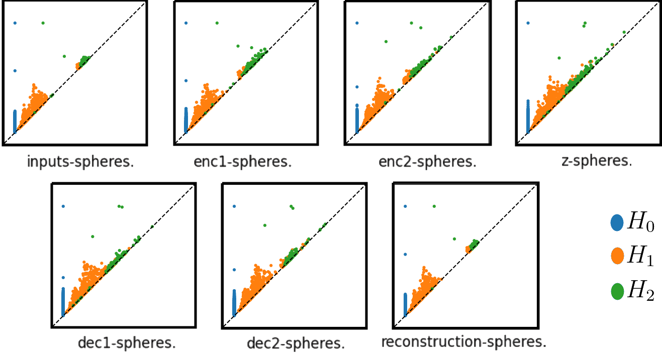
Figure 1: Example of data from Experiment 2: for each autoencoder layer, we plot the corresponding PD for $H_{0},H_{1},H_{2}$, in order from the input layer (left, first line) to the output/reconstruction layer (right, second line), for a total of $7$ layers. We plot the distance of each persistence diagram to the first one with respect to different metrics in Fig. 2.

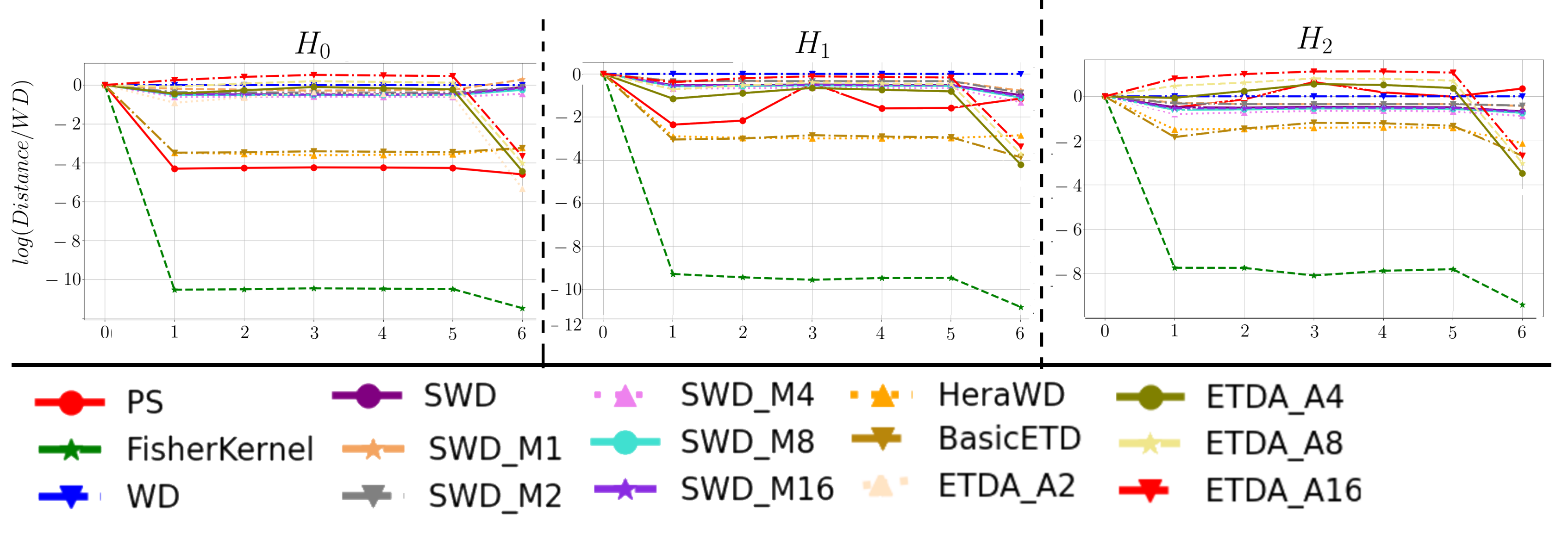
Figure 2: Example data from Experiment 2: we plot, for each homology dimension $0,1,2$, the values of $\log(\mathsf{dist}(P_{i},P_{0})/\mathsf{WD}(P_{i},P_{0})),0\leq i\leq 6$ where $P_{i}$ is the PD of the $i$-th layer, and $\mathsf{dist}$ is amongst our allowed metrics. For completeness, we also include the Fisher Kernel distance comparison, which is much less discriminative than other metrics.

Interpretation of the results. Qualitative observation of topological curves as in Figure 2 across several experiments indicates that PS eliminates all variations at the level of $0$th homology group $H_{0}$, and introduces large variations for successive homology groups, whereas the other more precise metrics indicate lower variations. This indicates high unreliability for $PS$ metrics on qualitative tasks. We see agreement in the overall diagram shapes between $W_{2}$ curves, $SW_{2}$ curves, and $\mathsf{ETD}_{A_{i}}$ curves for varying values of $i$, which may be due to relative normalization factors between the metrics. Recall that as $i$ increases, in theory, due to (6), we expect that $\mathsf{ETD}_{A_{i}}$ become more accurate because it approximates SW distance more closely. We observe that the $\mathsf{ETD}_{A_{i}}$ curves generally diminish their oscillations as $i$ increases, with topological curve shapes similar to the one for Wasserstein distance (see Figure 2). Table 3 shows time in seconds for computing such curves.

Distance	Time in milliseconds
	Autoencoder Weight Topology		Supervised Learning
	RELU	LRELU	Outex
WD	12544.96	13626.25	459.24
SWD	1588.80	1551.46	404.09
Hera WD	5816.86	6574.51	864.83
$ETD_{A_{1}}$	3.69	3.77	4.19
$ETD_{A_{2}}$	88.24	72.17	8.55
$ETD_{A_{4}}$	118.87	135.30	17.11
$ETD_{A_{8}}$	236.52	271.12	34.43
$ETD_{A_{16}}$	469.74	545.9890	69.11
$PS$	18.61	17.53	7.51

Table 3: Average time of each distance in milliseconds spanned by activation function and by datasets on the autoencoder and supervised learning experiments respectively.

We also tested the case of $\mathsf{SWD}$ metric with a number of slices of $a=1,2,4,8,16$ versus the corresponding $ETD_{A}$ distances with $\#A=a$, and obtained that the best computational time improvement of $\mathsf{ETD}_{A}$ versus $\mathsf{SWD}$ is for low values of $a=\#A$: we obtain respectively an improvement by a factor of $19.4,1.29,1.21,1.1,1.1$ for the values of $a=1,2,4,8,16$ for trials of our autoencoder tasks from Experiment 2. This means that our implementation is more time-efficient than $\mathsf{SWD}$ by these factors even when applying an equal number of slices, provided this value is relatively low.

5 Conclusion

We have introduced a new class of distances $\mathsf{ETD}_{A}$ on PDs for varying small parameter set $A$. These distances on the one hand may extend the distance between vectorizations used as the basis of Persistence Statistics, and on the other hand can in theory be enriched (at the cost of increasing $A$) to approximate Sliced Wasserstein Distance between PDs. In the low-$\#A$ range considered here, $\mathsf{ETD}_{A}$ pseudodistance computation has theoretical complexity bounds lower than previous distances, with no additional overhead time cost (contrary to most performant WD approximations which require to construct extra data structures with an overhead to the theoretical computational cost). The cost of $\mathsf{ETD}_{A}$ for low number of angles $\#A$ turns out to be only marginally higher than the simpler PS-based metrics, and for $A_{1}$ (“basic ETD" case) it is actually substantially lower than for PS due to optimizations specific to this case (see discussion after Def. 2). In practice, computational time for ETDs is considerably lower than state-of-art versions of WD or SWD distances. At the same time, in terms of accuracy loss, when tested on several common ML pipelines based on PDs, we see that ETD has higher performance than PS, and competitive accuracy performance compared to WD and SWD on ML tasks, since with ETD we reach similar qualitative description as with WD/SWD in Experiment 2, while PS-metrics seem to have unreliable qualitative behavior. Thus while having no strong theoretical guarantees of accuracy, the loss of accuracy of $\mathsf{ETD}_{A}$, even for for low values of $\#A$, seems to be minimal compared to finer distances such as WD or SWD distances.

In the comparison of our new implementation to SWD with equal numbers of slices, we find that having been careful with diagonal projections of the PD’s allows notable gains for very low values of these numbers of slices (especially $a=1,2,4$) compared to SWD. These are values of major interest in our experiments, for which we find a qualitative gain of accuracy in our tasks.

In summary we find that $\mathsf{ETD}_{A}$-distances allow a compromise between low computational time and low accuracy losses, allowing to interpolate between accurate WD or SWD metrics and simple PS-based metrics, by changing an in-built complexity parameter $\#A$. Furthermore, several possibly task-specific modifications presented in Appendix B can allow further adaptation of these distances to specific tasks. We expect that the theoretical control as well as experimentation with a wider variety of tasks will be a fruitful future avenue of research.

Appendix A Proofs of theoretical results

A.1 Proof of Lemma 1

It suffices to consider a point $(b_{i},d_{i})$: applying the projections from the statement of the lemma, we get

$$\pi_{0}(b_{i},d_{i}) = b_{i},$$

$$\pi_{\pi/2}(b_{i},d_{i}) = d_{i},$$

$$\pi_{\pi/4}(b_{i},d_{i}) = \frac{\sqrt{2}}{2}(b_{i}+d_{i}),$$

$$\pi_{3\pi/4}(b_{i},d_{i}) = \frac{\sqrt{2}}{2}(d_{i}-b_{i}).$$

Then the proof of the lemma follows by direct rescaling and comparison to (3).

A.2 Proof of Theorem 1

In order to compute $\mathsf{ETD}_{A}(\mathsf{P}_{1},\mathsf{P}_{2})$ we need to calculate the $k+1$ distances $D_{j}^{A}(\mathsf{P}_{1}^{j},\mathsf{P}_{2}^{j})$ and for each of them we need to compute $\#A$ terms of the form $W_{p}(\pi_{\theta}(\mathsf{P}_{1}^{j}\cup\widetilde{P}_{2}^{j}),\pi_{\theta}(\mathsf{P}_{2}^{j}\cup\widetilde{P}_{1}^{j}))$. For each of these terms, the cardinality of $\mathsf{P}_{1}^{j}\cup\widetilde{P}_{2}^{j}$ and $\mathsf{P}_{2}^{j}\cup\widetilde{P}_{1}^{j}$ is bounded above by $M$ and the computation of $\pi_{\theta}$ then requires to compute $\sin\theta,\cos\theta$ once, and then the computation of at most $M$ terms of the form $b_{i}\cos\theta+d_{i}\sin\theta$, requiring $3$ operation each. The calculation of $W_{p}$ using the formula given in Def. 2, requires to sort vectors of cardinality at most $M$, which takes at most $M\log M$ operations, and then to calculate the power $p$ of the $\ell_{p}$-norm of the difference, which takes $M$ operations of taking $p$-th power and $M-1$ operation of sum. Then we require $k(\sharp A-1)$ more sum operations and an operation of $1/p$-th power. Summing all these operations gives the first claimed bound from the theorem’s statement. As $T_{1},T_{2}$ are fixed constants, we directly get the $O(\cdots)$-based bound.

A.3 Justification of Equation (6)

We observe that, from Def. 2, we get

$$\frac{1}{n}D_{j}^{A_{n}}(\mathsf{P}_{1},\mathsf{P}_{2})^{p}=\frac{1}{n}\sum_{i=0}^{n-1}W_{p}(\pi_{\theta_{i}}(\mathsf{S}_{1}),\pi_{\theta_{i}}(\mathsf{S}_{2}))^{p}.$$

In the above, we denoted for simplicity $\mathsf{S}_{1}:=\mathsf{P}_{1}^{j}\cup\widetilde{P}_{2}^{j}$ and $\mathsf{S}_{2}:=\mathsf{P}_{2}^{j}\cup\widetilde{P}_{1}^{j}$, and also $A_{n}=\{\theta_{i}:\ 0\leq i<n\}$. Note that due to the definition (5) of $A_{n}$ the values $\theta_{i}$ are $n$ equally spaced points in the interval $[0,\pi)$. It is then direct to check that the last displayed formula is actually a Riemann sum approximation of

$$\frac{1}{\pi}\int_{0}^{\pi}W_{p}(\pi_{\theta}(\mathsf{S}_{1}),\pi_{\theta}(\mathsf{S}_{2}))^{p}d\theta=SW_{p}(\mathsf{P}_{1}^{j},\mathsf{P}_{2}^{j})^{p},$$

and the classical Riemann integral approximation theorem gives the desired result.

A.4 Details about stability control with $\mathsf{ETD}_{A_{n}}$

The classical result Chazal et al. [2009], Cohen-Steiner et al. [2010b] is that if for $X_{1},X_{2}$ finite metric spaces, the $j$-dimensional PDs $\mathsf{P}_{1},\mathsf{P}_{2}$ are obtained from the Rips complex, then

$$W_{\infty}(\mathsf{P}_{1},\mathsf{P}_{2})\leq GH(X_{1},X_{2}),$$

in which $GH$ is the Gromov-Hausdorff distance (see e.g. [Burago et al., 2022, Ch.7]). Next, from e.g. [Atienza et al., 2020, Lem. 3.5] we have the observation, based on a similar result for $\ell_{p},\ell_{\infty}$ norms, that $W_{p}$ is controlled by $W_{\infty}$, however this is comes at the cost of including a dependence on $M:=\#\mathsf{P}_{1}+\#\mathsf{P}_{2}$, for the most interestig lower bound (we include the upper bound for completenes but we do not use it):

$$M^{-1/p}W_{p}(\mathsf{P}_{1},\mathsf{P}_{2})\leq W_{\infty}(\mathsf{P}_{1},\mathsf{P}_{2})\leq W_{p}(\mathsf{P}_{1},\mathsf{P}_{2}).$$

Using (7) in conjunction with the above lower bounds, we then obtain a stability control on $SW_{p}$ as well, and via (6) we obtain bounds for $\mathsf{ETD}_{A_{n}}$ for large $n$. Note that at the moment these bounds are somehow weak, due to the limit in (6) and to the dependence on $M$ in the above $W_{p}/W_{\infty}$ bound. Thus we focused on experimental comparisons of $\mathsf{ETD}_{A}$ for small values of $\#A$, and leave this theoretical comparison to future work.

Appendix B Possible ad-hoc modifications for ETDs

In applications, there may be a series of minor modifications to the initial ETD definition (Def. 2) that users may want to implement for specific tasks. We list a list of such possible modifications here.

B.1 Dimensional reweighting

It may be useful to include ad-hoc normalization weights $w=(w_{0},\dots,w_{k})$ with $w_{j}>0$, for the auxiliary distances $D_{j}^{A},j=0,\dots,k$ in Def. 2, and define

$$\mathsf{ETD}_{A}^{w}(\mathsf{P}_{1},\mathsf{P}_{2}):=\left(\sum_{j=0}^{k}w_{j}D_{j}^{A}(\mathsf{P}_{1}^{j},\mathsf{P}_{2}^{j})^{p}\right)^{1/p}.$$

The usefulness of such weights (which can be hyperparameters or learned parameters in a ML task) depends of relative relevance of different types of topological features for given tasks.

B.2 Dimension-dependent angle choices

It may be useful to let the choice of angle sets $A$ depend upon dimension $j$, rather than being fixed as in Def. 2. This means that we fix sets $A_{0},\dots,A_{j}\subset[0,2\pi)$ and in Def. 2 replace $D_{j}^{A}$ by

$$D_{j}^{A_{j}}(\mathsf{P}_{1}^{j},\mathsf{P}_{2}^{j}):=\left(\sum_{\theta\in A_{j}}W_{p}(\pi_{\theta}(\mathsf{P}_{1}^{j}),\pi_{\theta}(\mathsf{P}_{2}^{j}))^{p}\right)^{1/p}.$$

A special case of these changes is mentioned immediately after Def. 2: if $\mathsf{P}^{0}$ has by construction birth coordinates $b=0$, then it is useful to only consider the death coordinates $d$, i.e. to use $A_{1}=\{\pi/2\}$. The natural choices for $A_{j}$ are given in (5).

B.3 Randomization

A common strategy for dimension reduction endeavors such as the passage from WD to SWD often profit from the use of randomized projections, akin to the framework of the Johnson-Lindenstrauss theorem. This has been implemented in Deshpande et al. [2019], Nietert et al. [2022], Nadjahi et al. [2021] for classical SWD optimization for point clouds in large dimension. Choosing randomized projection for the dimension reduction from $2$ to $1$ dimensional multisets in our framework, will give minimal computational time gains compared no fixing the $A_{n}$ as above. Furthermore, theoretical convergence rate in the approximation to $SW_{p}$ like (6) is reduced for randomized $A_{n}$.

B.4 1-dimensional Wasserstein alternatives with general metrics replacing $\ell_{p}$-norm

In some applications such as word2vec vectorizations, other metrics for comparing vectorizations are used, besides classical Banach space norms. This can be adapted to the present framework. For example, to compare accuracy values for $A=A_{n}$ as in (5), besides using $EDT_{A}$ with based on $W_{p}(\mathsf{S}_{1},\mathsf{S}_{2})=\|\mathsf{sort}(\mathsf{S}_{1})-\mathsf{sort}(\mathsf{S}_{2})\|_{\ell_{p}}$ as in Definition 2, one may try out different distances instead of $\ell_{p}$, in order to compare the vectors $V_{i}:=\mathsf{sort}(\mathsf{S}_{i})$, for example cosine similarity corresponding to taking a scalar product of the vectors:

$$d_{\cos}(V_{1},V_{2}):=\left|\sum_{i}(V_{1})_{i}(V_{2})_{i}\right|.$$

We sum these distances over $\theta\in A_{n}$ as in Definition 2 as an alternative to our $\mathsf{EDT}_{A_{n}}$. While the mathematical grounding for these alternative definitions is less strong than for the canonical version in Def. 2, it may be worth to try such alternatives for experimental evaluation on ad-hoc tasks.

Appendix C Implementation details

Algorithm 1 $get\_L\_vector$: Computes the $\mathcal{L}$ vector.

Input: A persistence diagram $\mathsf{P}$.
Output: The longevity vector $L$ of $\mathsf{P}$.

1:  $k\leftarrow|\mathsf{P}|$, $L\leftarrow()$, $j\leftarrow 0$

2:  for $j\leq k$ do

3:     $L_{j}\leftarrow()$

4:     for $(b,d)\leq\mathsf{P}^{j}$ do

5:        $L_{j}.add(d-b)$

6:     end for

7:     $L_{j}\leftarrow\mathsf{sort}(L_{j})$

8:     $L.add(L_{j})$

9:     $j\leftarrow j+1$

10:  end for

11:  return  $L$

Algorithm 2 $get\_V\_vector$: Computes the $\mathcal{L}$ vector.

Input: A persistence diagram $\mathsf{P}$ and an angle $\alpha$.
Output: The $V$ vector of $\mathsf{P}$ associated to $\alpha$.

1:  $k\leftarrow|\mathsf{P}|$, $V\leftarrow()$, $j\leftarrow 0$

2:  $(b_{\alpha},d_{\alpha})\leftarrow(cos(\alpha),sin(\alpha))$

3:  for $j\leq k$ do

4:     $V_{j}\leftarrow()$

5:     for $(b,d)\leq\mathsf{P}^{j}$ do

6:        $v_{j}\leftarrow b\cdot b_{\alpha}+d\cdot d_{\alpha}$

7:        $V_{j}.add(v_{j})$

8:     end for

9:     $V_{j}\leftarrow\mathsf{sort}(V_{j})$

10:     $V.add(V_{j})$

11:     $j\leftarrow j+1$

12:  end for

13:  return  $V$

Algorithm 3 $BasicETD$: Computes the $ETD_{A_{1}}$ pseudodistance.

Input: Two persistence diagrams $\mathsf{P}_{1},\mathsf{P}_{2}$ and a power value $p$.
Output: The basic ETD pseudodistance between $\mathsf{P}_{1},\mathsf{P}_{2}$.

1:  $L_{1}\leftarrow get\_L\_vector(\mathsf{P}_{1})$

2:  $L_{2}\leftarrow get\_L\_vector(\mathsf{P}_{2})$

3:  $L_{1}^{\prime},L_{2}^{\prime}\leftarrow padding\_zeroes(L_{1},L_{2})$

4:  $k\leftarrow|L_{1}^{\prime}|$

5:  return  $\lVert L_{1}^{\prime}-L_{2}^{\prime}\rVert_{p}$

Algorithm 4 $ETD_{A}$: Computes the $ETD_{A}$ pseudodistance.

Input: Two persistence diagrams $\mathsf{P}_{1},\mathsf{P}_{2}$, and angle set $A$ and a power value $p$.
Parameter: Optionally $\widetilde{P}_{1},\widetilde{P}_{2}$ can be precomputed.
Output: The $ETD_{A}$ pseudodistance between $\mathsf{P}_{1},\mathsf{P}_{2}$ considering $A$.

1:  $E\leftarrow()$

2:  if  $\widetilde{P}_{1}=\emptyset$  then

3:     $\widetilde{P}_{1}^{j}\leftarrow\{((b+d)/2,(b+d)/2):\ (b,d)\in\mathsf{P}_{1}^{j}\}$

4:  end if

5:  if  $\widetilde{P}_{2}=\emptyset$  then

6:     $\widetilde{P}_{2}^{j}\leftarrow\{((b+d)/2,(b+d)/2):\ (b,d)\in\mathsf{P}_{2}^{j}\}$

7:  end if

8:  $\mathsf{P}_{1}.extend(\widetilde{P}_{2})$ {dimension-wise concatenation}

9:  $\mathsf{P}_{2}.extend(\widetilde{P}_{1})$

10:  for $\alpha\in A$ do

11:     $V_{1}\leftarrow get\_V\_vector(\mathsf{P}_{1},\alpha)$

12:     $V_{2}\leftarrow get\_V\_vector(\mathsf{P}_{2},\alpha)$

13:     $etd_{\alpha}\leftarrow\lVert V_{1}-V_{2}\rVert_{p}^{p}$

14:     $E.add(etd_{\alpha})$

15:  end for

16:  return  $\lVert E\rVert_{p}$

Algorithm 3 and Algorithm 4 depends on the implementation of $L,V$ vectors and projections to the diagonal. We used a naive implementation of these methods in our experiments, but these results can be enhanced using more sophisticated libraries Numpy, PyTorch, TensorFlow, GPU kernels or python multiprocessing libraries. To demonstrate this potential, we have developed a prototype implementation utilizing Numpy Harris et al. [2020], which achieves considerable speed ups in computing these functions, and therefore the ETDs.

⬇

1import numpy as np

2

3def get_L_vector(PD):

4 longevity = []

5 hgroups = len(PD)

6 for d in range(hgroups):

7 # persistence computation

8 dlongevity = np.diff(PD[d], axis=1).T

9 # numpy descending sorting

10 dlongevity[0][::-1].sort()

11

12 longevity.append(dlongevity[0])

13

14 return longevity

15

16def get_V_vector(PD, alpha):

17 if alpha is None:

18 return ExtendedTopologyDistanceHelper.get_L_vector(PD)

19

20 alpha_interval = np.array([np.cos(alpha), np.sin(alpha)])

21 longevity = []

22 hgroups = len(PD)

23

24 for d in range(hgroups):

25 dlongevity = PD[d] @ alpha_interval

26 dlongevity[::-1].sort()

27 longevity.append(dlongevity)

28

29 return longevity

30

31def get_maximum_sizes(PDs):

32 max_sizes = {}

33 for PD in PDs:

34 for j, PDj in enumerate(PD):

35 hgcard = len(PDj)

36 if d not in max_sizes: # missing dimension

37 max_sizes.update({d: hgcard})

38 if max_sizes[d] < hgcard:

39 max_sizes[d] = hgcard

40 return max_sizes

41

42def padding_zeroes(PD1, PD2):

43 max_sizes = get_maximum_sizes([PD1, PD2])

44

45 AA = []

46 BB = []

47 siA = len(A)

48 siB = len(B)

49

50 for d in max_sizes:

51 padded = np.zeros(max_sizes[d])

52 padded2 = np.zeros(max_sizes[d])

53 if siA > d:

54 padded[:len(A[d])] = A[d]

55 if siB > d:

56 padded2[:len(B[d])] = B[d]

57

58 AA.append(padded)

59 BB.append(padded2)

60

61 return AA, BB

62

63def get_projection(PD):

64 mvect = []

65 max_dim = len(PD)

66 for d in range(max_dim):

67 mid = np.sum(PD[d], axis = 1)*0.5

68

69 mvect.append(np.vstack((mid, mid)).T)

70

71 return mvect

In Harris et al. [2020] there is an exposition on the diverse Numpy capabilities for array programming (including a) data structures, b) indexing, c) vectorization, d) broadcasting and e) reductions (illustrated in Figure 1 of Harris et al. [2020]). Its foundational role underpins numerous numerical computation libraries, and its influence extends to the core of Machine Learning and Deep Learning tools such as PyTorch and TensorFlow, which adopt a Numpy-like syntax. This compatibility ensures a seamless transition of code between Numpy and these frameworks, enabling almost direct mapping of implementations.

The benefits of adopting these Numpy-enhanced functions are evident in our extended experiments, which are documented with the ‘np’ prefix in Table 5 within Appendix D, and in Table 6 found in Appendix E. The source code of this paper is available in http://github.com/rolan2kn/aaai2024_etd_src.

Appendix D Extended Supervised Learning experiment

We extends our experiments of Section 4.1 on Supervised Learning to Shrec07 Giorgi et al. [2008] and Fashion-MNIST Xiao et al. [2017b].

D.1 Dataset Description

The aim of the Shrec07 dataset Giorgi et al. [2008] was to provide a common benchmark for the evaluation of the effectiveness of 3D-shape retrieval algorithms. The dataset consists of 400 OFF format files, encoding meshes of 3D surfaces without defective holes or gaps, subdivided into 19 classes of 20 elements each, shown in Figure 3(a). Note that the meshes have highly varying sizes, even within the same class. As explained in Section D.3, we use Shrec07 in a supervised learning task by splitting the dataset into train and test sets.

Fashion-MNIST Xiao et al. [2017b] is a dataset consisting of 28x28 grayscale article images, labelled according to 10 possible classes, and origined from a fashion retailer’s article images. The dataset consists of a training set of 60000 examples and a test set of 10000 examples.

(a) The Shrec’07 dataset from Giorgi et al. [2008]. Note that compared to the original case, the "spring" class (row 7 from the bottom) was removed in our experiment, as the examples in this class are not topologically consistent.

(b) The fashion mnist dataset divided into class examples.

Figure 3: Datasets

D.2 Data preprocessing

For the Shrec07 dataset, we compute persistence diagrams on each mesh-sample and create a new dataset composed with obtained the persistence diagrams. Then, using our proposed distances and kernels, we assess the classifiers. Each Shrec07 example is a mesh object stored in an OFF (Object File Format) file, from which we extract the 3D points ignoring edges and faces. Then we compute a 3D Heat Kernel Signature (HKS) Zobel et al. [2011] and produce a 6-dimensional embedding by concatenating HKS coordinates with mesh vertex coordinates. Then we build an associated sparse Rips complex up to $H_{2}$. In order to get possibly better results, one could have considered a filtration via different HKS’s depending of a parameter value: we did not do this due to time constraints, as it would be computationally intensive.

For the Fashion-MNIST setting, we adopt a preprocessing stage where on every image we apply the Histogram of Oriented Gradients (HOG) operator Dalal and Triggs [2005]. The process includes global image normalization, computing the gradient image in row and col (8 orientations), computing gradient histograms (8x8 pixels per block), normalizing across blocks (2x2 cells per block), and flattening image $i$ into a feature vector $i_{f}$. Finally the obtained feature vector is normalized as $i_{s}=\frac{i_{f}-mean(i_{f})}{\sigma(i_{f})}$.

D.3 Results

We formulate the Shrec07 dataset classification task as follows. We randomly select 15 examples per class, for a total of 285 examples, and for the test set we sample 10 of the 95 remaining files.

On Fashion-MNIST dataset, we use 1000 samples as train set (100 per class) and again 10 samples as test set. Table 4 shows the accuracy obtained with these tasks. Table 5 shows the average time in milliseconds that takes compute one of such distances. We use a laptop Acer Aspire A315-42 with 32 GB RAM, and an AMD Radeon vega 10 graphics.

Distance ($H_{1}$)	Shrec07		Fashion-MNIST
	Accuracy	k	Accuracy	k
$WD$	0.9	1-6,10,13	0.6	8,10,14-17,22,23
$Hera\_WD$	0.5		0.7	6,10
$SWD_{a=1}$	0.6	2-4	0.4	1,2,8-29
$SWD_{a=2}$	0.6	2-4	0.5	4,11,
$SWD_{a=4}$	0.6	2,9,10	0.6	2,3,5,8-11,
$SWD_{a=8}$	0.6	2,6-14	0.7	6
$SWD_{a=16}$	0.5	1-4,9,10,12	0.6	3,6
$ETD_{A_{1}}$	0.8	1-4	0.7	4,5
$ETD_{A_{2}}$	0.8	1-4	0.7	4,5,
$ETD_{A_{4}}$	0.8	1,7,8	0.7	8-29
$ETD_{A_{8}}$	0.9	2,7,8	0.7	6,10-13,16-29
$ETD_{A_{16}}$	0.9	7,8	0.6	8-29
$PS$	0.4	3,4	0.5	9,12,13,21,29
Fisher Kernel	0.5	5,8,10	0.4	24-41

Table 4: Accuracy of datasets using KNN with the respective k values.

Distance	Time in milliseconds
	Supervised Learning
	Shrec07	Fashion-MNIST
$WD$	305774.22	4794.9476
$Hera\_WD$	46372.22	4042.86
$SWD_{a=1}$	127.26	17.74
$SWD_{a=2}$	199.33	386.58
$SWD_{a=4}$	331.42	48.54
$SWD_{a=8}$	617.25	90.59
$SWD_{a=16}$	1184.80	173.90
$ETD_{A_{1}}$	12.34	1.48
$ETD_{A_{2}}$	132.19	24.68
$ETD_{A_{4}}$	251.71	46.78
$ETD_{A_{8}}$	490.11	90.79
$ETD_{A_{16}}$	967.94	178.66
$npETD_{A_{1}}$	0.77	0.06
$npETD_{A_{2}}$	8.36	0.62
$npETD_{A_{4}}$	17.67	1.10
$npETD_{A_{8}}$	35.97	2.14
$npETD_{A_{16}}$	72.95	4.24
$PS$	42.3	8.30
Fisher Kernel	12724.06	454.71

Table 5: Average times in milliseconds of a single distance computation in $H_{1}$.

As future work, in the case of Fashion-MNIST dataset, we plan to explore more sophisticated frameworks for classifying grayscale images such as Bergomi et al. [2019] and Garin and Tauzin [2019]. Both works apply different cubical filtrations to images to generate a wide range of topological features that leads to similar accuracy to more complex scenarios but with much lower number of features Bergomi et al. [2019]. These works were focused on applying vectorization methods included in Ali et al. [2023], which prevents them to be a perfect match for our tasks since we are operating directly on the persistence diagrams considering different distances. However, in Garin and Tauzin [2019], the authors use Wasserstein and Bottleneck amplitude, computed by calculating the $L_{2}$ norm of the persistence intervals, that is the L2-norm of unsorted vector $L$, multiplied by $\sqrt{2}/2$, similar to the $3\frac{3\pi}{4}$ projection) which is strictly less discriminative than our ETD, suggesting that we could obtain similar or better results.

Appendix E Extended autoencoder experiment

The concentric spheres are manifolds of dimension 99, and thus if densely sampled we expect to find 2 components at 0-dimensional homology level, and trivial homology in dimensions 1 and 2. As we use a sparse random sampling by of 2000 points, the induced topological errors are nontrivial. In Figures 4 and 5, we illustrate the latent spaces captured by our autoencoder and further elaborate on the Persistence Diagrams (PDs) for each layer, calculating up to the second homology group, $H_{2}$. These point clouds, being considerably dense, These point clouds, being considerably dense, made the calculation of persistence diagrams in dimensions greater than 1 a challenge, requiring the use of complex dispersed Rips. This was achieved by setting the 0.75 quantile of the Manhattan distance matrix as the upper limit for edge length, employing a sparsity factor of 0.5, and performing edge collapses primarily on the 1-skeleton before expanding to higher dimensions up to dimension $3$ to be sure we capture topological features in $H_{2}$. Additionally, in Table 6, we present the average computation times, expressed in milliseconds, for calculating a single distance. This includes a comparative analysis of the average times for both the $SWD$ and the $ETD$, utilizing an identical count of projections.

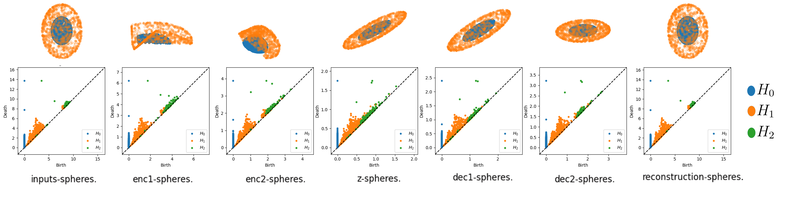
Figure 4: The Relu latent space information and persistence diagrams up to $H_{2}$.

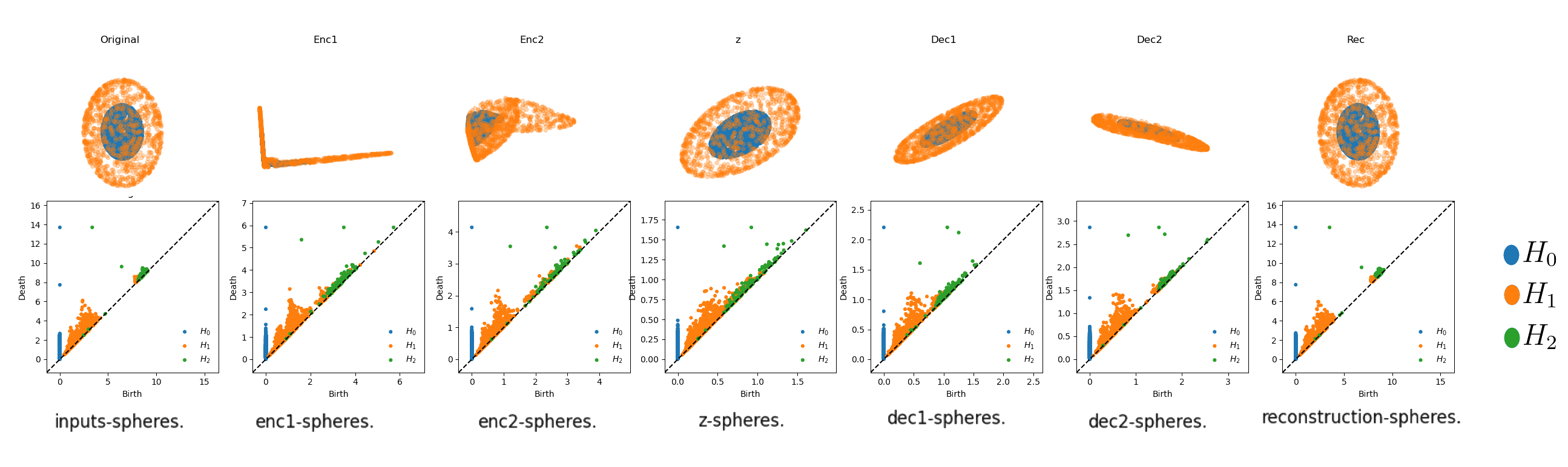
Figure 5: The LRelu latent space information and persistence diagrams up to $H_{2}$.

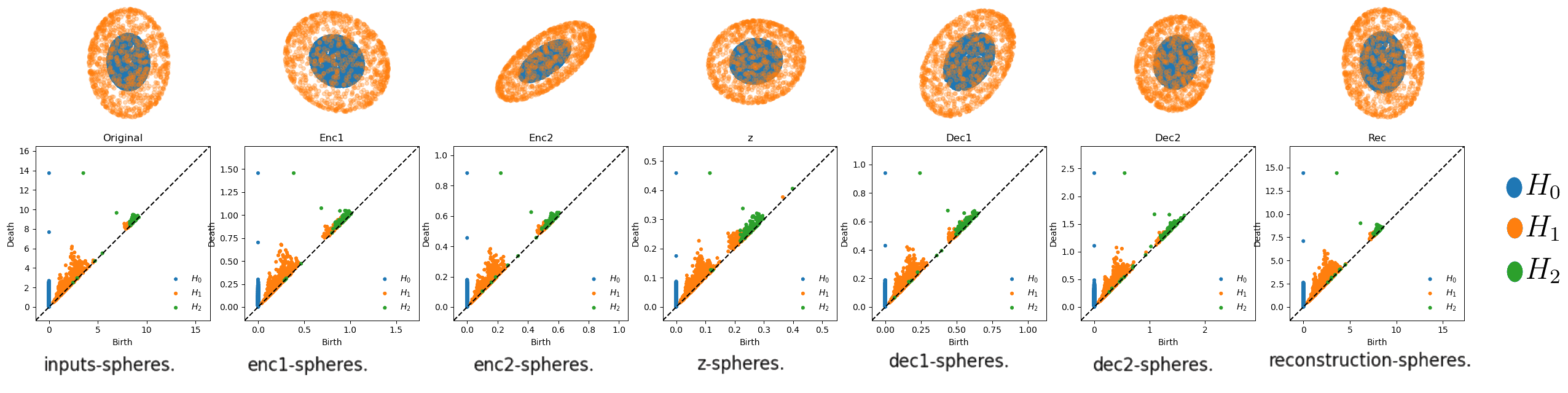
Figure 6: The Tanh latent space information and persistence diagrams up to $H_{2}$.

Distance	Time in milliseconds
	Autoencoder Weight Topology
	RELU	LRELU	Tanh
$WD$	20343.06	25488.97	16354.78
$Hera\_WD$	10484.34	13395.04	8896.01
$SWD_{a=1}$	70.33	97.41	67.34
$SWD_{a=2}$	119.31	160.05	104.52
$SWD_{a=4}$	201.45	257.90	186.33
$SWD_{a=8}$	388.60	519.23	347.73
$SWD_{a=16}$	706.65	956.24	655.33
$ETD_{A_{1}}$	6.00	4.89	3.85
$ETD_{A_{2}}$	78.75	87.12	125.15
$ETD_{A_{4}}$	142.59.45	165.19	136.57
$ETD_{A_{8}}$	306.30	344.08	272.24
$ETD_{A_{16}}$	630.02	732.73	570.31
$npETD_{A_{1}}$	3.46	4.77	4.70
$npETD_{A_{2}}$	2.00	2.78	1.75
$npETD_{A_{4}}$	3.11	4.27	2.71
$npETD_{A_{8}}$	6.19	8.44	5.33
$npETD_{A_{16}}$	12.43	16.91	9.71
$PS$	28.58	40.84	27.94
Fisher Kernel	3450.52	3526.64	3056.73

Table 6: Average time in milliseconds of computing a single distance in $H_{0},H_{1},H_{2}$, spanned by activation function and by datasets on the autoencoder experiment.

References

- Carlsson [2009] Gunnar Carlsson. Topology and data. Bull. Amer. Math. Soc., 46(2):255–308, 01 2009.
- Edelsbrunner and Harer [2010] Herbert Edelsbrunner and John Harer. Computational Topology - an Introduction. American Mathematical Society, 2010. ISBN 978-0-8218-4925-5. URL http://www.ams.org/bookstore-getitem/item=MBK-69.
- Cohen-Steiner et al. [2007] David Cohen-Steiner, Herbert Edelsbrunner, and John Harer. Stability of persistence diagrams. Discr. Comp. Geom., 37(1):103–120, 01 2007. ISSN 1432-0444. doi:10.1007/s00454-006-1276-5. URL https://doi.org/10.1007/s00454-006-1276-5.
- Cohen-Steiner et al. [2010a] David Cohen-Steiner, Herbert Edelsbrunner, John Harer, and Yuriy Mileyko. Lipschitz functions have lp-stable persistence. Found. Comp. Math., 10(2):127–139, 4 2010a. ISSN 1615-3383. doi:10.1007/s10208-010-9060-6. URL https://doi.org/10.1007/s10208-010-9060-6.
- Zomorodian [2009] Afra Zomorodian. Topology for Computing. Cambridge Monographs on Applied and Computational Mathematics. Cambridge University Press, 2009. ISBN 0521136091.
- Ghrist [2008] Robert Ghrist. Barcodes: The persistent topology of data. BULLETIN (New Series) OF THE AMERICAN MATHEMATICAL SOCIETY, 45:61–75, 02 2008. doi:10.1090/S0273-0979-07-01191-3.
- Seversky et al. [2016] Lee M. Seversky, Shelvi Davis, and Matthew Berger. On time-series topological data analysis: New data and opportunities. In 2016 IEEE Conference on Computer Vision and Pattern Recognition Workshops (CVPRW), pages 1014–1022, 06 2016. doi:10.1109/CVPRW.2016.131.
- Carr et al. [2017] Hamish Carr, Chistoph Garth, and Tino Weinkauf. Topological Methods in Data Analysis and Visualization IV. Theory, Algorithms, and Applications. Mathematics and Visualization. Springer International Publishing, 2017. ISBN 9783319446844. doi:10.1007/978-3-319-44684-4.
- Venkataraman et al. [2016] Vinay Venkataraman, Karthikeyan Natesan Ramamurthy, and Pavan K. Turaga. Persistent homology of attractors for action recognition. In ICIP 2016, pages 4150–4154, 2016. doi:10.1109/ICIP.2016.7533141. URL https://doi.org/10.1109/ICIP.2016.7533141.
- Umeda [2017] Yuhei Umeda. Time series classification via topological data analysis. Trans. Jap. Soc. AI, 32:D–G72, 05 2017. doi:10.1527/tjsai.D-G72.
- Wagner and Dłotko [2014] Hubert Wagner and Paweł Dłotko. Towards topological analysis of high-dimensional feature spaces. Comp. Vis. Im. Underst., 121:21–26, 2014. ISSN 1077-3142. doi:https://doi.org/10.1016/j.cviu.2014.01.005. URL https://www.sciencedirect.com/science/article/pii/S1077314214000125.
- Rawson et al. [2022] Michael Rawson, Samuel Dooley, Mithun Bharadwaj, and Rishabh Choudhary. Topological data analysis for word sense disambiguation, 2022. URL https://arxiv.org/abs/2203.00565.
- Kuhn et al. [2017] Alexander Kuhn, Wito Engelke, Markus Flatken, Hans-Christian Hege, and Ingrid Hotz. Topology-based analysis for multimodal atmospheric data of volcano eruptions. In Carr et al., editor, Topological Methods in Data Analysis and Visualization IV, pages 35–50. Springer, 2017. ISBN 978-3-319-44684-4.
- Sizemore et al. [2019] Ann E. Sizemore, Jennifer E. Phillips-Cremins, Robert Ghrist, and Danielle S. Bassett. The importance of the whole: Topological data analysis for the network neuroscientist. Network Neuroscience, 3(3):656–673, 2019. doi:10.1162/netn_a_00073. URL https://doi.org/10.1162/netn_a_00073.
- Lamar et al. [2016] Javier Lamar, Raul Alonso, Edel Garcia, and Rocio Gonzalez-Díaz. Persistent homology-based gait recognition robust to upper body variations. In ICPR2016, Cancún, Mexico, December 4-8, 2016, 2016.
- Hossny et al. [2016] Mostafa Hossny, Shady Mohammed, Saeid Nahavandi, Kyle Nelson, and Mo Hossny. Driving behaviour analysis using topological features. In SMC2016. IEEE, 2016.
- Garside et al. [2019] Kathryn Garside, Robin Henderson, Irina Makarenko, and Cristina Masoller. Topological data analysis of high resolution diabetic retinopathy images. PLOS ONE, 14(5):1–10, 05 2019. doi:10.1371/journal.pone.0217413. URL https://doi.org/10.1371/journal.pone.0217413.
- Ŝkraba [2018] Primoz Ŝkraba. Persistent homology and machine learning. Informatica, 42(2):253–258, 01 2018.
- Dobrushin [1970] R. L. Dobrushin. Prescribing a system of random variables by conditional distributions. Theory of Probability & Its Applications, 15(3):458–486, 1970. doi:10.1137/1115049. URL https://doi.org/10.1137/1115049.
- Panaretos and Zemel [2019] Victor M. Panaretos and Yoav Zemel. Statistical aspects of wasserstein distances. Annual Review of Statistics and Its Application, 6(1):405–431, 2019. doi:10.1146/annurev-statistics-030718-104938. URL https://doi.org/10.1146/annurev-statistics-030718-104938.
- Bubenik and Elchesen [2022] Peter Bubenik and Alex Elchesen. Universality of persistence diagrams and the bottleneck and wasserstein distances. Computational Geometry, 105-106:101882, 2022. ISSN 0925-7721. doi:https://doi.org/10.1016/j.comgeo.2022.101882. URL https://www.sciencedirect.com/science/article/pii/S0925772122000256.
- Munkres [1957] James Munkres. Algorithms for the assignment and transportation problems. Journal of the SIAM, 5(1):32–38, 2023/08/10/ 1957. ISSN 03684245. URL http://www.jstor.org/stable/2098689. Full publication date: Mar., 1957.
- Dey and Wang [2022] Tamal Krishna Dey and Yusu Wang. Computational topology for data analysis. Cambridge University Press, 2022.
- Kerber et al. [2017] Michael Kerber, Dmitriy Morozov, and Arnur Nigmetov. Geometry helps to compare persistence diagrams. ACM J. Exp. Algorithmics, 22, September 2017. ISSN 1084-6654. doi:10.1145/3064175.
- Chen and Wang [2021] Samantha Chen and Yusu Wang. Approximation algorithms for 1-wasserstein distance between persistence diagrams. In 19th Int. Symp. Exper. Alg., page 1, 2021.
- Backurs et al. [2020] Arturs Backurs, Yihe Dong, Piotr Indyk, Ilya Razenshteyn, and Tal Wagner. Scalable nearest neighbor search for optimal transport. In ICML, pages 497–506. PMLR, 2020.
- Carrière et al. [2017] Mathieu Carrière, Marco Cuturi, and Steve Oudot. Sliced Wasserstein kernel for persistence diagrams. In Doina Precup and Yee Whye Teh, editors, ICML, volume 70 of PMLR, pages 664–673. PMLR, 06–11 Aug 2017. URL https://proceedings.mlr.press/v70/carriere17a.html.
- Rabin et al. [2012] Julien Rabin, Gabriel Peyré, Julie Delon, and Marc Bernot. Wasserstein barycenter and its application to texture mixing. In Alfred M. Bruckstein, Bart M. ter Haar Romeny, Alexander M. Bronstein, and Michael M. Bronstein, editors, Scale Space and Variational Methods in Computer Vision, pages 435–446. Springer Berlin Heidelberg, 2012. ISBN 978-3-642-24785-9.
- Bonneel et al. [2015] Nicolas Bonneel, Julien Rabin, Gabriel Peyré, and Hanspeter Pfister. Sliced and radon wasserstein barycenters of measures. J. Math. Imaging and Vision, 51(1):22–45, 01 2015. ISSN 1573-7683. doi:10.1007/s10851-014-0506-3. URL https://doi.org/10.1007/s10851-014-0506-3.
- Paty and Cuturi [2019] François-Pierre Paty and Marco Cuturi. Subspace robust wasserstein distances. In ICML, pages 5072–5081. PMLR, May 2019. URL https://proceedings.mlr.press/v97/paty19a.html. ISSN: 2640-3498.
- Bayraktar and Guo [2021] Erhan Bayraktar and Gaoyue Guo. Strong equivalence between metrics of Wasserstein type. Electronic Communications in Probability, 26(none):1–13, January 2021. ISSN 1083-589X, 1083-589X. doi:10.1214/21-ECP383. URL https://projecteuclid.org/journals/electronic-communications-in-probability/volume-26/issue-none/Strong-equivalence-between-metrics-of-Wasserstein-type/10.1214/21-ECP383.full. Publisher: Institute of Mathematical Statistics and Bernoulli Society.
- Cuturi [2013] Marco Cuturi. Sinkhorn Distances: Lightspeed Computation of Optimal Transport. In NIPS, volume 26. Curran Associates, Inc., 2013. URL https://proceedings.neurips.cc/paper/2013/hash/af21d0c97db2e27e13572cbf59eb343d-Abstract.html.
- Chakrabarty and Khanna [2021] Deeparnab Chakrabarty and Sanjeev Khanna. Better and simpler error analysis of the sinkhorn–knopp algorithm for matrix scaling. Mathematical Programming, 188(1):395–407, 2021.
- Khrulkov and Oseledets [2018] Valentin Khrulkov and I. Oseledets. Geometry score: A method for comparing generative adversarial networks. In ICML, 2018.
- Dey and Zhang [2022] Tamal K. Dey and Simon Zhang. Approximating 1-Wasserstein Distance between Persistence Diagrams by Graph Sparsification, pages 169–183. Society for Industrial and Applied Mathematics, 2022. doi:10.1137/1.9781611977042.14. URL https://epubs.siam.org/doi/abs/10.1137/1.9781611977042.14.
- Adams et al. [2017] Henry Adams, Tegan Emerson, Michael Kirby, Rachel Neville, Chris Peterson, Patrick Shipman, Sofya Chepushtanova, Eric Hanson, Francis Motta, and Lori Ziegelmeier. Persistence images: A stable vector representation of persistent homology. JMLR, 18(8):1–35, 2017. URL http://jmlr.org/papers/v18/16-337.html.
- Ali et al. [2023] Dashti Ali, Aras Asaad, Maria-Jose Jimenez, Vidit Nanda, Eduardo Paluzo-Hidalgo, and Manuel Soriano-Trigueros. A survey of vectorization methods in topological data analysis. IEEE Trans. Patt. Anal. Mach.e Intell., pages 1–14, 2023. ISSN 1939-3539. doi:10.1109/TPAMI.2023.3308391.
- Chung and Lawson [2022] Yu-Min Chung and Austin Lawson. Persistence curves: A canonical framework for summarizing persistence diagrams. Advances in Computational Mathematics, 48(1):6, Jan 2022. ISSN 1572-9044. doi:10.1007/s10444-021-09893-4. URL https://doi.org/10.1007/s10444-021-09893-4.
- Fasy et al. [2020] Brittany Fasy, Yu Qin, Brian Summa, and Carola Wenk. Comparing distance metrics on vectorized persistence summaries. In TDA & Beyond, 2020. URL https://openreview.net/forum?id=X1bxKJo5_qL.
- Chazal et al. [2009] Frédéric Chazal, David Cohen-Steiner, Leonidas J. Guibas, Facundo Mémoli, and Steve Y. Oudot. Gromov-Hausdorff Stable Signatures for Shapes using Persistence. Computer Graphics Forum, 28(5):1393–1403, July 2009. ISSN 01677055, 14678659. doi:10.1111/j.1467-8659.2009.01516.x. URL https://onlinelibrary.wiley.com/doi/10.1111/j.1467-8659.2009.01516.x.
- Chazal et al. [2014] Frédéric Chazal, Vin de Silva, and Steve Oudot. Persistence stability for geometric complexes. Geometriae Dedicata, 173(1):193–214, December 2014. ISSN 1572-9168. doi:10.1007/s10711-013-9937-z. URL https://doi.org/10.1007/s10711-013-9937-z.
- Kuhn [1955] Harold W Kuhn. The hungarian method for the assignment problem. Nav. Res. Log. Quart., 2(1-2):83–97, 1955.
- Peyré et al. [2019] Gabriel Peyré, Marco Cuturi, et al. Computational optimal transport: With applications to data science. FTML, 11(5-6):355–607, 2019.
- Santambrogio [2015] Filippo Santambrogio. Optimal transport for applied mathematicians. Birkäuser, NY, 55(58-63):94, 2015.
- Horak et al. [2021] Danijela Horak, Simiao Yu, and Gholamreza Salimi-Khorshidi. Topology distance: A topology-based approach for evaluating generative adversarial networks. AAAI, 35(9):7721–7728, 05 2021. doi:10.1609/aaai.v35i9.16943.
- Chintakunta et al. [2015] Harish Chintakunta, Thanos Gentimis, Rocio Gonzalez-Diaz, Maria-Jose Jimenez, and Hamid Krim. An entropy-based persistence barcode. Pattern Recognition, 48(2):391–401, 2015.
- Bonnotte [2013] Nicolas Bonnotte. Unidimensional and evolution methods for optimal transportation. PhD thesis, Université Paris Sud-Paris XI; Scuola normale superiore (Pise, Italie), 2013.
- Nadjahi [2021] Kimia Nadjahi. Sliced-Wasserstein distance for large-scale machine learning : theory, methodology and extensions. Thesis, Institut Polytechnique de Paris, November 2021. URL https://theses.hal.science/tel-03533097.
- Atienza et al. [2020] Nieves Atienza, Rocío González-Díaz, and Manuel Soriano-Trigueros. On the stability of persistent entropy and new summary functions for topological data analysis. Pattern Recognition, 107:107509, 2020.
- Saul and Tralie [2019] Nathaniel Saul and Chris Tralie. Scikit-tda: Topological data analysis for python, 2019. URL https://doi.org/10.5281/zenodo.2533369.
- Flamary et al. [2021] Rémi Flamary, Nicolas Courty, Alexandre Gramfort, Mokhtar Z. Alaya, Aurélie Boisbunon, Stanislas Chambon, Laetitia Chapel, Adrien Corenflos, Kilian Fatras, Nemo Fournier, Léo Gautheron, Nathalie T.H. Gayraud, Hicham Janati, Alain Rakotomamonjy, Ievgen Redko, Antoine Rolet, Antony Schutz, Vivien Seguy, Danica J. Sutherland, Romain Tavenard, Alexander Tong, and Titouan Vayer. Pot: Python optimal transport. JMLR, 22(78):1–8, 2021. URL http://jmlr.org/papers/v22/20-451.html.
- Lacombe et al. [2018] Théo Lacombe, Marco Cuturi, and Steve Oudot. Large scale computation of means and clusters for persistence diagrams using optimal transport. In Proc. 32nd Int. Conference on Neural Information Processing Systems, NIPS’18, page 9792–9802. Curran Associates Inc., 2018.
- Maria et al. [2014] Clément Maria, Jean-Daniel Boissonnat, Marc Glisse, and Mariette Yvinec. The gudhi library: Simplicial complexes and persistent homology. In Hoon Hong and Chee Yap, editors, Mathematical Software – ICMS 2014. Springer Berlin Heidelberg, 2014.
- Ojala et al. [2002] T. Ojala, T. Maenpaa, M. Pietikainen, J. Viertola, J. Kyllonen, and S. Huovinen. Outex - new framework for empirical evaluation of texture analysis algorithms. In 2002 ICPR, volume 1, pages 701–706 vol.1, 8 2002. doi:10.1109/ICPR.2002.1044854.
- Pickup et al. [2016] D. Pickup, X. Sun, P. L. Rosin, R. R. Martin, Z. Cheng, Z. Lian, M. Aono, A. Ben Hamza, A. Bronstein, M. Bronstein, S. Bu, U. Castellani, S. Cheng, V. Garro, A. Giachetti, A. Godil, L. Isaia, J. Han, H. Johan, L. Lai, B. Li, C. Li, H. Li, R. Litman, X. Liu, Z. Liu, Y. Lu, L. Sun, G. Tam, A. Tatsuma, and J. Ye. Shape retrieval of non-rigid 3d human models. IJCV, 120(2):169–193, 11 2016. ISSN 1573-1405. doi:10.1007/s11263-016-0903-8. URL https://doi.org/10.1007/s11263-016-0903-8.
- Xiao et al. [2017a] Han Xiao, Kashif Rasul, and Roland Vollgraf. Fashion-mnist: a novel image dataset for benchmarking machine learning algorithms. CoRR, abs/1708.07747, 2017a. URL http://arxiv.org/abs/1708.07747.
- Kaczynski et al. [2004] T. Kaczynski, K. Mischaikow, and M. Mrozek. Computational Homology. Applied Mathematical Sciences. Springer New York, 2004. ISBN 9780387408538. URL https://books.google.cl/books?id=V1kyZ1E7pLgC.
- Wagner et al. [2011] Hubert Wagner, Chao Chen, and Erald Vuçini. Efficient computation of persistent homology for cubical data. In Topological methods in data analysis and visualization II: theory, algorithms, and applications, pages 91–106. Springer, 2011.
- Bergstra and Bengio [2012] James Bergstra and Yoshua Bengio. Random search for hyper-parameter optimization. JMLR, 13(Feb):281–305, 2012. ISSN ISSN 1533-7928. URL http://www.jmlr.org/papers/v13/bergstra12a.html.
- James et al. [2023] G. James, D. Witten, T. Hastie, R. Tibshirani, and J. Taylor. An Introduction to Statistical Learning: with Applications in Python. Springer Texts in Statistics. Springer, 2023. ISBN 9783031387470. URL https://books.google.cl/books?id=ygzJEAAAQBAJ.
- Pedregosa et al. [2012] Fabian Pedregosa, Gael Varoquaux, Alexandre Gramfort, Vincent Michel, Bertrand Thirion, Olivier Grisel, Mathieu Blondel, Peter Prettenhofer, Ron Weiss, Vincent Dubourg, Jake Vanderplas, Alexandre Passos, David Cournapeau, Matthieu Brucher, Matthieu Perrot, Edouard Duchesnay, and Gilles Louppe. Scikit-learn: Machine learning in python. JMLR, 12, 01 2012.
- Naitzat et al. [2020] Gregory Naitzat, Andrey Zhitnikov, and Lek-Heng Lim. Topology of deep neural networks. JMLR, 21(184):1–40, 2020. URL http://jmlr.org/papers/v21/20-345.html.
- Bengio et al. [2017] Yoshua Bengio, Ian Goodfellow, and Aaron Courville. Deep learning, volume 1. MIT press Cambridge, MA, USA, 2017.
- Cohen-Steiner et al. [2010b] David Cohen-Steiner, Herbert Edelsbrunner, John Harer, and Yuriy Mileyko. Lipschitz functions have l p-stable persistence. Found. Comp. Math., 10(2):127–139, 2010b.
- Burago et al. [2022] Dmitri Burago, Yuri Burago, and Sergei Ivanov. A course in metric geometry, volume 33. American Mathematical Society, 2022.
- Deshpande et al. [2019] Ishan Deshpande, Yuan-Ting Hu, Ruoyu Sun, Ayis Pyrros, Nasir Siddiqui, Sanmi Koyejo, Zhizhen Zhao, David Forsyth, and Alexander G Schwing. Max-sliced wasserstein distance and its use for gans. In Proceedings of the IEEE/CVF Conference on Computer Vision and Pattern Recognition, pages 10648–10656, 2019.
- Nietert et al. [2022] Sloan Nietert, Ziv Goldfeld, Ritwik Sadhu, and Kengo Kato. Statistical, robustness, and computational guarantees for sliced wasserstein distances. NeurIPS, 35:28179–28193, 2022.
- Nadjahi et al. [2021] Kimia Nadjahi, Alain Durmus, Pierre E Jacob, Roland Badeau, and Umut Simsekli. Fast Approximation of the Sliced-Wasserstein Distance Using Concentration of Random Projections. In Advances in Neural Information Processing Systems, volume 34, pages 12411–12424. Curran Associates, Inc., 2021. URL https://proceedings.neurips.cc/paper_files/paper/2021/hash/6786f3c62fbf9021694f6e51cc07fe3c-Abstract.html.
- Harris et al. [2020] Charles R. Harris, K. Jarrod Millman, Stéfan J. van der Walt, Ralf Gommers, Pauli Virtanen, David Cournapeau, Eric Wieser, Julian Taylor, Sebastian Berg, Nathaniel J. Smith, Robert Kern, Matti Picus, Stephan Hoyer, Marten H. van Kerkwijk, Matthew Brett, Allan Haldane, Jaime Fernández del Río, Mark Wiebe, Pearu Peterson, Pierre Gérard-Marchant, Kevin Sheppard, Tyler Reddy, Warren Weckesser, Hameer Abbasi, Christoph Gohlke, and Travis E. Oliphant. Array programming with NumPy. Nature, 585(7825):357–362, September 2020. doi:10.1038/s41586-020-2649-2. URL https://doi.org/10.1038/s41586-020-2649-2.
- Giorgi et al. [2008] Daniela Giorgi, Silvia Biasotti, and Laura Paraboschi. Shape retrieval contest 2007: Watertight models track. SHREC competition, 8, 07 2008.
- Xiao et al. [2017b] Han Xiao, Kashif Rasul, and Roland Vollgraf. Fashion-mnist: a novel image dataset for benchmarking machine learning algorithms, 2017b. URL http://arxiv.org/abs/1708.07747. cite arxiv:1708.07747Comment: Dataset is freely available at https://github.com/zalandoresearch/fashion-mnist Benchmark is available at http://fashion-mnist.s3-website.eu-central-1.amazonaws.com/.
- Zobel et al. [2011] Valentin Zobel, Jan Reininghaus, and Ingrid Hotz. Generalized heat kernel signatures. In International Conference in Central Europe on Computer Graphics and Visualization, 2011. URL https://api.semanticscholar.org/CorpusID:59453473.
- Dalal and Triggs [2005] N. Dalal and B. Triggs. Histograms of oriented gradients for human detection. In 2005 IEEE Computer Society Conference on Computer Vision and Pattern Recognition (CVPR’05), volume 1, pages 886–893 vol. 1, 2005. doi:10.1109/CVPR.2005.177.
- Bergomi et al. [2019] Mattia G. Bergomi, Patrizio Frosini, Daniela Giorgi, and Nicola Quercioli. Towards a topological–geometrical theory of group equivariant non-expansive operators for data analysis and machine learning. Nature Machine Intelligence, 1(9):423–433, Sep 2019. ISSN 2522-5839. doi:10.1038/s42256-019-0087-3. URL https://doi.org/10.1038/s42256-019-0087-3.
- Garin and Tauzin [2019] Adélie Garin and Guillaume Tauzin. A topological "reading" lesson: Classification of mnist using tda, 2019.