Diffusion Model Based Visual Compensation Guidance and Visual Difference Analysis for No-Reference Image Quality Assessment

Abstract

Existing free-energy guided No-Reference Image Quality Assessment (NR-IQA) methods still suffer from finding a balance between learning feature information at the pixel level of the image and capturing high-level feature information and the efficient utilization of the obtained high-level feature information remains a challenge. As a novel class of state-of-the-art (SOTA) generative model, the diffusion model exhibits the capability to model intricate relationships, enabling a comprehensive understanding of images and possessing a better learning of both high-level and low-level visual features. In view of these, we pioneer the exploration of the diffusion model into the domain of NR-IQA. Firstly, we devise a new diffusion restoration network that leverages the produced enhanced image and noise-containing images, incorporating nonlinear features obtained during the denoising process of the diffusion model, as high-level visual information. Secondly, two visual evaluation branches are designed to comprehensively analyze the obtained high-level feature information. These include the visual compensation guidance branch, grounded in the transformer architecture and noise embedding strategy, and the visual difference analysis branch, built on the ResNet architecture and the residual transposed attention block. Extensive experiments are conducted on seven public NR-IQA datasets, and the results demonstrate that the proposed model outperforms SOTA methods for NR-IQA.

I Introduction

With the rapid advancement of digital technologies, the growing significance of high-quality visual information has garnered widespread attention. To address the inevitable quality loss during the compression and transmission of visual data, image quality assessment (IQA) becomes crucial for ensuring the widespread dissemination of top-tier visual content. Categorized into subjective and objective IQA, the former relies on human perception, which is prone to biases and is resource-intensive. Objective IQA, particularly no-reference IQA (NR-IQA), emerges as a vital solution, employing computer algorithms for automatic image quality prediction. NR-IQA is particularly relevant in distorted scenarios without a reference image.

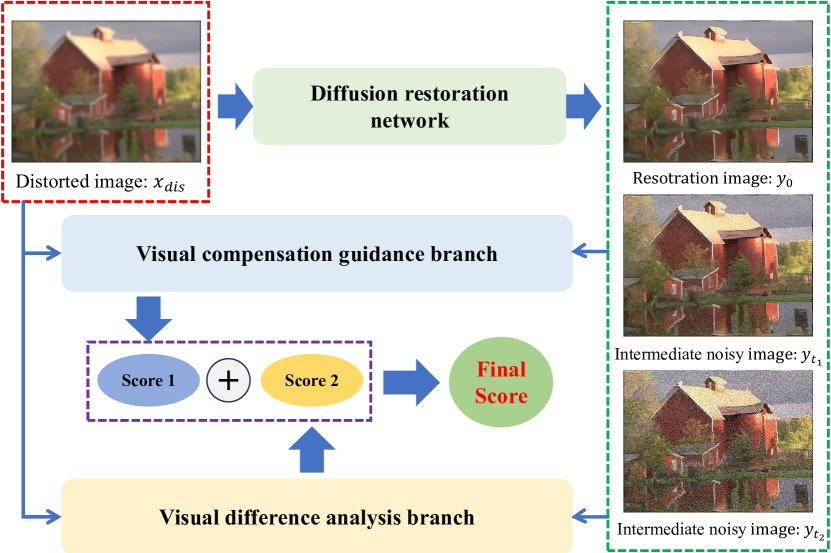
Figure 1: The overview framework of our proposed Diff$V^{2}$IQA model, which consists of two main components. The first part comprises a diffusion restoration network designed for image enhancement, while the second part involves a two-branch image quality evaluation network.

NR-IQA can be broadly categorized into two types based on the nature of image distortion: synthetic distortion and authentic distortion [1]. In synthetic distortion NR-IQA, intentionally generated low-quality data incorporates various distortions such as JPEG artifacts, contrast distortions, and blurring [2]. The resulting model primarily focuses on different distortion categories for the final evaluation and scoring. In an authentic distortion dataset, low-scoring images are not associated with specific distortions but rather with high-level image information, such as slightly blurry characters or poor overall composition [3, 4]. This introduces challenges, requiring the network to consider not only pixel-level image distortion but also prioritize high-level image information.

Early methods relied on hand-crafted features, broadly classified into two groups. One category [5, 6, 7, 8, 9] utilizes static features of the image for quality assessment, while the other [10, 11, 12, 13, 14] employs machine learning methods to understand the distribution of specific image features, mapping them to the final quality score. However, these methods have limitations and struggle to adequately characterize image features, facing challenges in accurately describing image properties for various types of distortion. With the advent of deep learning, especially convolutional neural networks (CNNs), some feature extraction methods based on CNN [15, 16, 17, 18, 19, 20, 21] have shown significant success in NR-IQA. These approaches leverage the inherent capability of convolution to autonomously extract crucial features from the image, significantly enhancing the precision of NR-IQA. As deep learning advances, researchers explore the integration of successful architectures from various domains into NR-IQA, such as architectures based on the free-energy principle [22, 23], graphical convolutional neural networks (GNN) [24], transformer-based architectures [25, 26, 27], contrast learning principle [28, 29], test-time adaptation strategy [30], and large language models [31, 32]. All these methodologies aim to improve the model’s ability to comprehend and analyze the image for a more precise quality score.

In [1], an extra network is used to enhance images. This network’s variables are utilized to improve the quality assessment, inspired by the idea that the human visual system has the inherent ability to automatically recover and improve images that have been distorted. However, this approach has limitations. Firstly, the chosen restoration network may need improvement in capturing both high-level and low-level information. Also, the features used for quality evaluations mainly consist of intermediate variables, lacking interpretability. Secondly, the high-level restoration features are underutilized, serving only as supplementary information for quality assessment. Thirdly, there is a need to enhance the master quality assessment network’s performance, focusing on refining the learning capabilities for pixel-level features. In [27], the use of the transformer architecture in NR-IQA is significantly advanced. They employ the vision transformer for feature extraction and leverage the swin transformer architecture to enhance the model’s acquisition of pixel-level features. However, the network lacks guidance from high-level image information, suggesting a potential avenue for performance improvement. Babnik et al. [33] pioneer the integration of diffusion modeling into facial IQA (FIQA), offering valuable theoretical insights and demonstrating the potential application of diffusion modeling in NR-IQA. However, it’s crucial to note that their FIQA task relies on reference images, and applying the diffusion model in a no-reference context remains a significant challenge.

To address the challenges outlined, we propose a novel image restoration network based on an enhanced diffusion model (see Fig. 1). The network leverages the final enhanced image and noise-containing images in the denoising process, providing superior interpretability compared to intermediate feature variables. To fully exploit high-level visual information, we introduce two evaluation branches: a visual compensation guidance branch and a visual difference analysis branch. The visual compensation guidance branch integrates high-level visual information with the original features of the distorted image for quality evaluation. It emphasizes the features of the distorted image, guided by high-level visual information. To enhance the model’s recognition of features, we employ a well-performing transformer architecture and introduce a new noise embedding strategy. This strategy improves the model’s ability to mine data features at different levels. The visual difference analysis branch focuses on learning the difference between the distorted image and the restored images, using ResNet as a feature extractor. A new RTAB module, based on the attention mechanism, improves differentiation learning. These two branches, with their distinct perspectives on high-level visual information, complement each other, aiding the network in quality evaluation.

In summary, the main contributions of our work are as follows:

• To the best of our knowledge, our work represents the first application of the diffusion model to the field of NR-IQA. Leveraging the free-energy principle, we devise a new diffusion image restoration model aimed at generating enhanced images as high-level visual features, which guide the master IQA network to obtain the final quality score.

• To fully exploit the rich high-level visual information introduced by the diffusion model, we design two visual evaluation branches. One concentrates on the intrinsic features of the distorted image, utilizing the higher-level image information as a visual compensation guidance. The second branch analyzes the differentiated information between the distorted image and the restored image. The culmination of these analyses results in a comprehensive final quality score.

• The proposed ‘Diffusion model based Visual compensation guidance and Visual difference analysis’ IQA network (Diff$V^{2}$IQA) has conducted extensive experiments on seven IQA databases, and achieved the SOTA performance in terms of prediction accuracy and monotonicity.

The remainder of this paper is structured as follows: In Section II, we provide an overview of related works on NR-IQA methods based on deep learning and discuss the development of the diffusion model. Section III provides an in-depth explanation of the proposed approach, while Section IV showcases the results obtained from experiments. Finally, Section V serves as the concluding segment of this paper.

II Related Works

II-A No-Reference Image Quality Assessment

In recent years, the rapid advancement of deep learning has given rise to CNN networks, leading to a proliferation of CNN-based NR-IQA [34]. In [15], Kang et al. set a precedent by introducing CNN networks into the field of NR-IQA for the first time. Inspired by this work, many subsequent NR-IQA architectures based on CNN networks have emerged [35, 36, 37, 38]. During this period, the experimental datasets predominantly consisted of synthetic distorted datasets with a small data size. The above network fails to fully leverage the additional information about the type of data distortion and encounters challenges related to poor model generalization performance in the presence of limited training data. To tackle these challenges, several multi-task CNN frameworks have been proposed. In [39], Liu et al. introduced RankIQA, which involves both dataset expansion and quality prediction tasks. This approach effectively addresses the challenge of limited IQA dataset size by employing a Siamese network. In [40], Ma et al. introduced MEON, a NR-IQA method utilizing a multi-task end-to-end deep neural network. MEON consists of two sub-networks designed for distortion identification and quality prediction. Building on this foundation, in [16], Zhang et al. proposed DBCNN, which employs the pre-trained CNN network (VGG16) as an initial feature extractor. They leverage the extracted higher-order features to perform distortion classification and quality prediction tasks, significantly enhancing accuracy. In [17], Su et al. proposed HyperIQA and they further improved the performance by using ResNet50 as a feature extractor and analysing data from different feature layers together. However, with the advancement of dataset sizes and the inclusion of authentic distorted datasets, most of the CNN models of the above multitasking architectures share the same architecture, and performance bottlenecks emerge, particularly in capturing higher-level features and aesthetic features, and exhibiting an excessive focus on pixel-level evaluation when dealing with authentic distorted datasets.

To improve the model’s capacity to learn higher-level image information. Some researchers motivated by the free-energy principle observed in the human visual system, which inherently possesses the ability to automatically restore and improve distorted images. NR-IQA methods guided by the free-energy principle have been devised. These methods explore the quality reconstruction relationship between a distorted image and its restored counterpart. Ren et al. introduced a restorative adversarial network for NR-IQA known as RAN4IQA [22]. Additionally, Lin et al. proposed an NR-IQA method called Hallucinated-IQA [23], which is based on adversarial learning. They leveraged the concept of GAN-based image generation to augment distorted images, providing guidance to the network for quality evaluation. In [1], Pan et al. employed the U-Net network for image enhancement, addressing the challenges associated with GAN networks, including training difficulty and convergence issues. They also introduced a visual compensation module to support the network in learning higher-level enhancement information. However, there is room for further exploration of the image enhancement network’s performance, and feature learning networks also require enhancement.

Furthermore, some researchers have incorporated the transformer architecture, known for its enhanced feature capabilities, into NR-IQA to augment the model’s capacity for learning higher-level information. In [25], Ke et al. introduced the MUSIQ architecture, showcasing the transformer architecture for the first time. In [26], Alireza Golestaneh et al. also utilize the transformer architecture and introduce relative ranking strategy and self-consistency strategy to improve the model performence. In [27], Yang et al. extensively explored the efficiency of the transformer architecture in NR-IQA tasks, securing the first place in the NTIRE 2022 Perceptual Image Quality Assessment Challenge Track 2: No-Reference. The success of the transformer architecture in this challenge underscores its tremendous potential in NR-IQA, which also inspires us to use such architecture in our model.

Moreover, some researchers have incorporated other effective framework methods into NR-IQA. In [28], Zhao et al. utilized the MoCo-V2 [41] framework and introduced the contrast learning method into NR-IQA, presenting the QPT model. However, it’s worth noting that contrast learning exhibits a strong dependence on computational power. In [30], Roy et al. introduced the test-time adaptation strategy to enhance the model’s accuracy during testing across different test sets. In [31], Wang et al. integrated the large language model (LLM) into NR-IQA, leveraging additional higher-level semantic information from the LLM to support the network in quality evaluation. Chen et al. introduce TOPIQ in [42], presenting a top-down approach where high-level semantics guide the IQA network to emphasize semantically significant local distortion regions.

II-B Diffusion Model

Most recently, the diffusion model [43, 44] has emerged as a record-breaking model, demonstrating superior performance in generation and reconstruction tasks. This model has found widespread application in natural image restoration networks [43, 44, 45, 46], particularly in the domain of super-resolution. The image super-resolution task, which involves learning a mapping from a low-resolution image to a high-resolution image, shares a notable similarity with the mapping of a distortion type to a reference image in the context of IQA work. This similarity has inspired me to investigate the use of sophisticated diffusion model super-resolution architectures for the image restoration task within free-energy principle guided NR-IQA methods [22, 23, 1]. It is worth mentioning that the SR3 model [46], based on the diffusion model, has achieved high-performance results in super-resolving natural images. Additionally, the Stable Diffusion (LDM) [47] stands out as another top-performing diffusion method, exhibiting exceptional performance in super-resolution tasks. Furthermore, the diffusion model has been integrated into the domain of FIQA. In [33], Babnik et al. introduced the DifFIQA model, marking the first application of the diffusion model in FIQA. They emphasize two crucial considerations: the balance between perturbation robustness and reconstruction quality. Specifically, high-quality images prove more resistant to perturbations while being easier to reconstruct. Based on this groundwork, the authors employ the diffusion model to restore face images and evaluate face quality. This assessment involves utilizing intermediate variables obtained from enhanced images within a FIQA framework. In this work, the training of the diffusion model necessitates reference face images, and it remains a challenge to effectively apply the diffusion model in the NR-IQA domain.

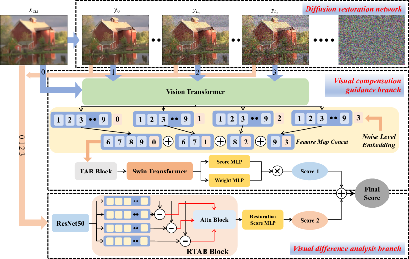
Figure 2: The illustration of proposed Diff$V^{2}$IQA. We begin by feeding the image into the diffusion restoration network, which produces the ultimate restored image along with two intermediate noise-containing images. Afterwards, all the images are input into two branches: the visual compensation guidance branch and the visual difference analysis branch. The former is built upon the vision transformer and integrates noise level embedding strategy to obtain a score, while the latter is based on ResNet50 and incorporates an attention mechanism to yield a score. The outcomes from both branches are amalgamated and analyzed to obtain the final quality score.

III Proposed Diffusion Model Based Visual Compensation Guidance and Visual Difference Analysis NR-IQA Method

Divided into four essential sub-sections, this chapter conducts a thorough examination of the overall architecture of our proposed model. The subsequent sections include three crucial components: the diffusion restoration network, visual compensation guidance branch, and visual difference analysis branch. Each sub-section intricately dissects the fundamental principles and functionalities of these components, offering a detailed comprehension of their roles within the overall framework.

III-A Overall Architecture

The overall framework of our model (see Fig. 2.) is primarily composed of three key components: the diffusion restoration network, the visual compensation guidance branch based on vision transformer (ViT) [48], and the visual difference analysis branch based on the residual attention module. Initially, the distorted image is input to the diffusion restoration network, generating one enhanced image and two noise-containing images. Following that, these resultant images, along with the original distorted image, are fed into the two visual evaluation branches, obtaining two respective scores, which are combined with designated weights to get the final quality score. In the visual compensation guidance branch, we use ViT for feature extraction, followed by the incorporation of noise level embedding strategy. Specific features are selected, spliced, and fused to capture both the original distorted image features and the high-level visual information introduced by the diffusion restoration network. Additionally, this process includes regularized information containing nonlinear noise. In the visual difference analysis branch, we initially employ ResNet50 for the preliminary encoding of visual features. Then all data is input into the RTAB for a holistic assessment of the differentiated information, ultimately yielding a score. In the following sections, we will provide a detailed exposition of the design principles and architectures underlying each branch module.

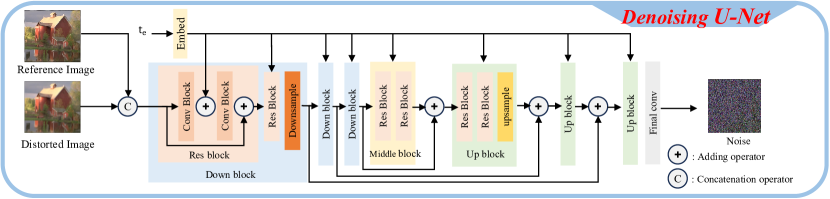
Figure 3: Overview of the pre-training process of the denoising model U-Net in our diffusion restoration network.

III-B Diffusion Restoration Network

III-B1 A Brief Introduction to Diffusion Model

Diffusion models belong to the class of likelihood-based models, and they leverage the U-Net architecture to reconstruct the distribution of training data. The U-Net is trained to eliminate noise from training data deliberately distorted by the addition of Gaussian noise. These models involve a forward noising process and a reverse denoising process. During the forward process, Gaussian noise is incrementally added to the original training data, denoted as $x_{0}\sim q(x_{o})$, in a step-by-step manner over T time steps, following a Markovian process:

$$q(x_{t}|x_{t-1})=\mathcal{N}(\sqrt{1-{\beta}_{t}}x_{t-1},{\beta}_{t}I)$$ (1)

where $\mathcal{N}(\cdot)$ is a Gaussian distribution, the Gaussian variances ${\beta}_{t=0}^{T}$ that determine the noise schedule can be learned or scheduled. Due to the preceding method, each timestep $t$ generates an arbitrary noisy sample $x_{t}$ directly from the initial sample $x_{0}$:

$$x_{t}=\sqrt{\bar{\alpha_{t}}}x_{0}+\sqrt{1-\bar{\alpha_{t}}}\epsilon,\epsilon\sim\mathcal{N}(0,I)$$ (2)

where $\alpha_{t}=1-\beta_{t}$, and $\bar{\alpha_{t}}=\prod_{s=1}^{T}\alpha_{s}$. In the reverse process, the diffusion model similarly adheres to a Markovian process to restore the noisy sample $x_{T}$ back to $x_{0}$. This denoising is performed step by step. In the case of large $T$ and small $\beta_{t}$, the reverse transition probability is approximated as a Gaussian distribution. This Gaussian distribution is predicted by a neural network that is trained to learn the reverse transitions, yielding the denoised sample $x_{0}$, which can be formulated as:

$$p_{\theta}(x_{t-1}|x_{t})=\mathcal{N}(x_{t-1};\mu_{\theta}(x_{t},t),\sigma_{\theta}(x_{t},t))$$ (3)

The re-parameterization of the reverse process involves estimating $\mu_{\theta}(x_{t},t)$ and $\sigma_{\theta}(x_{t},t)$. It is noteworthy that $\sigma_{\theta}(x_{t},t)$ is fixed at $\sigma_{t}^{2}I$, and the values of $\sigma_{t}^{2}I$ are not subject to learning. We then use U-Net to predict the one remaining item $\mu_{\theta}(x_{t},t)$, and the parameterization of $\mu_{\theta}(x_{t},t)$ is obtained as follows:

$$\mu_{\theta}(x_{t},t)=\frac{1}{\sqrt{\alpha_{t}}}(x_{t}-\frac{1-\alpha_{t}}{\sqrt{1-\bar{\alpha_{t}}}}\epsilon_{\theta}(x_{t},t))$$ (4)

The U-Net model, represented as $\epsilon_{\theta}(x_{t},t)$, is optimized by minimizing the following loss function:

$$\mathcal{L}(\theta)=E_{t,x_{0}.\epsilon}[(\epsilon-\epsilon_{\theta}(\sqrt{\bar{\alpha_{t}}}x_{0}+\sqrt{1-\bar{\alpha_{t}}\epsilon},t))^{2}]$$ (5)

Furthermore, when additional information is incorporated as conditional guidance for the network to converge, the final loss function is then formulated as :

$$\mathcal{L}(\theta)=E_{t,x_{0}.\epsilon}[(\epsilon-\epsilon_{\theta}(\sqrt{\bar{\alpha_{t}}}x_{0}+\sqrt{1-\bar{\alpha_{t}}\epsilon},t,x_{cond}))^{2}]$$ (6)

III-B2 The Architecture of Denoising Model U-Net

Algorithm 1 U-Net training process

1:  Repeat:

2:      $\epsilon\sim\mathcal{N}(0,I),\alpha\sim p(\alpha)$

3:      Take a gradient descent step on:    

$$\bigtriangledown_{\theta}(\epsilon-\epsilon_{\theta}(\sqrt{\bar{\alpha_{t}}}x_{dis}+\sqrt{1-\bar{\alpha_{t}}}\epsilon,t,x_{ref}))^{2}$$

4:  Until converged

Algorithm 2 Iterative image restoration process

1:  $y_{T}\sim\mathcal{N}(0,I)$

2:  for $t=T,...,1$ do:

3:      $z\sim\mathcal{N}(0,I)$ if $t>1$, else $z=0$

4:      $y_{t-1}=\frac{1}{\sqrt{\alpha_{t}}}(y_{t}-\frac{1-\alpha_{t}}{\sqrt{1-\gamma_{t}}}f_{\theta}(x_{dis},y_{t},\gamma_{t})+\sqrt{1-\alpha_{t}}z$

5:  end for

6:  return $y_{0},y_{t_{1}},y_{t_{2}}$ ($1<t_{1}.t_{2}<T$)

Our U-Net architecture is based on SR3 [46], a diffusion network designed for natural image super-resolution tasks (Fig. 3). Traditionally, in super-resolution tasks, networks learn a single type of distortion mapping by generating a low-resolution image through bicubic interpolation and pairing it with a high-resolution counterpart. However, in the IQA dataset, which contains various low-quality images, achieving generalized performance is challenging. To address this, we initially reduce the image chunk size, allowing for a significant increase in the batch size from 8 to 256. We also replace the original SR3 network’s GroupNorm, designed for a small batch size, with BatchNorm, better suited for the substantially increased batch size. Additionally, we remove specific preprocessing operations, such as bicubic upsampling before inputting the reference image into the SR3 network, driven by maintaining a consistent image size before and after this stage of processing.

These adjustments enhance the network’s ability to learn more generalized features, enabling it to execute image restoration tasks more effectively across a diverse set of images. Our approach aims to foster a broader understanding of image characteristics within the network, ultimately improving its overall performance and efficacy in image restoration tasks on the IQA dataset.

The training of the U-Net begins by feeding the distorted image into the network. This process involves using the reference image from the IQA dataset as conditional information, which is concatenated with the input image (Fig. 3). The network undergoes training until convergence following the steps outlined in Algorithm 1. In the image recovery process (Algorithm 2), at each time moment $t$, we continuously predict the noise, perform denoising and restoration operations, resulting in the enhanced image. Unlike SR3, our requirements extend beyond the final restored image; we also need intermediate variables representing the noise-containing restoration images at moments $t_{1}$ and $t_{2}$.

III-C Visual Compensation Guidance Branch

Through the diffusion restoration network, we obtain the final restored image along with intermediate noisy images ($y_{0},y_{t_{1}},y_{t_{2}}$). Then, we input these results into the ViT-based visual compensation guidance branch, simultaneously considering the original distorted image ($x_{dis}$). We structured our branch following the MANIQA [27] architecture. Similar to the approach outlined in that paper, we initially feed all the data into the ViT for preliminary extraction of feature information. The specific equation is shown below:

$$f_{dis}^{1},f_{dis}^{2}\dots f_{dis}^{9} =Net_{ViT}(x_{dis})$$ (7)

$$f_{0}^{1},f_{0}^{2}\dots f_{0}^{9} =Net_{ViT}(y_{0})$$

$$f_{1}^{1},f_{1}^{2}\dots f_{1}^{9} =Net_{ViT}(y_{t_{1}})$$

$$f_{2}^{1},f_{2}^{2}\dots f_{2}^{9} =Net_{ViT}(y_{t_{2}})$$

where $x_{dis}$ represents the input original image, $y_{0}$ signifies the ultimate recovered image produced by the diffusion model, while $y_{t_{1}}$ and $y_{t_{2}}$ denote the intermediate noise-containing images acquired during the denoising process of the diffusion model.

Following that, we choose partial feature maps for subsequent processing to mitigate excessive redundancy in feature information, which is in alignment with MANIQA. With the integration of the diffusion model, involving the restored image and the noise-containing images, we design a new reconstruction approach named noise level embedding strategy for obtaining new feature data map. We choose four feature maps from the original image obtained from ViT, followed by two feature maps from the final recovered image, and finally one feature map from each noise-containing image, which primarily utilizes the original image information and treat the diffusion introduced higher-level information as the visual compensation guidance In this process, inspired by the positional embedding principle in ViT, we propose a new noise level embedding strategy into the network to differentiate among the original image, the restored image, and the noise-containing images, as depicted in Fig. 2.

$$z_{dis} =[f_{dis}^{6},f_{dis}^{7},f_{dis}^{8},f_{dis}^{9}]+\textbf{{E}}_{NoiseCode}$$ (8)

$$z_{0} =[f_{0}^{6},f_{0}^{7}]+\textbf{{E}}_{NoiseCode}$$

$$z_{1} =[f_{1}^{8}]+\textbf{{E}}_{NoiseCode}$$

$$z_{2} =[f_{2}^{9}]+\textbf{{E}}_{NoiseCode}$$

For the original image, we opt to select a larger number of feature maps, with the expectation that the network can concentrate on crucial original distorted features. Simultaneously, we introduce additional high-level features and non-linear feature information as visual compensation guidance to aid in network learning. Following this, the four feature sets are concatenated to construct a new feature map, which is input into the posterior network for learning and training to ultimately obtain a quality score.

$$\textbf{{Z}}=Concatenate[z_{dis},z_{0},z_{1},z_{2}]$$ (9)

Upon acquiring the new feature map (Z), we traverse through the successive modules depicted in Fig. 2 to derive the ultimate score ($Score_{1}$) for the visual compensation guidance branch.

III-D Visual Difference Analysis Branch

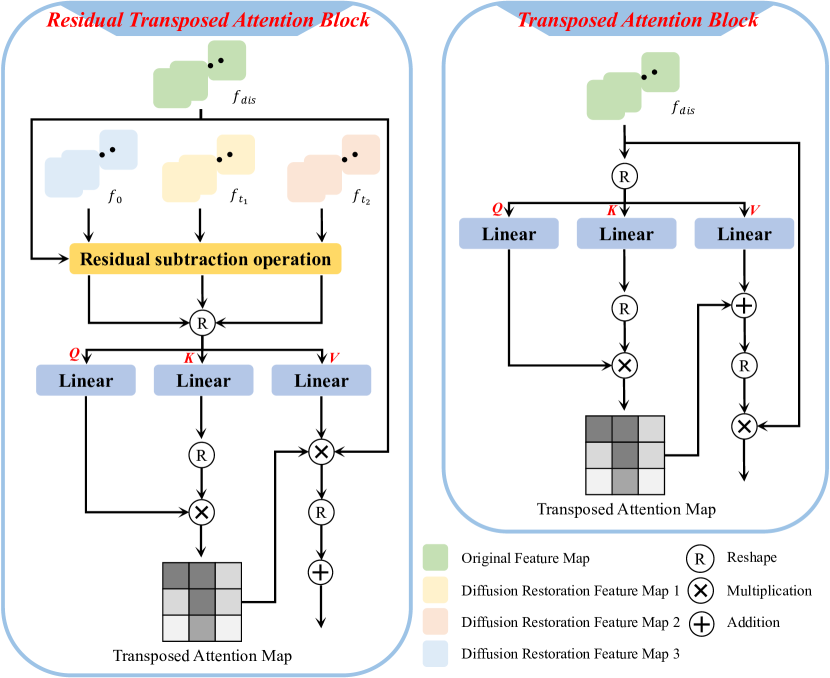
Figure 4: Comparison of our proposed Residual Transposed Attention Block with the Transposed Attention Block in the MANIQA paper and the specific architecture.

In order to fully exploit the high-level feature information introduced by the diffusion restoration network, we also devise a visual difference analysis branch specifically tailored for assessing the disparity information between the distorted and restored images. Firstly, we feed all the data into ResNet50 for feature extraction. Following that, the obtained results are input into the RTAB module. We opt not to persist with the transformer architecture for a specific reason: our emphasis in this context is solely on the difference information. The use of ViT could potentially introduce an excessive number of high-level feature variables, resulting in an overly complex model. Additionally, redirecting the data through ResNet into a completely new feature space is advantageous for enhancing the overall robustness of the model. We structured our RTAB drawing inspiration from the transposed attention block (TAB) in MANIQA, and a comparative analysis along with specific differences is illustrated in Fig. 4.

The TAB module incorporates a self-attention mechanism, utilizing itself as query (Q), key (K) and value (V) for posterior network learning. In our adaptation, we consolidate the original image, the restored image, and the noise-containing images, performing a subtraction operation before inputting them into the subsequent network as Q, K, and V for learning, respectively. The network learns by emphasizing information about the disparities between the original image and the restored and noisy images. It concentrates on evaluating the difference between the distorted image and restored images, ultimately producing a score. The specific equation is shown below:

$$\textbf{Q}:|x_{\text{dis}}-y_{0}|,\textbf{K}:|x_{\text{dis}}-y_{t_{1}}|,\textbf{V}:|x_{\text{dis}}-y_{t_{2}}|$$ (10)

$$\hat{\textbf{X}}=Attn(\textbf{{Q}, {K}, V})+\textbf{X}$$

$$Attn(\textbf{Q},\textbf{K},\textbf{V})=\textbf{V}\cdot Softmax(\frac{\textbf{K}\cdot\textbf{Q}}{\alpha})$$

Following RTAB, a restoration score MLP network was employed to ultimately obtain a score ($Score_{2}$) for the visual difference analysis branch. The final score of our model is expressed as follows, calculated through a weighted addition of the scores obtained from the two branches. The weight $\alpha$ is set to 0.3 in practice.

$$Score_{final}=Score_{1}+\alpha Score_{2}$$ (11)

IV Experiments

IV-A Experimental Settings

TABLE I: IQA Datasets used for training and evaluation.

Dataset	# Ref	# Dist	Dist Type	# Dist Type	Split	Original size $W\times H$	Train size (cropped patch)
LIVE[2]	29	779	Synthetic	5	8:2	768 × 512 (typical)	224 × 224
CISQ[49]	30	866	Synthetic	6	8:2	512 × 512	224 × 224
TID2013[50]	25	3000	Synthetic	24	8:2	512 × 384	224 × 224
KADID-10K[51]	81	10.1k	Synthetic	25	8:2	512 × 384	224 × 224
PIPAL[52]	250	29k	Syth.+alg.	116	Official	288 × 288	224 × 224
CLIVE[3]	-	1.2k	Authentic	-	8:2	500 × 500	224 × 224
KonIQ-10K[4]	-	10k	Authentic	-	8:2	512 × 384	224 × 224

IV-A1 Datasets

To ensure a rigorous and extensive evaluation of our proposed model’s performance, our principal investigation incorporated seven diverse datasets (see Table I). This ensemble consist of five synthetically distorted datasets: LIVE [2], CSIQ [49], TID2013 [50], Kadid10k [51] and PIPAL [52], complemented by two authentic distortion datasets: the LIVE Challenge (CLIVE) [3] and KonIQ10k [4]. Experiments addressing individual distortion types are carried out on the synthetic distortion datasets, specifically LIVE and CSIQ. Additionally, we conduct cross-dataset validation experiments using the LIVE, CSIQ, TID2013, PIPAL and CLIVE datasets. Finally, we investigate the pre-training datasets employed for our diffusion restoration network. We conduct comparative experiments to assess the impact of pre-training strategies based on the TID2013 and PIPAL datasets.

Consistent with established practices found in the majority of related research papers, we follow a standardized approach for processing datasets. Specifically, the training and testing datasets are randomly divided in an 8:2 ratio. During both training and testing phases, we employ random sampling of image blocks sized at $224\times 224$. This choice is motivated by our use of the pretrained ViT model for feature extraction, necessitating conformity in data dimensions. All reported results are obtained through 10 iterations of training and testing on the specific target dataset with randomly conducted splitting operations. The presented averages reflect the culmination of these results.

IV-A2 Evaluation Metrics

In our evaluation methodology, we incorporate two metrics that are extensively acknowledged for the assessment of model performance within the field. The first is Spearman’s rank order correlation coefficient (SRCC) and The second is Pearson’s linear correlation coefficient (PLCC). Both SRCC and PLCC are bounded within the interval [-1, 1], with values approaching 1 signifying superior performance.

IV-A3 Training Settings

Initially, our diffusion restoration network is pretrained on the PIPAL dataset, selected for its diverse range of distortion classes (116 categories). In our ablation studies (Table VIII, Fig. 5), we also conduct comparative analyses to evaluate the impact of different pre-training datasets. For the diffusion restoration network, we use the Adam algorithm for optimization, with a learning rate of 1e-5. The restoration process is accelerated using a cosine schedule, and 50 diffusion time steps are uniformly set for both training and testing. To capture more extensive image features, we increase the batch size to 256, necessitating a corresponding reduction in the crop size to $16\times 16$ pixels. For the optimization of our image IQA network, we employ the Adam optimizer with a learning rate and weight decay factor set at 1e-5. Training utilizes the Mean Squared Error (MSE) loss function. Given the simultaneous processing of multiple image types, including original, restored, and noise-perturbed images, the batch size is set to 4 to accommodate computational demands.

TABLE II: Comparison of Diff$V^{2}$IQA vs. SOTA NR-IQA Algorithms on Six Standard Datasets (Best Two Results Highlighted in Bold and Underlined). The Results Are Sourced from Original Papers Such as MANIQA, Re-IQA, etc. A ”-” Denotes Missing Results in the Original Papers.

	LIVE		CSIQ		TID2013		Kadid10k		CLIVE		KonIQ10k
Method	SRCC	PLCC	SRCC	PLCC	SRCC	PLCC	SRCC	PLCC	SRCC	PLCC	SRCC	PLCC
BRISQUE[9]	0.939	0.935	0.746	0.829	0.604	0.694	0.528	0.567	0.608	0.629	0.665	0.681
CORNIA[11]	0.947	0.950	0.678	0.776	0.678	0.768	0.516	0.558	0.629	0.671	0.780	0.795
DBCNN[16]	0.968	0.971	0.946	0.959	0.816	0.865	0.851	0.856	0.851	0.869	0.875	0.884
HyperIQA[17]	0.962	0.962	0.923	0.942	0.840	0.858	0.852	0.845	0.859	0.882	0.906	0.917
CONTRIQUE[29]	0.960	0.961	0.942	0.955	0.843	0.857	0.934	0.937	0.845	0.857	0.894	0.906
MUSIQ[25]	-	-	-	-	-	-	-	-	-	-	0.916	0.928
GraphIQA[24]	0.979	0.980	0.947	0.959	-	-	-	-	0.845	0.862	0.911	0.915
VCRNet[1]	0.973	0.974	0.943	0.955	0.846	0.875	-	-	0.856	0.865	0.894	0.909
CLIP-IQA[31]	-	-	-	-	-	-	-	-	-	-	0.895	0.909
LIQE[32]	0.970	0.951	0.936	0.939	-	-	0.930	0.931	0.904	0.910	0.919	0.908
Re-IQA[53]	0.971	0.972	0.944	0.964	0.804	0.861	0.872	0.885	0.840	0.854	0.914	0.923
DEIQT[54]	0.980	0.982	0.946	0.963	0.892	0.908	0.889	0.887	0.875	0.894	0.921	0.934
TReS[26]	0.969	0.968	0.942	0.922	0.863	0.883	0.859	0.858	0.846	0.877	0.915	0.928
MANIQA[27]	0.982	0.983	0.961	0.968	0.937	0.943	0.934	0.937	-	-	-	-
TOPIQ[42]	-	-	-	-	-	-	-	-	0.870	0.884	0.926	0.939
Diff$V^{2}$IQA	0.984	0.987	0.986	0.990	0.961	0.962	0.934	0.937	0.895	0.912	0.917	0.939

IV-B Experimental Results

IV-B1 Performance Evaluation on Individual Database

To evaluate the robustness and effectiveness of our proposed model, we conduct a comprehensive set of experiments involving six datasets—four synthetic distortion datasets and two authentic distortion datasets. We compare a total of 15 methodologies, including traditional approaches like BRISQUE [9] and CORNIA [11], as well as contemporary deep learning models. Among the deep learning-based contenders, we assess CNN-based architectures such as DBCNN [16] and HyperIQA [17], graph convolutional networks like GraphIQA [24], transformer-based models like MUSIQ [25], TReS [26], and MANIQA [27]. We also include a model based on contrastive learning, CONTRIQUE [29]. We carefully select representative models from each technological domain to ensure a thorough and balanced comparison.

Our training process strictly adheres to the experimental setups outlined in the source publications. Most reported results are directly sourced from the original papers, denoted by ‘-’. Throughout the training, we ensured consistency in random number seeds, varying only in network architectures to ensure a high level of experimental fairness. The results of these experiments are systematically documented in Table II.

In Table II, our newly developed Diff$V^{2}$IQA model consistently outperforms existing alternatives across all synthetic distortion datasets, including LIVE, CSIQ, TID2013, and Kadid10k, regardless of dataset size. Particularly noteworthy is the performance on the LIVE dataset, which is relatively straightforward. In this case, MANIQA shows commendable performance, making the improvements offered by our model somewhat modest. However, when dealing with the slightly more complex CSIQ and TID2013 datasets, our model’s advancements in metric performance are notably evident, achieving optimal scores of 0.986 and 0.990 on CSIQ, and 0.961 and 0.962 on TID2013, respectively.

However, despite achieving top-tier metrics, our model does not exhibit a similarly significant improvement when applied to authentic distortions within IQA datasets. The primary factor contributing to this observationour is that diffusion-based image restoration network is predominantly trained on various synthetic distortions, which may not sufficiently represent the intricacies of authentic distortions. The observed decrease in image quality scores in the presence of authentic distortions may be attributed to factors beyond pixel-level aberrations, such as high-level feature information, not effectively captured by the diffusion restoration network. This conjecture gains support from the fact that VCRNet, which similarly relies on the concept of image restoration based on synthetic distortions, also exhibits limited effectiveness in the face of authentic distortions. In summary, our proposed model showcases commendable performance on both synthetic and authentic distortion datasets. By incorporating high-level information through a diffusion restoration network, introducing non-linearity via noisy intermediate images, and subsequently employing a dual visual branch to discern the decoupling of diverse data types and establish a reconstructive link between distorted images and their respective quality scores, our approach achieves a high level of accuracy in quality assessment.

TABLE III: SRCC Results for Individual Distortion Types on the LIVE and CSIQ Databases (Best Two Results Highlighted in Bold and Underlined)

	LIVE					CSIQ
Method	JP2K	JPEG	WN	GBLUR	FF	JP2K	JPEG	WN	GBLUR	FN	CC
DIIVINE[8]	0.925	0.913	0.985	0.958	0.845	0.803	0.732	0.756	0.785	0.432	0.789
BRISQUE[9]	0.914	0.965	0.979	0.951	0.877	0.840	0.806	0.723	0.820	0.378	0.804
CORNIA[11]	0.936	0.934	0.962	0.926	0.912	0.831	0.513	0.664	0.836	0.493	0.462
HOSA[12]	0.928	0.936	0.964	0.964	0.934	0.818	0.733	0.604	0.841	0.500	0.716
DeepIQA[35]	0.968	0.953	0.979	0.970	0.897	0.934	0.922	0.944	0.901	0.867	0.847
TSCNN[37]	0.959	0.965	0.981	0.970	0.930	0.922	0.902	0.923	0.896	0.873	0.866
DBCNN[16]	0.963	0.976	0.982	0.971	0.918	0.946	0.951	0.947	0.939	0.943	0.883
HyperIQA[17]	0.949	0.961	0.982	0.926	0.936	0.960	0.934	0.927	0.915	0.931	0.874
RAN4IQA[22]	0.962	0.922	0.984	0.972	0.920	0.936	0.914	0.931	0.892	0.835	0.859
Hall-IQA[23]	0.969	0.975	0.992	0.973	0.953	0.924	0.933	0.942	0.901	0.842	0.861
GraphIQA [24]	0.979	0.978	0.978	0.978	0.979	0.947	0.947	0.948	0.947	0.948	0.947
VCRNet[1]	0.975	0.979	0.988	0.978	0.962	0.962	0.956	0.939	0.950	0.899	0.919
Diff$V^{2}$IQA	0.977	0.978	0.995	0.990	0.968	0.987	0.972	0.977	0.972	0.986	0.953

IV-B2 Performance Evaluation on Individual Distortion Types

To substantiate the efficacy of our model, we extend our experimental framework to include analyses of individual distortion types, the results of which are delineated in Table III. Our investigations predominantly focuse on the LIVE and CSIQ datasets. We draw comparisons across twelve methods. It is worth noting that the selection of methods compared during our individual distortion type experiments diverges from those included in earlier full dataset evaluations. This discrepancy arises due to the absence of individual distortion type experiment comparisons within the original publications of some previously examined methods, resulting in a lack of available comparative data.

Examination of the Table III reveals that our proposed Diff$V^{2}$IQA model attains superior performance on the LIVE dataset, securing the highest scores in all categories except for Fast Fading (FF), including JPEG2000 (JP2K), JPEG, White Noise (WN), and Gaussian Blur (GBLUR) distortions. In the case of the CSIQ dataset, our model consistently delivers the best results across all evaluated distortion categories. The aforementioned findings, in conjunction with prior experimental outcomes, mutually reinforce the conclusion that our model exhibits exceptional efficacy when applied to synthetically distorted datasets. This performance is largely attributable to the incorporation of high-level feature information facilitated by the diffusion restoration model, in synergy with the ViT model’s robust feature learning capabilities. The additional experiments focusing on singular distortion classes further substantiate the effectiveness of our proposed model.

IV-B3 Performance Evaluation Cross Different Databases

TABLE IV: SRCC Result of Cross Database Test (Best Two Results Highlighted in Bold and Underlined)

Training	TID2013			CLIVE
Testing	LIVE	CSIQ	CLIVE	LIVE	TID2013	CSIQ
BRISQUE[9]	0.724	0.568	0.109	0.244	0.275	0.236
CORNIA[11]	0.809	0.659	0.263	0.553	0.385	0.433
CNN[15]	0.532	0.598	0.104	0.103	0.021	0.095
DeepIQA[35]	0.805	0.683	0.009	0.323	0.141	0.323
DBCNN[16]	0.872	0.703	0.412	0.757	0.401	0.631
RAN4IQA[22]	0.811	0.694	0.036	0.296	0.157	0.276
VCRNet[1]	0.822	0.721	0.307	0.746	0.416	0.566
Diff$V^{2}$IQA	0.904	0.828	0.332	0.706	0.348	0.593

TABLE V: Evaluations on Cross Datasets. Each model is trained using PIPAL and subsequently tested on the LIVE and TID2013 datasets. The Comparative Experimental Results Are Sourced from MANIQA.

Training on		PIPAL
Testing on		LIVE		TID2013
		PLCC	SRCC	PLCC	SRCC
FR	PSNR	0.873	0.865	0.687	0.677
	WaDIQaM[35]	0.883	0.837	0.698	0.741
	RADN[55]	0.905	0.878	0.747	0.796
NR	TReS[26]	0.643	0.663	0.516	0.563
	MANIQA[27]	0.835	0.855	0.704	0.619
	Diff$V^{2}$IQA	0.765	0.806	0.727	0.649

To assess the generalization capability of the proposed Diff$V^{2}$IQA, we performed experiments in which the IQA database synthetically distorted was evaluated on the authentically distorted IQA database, and vice versa. The specific SRCC results are presented in Table IV. It is evident that all of our models consistently achieve top-2 metrics, even outperforming other models in several datasets. This substantiates the robust generalization ability of our proposed model. Additionally, given that the distortion types in synthetically and authentically distorted IQA databases are entirely different, it is challenging for IQA methods to generalize to authentically distorted databases when trained on synthetically distorted databases, and vice versa. In this scenario, our model continues to demonstrate excellent performance metrics, underscoring its robust generalization capabilities. While the diffusion restoration network of our model is trained on synthetic distortion, its effectiveness extends to a certain degree in handling authentic distorted images as well.

Furthermore, to further substantiate the generalization ability of our model, we performed additional experiments following the cross-dataset approach outlined in the MANIQA paper, as depicted in Table V. The training was conducted on the PIPAL dataset, and testing was carried out on TID2013 and the LIVE dataset. We conducted a comprehensive analysis by testing both SRCC and PLCC results. These were compared with several FR-IQA methods to thoroughly showcase the performance of our model. Notably, our model’s results on TID2013 stand out (PLCC: 0.727, SRCC: 0.649), even when compared to some full-reference methods. This further underscores the generalization performance of our model. In summary, the proposed Diff$V^{2}$IQA demonstrates robust generalization capabilities for both synthetic and authentic distortions.

IV-B4 Ablation Studies

TABLE VI: Ablation Study on Our Modules. Results Are Tested on TID2013 Dataset.

Diffusion	Noise embedding	RTAB	SRCC	PLCC
			0.937	0.943
✓			0.949	0.956
✓	✓		0.954	0.960
✓		✓	0.953	0.959
✓	✓	✓	0.961	0.962

TABLE VII: Ablation Study on Each Visual Evaluation Branch. Results Are Tested on TID2013 Dataset.

VCG Branch	VDA Branch	SRCC	PLCC
✓		0.942	0.950
	✓	0.909	0.912
✓	✓	0.961	0.962

On the individual components’ functionalities

In this section, we conducted experiments focusing on the individual components’ functionalities, as illustrated in Table VI. ‘Diffusion’ represents our diffusion restoration network, ‘Noise Embedding’ signifies the noise level embedding strategy, while ‘RTAB’ denotes the residual transposed attention block . We evaluated the results in terms of SRCC and PLCC on the TID2013 dataset. From Table VI, it can be observed that each component contributes significantly to the overall performance.

The diffusion restoration model adheres to the principle of iterative denoising, generating richer high-level visual information, such as the final repaired image and the noise-containing images from the intermediate process. These images offer more detailed, clearer, and richer information to guide the network in quality evaluation. The ‘Noise Embedding’ strategy, meticulously crafted for encoding noise levels in distinct image states, intricately refines the model’s capability to navigate diverse image conditions. This strategy empowers the network to discern to a certain extent between crucial original distorted image details and additional introduced high-level visual information, facilitating more effective learning of feature information.

Lastly, the RTAB dedicated to image restoration quality evaluation focuses on discerning the difference information between the original image and the restored image, including the noise-containing image. We conducted visualizations of selected images to offer a clearer representation of the similarities and differences between images at various quality levels after the diffusion restoration network, as illustrated in Fig. 5. Specifically, we selected three images with grades 1, 3, and 5 in the AWGN distortion type from the CSIQ dataset. The visualized difference maps for these images after the diffusion restoration network were compared with the original images. Upon observation of the results, notable improvements in image quality are apparent, particularly in images with higher noise levels. The corresponding error maps also reveal distinct variations among differently restored images. This disparity serves as a discernible indicator that the network successfully learns a crucial aspect: higher-quality images undergo more subtle changes during the restoration process, while lower-quality images exhibit more pronounced alterations. This observation underscores the network’s capability to adapt its restoration efforts based on the inherent quality of the input image.

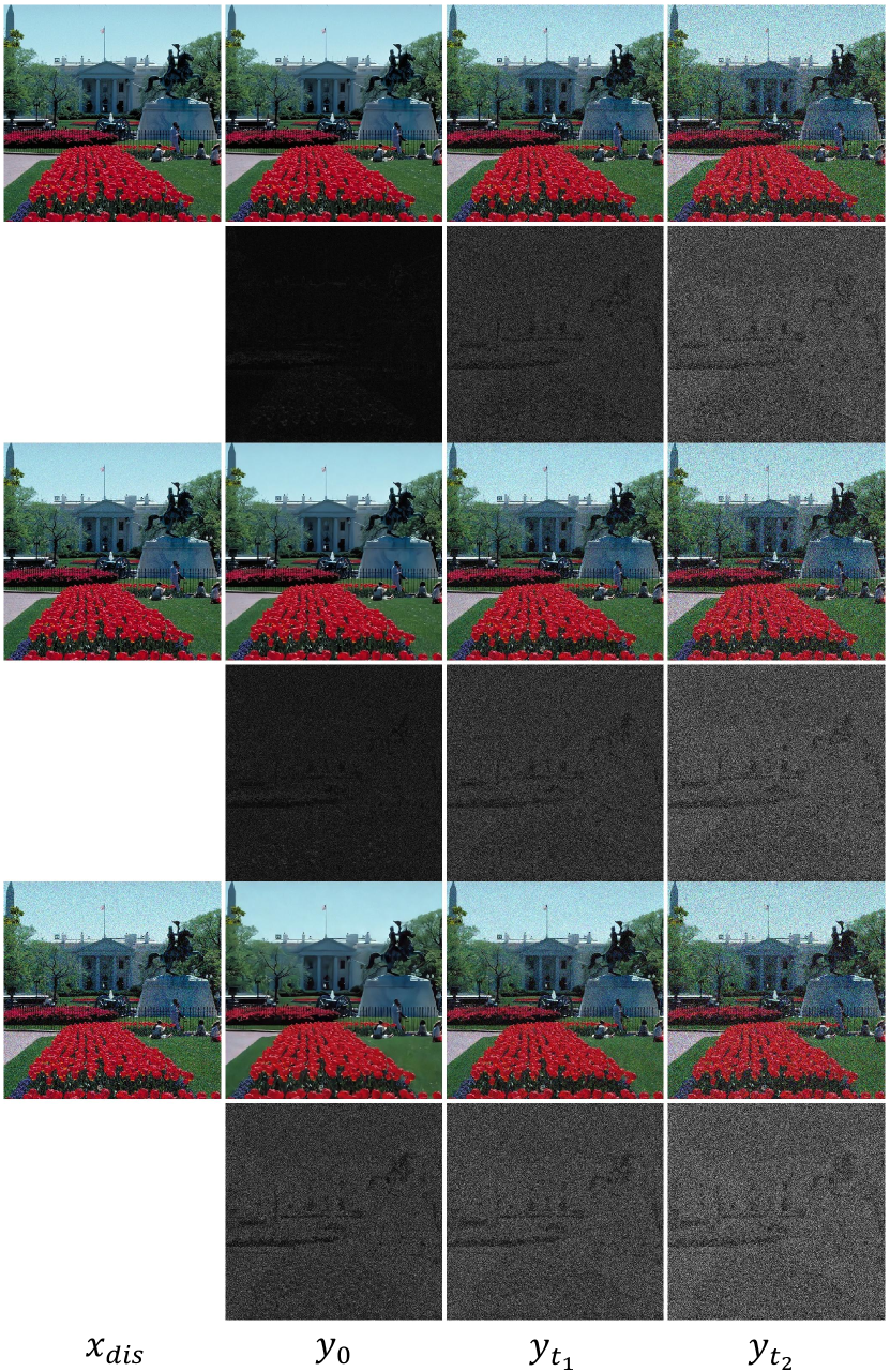
Figure 5: Visualization of the results from applying the diffusion model to the CSIQ dataset image “1600.AWGN.png”. The images selected for display correspond to noise levels 1, 3, and 5, arranged from top to bottom. In rows 1, 3, and 5, the last three columns respectively showcase the final diffusion model-generated images, images restored from the presence of first-level noise, and images restored from the presence of second-level noise. Rows 2, 4, and 6 feature the error maps resulting from the subtraction of each restored image from the original source image.

Overall, the combined effect of all components yields superior SRCC and PLCC values, underscoring the synergistic impact of these components on the overall performance of our proposed model. These findings validate the effectiveness of each module and highlight their collaborative role in achieving enhanced quality assessment results.

On the individual visual branch’ functionalities

We conducted ablation experiments for each functional branch, as detailed in Table VII, where VCG represents visual compensation guidance, and VDA represents visual difference analysis. Notably, optimal results were achieved when both branches were collaboratively engaged in quality evaluation. When the branches performed independent quality evaluation, it was observed that the VCG branch yielded superior results. This observation underscores the significance of the intrinsic features of the distorted image in quality assessment and further affirms the superiority of the transformer architecture over the ResNet architecture in capturing detailed features.

TABLE VIII: The Ablation Study of Pretrained Diffusion Model-Based Image Restoration Networks on Different Dataset, “Diff$V^{2}$IQA*” Denotes the Network Pre-trained on the TID2013 Dataset, While “Diff$V^{2}$IQA” Indicates Pre-training on the PIPAL Dataset.

	CSIQ		KonIQ10K		Kadid10K
	SRCC	PLCC	SRCC	PLCC	SRCC	PLCC
Diff$V^{2}$IQA*	0.985	0.989	0.909	0.926	0.926	0.930
Diff$V^{2}$IQA	0.986	0.990	0.917	0.939	0.934	0.937

On the variations in performance across different pre-training datasets for the diffusion model

We additionally performed extended experiments on diffusion restoration networks, specifically investigating the influence of the training effectiveness of the restoration networks on the overall performance of the model. We pre-trained our diffusion restoration network on two datasets: the TID2013 dataset and the PIPAL dataset. Each dataset utilized all available samples for training, with consistent parameters except for the dataset source. Following the initial training, we conducted quantitative experimental tests on three additional datasets, comprising two simulated distortion datasets and one real distortion dataset, as illustrated in Table VIII. The PIPAL dataset encompasses a more extensive training dataset (PIPAL: 23,200, TID2013: 3,000) and a greater variety of image distortion categories (PIPAL: 116, TID2013: 24) compared to the TID2013 dataset. Consequently, image restoration networks with enhanced generalization performance can be trained. From Table VIII, it is evident that when dealing with a dataset like CSIQ, which is not particularly complex, the difference in results between the two datasets is not significant. However, when faced with a larger synthetic distortion dataset or a authentic distortion dataset, the diffusion restoration network trained on PIPAL exhibits superior performance.

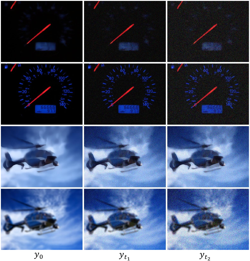
Figure 6: Visualization results of image restoration after pre-training on different datasets. Rows 1 and 3 illustrate models pre-trained on the TID2013 dataset, while rows 2 and 4 display models pre-trained on the PIPAL dataset. The images are sourced respectively from the KonIQ and Kadid datasets.

Additionally, we conducted visualizations of repaired images along with noise-containing images acquired under different pre-training datasets, as depicted in Fig. 6. It is evident that the enhanced images obtained through training on the larger and more diverse PIPAL dataset are clearer and align more closely with the standard of high-quality images. In contrast, under TID2013 training, the network faces challenges in recovering and enhancing certain detailed texture information. In conclusion, the selection of the pre-training dataset significantly impacts the performance of our model, with the PIPAL dataset yielding superior results.

On the weight proportions of the two branches

Our image quality evaluation stage is bifurcated into two branches, and we have conducted experiments to discuss and validate the impact of the weight assigned to the merged sum of the last two branches, as illustrated in Table IX. We systematically vary the weight assigned to the image restoration network branch from 0.1 to 1.5 in incremental steps. This adjustment is aimed at directing the network’s focus, emphasizing the importance of original image information and gradually shifting towards the image restoration difference information.

TABLE IX: Ablation Study of Different Scale Factors of the Image Restoration Score Branch on TID2013 Dataset. The Best Score is the Sum of SRCC and PLCC.

Scale	SRCC	PLCC	Best Score
0.1	0.9596	0.9620	1.9216
0.3	0.9612	0.9641	1.9253
0.6	0.9592	0.9632	1.9224
1	0.9602	0.9651	1.9253
1.5	0.9603	0.9642	1.9245

We observe that setting the weight near 0.3 optimizes the overall performance metrics of the model. This highlights that, in the context of quality evaluation, the foundational criterion for judging image quality remains rooted in the intrinsic quality of the image itself. Overemphasizing the restoration of enhanced images may lead to the oversight of crucial features in the original image. The information from the enhanced image serves as valuable supplementary data to aid the network in making judgments but should not be overly relied upon.

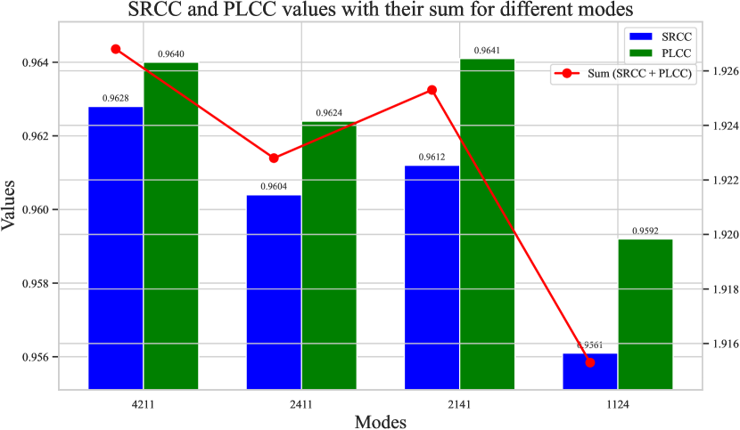
Figure 7: Ablation experiment regarding data input under various modality settings on the TID2013 dataset. For instance, the notation ‘4211’ signifies the selection of four data blocks processed by the ViT with original data, two blocks restored using the diffusion model, and one block each from noise levels 1 and 2.

On the context of employing different ratio schemes for original, augmented, and noisy images

We conducted noise level embedding in the ViT-based assessment branch for the original image, the enhanced image, and the noise-containing images. Subsequently, feature information of varying lengths from different images was selected for feature splicing, facilitating network feature recognition. To validate the rationality of our chosen ratio, we designed experiments, as illustrated in Fig. 7. We selected a total of 8 feature maps for feature splicing. The notation ‘4211’ in the figure signifies that 4, 2, 1, and 1 blocks of feature maps were chosen for splicing in the original image, the enhanced image, the image with noise level 1, and the image with noise level 2, respectively.

As observed in Fig. 7, similar to the earlier experimental findings, consistent conclusions emerge: a greater emphasis on the feature information of the original image is necessary. Overemphasizing the additional information introduced by the image enhancement network can prove detrimental to the network’s learning process. In summary, our selection of feature maps is both rational and effective, enabling the network to more effectively extract data feature information and yield superior results.

V Conclusion

Contribution: In this paper, we propose a new Diff$V^{2}$IQA model specifically designed for NR-IQA tasks. Notably, we pioneer the incorporation of the diffusion model into the NR-IQA domain. Followed free energy principle, we have innovatively designed a novel diffusion restoration network with heightened capability in capturing specific and intricate features. Furthermore, to comprehensively analyze the extracted high-level visual information, we devised two distinct visual evaluation branches. The first is a visual compensation guidance branch built on the transformer architecture, integrating a noise embedding strategy. The second involves a visual difference analysis branch rooted in the ResNet architecture and we proposed RTAB to better catch the detailed difference between distorted and restored images. These two branches assess quality from distinct perspectives and ultimately converge their analyses to derive the overall quality score. Extensive experiments substantiate the effectiveness of our model, showcasing its superiority over SOTA methods in recent years. Rigorous experimentation on various aspects of our network design and the selection of hyperparameters further attests to the rationality and effectiveness of our proposed approach. In conclusion, our Diff$V^{2}$IQA model emerges as highly effective, achieving SOTA performance in the domain of NR-IQA.

Limitation and Future Work: Firstly, the model must undergo pre-training of the diffusion restoration network, a process that is not as succinct as certain end-to-end direct quality evaluation networks. Furthermore, the diffusion restoration network exhibits a certain degree of dependence on the pre-trained dataset. Additionally, owing to the iterative denoising principle inherent in the diffusion model, there is an inherent extension of inference time to some extent. In our future work, we will concentrate on alleviating this issue and intend to progressively transition our research towards more advanced aspects of video tasks.

References

- [1] Z. Pan, F. Yuan, J. Lei, Y. Fang, X. Shao, and S. Kwong, “Vcrnet: Visual compensation restoration network for no-reference image quality assessment,” IEEE Trans. Image Process., vol. 31, pp. 1613–1627, Jan. 2022.
- [2] H. R. Sheikh, M. F. Sabir, and A. C. Bovik, “A statistical evaluation of recent full reference image quality assessment algorithms,” IEEE Trans. Image Process., vol. 15, no. 11, pp. 3440–3451, Oct. 2006.
- [3] D. Ghadiyaram and A. C. Bovik, “Massive online crowdsourced study of subjective and objective picture quality,” IEEE Trans. Image Process., vol. 25, no. 1, pp. 372–387, Nov. 2015.
- [4] V. Hosu, H. Lin, T. Sziranyi, and D. Saupe, “Koniq-10k: An ecologically valid database for deep learning of blind image quality assessment,” IEEE Trans. Image Process., vol. 29, pp. 4041–4056, Jan. 2020.
- [5] Y. Fang, J. Yan, L. Li, J. Wu, and W. Lin, “No reference quality assessment for screen content images with both local and global feature representation,” IEEE Trans. Image Process., vol. 27, no. 4, pp. 1600–1610, Dec. 2017.
- [6] Y. Fang, K. Ma, Z. Wang, W. Lin, Z. Fang, and G. Zhai, “No-reference quality assessment of contrast-distorted images based on natural scene statistics,” IEEE Signal Process. Letters, vol. 22, no. 7, pp. 838–842, Nov. 2014.
- [7] Q. Li, W. Lin, J. Xu, and Y. Fang, “Blind image quality assessment using statistical structural and luminance features,” IEEE Trans. Multimedia, vol. 18, no. 12, pp. 2457–2469, Aug. 2016.
- [8] A. K. Moorthy and A. C. Bovik, “Blind image quality assessment: From natural scene statistics to perceptual quality,” IEEE Trans. Image Process., vol. 20, no. 12, pp. 3350–3364, Apr. 2011.
- [9] A. Mittal, A. K. Moorthy, and A. C. Bovik, “No-reference image quality assessment in the spatial domain,” IEEE Trans. Image Process., vol. 21, no. 12, pp. 4695–4708, Aug. 2012.
- [10] C. Li, A. C. Bovik, and X. Wu, “Blind image quality assessment using a general regression neural network,” IEEE Trans. Neural Netw., vol. 22, no. 5, pp. 793–799, Apr. 2011.
- [11] P. Ye, J. Kumar, L. Kang, and D. Doermann, “Unsupervised feature learning framework for no-reference image quality assessment,” in 2012 IEEE Conf. Comput. Vis. Pattern Recognit. (CVPR), Jun. 2012, pp. 1098–1105.
- [12] J. Xu, P. Ye, Q. Li, H. Du, Y. Liu, and D. Doermann, “Blind image quality assessment based on high order statistics aggregation,” IEEE Trans. Image Process., vol. 25, no. 9, pp. 4444–4457, Jun. 2016.
- [13] L. Xu, J. Li, W. Lin, Y. Zhang, L. Ma, Y. Fang, and Y. Yan, “Multi-task rank learning for image quality assessment,” IEEE Trans. Circuits Syst. Video Technol., vol. 27, no. 9, pp. 1833–1843, Mar. 2016.
- [14] K. Gu, D. Tao, J.-F. Qiao, and W. Lin, “Learning a no-reference quality assessment model of enhanced images with big data,” IEEE Trans. Neural Netw. Trans. Neural Netw. Syst., vol. 29, no. 4, pp. 1301–1313, Mar. 2017.
- [15] L. Kang, P. Ye, Y. Li, and D. Doermann, “Convolutional neural networks for no-reference image quality assessment,” in Proc. IEEE Conf. Comput. Vis. Pattern Recognit. (CVPR), Jan. 2014, pp. 1733–1740.
- [16] W. Zhang, K. Ma, J. Yan, D. Deng, and Z. Wang, “Blind image quality assessment using a deep bilinear convolutional neural network,” IEEE Trans. Circuits Syst. Video Technol., vol. 30, no. 1, pp. 36–47, Jan. 2018.
- [17] S. Su, Q. Yan, Y. Zhu, C. Zhang, X. Ge, J. Sun, and Y. Zhang, “Blindly assess image quality in the wild guided by a self-adaptive hyper network,” in Proc. IEEE/CVF Conf. Comput. Vis. Pattern Recognit. (CVPR), Jan. 2020, pp. 3667–3676.
- [18] H. Chen, X. Chai, F. Shao, X. Wang, Q. Jiang, M. Chao, and Y.-S. Ho, “Perceptual quality assessment of cartoon images,” IEEE Trans. Multimedia, vol. 25, pp. 140–153, Oct. 2021.
- [19] W. Zhou, J. Xu, Q. Jiang, and Z. Chen, “No-reference quality assessment for 360-degree images by analysis of multifrequency information and local-global naturalness,” IEEE Trans. Circuits Syst. Video Technol., vol. 32, no. 4, pp. 1778–1791, May. 2021.
- [20] J. Xu, W. Zhou, H. Li, F. Li, and Q. Jiang, “Quality assessment of multi-exposure image fusion by synthesizing local and global intermediate references,” Displays, vol. 74, p. 102188, Sep. 2022.
- [21] Q. Jiang, F. Shao, W. Lin, K. Gu, G. Jiang, and H. Sun, “Optimizing multistage discriminative dictionaries for blind image quality assessment,” IEEE Trans. Multimedia, vol. 20, no. 8, pp. 2035–2048, Oct. 2017.
- [22] H. Ren, D. Chen, and Y. Wang, “Ran4iqa: Restorative adversarial nets for no-reference image quality assessment,” in Proc. AAAI Conf. artificial Intell., vol. 32, no. 1, Aug. 2018.
- [23] K.-Y. Lin and G. Wang, “Hallucinated-iqa: No-reference image quality assessment via adversarial trans. neural netw.ing,” in Proc. IEEE Conf. Comput. Vis. Pattern Recognit. (CVPR), Apr. 2018, pp. 732–741.
- [24] S. Sun, T. Yu, J. Xu, W. Zhou, and Z. Chen, “Graphiqa: Learning distortion graph representations for blind image quality assessment,” IEEE Trans. Multimedia, Jan 2022.
- [25] J. Ke, Q. Wang, Y. Wang, P. Milanfar, and F. Yang, “Musiq: Multi-scale image quality transformer,” in Proc. IEEE/CVF International Conf. Comput. Vis. (ICCV), Aug. 2021, pp. 5148–5157.
- [26] S. A. Golestaneh, S. Dadsetan, and K. M. Kitani, “No-reference image quality assessment via transformers, relative ranking, and self-consistency,” in Proc. IEEE/CVF Winter Conf. Applications of Comput. Vis., Jan. 2022, pp. 1220–1230.
- [27] S. Yang, T. Wu, S. Shi, S. Lao, Y. Gong, M. Cao, J. Wang, and Y. Yang, “Maniqa: Multi-dimension attention network for no-reference image quality assessment,” in Proc. IEEE/CVF Conf. Comput. Vis. Pattern Recognit. (CVPR), Apr. 2022, pp. 1191–1200.
- [28] K. Zhao, K. Yuan, M. Sun, M. Li, and X. Wen, “Quality-aware pre-trained models for blind image quality assessment,” Mar. 2023.
- [29] P. C. Madhusudana, N. Birkbeck, Y. Wang, B. Adsumilli, and A. C. Bovik, “Image quality assessment using contrastive learning,” IEEE Trans. Image Process., vol. 31, pp. 4149–4161, Jun. 2022.
- [30] S. Roy, S. Mitra, S. Biswas, and R. Soundararajan, “Test time adaptation for blind image quality assessment,” in Proc. IEEE/CVF Int. Conf. Comput. Vis. (ICCV), Aug. 2023, pp. 16 742–16 751.
- [31] J. Wang, K. C. Chan, and C. C. Loy, “Exploring clip for assessing the look and feel of images,” in Proc. AAAI Conf. Artificial Intell., vol. 37, no. 2, Jun. 2023, pp. 2555–2563.
- [32] W. Zhang, G. Zhai, Y. Wei, X. Yang, and K. Ma, “Blind image quality assessment via vision-language correspondence: A multitask learning perspective,” in Proc. IEEE/CVF Conf. Comput. Vis. and Pattern Recognit. (CVPR), Jan. 2023, pp. 14 071–14 081.
- [33] Ž. Babnik, P. Peer, and V. Štruc, “Diffiqa: Face image quality assessment using denoising diffusion probabilistic models,” arXiv preprint arXiv:2305.05768, May. 2023.
- [34] J. Kim, H. Zeng, D. Ghadiyaram, S. Lee, L. Zhang, and A. C. Bovik, “Deep convolutional neural models for picture-quality prediction: Challenges and solutions to data-driven image quality assessment,” IEEE Signal Process. Mag., vol. 34, no. 6, pp. 130–141, Nov. 2017.
- [35] S. Bosse, D. Maniry, K.-R. Müller, T. Wiegand, and W. Samek, “Deep neural networks for no-reference and full-reference image quality assessment,” IEEE Trans. Image Process., vol. 27, no. 1, pp. 206–219, Oct. 2017.
- [36] S. Bianco, L. Celona, P. Napoletano, and R. Schettini, “On the use of deep learning for blind image quality assessment,” Signal, Image and Video Process., vol. 12, pp. 355–362, Aug. 2018.
- [37] Q. Yan, D. Gong, and Y. Zhang, “Two-stream convolutional networks for blind image quality assessment,” IEEE Trans. Image Process., vol. 28, no. 5, pp. 2200–2211, Nov. 2018.
- [38] L.-M. Po, M. Liu, W. Y. Yuen, Y. Li, X. Xu, C. Zhou, P. H. Wong, K. W. Lau, and H.-T. Luk, “A novel patch variance biased convolutional neural network for no-reference image quality assessment,” IEEE Trans. Circuits Syst. Video Technol., vol. 29, no. 4, pp. 1223–1229, Jan. 2019.
- [39] X. Liu, J. Van De Weijer, and A. D. Bagdanov, “Rankiqa: Learning from rankings for no-reference image quality assessment,” in Proc. IEEE Int. Conf. Comput. Vis. (ICCV), Jul. 2017, pp. 1040–1049.
- [40] K. Ma, W. Liu, K. Zhang, Z. Duanmu, Z. Wang, and W. Zuo, “End-to-end blind image quality assessment using deep neural networks,” IEEE Trans. Image Process., vol. 27, no. 3, pp. 1202–1213, Nov. 2017.
- [41] X. Chen, H. Fan, R. Girshick, and K. He, “Improved baselines with momentum contrastive learning,” arXiv preprint arXiv:2003.04297, Mar. 2020.
- [42] C. Chen, J. Mo, J. Hou, H. Wu, L. Liao, W. Sun, Q. Yan, and W. Lin, “Topiq: A top-down approach from semantics to distortions for image quality assessment,” arXiv preprint arXiv:2308.03060, Aug. 2023.
- [43] J. Ho, A. Jain, and P. Abbeel, “Denoising diffusion probabilistic models,” in Advances in Neural Information Process. Syst., H. Larochelle, M. Ranzato, R. Hadsell, M. Balcan, and H. Lin, Eds., vol. 33. Curran Associates, Inc., 2020, pp. 6840–6851. [Online]. Available: https://proceedings.neurips.cc/paper_files/paper/2020/file/4c5bcfec8584af0d967f1ab10179ca4b-Paper.pdf
- [44] A. Q. Nichol and P. Dhariwal, “Improved denoising diffusion probabilistic models,” in Proc. 38th International Conf. Machine Learning, ser. Proceedings of Machine Learning Research, M. Meila and T. Zhang, Eds., vol. 139. PMLR, 18–24 Jul Apr. 2021, pp. 8162–8171. [Online]. Available: https://proceedings.mlr.press/v139/nichol21a.html
- [45] H. Li, Y. Yang, M. Chang, S. Chen, H. Feng, Z. Xu, Q. Li, and Y. Chen, “Srdiff: Single image super-resolution with diffusion probabilistic models,” Neurocomputing, vol. 479, pp. 47–59, Mar. 2022.
- [46] C. Saharia, J. Ho, W. Chan, T. Salimans, D. J. Fleet, and M. Norouzi, “Image super-resolution via iterative refinement,” IEEE Trans. Pattern Anal. Mach. Intell., vol. 45, no. 4, pp. 4713–4726, Sep. 2022.
- [47] R. Rombach, A. Blattmann, D. Lorenz, P. Esser, and B. Ommer, “High-resolution image synthesis with latent diffusion models,” in Proc. IEEE/CVF Conf. Comput. Vis. Pattern Recognit. (CVPR), Apr. 2022, pp. 10 684–10 695.
- [48] A. Dosovitskiy, L. Beyer, A. Kolesnikov, D. Weissenborn, X. Zhai, T. Unterthiner, M. Dehghani, M. Minderer, G. Heigold, S. Gelly et al., “An image is worth 16x16 words: Transformers for image recognition at scale,” arXiv preprint arXiv:2010.11929, Jun. 2020.
- [49] E. C. Larson and D. M. Chandler, “Most apparent distortion: full-reference image quality assessment and the role of strategy,” Journal of electronic imaging, vol. 19, no. 1, pp. 011 006–011 006, Jan. 2010.
- [50] N. Ponomarenko, L. Jin, O. Ieremeiev, V. Lukin, K. Egiazarian, J. Astola, B. Vozel, K. Chehdi, M. Carli, F. Battisti et al., “Image database tid2013: Peculiarities, results and perspectives,” Signal Process.: Image Commun., vol. 30, pp. 57–77, Jan. 2015.
- [51] H. Lin, V. Hosu, and D. Saupe, “Kadid-10k: A large-scale artificially distorted iqa database,” in 2019 Eleventh International Conference on Quality of Multimedia Experience (QoMEX). IEEE, Jun. 2019, pp. 1–3.
- [52] J. Gu, H. Cai, H. Chen, X. Ye, J. Ren, and C. Dong, “Image quality assessment for perceptual image restoration: A new dataset, benchmark and metric,” arXiv preprint arXiv:2011.15002, Nov. 2020.
- [53] A. Saha, S. Mishra, and A. C. Bovik, “Re-iqa: Unsupervised learning for image quality assessment in the wild,” in Proc. IEEE/CVF Conf. Comput. Vis. Pattern Recognit. (CVPR), Jan. 2023, pp. 5846–5855.
- [54] G. Qin, R. Hu, Y. Liu, X. Zheng, H. Liu, X. Li, and Y. Zhang, “Data-efficient image quality assessment with attention-panel decoder,” arXiv preprint arXiv:2304.04952, Apr. 2023.
- [55] S. Shi, Q. Bai, M. Cao, W. Xia, J. Wang, Y. Chen, and Y. Yang, “Region-adaptive deformable network for image quality assessment,” in Proc. IEEE/CVF Conf. Comput. Vis. Pattern Recognit. (CVPR), Apr. 2021, pp. 324–333.