Modeling 3D Infant Kinetics Using Adaptive Graph Convolutional Networks

Abstract

Reliable methods for the neurodevelopmental assessment of infants are essential for early detection of medical issues that may need prompt interventions. Spontaneous motor activity, or ‘kinetics’, is shown to provide a powerful surrogate measure of upcoming neurodevelopment. However, its assessment is by and large qualitative and subjective, focusing on visually identified, age-specific gestures. Here, we follow an alternative approach, predicting infants’ neurodevelopmental maturation based on data-driven evaluation of individual motor patterns. We utilize 3D video recordings of infants processed with pose-estimation to extract spatio-temporal series of anatomical landmarks, and apply adaptive graph convolutional networks to predict the actual age. We show that our data-driven approach achieves improvement over traditional machine learning baselines based on manually engineered features.

1 Introduction

Early identification of neurodevelopmental issues is essential for supporting lifelong neurocognitive performance. A frequent neurodevelopmental follow-up is routine practice for the over 10 percent of infants who are identified to be at developmental risk based on their pre- or postnatal medical adversities [20] such as prematurity, birth asphyxia, stroke or metabolic disorders. Early start of interventions is crucial to minimize the long-term impacts on individuals and societies. However, it remains challenging to identify these infants efficiently, objectively and at scale [18].

It is now well established that infants’ spontaneous movements provide a sensitive tool for predicting problems in later neurodevelopment. In both routine and research contexts, spontaneous movements are commonly assessed by trained experts who use the General Movements Assessment (GMA) paradigm [6]. It was originally developed to visually recognize a few age-specific movement patters. In the current clinical practise, the GMA paradigm is typically used to predict later development of cerebral palsy by observing infants’ expression of discrete gestures called ‘fidgety movements’ at about 3 months of age [10]. As the GMA paradigm needs visual inspection by well trained experts, several algorithmic approaches have been developed to emulate visual assessment based on movement- and/or video recordings [1, 25, 19, 27]. These models are reported to perform reasonably well; however, their performance is challenged by a strong class imbalance, namely, the scarcity of training targets for fidgety movements. Moreover, a significant amount of each video frame contain information unrelated to the target patterns, e.g. background or illumination, which reduces signal-to-noise ratio dramatically. Therefore, recent studies have explored a variety of machine learning methods using 2D pose estimated data to perform classifications related to abnormality [3, 15, 21, 17, 12].

Here, we aim for an alternative approach: instead of emulating experts’ video evaluation, we choose to target age prediction. It is motivated by the ubiquitous pediatric practice that age is used as the key benchmark for evaluating a child’s status; that is, determining whether a child is developing typically for their age or exhibiting neurodevelopmental delay. Therefore, an age prediction algorithm from kinetics in typically developing infants should provide a maximally generalizable, explainable, and transparent proxy of infants’ neurodevelopmental maturity [26]. The proposed method extends previous work where linear regression was applied on limb movement parameters for determining age [13]. We compile a novel 3D video dataset from infants’ neurodevelopmental assessments in two research centers, and incorporate spatio-temporal information in the modeling using Adaptive Graph Convolutional Networks (AAGCNs) [23]. The model offers notable strengths: it is tailored for skeletal data and includes learnable adjacency matrices and attention mechanisms for each individual input sample. Through our experiments, we demonstrate that: 1) the data-driven approach offers performance improvements over using hand-crafted limb features, 2) poses obtained in 3D are advantageous compared to the more broadly studied 2D data, and 3) the model provides prediction explainability with potential applications in medical and research contexts.

2 Dataset

2.0.1 Infant Recordings.

The data used in this study was collated from larger research trials in Pisa and Helsinki. The ethical approval was provided for the Italian cohort by Tuscany Paediatrics Ethics Committee (nr. 187/2020) and for the Finnish cohort, the study protocol was approved by the Institutional Research Review Board at Helsinki University Hospital Medical Imaging Centre. In both countries, written informed consent was obtained from the parents/legal guardians in accordance with the Declaration of Helsinki. We used 3D video cameras with a tablet-based operating software (Neuro Event Labs Ltd) to record spontaneous movements of infants. The overall setup followed the established protocol by the GMs Trust [5]. During these sessions, the infants were placed supine, and care was taken to ensure that the recordings were made during periods of active wakefulness while minimizing environmental interferences. Skeletal videos were produced using a computational pose estimation model, and time series of (x, y, z)-coordinates from 18 anatomical landmarks were extracted [14]. The two datasets from two separate institutes could be combined to one larger cohort because they were based on identical video recording device and the same pose estimation pipeline.

2.0.2 Subject Selection and Video Segmentation.

We include 180 recorded infants for analysis, with corrected postnatal ages ranging from 27 to 158 days (average: 91 days, standard deviation: 22 days). This age range covers a period in early development where infants demonstrate notable changes in their motor development. The data preparation involves extracting segments of high quality from the recordings based on expert annotations, where periods of crying, fussiness, or other forms of distress are filtered out. To accommodate the input shapes spatio-temporal neural networks operate on, the video segments are standardized to a length of 600 timesteps, equivalent to 20 seconds, which resulted in a dataset 1890 samples large. Segments shorter than 600 timesteps are repeated if necessary to meet the length requirement. Baseline machine learning techniques explored in this work are based directly on data from the annotated segments.

2.0.3 Rotation Strategy.

Following the partitioning, we aim to standardize the videos so that they are as invariant as possible to the filming angle. For each video frame, the neck joint’s coordinates are subtracted from all other joints to establish a relative positioning. Subsequently, we apply a series of rotational transformations around the principal axes on the skeletal data extracted from pose-estimated videos to ensure a consistent orientation across video samples. Following the coordinate system shown in Fig. 1, the average spine vector from the neck to the center of the hip is aligned with the $y$-axis by rotating around the $z$-axis. The average spine is then made parallel with the $y$-axis by rotating around the $x$-axis. Lastly, the backline, calculated as an average of the hipline and the shoulderline, is aligned with the $x$-axis by rotating around the $y$-axis.

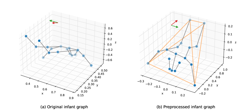
Figure 1: Preprocessing strategy of infant graphs. The average original graph of one recorded segment is shown to the left, with the direction of the spine vector in red, and the backline vector (average of hipline and shoulderline) in green. The resulting graph after preprocessing is displayed to the right, with newly introduced bidirectional edges.

2.0.4 Graph Construction.

In our proposed model, the human skeleton is represented as a graph, $\mathcal{G}=(\mathcal{V},\mathcal{E})$, where $\mathcal{V}$ is the set of vertices corresponding to the human joints, and $\mathcal{E}$ is the set of edges defining the physical connections between these joints. We consider 18 nodes representing the main joints extracted by pose estimation in the human body, as depicted by blue markers in Fig. 1. The physical structure of the human body is represented by 17 directed edges (gray lines), which follows the inherent skeletal connectivity of humans. Additionally, we introduce 6 bidirectional edges between the hands and feet, visualized as orange dotted lines. These edges are created to capture the coordinated movements between hands and feet, which often are of interest when studying infant development. Consecutive graphs in the recordings are connected temporally so that each joint at a given time step is connected to its corresponding joint in the adjacent time steps. The final spatio-temporal graph construction allows us to simultaneously model spatial relationships between different body parts at a given time, and their temporal evolution.

3 Method

3.0.1 Problem Formulation.

Given a sequence of infant skeleton recordings, we formulate the machine learning problem as the task to predict the age of the infant. Each recording is represented as a spatio-temporal graph, where nodes correspond to skeletal joints, and edges represent the physical connections between these joints. Let $\mathbf{X}\in\mathbb{R}^{C\times T\times V}$ be the input tensor, where $C=3$ represents spatial coordinates as node features, $T=600$ is the temporal dimension, and $V=18$, is the number of vertices, or joints in the infant graphs.

3.0.2 Graph Partitioning.

Spatio-temporal Graph Convolutional Networks (ST-GCN) [28] introduces a novel spatial configuration partitioning strategy that capitalizes on the inherent spatial locality of the human skeleton. The strategy divides the neighbor set of each node into three distinct subsets:

1. The root node itself.

2. The centripetal group: neighboring nodes that are closer to the skeleton’s gravity center than the root node.

3. The centrifugal group: nodes that are farther from the gravity center compared to the root node.

The gravity center at each frame is computed as the average coordinate of all joints. This partitioning reflects natural concentric and eccentric motions.

3.0.3 Spatio-Temporal Graph Convolutional Block.

STGCN operates on the graph by applying spatial and temporal convolutions. The spatial graph convolution can be formulated as:

$$\textbf{X}_{\mathit{out}}=\sum_{k=1}^{K_{v}}\textbf{W}_{k}(\textbf{X}_{\mathit{in}}\textbf{A}_{k})$$ (1)

where $\textbf{X}_{\mathit{in}}$ and $\textbf{X}_{\mathit{out}}$ are the input and output feature tensors, $\textbf{W}_{k}\in\mathbb{R}^{C_{\mathit{out}}\times C_{\mathit{in}}\times 1\times 1}$ is a weight matrix for $1\times 1$ convolution, and $\textbf{A}_{k}\in\mathbb{R}^{V\times V}$ is the adjacency matrix representing the connections between nodes for the $k$-th spatial configuration. $K_{v}$ is the kernel size of the spatial convolution. With the partitioning strategy detailed above, $K_{v}$ is set to 3. A temporal convolution network (TCN) is then applied to $\textbf{X}_{out}$ to capture the temporal dynamics. The number of neighbors for each joint is fixed as 2, meaning classical $K_{t}\times 1$ convolution can be used on the $C\times T\times V$ feature maps, where $K_{t}=9$ is the temporal kernel size.

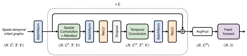
Figure 2: Illustration of the network architecture. The diagram shows the ordering of layers in the STGCN/AAGCN models. The dimensions of the input tensor (including batch), are highlighted underneath those layers that affect them.

3.0.4 Adaptive Graph Convolutional Block.

Adaptive Graph Convolutional Networks (AAGCN) [23] extend STGCN by introducing a learned adaptive graph structure. The adaptive convolution in AAGCN can be expressed as:

$$\textbf{X}_{out}=\sum_{k=1}^{K_{v}}\textbf{W}_{k}\textbf{X}_{in}(\textbf{B}_{k}+\alpha\textbf{C}_{k})$$ (2)

where $\textbf{B}_{k}\in\mathbb{R}^{V\times V}$ represents the global graph learned from data, initialized with the human-body-based adjacency matrix and updated during training without constraints. $\textbf{C}_{k}\in\mathbb{R}^{V\times V}$ is the individual graph adapted to each sample, modulated by a parameterized coefficient $\alpha$ that is unique for each layer. AAGCN incorporates an STC attention module consisting of spatial, temporal, and channel attention mechanisms to enhance its adaptability. Per-sample attention weights are learned to express the importance of joints, time steps, and feature channels, respectively. Each AAGCN block consists of the spatial GCN, including the STC-attention module, followed by a TCN module identical to the STGCN’s.

3.0.5 Network Architecture.

The complete network architecture is shown in Fig. 2. Both the spatial part GCN (including STC for AAGCN), and the TCN are succeeded by a batch normalization (BatchNorm) [11] layer and a rectified linear unit (ReLU) [16] activation layer. To improve training stability and gradient flow, each block includes a residual connection [9]. Additionally, a dropout [24] of 0.5 is added between the GCN and TCN to mitigate overfitting. The network begins with a data BatchNorm layer to normalize the input data. The total number of STGCN or AAGCN blocks is set to 4. The output channel dimensions of these blocks are set at 32, 32, 64, and 64, respectively. Average pooling is applied on the output of the stack of spatio-temporal convolution blocks, which is further entered into a two-layer feedforward network with hidden dimensions 32 and 1, and a ReLU activation in-between.

3.0.6 Training and Implementation.

The training objective is to minimize discrepancy between model predictions and the actual age of the infants. Mean squared error (MSE), $\mathcal{L}=\frac{1}{N}\sum_{i=1}^{N}(\mathrm{a}_{i}-\widehat{\mathrm{a}}_{i})^{2}$, is used as the loss function. Here, $\mathrm{a}_{i}$ represents the actual age of the infant, $\widehat{\mathrm{a}}_{i}$ is the model’s prediction, and $N$ is the number of samples in each batch. The MoMo optimizer [22] with a learning rate of 0.01 was used to minimize the loss function. We employ $k$-fold cross validation with $k=10$ to get a robust assessment of model performance. In each fold, the models are trained for 20 epochs using a batch size of 32, where the best validation checkpoint is stored for each. The models are implemented in the PyTorch Lightning framework [7]. An Nvidia V100 GPU is used for training.

3.0.7 Machine Learning Baseline

As a baseline for our deep learning models, we extend the methodological framework on limb movements established in an earlier study [13], where 20 features based on limb distance, coordination, and global movement quality are constructed for a smaller infant cohort. In addition to linear regression, we apply Random Forest (RF) [2], Gradient Boosting (GB) [8], and eXtreme Gradient Boosting (XGB) [4] predictors. Grid search is implemented for the three latter methods in order to optimize the hyperparameters by minimizing the MSE loss across the cross validation folds over the following grid of values:

• Number of trees/boosting stages: $n\in\{100,300,500,700,900\}$,

• Maximum depth of trees: $d\in\{1,3,5,7,9\}$,

• Learning rate (GB, XGB): $lr\in\{0.1,0.15,0.2,0.25\}$.

The best-performing configurations were identified as RF with $n=300$, $d=7$, GB with $n=300$, $d=1$, $lr=0.2$, and XGB with $n=700$, $d=1$, $lr=0.15$.

4 Results

Table 1: Summary of 10-fold cross validation. The upper part of the table contains regression metrics for the models forming our machine learning baseline, and the lower section shows the performance of the proposed spatio-temporal deep learning models.

Model	RMSE (days)	MAE (days)	MAPE (%)	R2
LR	19.50 $\pm$ 2.49	14.94 $\pm$ 1.61	20.20 $\pm$ 5.74	0.03 $\pm$ 0.23
RF	18.86 $\pm$ 3.39	13.98 $\pm$ 2.57	20.05 $\pm$ 7.17	0.10 $\pm$ 0.23
GB	18.12 $\pm$ 3.56	14.07 $\pm$ 2.85	19.50 $\pm$ 7.36	0.15 $\pm$ 0.26
XGB	18.02 $\pm$ 3.73	14.30 $\pm$ 2.57	19.52 $\pm$ 6.83	0.16 $\pm$ 0.27
STGCN physical	16.76 $\pm$ 2.77	12.12 $\pm$ 1.88	18.30 $\pm$ 5.73	0.28 $\pm$ 0.20
STGCN xy	17.57 $\pm$ 2.70	12.64 $\pm$ 2.74	19.18 $\pm$ 5.62	0.21 $\pm$ 0.18
STGCN	16.63 $\pm$ 2.77	12.34 $\pm$ 2.68	18.30 $\pm$ 5.76	0.29 $\pm$ 0.18
AAGCN	16.30 $\pm$ 2.60	11.61 $\pm$ 2.05	17.42 $\pm$ 5.09	0.32 $\pm$ 0.13

The results of the 10-fold cross-validation are shown in Table 1. We report the average validation RMSE, MAE, MAPE, and R² regression metrics across the folds, along with their standard deviations. The results indicate that the ensemble-based methods outperform the linear model in all metrics, with XGB being the best. The ensemble models also demonstrate a higher variance across folds compared to LR, suggesting a more sensitive response to specific folds.

STGCN physical is trained on infant graphs including only physical connectivity of joints in the body, whereas the rest of the deep learning models are trained also with our proposed connections between limbs illustrated as orange dotted lines in Fig. 1 (b). The additional connections prove favorable for learning developmental age as STGCN performs better than the physical variation across the board. STGCN xy represents a case where the model is trained only on $(x,y)$-components of joint positions. The base STGCN model trained on 3D graphs have 5.7% lower RMSE than the same model trained on 2D data. AAGCN with the completely learned infant graph achieves the best scores with 2.0% lower RMSE than STGCN and 10.6% lower RMSE than XGB.

If we restrict model predictions to infants 10 to 20 weeks, a common age range for GMA studies, regression errors are clearly improved. AAGCN is still the best with RMSE = 11.12 ± 2.92 days. Overall, the prediction of age through the full cohort is challenged most notably by the youngest infants, who are known to express developmentally and qualitatively different selection of spontaneous movement patterns as compared to the typical GMA’s ‘fidgety age’ around three months of age [5].

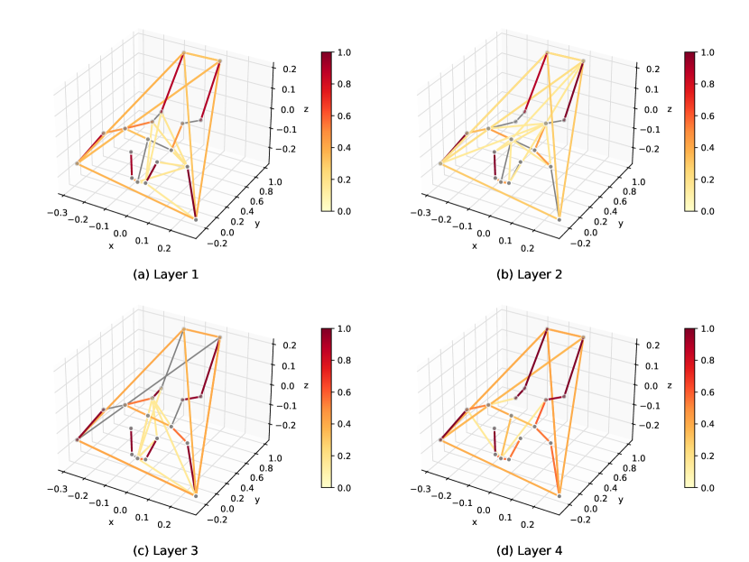
Figure 3: The $|\mathcal{E}|$ strongest connections in the individual adjacency matrix of each layer of the AAGCN model for one input sample. Values are normalized to the range 0 to 1.

The learned graphs in each layer of the AAGCN model as it is adapted to an individual infant is shown in Fig. 3. The subject shown here is a normally developing infant, corrected postnatal age 135 days, that the model predicts as 144 days. Model inference takes 71 ± 12 ms on a CPU. Several new connections are formed in the skeletal graph changing the overall topology significantly. The strongest connections remain as edges from the original input graph, complemented by weak connections between joints further apart in the body. We can see that each layer in the model learn to focus on different body parts. Both the first and second layer emphasize on the lower legs and arms (2nd layer much more on the right arm) for the age assessment. The 3rd and 4th layers put more relative weight on the upper legs that the first two layers. All layers retain most of the bidirectional edges between hands and feet in the top $|\mathcal{E}|$ connections, showing that the coordinated movement of these joints is useful. Most focus overall is put on lower limb movement for determining the age here.

5 Conclusion

In this study, we introduced a data-driven approach utilizing pose-estimated infant recordings to predict age, highlighting the potential advantages of graph neural networks and the efficacy of three-dimensional poses for infant developmental screenings. We show that data-driven methods can extract the relevant features and outperforms machine learning based on limb movement parameters. Expanding the 3D screenings of infant general movements to an even greater scale would be immensely useful for future endeavours as deep learning is known to benefit from more data to enhance performance.

References

- [1] Adde, L., Helbostad, J.L., Jensenius, A.R., Taraldsen, G., Støen, R.: Using computer-based video analysis in the study of fidgety movements. Early Human Development 85(9), 541–547 (2009)
- [2] Breiman, L.: Random forests. Machine Learning 45, 5–32 (2001)
- [3] Chambers, C., Seethapathi, N., Saluja, R., Loeb, H., Pierce, S.R., Bogen, D.K., Prosser, L., Johnson, M.J., Kording, K.P.: Computer vision to automatically assess infant neuromotor risk. IEEE Transactions on Neural Systems and Rehabilitation Engineering 28(11), 2431–2442 (2020)
- [4] Chen, T., Guestrin, C.: XGBoost: A scalable tree boosting system. In: Proceedings of the 22nd ACM SIGKDD International Conference on Knowledge Discovery and Data Mining. pp. 785–794 (2016)
- [5] Einspieler, C., Prechtl, H.F.: Prechtl’s assessment of general movements: a diagnostic tool for the functional assessment of the young nervous system. Mental Retardation and Developmental Disabilities Research Reviews 11(1), 61–67 (2005)
- [6] Einspieler, C., Prechtl, H.F., Ferrari, F., Cioni, G., Bos, A.F.: The qualitative assessment of general movements in preterm, term and young infants—review of the methodology. Early Human Development 50(1), 47–60 (1997)
- [7] Falcon, W., The PyTorch Lightning Team: PyTorch Lightning (1.8.3). https://github.com/Lightning-AI/lightning (2019)
- [8] Friedman, J.H.: Greedy function approximation: A gradient boosting machine. Annals of Statistics pp. 1189–1232 (2001)
- [9] He, K., Zhang, X., Ren, S., Sun, J.: Deep residual learning for image recognition. In: Proceedings of the IEEE Conference on Computer Vision and Pattern Recognition. pp. 770–778 (2016)
- [10] Herskind, A., Greisen, G., Nielsen, J.B.: Early identification and intervention in cerebral palsy. Developmental Medicine & Child Neurology 57(1), 29–36 (2015)
- [11] Ioffe, S., Szegedy, C.: Batch normalization: Accelerating deep network training by reducing internal covariate shift. In: International Conference on Machine Learning. pp. 448–456 (2015)
- [12] Luo, T., Xiao, J., Zhang, C., Chen, S., Tian, Y., Yu, G., Dang, K., Ding, X.: Weakly supervised online action detection for infant general movements. In: International Conference on Medical Image Computing and Computer-Assisted Intervention. pp. 721–731 (2022)
- [13] Marchi, V., Belmonti, V., Cecchi, F., Coluccini, M., Ghirri, P., Grassi, A., Sabatini, A., Guzzetta, A.: Movement analysis in early infancy: Towards a motion biomarker of age. Early Human Development 142, 104942 (2020)
- [14] Marchi, V., Hakala, A., Knight, A., D’Acunto, F., Scattoni, M.L., Guzzetta, A., Vanhatalo, S.: Automated pose estimation captures key aspects of general movements at eight to 17 weeks from conventional videos. Acta Paediatrica 108(10), 1817–1824 (2019)
- [15] McCay, K.D., Ho, E.S., Shum, H.P., Fehringer, G., Marcroft, C., Embleton, N.D.: Abnormal infant movements classification with deep learning on pose-based features. IEEE Access 8, 51582–51592 (2020)
- [16] Nair, V., Hinton, G.E.: Rectified linear units improve restricted boltzmann machines. In: Proceedings of the 27th International Conference on Machine Learning. pp. 807–814 (2010)
- [17] Nguyen-Thai, B., Le, V., Morgan, C., Badawi, N., Tran, T., Venkatesh, S.: A spatio-temporal attention-based model for infant movement assessment from videos. IEEE Journal of Biomedical and Health Informatics 25(10), 3911–3920 (2021)
- [18] Novak, I., Morgan, C., Adde, L., Blackman, J., Boyd, R.N., Brunstrom-Hernandez, J., Cioni, G., Damiano, D., Darrah, J., Eliasson, A.C., et al.: Early, accurate diagnosis and early intervention in cerebral palsy: advances in diagnosis and treatment. JAMA Pediatrics 171(9), 897–907 (2017)
- [19] Rahmati, H., Aamo, O.M., Stavdahl, Ø., Dragon, R., Adde, L.: Video-based early cerebral palsy prediction using motion segmentation. In: 2014 36th Annual International Conference of the IEEE Engineering in Medicine and Biology Society. pp. 3779–3783 (2014)
- [20] Rosenberg, S.A., Zhang, D., Robinson, C.C.: Prevalence of developmental delays and participation in early intervention services for young children. Pediatrics 121(6), e1503–e1509 (2008)
- [21] Sakkos, D., Mccay, K.D., Marcroft, C., Embleton, N.D., Chattopadhyay, S., Ho, E.S.: Identification of abnormal movements in infants: A deep neural network for body part-based prediction of cerebral palsy. IEEE Access 9, 94281–94292 (2021)
- [22] Schaipp, F., Ohana, R., Eickenberg, M., Defazio, A., Gower, R.M.: MoMo: Momentum models for adaptive learning rates. arXiv preprint arXiv:2305.07583 (2023)
- [23] Shi, L., Zhang, Y., Cheng, J., Lu, H.: Skeleton-based action recognition with multi-stream adaptive graph convolutional networks. IEEE Transactions on Image Processing 29, 9532–9545 (2020)
- [24] Srivastava, N., Hinton, G., Krizhevsky, A., Sutskever, I., Salakhutdinov, R.: Dropout: a simple way to prevent neural networks from overfitting. The Journal of Machine Learning Research 15(1), 1929–1958 (2014)
- [25] Stahl, A., Schellewald, C., Stavdahl, Ø., Aamo, O.M., Adde, L., Kirkerod, H.: An optical flow-based method to predict infantile cerebral palsy. IEEE Transactions on Neural Systems and Rehabilitation Engineering 20(4), 605–614 (2012)
- [26] Stevenson, N.J., Oberdorfer, L., Tataranno, M.L., Breakspear, M., Colditz, P.B., de Vries, L.S., Benders, M.J., Klebermass-Schrehof, K., Vanhatalo, S., Roberts, J.A.: Automated cot-side tracking of functional brain age in preterm infants. Annals of Clinical and Translational Neurology 7(6), 891–902 (2020)
- [27] Støen, R., Songstad, N.T., Silberg, I.E., Fjørtoft, T., Jensenius, A.R., Adde, L.: Computer-based video analysis identifies infants with absence of fidgety movements. Pediatric Research 82(4), 665–670 (2017)
- [28] Yan, S., Xiong, Y., Lin, D.: Spatial temporal graph convolutional networks for skeleton-based action recognition. In: Proceedings of the AAAI Conference on Artificial Intelligence. vol. 32 (2018)