Recent advances in chiral EFT based nuclear forces and their applications

Abstract

During the past two decades, chiral effective field theory has evolved into a powerful tool to derive nuclear forces from first principles. Nearly all two-nucleon interactions have been worked out up to sixth order of chiral perturbation theory, while, with few exceptions, three-nucleon forces, which play a subtle, but crucial role in microscopic nuclear structure calculations, have been derived up to fifth order. We review the current status of these forces as well as their applications in nuclear many-body systems. While the ab initio description of light nuclei is generally very successful, we point out and analyze problems encountered with medium-mass nuclei. We also survey the construction of equations of state for symmetric nuclear matter and neutron-rich matter based on chiral forces. A focal point is the symmetry energy and its impact on neutron skins and systems of astrophysical relevance. The physics of neutron-rich systems, from nuclei to compact stars, is essentially determined by the density dependence of the symmetry energy. We review the status of predictions in comparison with latest empirical constraints, with particular attention to those extracted from parity-violating electron scattering.

In loving memory of Ruprecht Machleidt.
His legacy, both human and scientific, will last for decades to come.

1   Introduction

Table 1.1: Abbreviations and acronyms used in this article.

Abbreviation/Acronym	Explanation
ADC(n)	Algebraic diagrammatic construction up to order $n$
AFDMC	Auxiliary-field diffusion Monte Carlo (simulations)
AV18	Argonne $v_{18}$ 2NF [1]
BHF	Brueckner Hartree-Fock (approach)
CC	Coupled cluster (method)
ChPT	Chiral perturbation theory
CMS	Center-of-mass system
CREX	Calcium radius experiment
dof	degrees of freedom
EFT	Effective field theory
EoS	Equation of state
FHNC	Fermi hypernetted chain (method)
FRIB	Facility for Rare Isotope Beams
GFMC	Green’s function Monte Carlo (method)
HF	Hartree-Fock (approximation)
HH	Hyperspherical harmonics (method)
HI	Heavy ion
IANM	Isospin-asymmetric nuclear matter
IM-SRG	In-medium similarity renormalization group (method)
$\Lambda_{b}$	Breakdown scale
LEC	Low-energy constant
LENPIC	Low Energy Nuclear Physics International Collaboration
LO	Leading order
LS	Lippmann-Schwinger
MBPT	Many-body perturbation theory
NCCI	No-core configuration interaction (method)
NCSM	No-core shell model
NLO	Next-to-leading order
NM	Neutron matter
$NN$	Nucleon-nucleon
NNLO, N2LO, N2LO	Next-to-next-to-leading order
N3LO, …	Next-to-next-to-next-to-leading order, …
PREX	Lead (Pb) radius experiment
QCD	Quantum chromodynamics
QMC	Quantum Monte Carlo (methods)
RG	Renormalization group (method)
RMF	Relativistic mean field (approach)
SCGF	Self-consistent Green’s functions (theory)
SNM	Symmetric nuclear matter
SPP	Single-particle potential
SRG	Similarity renormalization group (method)
$T_{\rm lab}$	Laboratory energy
TM	Tucson-Melbourne 3NF [2, 3]
UV14	Urbana $v_{14}$ 2NF [4]
UV	Urbana V 3NF [5]
UIX	Urbana IX 3NF [6]
VMC	Variational Monte Carlo (method)
1PE	One-pion exchange
2PE	Two-pion exchange
3PE	Three-pion exchange
2NF	Two-nucleon force
3NF	Three-nucleon force
4NF	Four-nucleon force

The theory of nuclear forces has a long history. The first serious attempt towards a theory was launched in 1935, when the Japanese physicist Yukawa [7] suggested that nucleons would exchange quanta between each other to create the force. Yukawa constructed his theory in analogy to the theory of the electromagnetic interaction where the exchange of a (massless) photon is the cause of the force. However, in the case of the nuclear force, Yukawa assumed that the mass of the “force-makers” was between the masses of the electron and the proton (which is why these particles were eventually named “mesons”). The mass of the mesons limits the effect of the force to a finite range, since the uncertainty principal allows massive virtual particles to travel only a finite distance. The meson predicted by Yukawa was finally found in 1947 in cosmic ray and in 1948 in the laboratory and called the pion. Yukawa was awarded the Nobel Prize in 1949. In the 1950’s and 60’s more mesons were found in accelerator experiments and the meson theory of nuclear forces was extended to include many mesons. These models became known as one-boson-exchange models, which is a reference to the fact that the different mesons are exchanged singly in this model. The one-boson-exchange model is very successful in explaining essentially all properties of the nucleon-nucleon interaction at low energies [8, 9, 10, 11, 12]. In the 1970’s and 80’s, meson models were developed that went beyond the simple single-particle exchange mechanism. These models included, in particular, the explicit exchange of two pions with all its complications. Well-known representatives of the latter kind are the Paris [13] and the Bonn potentials [14].

Since these meson models were quantitatively very successful, it appeared that they were the solution of the nuclear force problem. However, with the realization (in the 1970’s) that the fundamental theory of strong interactions is quantum chromodynamics (QCD) and not meson theory, all “meson theories” had to be viewed as models, and the attempts to derive the nuclear force from first principals had to start all over again.

The problem with a derivation of nuclear forces from QCD is two-fold. First, each nucleon consists of three valence quarks, quark-antiquark pairs, and gluons such that the system of two nucleons is a complicated many-body problem. Second, the force between quarks, which is created by the exchange of gluons, has the feature of being very strong at the low energy-scale that is characteristic of nuclear physics. This extraordinary strength makes it difficult to find converging expansions. Therefore, during the first round of new attempts, QCD-inspired quark models became popular. The positive aspect of these models is that they try to explain nucleon structure (made up from three constituent quarks) and nucleon-nucleon interactions (six quarks) on an equal footing. Some of the gross features of the two-nucleon force, like the “hard core” are explained successfully in such models. However, from a critical point of view, it must be noted that these quark-based approaches are yet another set of models and not a theory. Alternatively, one may try to solve the six-quark problem with brute computing power, by putting the six-quark system on a four dimensional lattice of discrete points which represents the three dimensions of space and one dimension of time. This method has become known as lattice QCD and is making progress [15, 16]. However, such calculations are computationally very expensive and cannot be used as a standard nuclear physics tool.

Around 1980/90, a major breakthrough occurred when nobel laureate Steven Weinberg applied the concept of an effective field theory (EFT) to low-energy QCD [17, 18, 19]. He simply wrote down the most general theory that is consistent with all the properties of low-energy QCD, since that would make this theory equivalent to low-energy QCD. A particularly important property is the so-called chiral symmetry, which is spontaneously broken. Massless spin-$\frac{1}{2}$ fermions possess the property of chirality, which means that their spin and momentum are either parallel (“right-handed”) or anti-parallel (“left-handed”) and remain so forever. Since the quarks, which nucleons are made of (“up” and “down” quarks), are almost massless, approximate chiral symmetry is a given. Naively, this symmetry should have the consequence that one finds in nature hadrons of the same mass, but with opposite parities (“parity doublets”). However, this is not the case and such failure is termed a spontaneous breaking of the symmetry. According to a theorem first proven by Goldstone, the spontaneous breaking of a symmetry creates a particle, here, the pion. Thus, the pion becomes the main player in the production of the nuclear force. The interaction of pions with nucleons is weak as compared to the interaction of gluons with quarks. Therefore, pion-nucleon processes can be calculated without problem. Moreover, this effective field theory can be expanded in powers of momentum over “scale,” where scale denotes the “chiral symmetry breaking scale” or “breakdown scale.” This scheme is also known as chiral perturbation theory (ChPT) [20, 21, 22] and allows to calculate the various terms that make up the nuclear potential systematically power by power, or order by order [23]. Another advantage of the chiral EFT approach is its ability to generate not only the force between two nucleons, but also many-nucleon forces, on the same footing [24, 25]. In modern theoretical nuclear physics, the chiral EFT approach has gained great popularity and is applied with outstanding success [26, 27, 28].

The purpose of this article is twofold: first, to review the developments of chiral nuclear interactions up to the highest order reached so far (which is the sixth power) and, second, to discuss applications of these forces in the nuclear many-body problem, with emphasis on medium-mass nuclei and neutron-rich systems.

2   Nuclear forces from chiral EFT: Overview

Given an appropriate energy scale, an EFT consists of all interactions consistent with the symmetries that govern the degrees of freedom relevant at that scale. For the problem under consideration, pertinent degrees of freedom are pions (Goldstone bosons), nucleons, and $\Delta(1232)$ isobars. We start out with just pions and nucleons and will discuss the inclusion of the $\Delta(1232)$ isobar later.

2.1   Chiral effective Lagrangians

Schematically, we can write the effective Lagrangian as

$${\cal L}={\cal L}_{\pi\pi}+{\cal L}_{\pi N}+{\cal L}_{NN}+\,\ldots\,,$$ (2.1)

where ${\cal L}_{\pi\pi}$ deals with the dynamics among pions, ${\cal L}_{\pi N}$ describes the interaction between pions and a nucleon, and ${\cal L}_{NN}$ contains two-nucleon contact interactions which consist of four nucleon-fields (four nucleon legs) and no meson fields. The ellipsis stands for terms that involve two nucleons plus pions and three or more nucleons with or without pions, relevant for nuclear many-body forces. Because pion interactions must vanish at zero momentum transfer and in the limit of $m_{\pi}\rightarrow 0$, namely the chiral limit, the Lagrangian is expanded in powers of derivatives or pion masses:

$${\cal L}_{\pi\pi} = {\cal L}_{\pi\pi}^{(2)}+{\cal L}_{\pi\pi}^{(4)}+\ldots\,,$$ (2.2)

$${\cal L}_{\pi N} = {\cal L}_{\pi N}^{(1)}+{\cal L}_{\pi N}^{(2)}+{\cal L}_{\pi N}^{(3)}+{\cal L}_{\pi N}^{(4)}+\ldots,$$ (2.3)

$${\cal L}_{NN} = {\cal L}^{(0)}_{NN}+{\cal L}^{(2)}_{NN}+{\cal L}^{(4)}_{NN}+\ldots\,,$$ (2.4)

where the superscript refers to the number of derivatives or pion mass insertions (chiral dimension) and the ellipsis stands for terms of higher dimensions. We use the heavy-baryon formulation of the Lagrangians, originally proposed by Jenkins and Manohar [29] to study heavy quark systems. The explicit expressions we use can be found in Refs. [26, 30].

2.2   Chiral perturbation theory and power counting

From these Lagrangians, an infinite number of Feynman diagrams can be generated, which seems to make the theory unmanageable. The way out of this dilemma is to design a scheme that makes it possible to organize the diagrams according to their importance. Chiral perturbation theory (ChPT) provides such scheme.

Nuclear potentials are defined by the irreducible types of these graphs. By definition, an irreducible graph is a diagram that cannot be separated into two by cutting only nucleon lines. These graphs are then analyzed in terms of powers of $Q$ with $Q=p/\Lambda_{b}$, where $p$ is generic for a momentum (nucleon three-momentum or pion four-momentum) or a pion mass and $\Lambda_{b}\sim m_{\rho}\sim$ 0.7 GeV is the breakdown scale [31]. Determining the power $\nu$ has become know as power counting.

Following the Feynman rules of covariant perturbation theory, a nucleon propagator is $p^{-1}$, a pion propagator $p^{-2}$, each derivative in any interaction is $p$, and each four-momentum integration $p^{4}$. This is also known as naive dimensional analysis or Weinberg counting.

Since we use the heavy-baryon formalism, we encounter terms which include factors of $p/M_{N}$, where $M_{N}$ denotes the nucleon mass. We count the order of such terms by the rule $p/M_{N}\sim(p/\Lambda_{b})^{2}$, for reasons explained in Refs. [19, 23, 32].

Applying some topological identities, one obtains for the power of a connected irreducible diagram involving $A$ nucleons [26, 18],

$$\nu=-2+2A-2C+2L+\sum_{i}\Delta_{i}\,,$$ (2.5)

with the ‘index of the interaction’ defined by

$$\Delta_{i}\equiv d_{i}+\frac{n_{i}}{2}-2\,.$$ (2.6)

In the above equations: $C$ represents the number of individually connected parts of the diagram while $L$ is the number of loops; moreover, for each vertex $i$, $d_{i}$ indicates how many derivatives or pion masses are present and $n_{i}$ is the number of nucleon fields. The summation extends over all vertices present in that particular diagram. Notice also that chiral symmetry implies $\Delta_{i}\geq 0$. Interactions among pions have at least two derivatives ($d_{i}\geq 2,n_{i}=0$), while interactions between pions and a nucleon have one or more derivatives ($d_{i}\geq 1,n_{i}=2$). Finally, pure contact interactions among nucleons ($n_{i}=4$) have $d_{i}\geq 0$. In this way, a low-momentum expansion based on chiral symmetry can be constructed.

Naturally, the powers must be bounded from below for the expansion to converge. This is in fact the case, with $\nu\geq 0$.

To further illustrate the power formula Eq. (2.5), let us apply it to diagrams shown in Fig. 2.1. From the LO row, we pick the one-pion exchange diagram (second diagram). Each vertex in this disgram is a small dot which consists of one derivative ($d_{i}=1$) and two nucleon legs/fields ($n_{i}=2$); thus, for the small-dot vertices, we have

$$\Delta_{i}=1+\frac{2}{2}-2=0\,.$$ (2.7)

Moreover, $A=2$, $C=1$, and $L=0$, and so Eq. (2.5) results into

$$\nu=-2+2\times 2-2\times 1+2\times 0+\sum_{i}0=0\,,$$ (2.8)

as it should for LO. Moving on to NLO, let us pick one triangular diagram from the second row of Fig. 2.1. All three small-dot vertices in this diagram have $\Delta_{i}=0$. Furthermore, $A=2$, $C=1$, and $L=1$ (one loop). Hence,

$$\nu=-2+2\times 2-2\times 1+2\times 2+\sum_{i}0=2\,,$$ (2.9)

as required for NLO. Alternatively, one can also calculate the power of a diagram ‘from scratch’, i. e., without the help of Eq. (2.5). For the NLO triangular diagram that we just discussed, this goes like this: Each vertex contains one derivative, each meson propagator is (-2), the nucleon propagator is (-1), and the loop integration is 4; thus,

$$\nu=1+1+1-2-2-1+4=2\,,$$ (2.10)

in agreement with what we obtained from Eq. (2.5).

By the way, the power formula Eq. (2.5) also allows to predict the leading orders of connected multi-nucleon forces. Consider a $m$-nucleon irreducibly connected diagram ($m$-nucleon force) in an $A$-nucleon system ($m\leq A$). The number of separately connected pieces is $C=A-m+1$. Inserting this into Eq. (2.5) together with $L=0$ and $\sum_{i}\Delta_{i}=0$ yields $\nu=2m-4$. Thus, two-nucleon forces ($m=2$) appear at $\nu=0$, three-nucleon forces ($m=3$) at $\nu=2$ (but they happen to cancel at that order), and four-nucleon forces at $\nu=4$ (they don’t cancel). More about this in the next sub-section.

For later purposes, we note that for an irreducible $NN$ diagram ($A=2$, $C=1$), the power formula collapses to the very simple expression

$$\nu=2L+\sum_{i}\Delta_{i}\,.$$ (2.11)

To summarize, at each order $\nu$ we only have a well defined, finite number of diagrams, which renders the theory feasible from a practical standpoint. The magnitude of what has been left out at order $\nu$ can be estimated (in a simple way) from $Q^{\nu+1}$ (see Sec. 5, below). The ability to calculate observables (in principle) to any degree of accuracy gives the theory its predictive power.

2.3   The ranking of nuclear forces

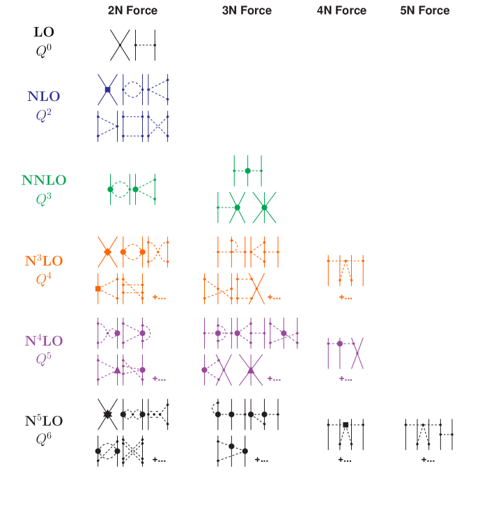
Figure 2.1: Hierarchy of nuclear forces in ChPT. Solid lines represent nucleons and dashed lines pions. Small dots, large solid dots, solid squares, triangles, diamonds, and stars denote vertices of index $\Delta_{i}=\,$ 0, 1, 2, 3, 4, and 6, respectively. Further explanations are given in the text.

Table 2.1: Some basic constants relevant to work reviewed in this article [33]

Quantity		Value
Charged-pion mass $m_{\pi^{\pm}}$		139.5704 MeV
Neutral-pion mass $m_{\pi^{0}}$		134.9768 MeV
Average pion-mass $\bar{m}_{\pi}$		138.0392 MeV
Proton mass $M_{p}$		938.2721 MeV
Neutron mass $M_{n}$		939.5654 MeV
Average nucleon-mass $\bar{M}_{N}$		938.9183 MeV
$\Delta$-isobar mass $M_{\Delta}$		1232 MeV
$\Delta M\equiv M_{\Delta}-\bar{M}_{N}$		293.0817 MeV
Nucleon axial coupling constant $g_{A}$		1.29
$\pi N\Delta$ axial coupling constant $h_{A}$		1.40
Pion-decay constant $f_{\pi}$		92.2 MeV
Conversion constant $\hbar c$		197.32698 MeV fm

As shown in Fig. 2.1, nuclear forces appear in ranked orders in accordance with the power counting scheme.

The lowest power is $\nu=0$, also known as the leading order (LO). At LO we have only two contact contributions with no momentum dependence ($\sim Q^{0}$). They are signified by the four-nucleon-leg diagram with a small-dot vertex shown in the first row of Fig. 2.1. Besides this, we have the static one-pion exchange (1PE), also shown in the first row of Fig. 2.1. Its charge-independent version is given in momentum space by

$$V_{1\pi}({\vec{p}}~{}^{\prime},\vec{p})=-\frac{g_{A}^{2}}{4f_{\pi}^{2}}\>\frac{\vec{\sigma}_{1}\cdot\vec{q}\,\,\vec{\sigma}_{2}\cdot\vec{q}}{q^{2}+m_{\pi}^{2}}\>\bm{\tau}_{1}\cdot\bm{\tau}_{2}\,,$$ (2.12)

where ${\vec{p}}\,^{\prime}$ and $\vec{p}$ denote the final and initial nucleon momenta in the center-of-mass system, respectively. Moreover, $\vec{q}={\vec{p}}\,^{\prime}-\vec{p}\,$ ($q\equiv|\vec{q}|$) is the momentum transfer, and $\vec{\sigma}_{1,2}$ and $\bm{\tau}_{1,2}$ are the spin and isospin operators of nucleon 1 and 2, respectively. Parameters $g_{A}$, $f_{\pi}$, and $m_{\pi}$ denote the axial-vector coupling constant, pion-decay constant, and the pion mass, respectively; see Table 2.1 for their values.

Fourier transform yields the corresponding position-space version of 1PE:

$$\widetilde{V}_{1\pi}(\vec{r})=\frac{g_{A}^{2}\,m_{\pi}^{2}}{48\pi f_{\pi}^{2}}\;\frac{e^{-x}}{r}\left[\vec{\sigma}_{1}\cdot\vec{\sigma}_{2}+\left(1+\frac{3}{x}+\frac{3}{x^{2}}\right)\,S_{12}(\hat{r})\right]\bm{\tau}_{1}\cdot\bm{\tau}_{2}\,$$ (2.13)

with $\vec{r}$ the relative distance between the two nucleons and $x=m_{\pi}\,r$ ($r\equiv|\vec{r}|$).
Moreover,

$$S_{12}(\hat{r})=3\vec{\sigma}_{1}\cdot\hat{r}\,\,\>\vec{\sigma}_{2}\cdot\hat{r}-\vec{\sigma}_{1}\cdot\vec{\sigma}_{2}$$ (2.14)

denotes the standard position-space spin-tensor operator with $\hat{r}=\vec{r}/r$. In Eq. (2.13), a $\delta$-function term has been omitted, since it can be absorbed into the LO contact terms.

In spite of its simplicity, this rough description contains some of the main attributes of the $NN$ force. Through the 1PE it generates the tensor component of the force known to be crucial for the two-nucleon bound state (deuteron). It also predicts correctly $NN$ phase parameters for high partial waves. The two terms which result from a partial-wave expansion of the LO contact terms impact states of zero orbital angular momentum ($S$-waves) and produce attraction at short- and intermediate-range.

Notice that there are no terms with power $\nu=1$, as they would violate parity conservation and time-reversal invariance.

The next order is then $\nu=2$, next-to-leading order, or NLO. The two-pion exchange (2PE) makes its first appearance at this order, and thus it is referred to as the “leading 2PE”. As is well known from decades of nuclear physics, this contribution is essential for a realistic account of the intermediate-range attraction. However, the leading 2PE has insufficient strength, for the following reason: the loops present in the diagrams which involve pions carry the power $\nu=2$ [cf. Eq. (2.11)], and so only $\pi NN$ and $\pi\pi NN$ vertices with $\Delta_{i}=0$ are allowed at this order. These vertices are known to be weak. Moreover, seven new contacts appear at this order which impact $L=0$ and $L=1$ states. (As always, two-nucleon contact terms are indicated by four-nucleon-leg diagrams and a vertex of appropriate shape, in this case a solid square.) At this power, the appropriate operators include central, spin-spin, spin-orbit, and tensor terms, namely all the spin operator structures needed for a realistic description of the two-nucleon force (2NF), although the medium-range attraction still lacks sufficient strength.

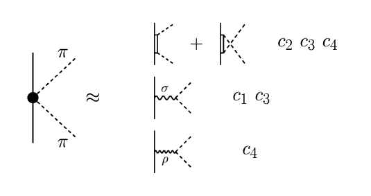
Figure 2.2: Interpretation of the second-order seagull graph (large solid dot) in terms of resonance exchanges. The $c_{i}$ refer to the LECs used in the ${\cal L}_{\pi N}^{(2)}$ Lagrangian.

At the next order, $\nu=3$ or next-to-next-to-leading order (NNLO), the 2PE contains the subleading $\pi\pi NN$ seagull vertices with two derivatives [34]. These vertices, denoted by a large solid dot in Fig. 2.1, simulate correlated 2PE and intermediate $\Delta(1232)$-isobar contributions (cf. Fig. 2.2). Consistent with what the meson theory of the nuclear forces [13, 14] has shown since a long time concerning the importance of these effects, at this order the 2PE finally provides medium-range attraction of realistic strength, bringing the description of the $NN$ force to an almost quantitative level. No new contacts become available at NNLO.

An important advantage of ChPT is that it generates two- and many-nucleon forces on an equal footing. Thus, three-nucleon forces (3NFs) appear for the first time at NLO, but their net contribution vanishes at this order [24]. The first non-zero 3NF contribution is found at NNLO [25, 35]. It is therefore easy to understand why 3NF are very weak as compared to the 2NF which contributes already at $Q^{0}$.

For $\nu=4$, or next-to-next-to-next-to-leading order (N³LO), we display some representative diagrams in Fig. 2.1. There is a large attractive one-loop 2PE contribution (the bubble diagram with two large solid dots), which slightly over-estimates the 2NF attraction at medium range. Two-pion-exchange graphs with two loops are seen at this order, together with three-pion exchange (3PE), which was determined to be very weak at N³LO [36, 37]. The most important feature at this order is the presence of 15 additional contacts $\sim Q^{4}$, signified by the four-nucleon-leg diagram in the figure with the diamond-shaped vertex. These contacts impact states with orbital angular momentum up to $L=2$, and are the reason for the quantitative description of the two-nucleon force (up to approximately 300 MeV in terms of laboratory energy) at this order [26, 38]. More 3NF diagrams show up at N³LO [39, 40], as well as the first contributions to four-nucleon forces (4NF) [41]. We then see that forces involving more and more nucleons appear for the first time at higher and higher orders, which gives theoretical support to the fact that 2NF $\gg$ 3NF $\gg$ 4NF ….

Further 2PE and 3PE occur at N⁴LO (fifth order). The contribution to the 2NF at this order has been first calculated by Entem et al. [42]. It turns out to be moderately repulsive, thus compensating for the attractive surplus generated at N³LO by the bubble diagram with two solid dots. The long- and intermediate-range 3NF contributions at this order have been evaluated [30, 43], but not yet applied in nuclear structure calculations. From the analyses in Refs. [30, 43], one may expect these contributions to be of some importance, as the subleading contributions to the 2P1PE and ring topologies can be understood in terms of $\Delta(1232)$ isobar excitations. Moreover, a new set of 3NF contact terms appears [44] that had a successful application in the context of the so-called ‘$A_{y}$ puzzle’ of nucleon-deuteron scattering [45]. The N⁴LO 4NF has not been derived yet. Because it contains the subleading $\pi\pi NN$ seagull vertex (large solid dot), interpreted in terms of resonance exchanges, see Fig. 2.2, we speculate that this contribution may be non-negligible.

Finally turning to N⁵LO (sixth order): The dominant 2PE and 3PE contributions to the 2NF have been derived by Entem et al. in Ref. [46], which represents the most advanced investigation conducted in chiral EFT for the $NN$ system. The effects are small indicating the desired trend towards convergence of the chiral expansion for the 2NF. Moreover, a new set of 26 $NN$ contact terms $\sim Q^{6}$ occurs that contributes up to $F$-waves (represented by the $NN$ diagram with a star in Fig. 2.1) bringing the total number of $NN$ contacts to 50 [47]. The three-, four-, and five-nucleon forces of this order have not yet been evaluated.

Figure 2.3: Phase-shifts of neutron-proton scattering in $G$ waves at all orders of ChPT from LO to N⁵LO. The filled and open circles represent the results from the Nijmegen multi-energy $np$ phase-shift analysis [48] and the GWU single-energy $np$ analysis SP07 [49], respectively.

To summarize, we show in Fig. 2.3 the contributions to the phase shifts of peripheral $NN$ scattering through all orders from LO to N⁵LO as obtained from a perturbative calculation. Note that the difference between the LO prediction (one-pion-exchange, dotted line) and the data (filled and open circles) is to be provided by two- and three-pion exchanges, i.e. the intermediate-range part of the nuclear force. How well that is accomplished is a crucial test for any theory of nuclear forces. NLO produces only a small contribution, but N²LO creates substantial intermediate-range attraction (most clearly seen in ${}^{1}G_{4}$, ${}^{3}G_{5}$). In fact, N²LO is the largest contribution among all orders. This is due to the one-loop $2\pi$-exchange triangle diagram which involves one $\pi\pi NN$-contact vertex (large solid dot). As discussed, the one-loop $2\pi$-exchange at N²LO is attractive and describes the intermediate-range attraction of the nuclear force about right. At N³LO, more one-loop 2PE is added by the bubble diagram with two large solid dots, a contribution that seemingly is overestimating the attraction. This attractive surplus is then compensated by the prevailingly repulsive two-loop $2\pi$- and $3\pi$-exchanges that occur at N⁴LO and N⁵LO.

In this context, it is worth noting that also in conventional meson theory [14] the one-loop models for the 2PE contribution always show some excess of attraction (cf. Fig. 2 of Ref. [50] and Fig. 10 of Ref. [26]). The same is true for the dispersion theoretic approach pursued by the Paris group (see, e. g., the predictions for ${}^{1}D_{2}$, ${}^{3}D_{2}$, and ${}^{3}D_{3}$ in Fig. 8 of Ref. [51] which are all too attractive). In conventional meson theory, this attraction is reduced by heavy-meson exchanges ($\rho$-, $\omega$-, and $\pi\rho$-exchange) which, however, have no place in chiral effective field theory (as a finite-range contribution). Instead, in the latter approach, two-loop $2\pi$- and $3\pi$-exchanges provide the corrective action.

2.4   Adding the $\Delta$ degree of freedom

Table 2.2: The $\pi N$ LECs as determined in the Roy-Steiner-equation analysis of $\pi N$ scattering conducted in Refs. [52, 53, 54]. The given orders of the chiral expansion refer to the $NN$ system. The $c_{i}$, $\bar{d}_{i}$, and $\bar{e}_{i}$ are the LECs of the second, third, and fourth order $\pi N$ Lagrangian [30], Eq. (2.3), and are in units of GeV^-1, GeV^-2, and GeV^-3, respectively. The uncertainties in the last digits are given in parentheses after the values.

	NNLO		N3LO		N4LO
	$\Delta$-less	$\Delta$-full	$\Delta$-less	$\Delta$-full	$\Delta$-less	$\Delta$-full
$c_{1}$	–0.74(2)	–0.74(2)	–1.07(2)	–1.25(3)	–1.10(3)	–1.11(3)
$c_{2}$	1.81(3)	–0.49(17)	3.20(3)	1.37(16)	3.57(4)	1.52(21)
$c_{3}$	–3.61(5)	–0.65(22)	–5.32(5)	–2.41(23)	–5.54(6)	–1.99(30)
$c_{4}$	2.44(3)	0.96(11)	3.56(3)	1.66(14)	4.17(4)	1.88(19)
$\bar{d}_{1}+\bar{d}_{2}$	—	—	1.04(6)	0.11(11)	6.18(8)	1.75(42)
$\bar{d}_{3}$	—	—	–0.48(2)	–0.81(3)	–8.91(9)	–3.61(48)
$\bar{d}_{5}$	—	—	0.14(5)	0.80(7)	0.86(5)	1.52(7)
$\bar{d}_{14}-\bar{d}_{15}$	—	—	–1.90(6)	–1.04(12)	–12.18(12)	–4.32(79)
$\bar{e}_{14}$	—	—	—	—	1.18(4)	1.67(6)
$\bar{e}_{17}$	—	—	—	—	–0.18(6)	–0.44(6)

The lowest excited state of the nucleon is the $\Delta(1232)$ resonance or isobar (a $\pi$-$N$ $P$-wave resonance with both spin and isospin 3/2) with an excitation energy of $\Delta M=M_{\Delta}-\bar{M}_{N}=293$ MeV. Because of its strong coupling to the $\pi$-$N$ system and low excitation energy, it is an important ingredient for models of pion-nucleon scattering in the $\Delta$-region and pion production from the two-nucleon system at intermediate energies, where the particle production proceeds prevailingly through the formation of $\Delta$ isobars [11]. At low energies, the more sophisticated conventional models for the 2$\pi$-exchange contribution to the $NN$ interaction include the virtual excitation of $\Delta$’s, which in these models accounts for about 50% of the intermediate-range attraction of the nuclear force—as demonstrated by the Bonn potential [14, 55].

Because of its relatively small excitation energy, it is not clear from the outset if, in an EFT, the $\Delta$ should be taken into account explicitly or integrated out as a “heavy” degree of freedom. If it is included, then $\Delta M\sim m_{\pi}$ is considered as another small expansion parameter, besides the pion mass and small external momenta. This scheme has become known as the small scale expansion (SSE) [56]. Note, however, that this extension is of phenomenological character, since $\Delta M$ does not vanish in the chiral limit.

In the chiral EFT discussed so far in this article (also known as the “$\Delta$-less” theory), the effects due to $\Delta$ isobars are taken into account implicitly. Note that the dimension-two $\pi N$ LECs, the $c_{i}$, have unnaturally large values (cf. Table 2.2). The reason for this is that the $\Delta$-isobar (and some meson resonances) contribute considerably to the $c_{i}$—a mechanism that has become known as resonance saturation [57], Fig. 2.2. Therefore, the explicit inclusion of the $\Delta$ (“$\Delta$-full” theory) will take strength out of these LECs and move this strength to a lower order [58, 59, 60, 61]. As a consequence, the convergence of the expansion improves, which is another motivation for introducing explicit $\Delta$-degrees of freedom. We observed that, in the $\Delta$-less theory, the subleading 2PE and 3PE contributions to the 2NF are larger than the leading ones. The promotion of large contributions by one order in the $\Delta$-full theory fixes this problem.

The LECs of the $\pi N$ Lagrangian are usually extracted in the analysis of $\pi$-$N$ scattering data and clearly come out differently in the $\Delta$-full theory as compared to the $\Delta$-less one. While in the $\Delta$-less theory, the magnitude of the LECs $c_{3}$ and $c_{4}$ is about 3-5 GeV^-1 (cf. Table 2.2), they turn out to be around 1 GeV^-1 in the $\Delta$-full theory [54].

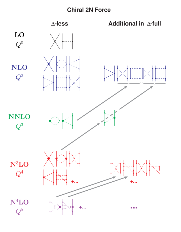
Figure 2.4: Chiral 2NF without and with $\Delta$-isobar degrees of freedom. Arrows indicate the shift of strength when explicit $\Delta$’s are added to the theory. Note that the $\Delta$-full theory consists of the diagrams involving $\Delta$’s plus the $\Delta$-less ones. Double lines represent $\Delta$-isobars; remaining notation as in Fig. 2.1.

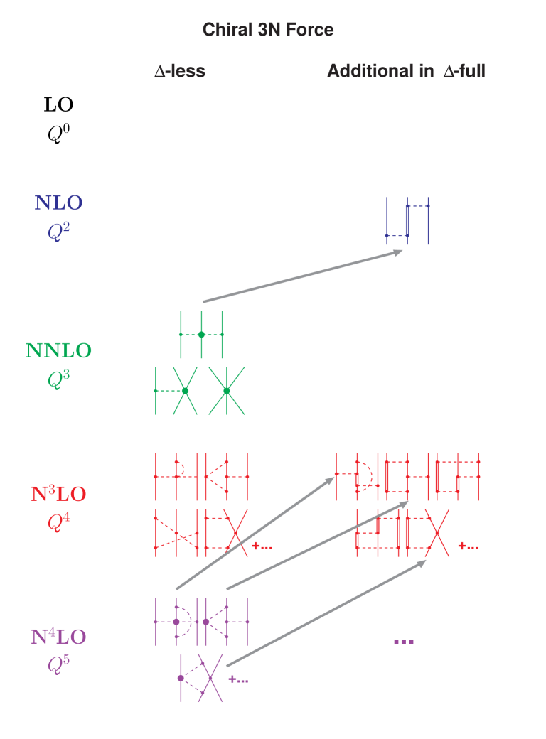
Figure 2.5: The 3NF without and with $\Delta$-isobar degrees of freedom. Arrows indicate the shift of strength when explicit $\Delta$’s are added to the theory. Note that the $\Delta$-full theory consists of the diagrams involving $\Delta$’s plus the $\Delta$-less ones. Double lines represent $\Delta$-isobars; remaining notation as in Fig. 2.1.

In the 2NF, the virtual excitation of $\Delta$-isobars requires at least one loop and, thus, the contribution occurs first at $\nu=2$ (NLO), see Fig. 2.4. The $\Delta$ contributions to the 2PE at NLO were first evaluated in Refs. [23] using time-ordered perturbation theory and later by Kaiser et al. [58] in covariant perturbation theory. The NNLO contributions have been worked out by Krebs et al. [59], who verified the consistency between the $\Delta$-full and $\Delta$-less theories.

The studies of Refs. [58, 59, 62] confirm that a large amount of the intermediate-range attraction of the 2NF is shifted from NNLO to NLO with the explicit introduction of the $\Delta$-isobar. However, it is also found that the NNLO 2PE potential of the $\Delta$-less theory provides a very good approximation to the NNLO potential in the $\Delta$-full theory.

The $\Delta$ isobar also changes the 3NF scenario [60, 61], see Fig. 2.5. The leading 2PE 3NF is promoted to NLO. However, substantial 3NF contributions are expected at N³LO from one-loop diagrams with one, two, or three intermediate $\Delta$-excitations, which correspond to diagrams of order N⁴LO, N⁵LO, and N⁶LO, respectively, in the $\Delta$-less theory. 3NF loop-diagrams with one and two $\Delta$’s are included in the Illinois force [63] in a simplified way.

To summarize, the inclusion of explicit $\Delta$ degrees of freedom does certainly improve the convergence of the chiral expansion by shifting sizable contributions from NNLO to NLO. On the other hand, at NNLO the results for the $\Delta$-full and $\Delta$-less theory are essentially the same. Note that the $\Delta$-full theory consists of the diagrams involving $\Delta$’s plus all diagrams of the $\Delta$-less theory. Thus, the $\Delta$-full theory is much more involved.

The situation could, however, change at N³LO where potentially large contributions enter the picture. It may be more efficient to calculate these terms in the $\Delta$-full theory, because in the $\Delta$-less theory they are spread out over N³LO, N⁴LO and, in part, N⁵LO. These higher order contributions are a crucial test for the convergence of the chiral expansion of nuclear forces and represent a challenging topic for the future. The Bochum group has embarked on such program and has, recently, calculated the 2PE 3NF diagrams involving intermediate $\Delta$-isobar excitations [61].

2.5   The short-range $NN$ force

In previous sections, we mainly discussed the pion-exchange contributions to the $NN$ interaction. They describe the long- and intermediate-range parts of the nuclear force, which are governed by chiral symmetry and rule the peripheral partial waves (cf. Fig. 2.3). However, for a “complete” nuclear force, we have to describe correctly all partial waves, including the lower ones. In fact, in calculations of $NN$ observables at low energies (cross sections, analyzing powers, etc.), the partial waves with $L\leq 2$ are the most important ones, generating the largest contributions. The same is true for microscopic nuclear structure calculations. The lower partial waves are dominated by the dynamics at short distances. Therefore, we need to look now more closely into the short-range part of the $NN$ potential.

In conventional meson theory [11, 14], the short-range nuclear force is described by the exchange of heavy mesons, notably the $\omega(782)$. Qualitatively, the short-distance behavior of the $NN$ potential is obtained by Fourier transform of the propagator of a heavy meson,

$$\int d^{3}q\frac{e^{i{\vec{q}}\cdot{\vec{r}}}}{m^{2}_{\omega}+{\vec{q}}^{2}}\;\sim\;\frac{e^{-m_{\omega}r}}{r}\;.$$ (2.15)

ChPT is an expansion in small momenta $p$, too small to resolve structures like a $\rho(770)$ or $\omega(782)$ meson, because $p\ll\Lambda_{b}\approx m_{\rho,\omega}$. But the latter relation allows us to expand the propagator of a heavy meson into a power series,

$$\frac{1}{m^{2}_{\omega}+p^{2}}\approx\frac{1}{m^{2}_{\omega}}\left(1-\frac{p^{2}}{m^{2}_{\omega}}+\frac{p^{4}}{m^{4}_{\omega}}-+\ldots\right),$$ (2.16)

where the $\omega$ is representative for any heavy meson of interest. The above expansion suggests that it should be possible to describe the short distance part of the nuclear force simply in terms of powers of $p/m_{\omega}$, which fits in well with our over-all power expansion since $p/m_{\omega}\approx p/\Lambda_{b}$. In Fig. 2.1, such terms are denoted by four-nucleon-leg diagrams, like the first diagram in the first and the second row of the figure. Since in these diagrams, the nucleons come infinitely close to each other (no meson-exchanges in-between them that would keep them apart), these diagrams are dubbed contact terms.

Contact terms play an important role in renormalization. Regularization of the loop integrals that occur in multi-pion exchange diagrams typically generates polynomial terms with coefficients that are, in part, infinite or scale dependent (cf. Appendix B of Ref. [26]). Contact terms absorb infinities and remove scale dependences. We also note that contact interactions can be described, qualitatively, using resonance saturation [64].

Due to parity, only even powers of $Q$ are allowed. Thus, the expansion of the contact potential is formally given by

$$V_{\rm ct}=V_{\rm ct}^{(0)}+V_{\rm ct}^{(2)}+V_{\rm ct}^{(4)}+V_{\rm ct}^{(6)}+\ldots\;,$$ (2.17)

where the supersript denotes the power or order. The contact terms of the various orders are given below.

Zeroth order (LO) $NN$ contact potential.

$$V_{\rm ct}^{(0)}(\vec{p^{\prime}},\vec{p})=C_{S}+C_{T}\,\vec{\sigma}_{1}\cdot\vec{\sigma}_{2}$$ (2.18)

and, in terms of partial waves, we have

$$V_{\rm ct}^{(0)}(^{1}S_{0}) = \widetilde{C}_{{}^{1}S_{0}}=4\pi\,(C_{S}-3\,C_{T})\,,$$

$$V_{\rm ct}^{(0)}(^{3}S_{1}) = \widetilde{C}_{{}^{3}S_{1}}=4\pi\,(C_{S}+C_{T})\,.$$ (2.19)

Second order (NLO) $NN$ contact potential.

$$V_{\rm ct}^{(2)}(\vec{p^{\prime}},\vec{p}) = C_{1}\,q^{2}+C_{2}\,k^{2}$$ (2.20)

$$+ \left(C_{3}\,q^{2}+C_{4}\,k^{2}\right)\vec{\sigma}_{1}\cdot\vec{\sigma}_{2}$$

$$+ C_{5}\left(-i\vec{S}\cdot(\vec{q}\times\vec{k})\right)$$

$$+ C_{6}\,(\vec{\sigma}_{1}\cdot\vec{q})\,(\vec{\sigma}_{2}\cdot\vec{q})$$

$$+ C_{7}\,(\vec{\sigma}_{1}\cdot\vec{k})\,(\vec{\sigma}_{2}\cdot\vec{k})$$

with $\vec{k}=(\vec{p^{\prime}}+\vec{p})/2$ and $\vec{S}=(\vec{\sigma}_{1}+\vec{\sigma}_{2})/2$ the total spin.

Partial-wave decomposition yields

$$V_{\rm ct}^{(2)}(^{1}S_{0}) = C_{{}^{1}S_{0}}(p^{2}+{p^{\prime}}^{2})$$

$$V_{\rm ct}^{(2)}(^{3}P_{0}) = C_{{}^{3}P_{0}}\,pp^{\prime}$$

$$V_{\rm ct}^{(2)}(^{1}P_{1}) = C_{{}^{1}P_{1}}\,pp^{\prime}$$

$$V_{\rm ct}^{(2)}(^{3}P_{1}) = C_{{}^{3}P_{1}}\,pp^{\prime}$$

$$V_{\rm ct}^{(2)}(^{3}S_{1}) = C_{{}^{3}S_{1}}(p^{2}+{p^{\prime}}^{2})$$

$$V_{\rm ct}^{(2)}(^{3}S_{1}-^{3}D_{1}) = C_{{}^{3}S_{1}-^{3}D_{1}}p^{2}$$

$$V_{\rm ct}^{(2)}(^{3}D_{1}-^{3}S_{1}) = C_{{}^{3}S_{1}-^{3}D_{1}}{p^{\prime}}^{2}$$

$$V_{\rm ct}^{(2)}(^{3}P_{2}) = C_{{}^{3}P_{2}}\,pp^{\prime}\,,$$ (2.21)

which obviously contributes up to $P$ waves.

Fourth order (N³LO) $NN$ contact potential.

$$V_{\rm ct}^{(4)}(\vec{p^{\prime}},\vec{p}) = D_{1}\,q^{4}+D_{2}\,k^{4}+D_{3}\,q^{2}k^{2}+D_{4}\,(\vec{q}\times\vec{k})^{2}$$ (2.22)

$$+ \left(D_{5}\,q^{4}+D_{6}\,k^{4}+D_{7}\,q^{2}k^{2}+D_{8}\,(\vec{q}\times\vec{k})^{2}\right)\vec{\sigma}_{1}\cdot\vec{\sigma}_{2}$$

$$+ \left(D_{9}\,q^{2}+D_{10}\,k^{2}\right)\left(-i\vec{S}\cdot(\vec{q}\times\vec{k})\right)$$

$$+ \left(D_{11}\,q^{2}+D_{12}\,k^{2}\right)(\vec{\sigma}_{1}\cdot\vec{q})\,(\vec{\sigma}_{2}\cdot\vec{q})$$

$$+ \left(D_{13}\,q^{2}+D_{14}\,k^{2}\right)(\vec{\sigma}_{1}\cdot\vec{k})\,(\vec{\sigma}_{2}\cdot\vec{k})$$

$$+ D_{15}\left(\vec{\sigma}_{1}\cdot(\vec{q}\times\vec{k})\,\,\vec{\sigma}_{2}\cdot(\vec{q}\times\vec{k})\right).$$

The rather lengthy partial-wave expressions at this order are given in Appendix E of Ref. [26]. These contacts affect partial waves up to $D$ waves.

Sixth order (N⁵LO).

At sixth order, 26 new contact terms appear, bringing the total number to 50. These terms as well as their partial-wave decomposition have been worked out in Ref. [47]. They contribute up to $F$-waves. Except for the $F$-wave terms, these contacts have not been used in the construction of $NN$ potentials.

2.6   Regularization and non-perturbative renormalization

Iteration of the potential $\widehat{V}$ in the Lippmann-Schwinger (LS) equation [Eq. (3.4) below] requires cutting $\widehat{V}$ off for high momenta to avoid infinities. This is consistent with the fact that ChPT is a low-momentum expansion which is valid only for momenta $p\ll\Lambda_{b}\approx 0.7$ GeV. Therefore, the potential $\widehat{V}$ is multiplied with a regulator function $f(p^{\prime},p)$,

$${\widehat{V}}(\vec{p}~{}^{\prime},{\vec{p}})\longmapsto{\widehat{V}}(\vec{p}~{}^{\prime},{\vec{p}})\,f(p^{\prime},p)\,.$$ (2.23)

One choice for $f$ is the nonlocal function

$$f(p^{\prime},p)=\exp[-(p^{\prime}/\Lambda)^{2n}-(p/\Lambda)^{2n}]\,,$$ (2.24)

such that

$${\widehat{V}}(\vec{p}~{}^{\prime},{\vec{p}})\,f(p^{\prime},p)\approx{\widehat{V}}(\vec{p}~{}^{\prime},{\vec{p}})\left\{1-\left[\left(\frac{p^{\prime}}{\Lambda}\right)^{2n}+\left(\frac{p}{\Lambda}\right)^{2n}\right]+\ldots\right\}\,,$$ (2.25)

with a cutoff parameter $\Lambda<\Lambda_{b}$.

Equation (2.25) provides an indication of the fact that the exponential cutoff does not necessarily affect the given order at which the calculation is conducted. For sufficiently large $n$, the regulator introduces contributions that are beyond the given order. Assuming a good rate of convergence of the chiral expansion, such orders are small as compared to the given order and, thus, do not affect the accuracy at the given order. (In actual calculations, one uses, of course, the exponential form, Eq. (2.24), and not the expansion Eq. (2.25).)

It is pretty obvious that results for the $T$-matrix may depend sensitively on the regulator and its cutoff parameter. This is acceptable if one wishes to build models. For example, the meson models of the past [11, 14] always depended sensitively on the choices for the cutoff parameters, and they were welcome as additional fit parameters to further improve the reproduction of the $NN$ data. However, the EFT approach wishes to be more fundamental in nature and not just another model.

In field theories, divergent integrals are not uncommon and methods have been devised for how to deal with them. One regulates the integrals and then removes the dependence on the regularization parameters (scales, cutoffs) by renormalization. In the end, the theory and its predictions do not depend on cutoffs or renormalization scales.

Renormalizable quantum field theories, like QED, have essentially one set of prescriptions that takes care of renormalization through all orders. In contrast, EFTs are renormalized order by order, i. e., each order comes with the contact terms needed to renormalize that order. Note that this applies only to perturbative calculations. The $NN$ potential is calculated perturbatively and hence properly renormalized.

However, the story is different for the $NN$ amplitude ($T$-matrix) that results from a solution of the LS equation [Eq. (3.4), below], which is a nonperturbative resummation of the potential. This resummation is necessary in nuclear EFT because nuclear physics is characterized by bound states which are nonperturbative in nature. EFT power counting may be different for nonperturbative processes as compared to perturbative ones. Such difference may be caused by the infrared enhancement of the reducible diagrams generated in the LS equation.

Weinberg’s discussion in Refs. [18, 19] may suggest that the contact terms introduced to renormalize the perturbatively calculated potential, based upon naive dimensional analysis (“Weinberg counting”), may also be sufficient to renormalize the nonperturbative resummation of the potential in the LS equation.

Weinberg’s alleged assumption may not be correct as first pointed out by Kaplan, Savage, and Wise (KSW) [65] who, therefore, suggested to treat 1PE perturbatively—a prescrition which, however, has convergence problems [66]. The KSW critique resulted in a flurry of publications on the renormalization of the $NN$ amplitude, and we refer the interested reader to section 4.5 of Ref. [26] for an account of the first phase of discussion. However, even today, no generally accepted solution to this problem has emerged and some more recent proposals can be found in Refs. [28, 67, 68, 69, 70, 71, 72, 73, 74, 75, 76, 77, 78, 79, 80].

Concerning the construction of quantitative $NN$ potential (by which we mean $NN$ potentials suitable for use in contemporary many-body nuclear methods), only Weinberg counting has been used with success during the past 25 years [23, 38, 81, 82, 83, 84, 85, 86, 87, 88, 89, 90, 91, 92, 93, 94].

In spite of the criticism, Weinberg counting may be perceived as not unreasonable by the following argument. For a successful EFT (in its domain of validity), one must be able to claim independence of the predictions on the regulator within the theoretical error. Also, truncation errors must decrease as we go to higher and higher orders. These are precisely the goals of renormalization.

Lepage [95] has stressed that the cutoff independence should be examined for cutoffs below the hard scale and not beyond. Ranges of cutoff independence within the theoretical error are to be identified using Lepage plots [95].

In Ref. [96], the error of the predictions was quantified by calculating the $\chi^{2}$/datum for the reproduction of the $np$ elastic scattering data as a function of the cutoff parameter $\Lambda$ of the regulator function Eq. (2.24). Predictions by chiral $np$ potentials at order NLO and NNLO were investigated applying Weinberg counting for the $NN$ contact terms. It is found that the reproduction of the $np$ data at lab. energies below 200 MeV is generally poor at NLO, while at NNLO the $\chi^{2}$/datum assumes acceptable values (a clear demonstration of order-by-order improvement). Furthermore, at NNLO, a “plateau” of constant low $\chi^{2}$ for cutoff parameters ranging from about 450 to 850 MeV can be identified. This may be perceived as cutoff independence (and, thus, successful renormalization) for the relevant range of cutoff parameters.

Alternatively, one may go for a compromise between Weinberg’s prescription of full resummation of the potential and Kaplan, Savage, and Wise’s [65] suggestion of perturbative pions—as discussed in Ref. [78]: 1PE is resummed only in lower partial waves and all corrections are included in distorted-wave perturbation theory. However, since current ab initio calculations are tailored such that they need a potential as input, the question is if there is a way to reconcile those (low-cutoff) potentials with the approch of partially perturbative pions. A first attempt to address this issue has recently been undertaken by Valderrama [79].

3   Quantitative chiral $NN$ potentials

3.1   Various representations of $NN$ potentials

We have now rounded up everything needed for a realistic nuclear force—long, intermediate, and short ranged components—and so we can finally proceed to the lower partial waves. However, here we encounter another problem. The two-nucleon system at low angular momentum, particularly in $S$ waves, is characterized by the presence of a shallow bound state (the deuteron) and large scattering lengths. Thus, perturbation theory does not apply. In contrast to $\pi$-$\pi$ and $\pi$-$N$, the interaction between nucleons is not suppressed in the chiral limit ($Q\rightarrow 0$). Weinberg [19] showed that the strong enhancement of the scattering amplitude arises from purely nucleonic intermediate states (“infrared enhancement”). He therefore suggested to use perturbation theory to calculate the $NN$ potential (i.e., the irreducible graphs) and to apply this potential in a scattering equation to obtain the $NN$ amplitude. Current chiral $NN$ potential constructions follow this prescription.

The potential $V$ as discussed in previous sections is, in principal, an invariant amplitude and, thus, satisfies a relativistic scattering equation, for which one may consider the Blankenbecler-Sugar (BbS) equation [97], which reads explicitly,

$${T}({\vec{p}}~{}^{\prime},{\vec{p}})={V}({\vec{p}}~{}^{\prime},{\vec{p}})+\int d^{3}p^{\prime\prime}\>{V}({\vec{p}}~{}^{\prime},{\vec{p}}~{}^{\prime\prime})\>\frac{M_{N}^{2}}{E_{p^{\prime\prime}}}\>\frac{1}{{p}^{2}-{p^{\prime\prime}}^{2}+i\epsilon}\>{T}({\vec{p}}~{}^{\prime\prime},{\vec{p}})$$ (3.1)

with $E_{p^{\prime\prime}}\equiv\sqrt{M_{N}^{2}+{p^{\prime\prime}}^{2}}$ and $M_{N}$ the nuclear mass. The advantage of using a relativistic scattering equation is that it automatically includes relativistic corrections to all orders. Thus, in the scattering equation, no propagator modifications are necessary when raising the order to which the calculation is conducted.

Defining

$$\widehat{V}({\vec{p}}~{}^{\prime},{\vec{p}})\equiv\sqrt{\frac{M_{N}}{E_{p^{\prime}}}}\>{V}({\vec{p}}~{}^{\prime},{\vec{p}})\>\sqrt{\frac{M_{N}}{E_{p}}}$$ (3.2)

and

$$\widehat{T}({\vec{p}}~{}^{\prime},{\vec{p}})\equiv\sqrt{\frac{M_{N}}{E_{p^{\prime}}}}\>{T}({\vec{p}}~{}^{\prime},{\vec{p}})\>\sqrt{\frac{M_{N}}{E_{p}}}\,,$$ (3.3)

the BbS equation collapses into the usual, nonrelativistic LS equation,

$$\widehat{T}({\vec{p}}~{}^{\prime},{\vec{p}})=\widehat{V}({\vec{p}}~{}^{\prime},{\vec{p}})+\int d^{3}p^{\prime\prime}\>\widehat{V}({\vec{p}}~{}^{\prime},{\vec{p}}~{}^{\prime\prime})\>\frac{M_{N}}{{p}^{2}-{p^{\prime\prime}}^{2}+i\epsilon}\>\widehat{T}({\vec{p}}~{}^{\prime\prime},{\vec{p}})\,.$$ (3.4)

Since $\widehat{V}$ satisfies Eq. (3.4), it can be used like a nonrelativistic potential, and $\widehat{T}$ may be perceived as the conventional nonrelativistic $T$-matrix. The above momentum-space equation is equivalent to the nonrelativistic Schrödinger equation, which one would apply for the configuration-space versions of the chiral potentials. Since, for reasons explained in Sec. 3.1.2, below, most practitioners perceive it as desirable to keep configuration-space potentials local, in all chiral $r$-space potentials the approximation is applied:

$$\widehat{V}({\vec{p}}~{}^{\prime},{\vec{p}}) \approx {V}({\vec{p}}~{}^{\prime},{\vec{p}})\,,$$ (3.5)

$$\widehat{T}({\vec{p}}~{}^{\prime},{\vec{p}}) \approx {T}({\vec{p}}~{}^{\prime},{\vec{p}})\,,$$ (3.6)

because the square-root factors in Eqs. (3.2) and (3.3) are nonlocal.

Over the past 20 years, a large number of chiral $NN$ potentials have been constructed and Table 3.1 provides an overview of these activities, which we will discuss now in more detail.

Table 3.1: Chiral $NN$ potentials published during the past 20 years

Year	Authors	Name	Order(s)	$\Delta$’sa	Locality	Cutoff(s)	Max. $T_{lab}$b	$\chi^{2}$/datumc	Ref(s).
Set 1 (Early Birds):
2003	Entem, Machleidt	Idaho	N3LO	No	Nonlocal	500 MeV	300 MeV	1.3	[38]
2005	Epelbaum et al.	Bochum	N3LO	No	Nonlocal	450, 600 MeV	300 MeV	14.5, 2.3	[82]
Set 2 (Göteborg/Oak Ridge):
2013	Ekström et al.	NNLOopt	NNLO	No	Nonlocal	500 MeV	290 MeV	9.5	[85]
2015	Ekström et al.	NNLOsat	NNLO	No	Nonlocal	450 MeV	35 MeV	39.0d, 42.7e	[92]
2018	Ekström et al.	$\Delta$NNLO	NNLO	Yes	Nonlocal	450 MeV	200 MeV	25.1f	[93]
2020	Jiang, Ekström et al.	$\Delta$NNLOGO	NNLO	Yes	Nonlocal	394, 450 MeV	200 MeV	32.6f, 29.6f	[98]
Set 3 (Configuration space):
2014	Gezerlis et al.		LO-NNLO	No	Local	1.0-1.2 fm	250 MeV	12.2g	[86]
2015	Piarulli et al.		NNLO/N3LOh	Yes	Min. nonloc.i	0.8-1.2 fm	300 MeV	1.35(2)	[87]
2016	Piarulli et al.	Norfolk, NV2	LO-N(3)LOh	Yes	Local	0.8-1.2 fm	200 MeV	1.40j	[88]
2023	Saha et al.	Idaho	LO-N3LO	No	Local	1.0-1.2 fm	200 MeV	1.45k	[99]
2023	Somasundaram et al.	LO-N3LOLA	LO-N3LO	No	Max. locall	0.6-0.9 fm	400 MeV		[100]
Set 4 (Latest high accuracy and high precision):
2015	Epelbaum et al.	LENPIC	LO-N4LO	No	Semilocalm	0.8-1.2 fm	300 MeV		[83, 84]
2017	Entem et al.	Idaho	LO-N4LO	No	Nonlocal	450-550 MeV	300 MeV	1.15n	[94]
2018	Reinert et al.	LENPIC	LO-N4LO+	No	Semilocalm	350-550 MeV	300 MeV	1.03p	[91]
2021	Nosyk et al.	Idaho	LO-NNLO	Yes	Nonlocal	394, 450 MeV	200 MeV	3.71q	[62]

^a $\Delta(1232)$-isobar excitations included, yes or no?
^b Maximum lab. energy up to which $NN$ phase shifts or data are fitted.
^c $\chi^{2}$/datum for the reproduction of the $NN$ data up to pion-production threshold—unless noted otherwise.
^d $\chi^{2}$/datum for the $NN$ data up to 100 MeV.
^e $\chi^{2}$/datum for the $NN$ data up to 190 MeV.
^f $\chi^{2}$/datum for the $NN$ data up to 200 MeV.
^g $\chi^{2}$/datum for the $NN$ data up to 190 MeV for the NNLO potential with cutoff 1.0 fm.
^h 2PE at NNLO, contacts at N³LO.
ⁱ Minimally nonlocal.
^j $\chi^{2}$/datum for the $NN$ data up to 200 MeV for the N(3)LO potential with cutoff 0.8 fm.
^k $\chi^{2}$/datum for the $NN$ data up to 190 MeV for the N³LO potential with cutoff 1.0 fm.
^l Maximally local.
^m Pion-exchanges local, contacts nonlocal.
ⁿ For the N⁴LO potential with cutoff 500 MeV.
^p For the N⁴LO⁺ potential with cutoff 450 MeV.
^q $\chi^{2}$/datum for the $NN$ data up to 200 MeV for the $\Delta$NNLO potential with cutoff 450 MeV.

3.1.1   Momentum space potentials

Since ChPT is a low-momentum expansion, the most natural way to construct a chiral $NN$ potential is in momentum space. Therefore, the first quantitative chiral $NN$ potentials—the ($\Delta$-less) N³LO “Early Birds” potentials [38, 82] (cf. Table 3.1)—as well as the latest high accuracy and high precision potentials at N⁴LO [83, 94, 91] are all represented in momentum space. Differences between these potentials have mainly to do with the types of regulators applied. While all Idaho potentials [38, 94] and the older Bochum potentials [82] use the nonlocal regulator function Eq. (2.24) for contacts as well as pion-exchanges, the more recent Bochum potentials [83, 91] apply local procedures to the pion-exchange contributions to reduce the impact of finite-cutoff artifacts.

Also the $\Delta$-full theory has been invoked for the construction of $NN$ potentials. The Göteborg/Oak Ridge group has constructed families of NNLO potentials of this kind [93, 98]. Unfortunately, these $\Delta$-full NNLO potentials by the Göteborg/Oak Ridge group severely lack accuracy as does their $\Delta$-less predecessor [92]—with $\chi^{2}$/datum between 30 and 40, which is unacceptable (cf. the “Set 2” of Table 3.1). Consequently, their predictions for nuclear many-body systems are unreliable and even misleading, as discussed in detail in Ref. [62], see also Sec. 6.1.2, below. It has also been demonstrated that, at least at NNLO, there is no advantage to the $\Delta$-full theory as compared to the $\Delta$-less one [62].

3.1.2   Configuration space potentials

Chiral $NN$ potentials have also been constructed in configuration space (position space, “$r$-space”), see “Set 3” of Table 3.1. The main motivation for their construction is that some ab initio few- and many-body algorithms, particularly, the ones known as quantum Monte Carlo (QMC) methods [101, 102] require local $r$-space potentials as their input. Variational Monte Carlo (VMC) and Green’s Function Monte Carlo (GFMC) techniques provide reliable solutions of the many-body Schrődinger equation for, presently, up to 12 nucleons. Spectra, form factors, transitions, low-energy scattering, and response functions for light nuclei have been successfully calculated using QMC methods [103]. A further extension, the Auxiliary Field Diffusion Monte Carlo (AFDMC) [101, 102], additionally samples the spin-isospin degrees of freedom, thus, making possible the study of neutron matter (NM). In summary, QMC techniques have substantially contributed to the progress in ab initio nuclear structure of the past 20+ years, and will continue to do so. Thus, high-quality nuclear interactions suitable for application by these promising many-body methods are called for.

The first chiral $NN$ potential ever constructed was, in fact, represented in configuration space (a $\Delta$-full NLO potential [23]). About 20 years later, a local $\Delta$-less NNLO was developed [86]. A more accurate one followed soon after that was constructed in the hybrid format, NNLO/N³LO [87, 88], where $\Delta$-full 2PE contributions are included up to NNLO and contact terms up to N³LO. A chiral $r$-space potential up to order N³LO was recently developed. This construction is consistent in the sense that the same power counting scheme and cutoff procedures are applied at all orders. The contacts and ($\Delta$-less) pion-exchanges are all taken into account up to N³LO [99]. A maximally local potential at N3LO in $\Delta$-less chiral EFT is under construction by the Los Alamos theory group [100]. N3LO in delta-less chiral EFT. Our interactions include a total of 21 contact operators at N3LO, out of which four are nonlocal.

The pion-exchange contributions up to N³LO are all local from the outset [99]. To preserve the local character, the pion-exchanges are multiplied with local regulator functions, which suppress the potential at short distances, at which the 2PE expressions diverge up to $\sim 1/r^{7}$. Commonly used local regulators are

$$\widetilde{f}_{1}(r) = 1-\exp\left[-\left(\frac{r}{R_{\pi}}\right)^{2n}\right]\,,$$ (3.7)

$$\widetilde{f}_{2}(r) = \left[1-\exp\left(-\frac{r^{2}}{R_{\pi}^{2}}\right)\right]^{n}\,,$$ (3.8)

$$\widetilde{f}_{3}(r) = 1-\frac{1}{\left({r}/{R_{\pi}}\right)^{6}\,\exp\left[{2(r-R_{\pi})}/{R_{\pi}}\right]\,+\,1}\,.$$ (3.9)

Regulator $\widetilde{f}_{1}$ is used in Ref. [86] with $n=2$. Regulator $\widetilde{f}_{2}$ is applied in Refs. [83, 100] with $n=6$. Reference [99] takes a more distinct approach and (using $n=5$) employs $\widetilde{f}_{2}$ to the 2PE contributions, while utilizing $\widetilde{f}_{1}$ for 1PE, to preserve the beneficial nature of the 1PE also in the intermediate range. Finally, $\widetilde{f}_{3}$ is chosen for the potentials by Piarulli et al. [87, 88]. To provide an idea of the differences between the regulators, we show in Fig. 3.1 the shape of the different functions for $R_{\pi}=1.0$ fm and $n=5$. In summary, in all configuration-space potentials, the regularized pion-exchange contributions are strictly local—and there is no problem achieving this.

Figure 3.1: Various regulator functions applied to the pion-exchange contributions of chiral position-space potentials. The solid, dashed, and dotted curves represent the regulators $\widetilde{f}_{1}(r)$, $\widetilde{f}_{2}(r)$, and $\widetilde{f}_{3}(r)$ given in Eqs. (3.7), (3.8), and (3.9), respectively, with $n=5$ and $R_{\pi}=1.0$.

In contrast, the locality of the contact terms is a more involved issue, which we will discuss now. In principle, the most general set of contact terms at each order is provided by all combinations of spin, isospin, and momentum operators that are allowed by the usual symmetries [104] at the given order. Two momenta are available, namely, the final and initial nucleon momenta in the center-of-mass system, ${\vec{p}}\,^{\prime}$ and $\vec{p}$. This can be reformulated in terms of two alternative momenta, viz., the momentum transfer $\vec{q}={\vec{p}}\,^{\prime}-\vec{p}$ and the average momentum $\vec{k}=({\vec{p}}\,^{\prime}+\vec{p})/2$. Functions of $\vec{q}$  lead to local interactions, that is, to functions of the relative distance ${\vec{r}}$ between the two nucleons after Fourier transform. On the other hand, functions of $\vec{k}$ lead to gradient operators ($-i\nabla$) and, thus, nonlocal interactions.

As discussed, chiral potentials are multiplied by a regulator function that suppresses the large momenta (or, equivalently, the short distances). Depending on the type of momenta used, the regulator can be local or nonlocal.

When chiral $NN$ potentials are constructed in momentum-space and regulated by nonlocal cutoff functions, like Eq. (2.24), then it is possible to reduce the number of contact operators (by a factor of two) due to Fierz ambiguity [105], which is a consequence of the fact that nucleons are Fermions and obey the Pauli exclusion principle. The momentum-space contact terms shown in Eqs. (2.18), (2.20), and (2.22) are all Fierz reduced.

However, when a local (regulator) function is applied to the contact terms, then the Fierz rearrangement freedom is violated [105, 99]. For example, consider a contact operator of order zero ($\sim Q^{0}$, LO). After a partial-wave decomposition and when multiplied by either no regulator or a nonlocal regulator, such operator produces no contributions for states with orbital angular momentum $L>0$, i.e., $P$ and higher partial waves. However, this property is violated when the operator is multiplied with a local regulator function [105, 99]. Attempts can be undertaken to partially restore Fierz reordering as tried in Ref. [105] by way of contributions of higher order. Based upon this argument, some local potentials assume Fierz reordering for their contacts [86, 87, 88, 100].

Alternatively, one may argue that it does not make sense to apply a symmetry that is invalid for the problem under consideration, and simply use for the contacts all combinations of spin, isospin, angular momentum, and momentum $\vec{q}$ that are allowed by the usual symmetries—in each of the given orders. This attitude was taken for the local potentials of Ref. [99]. On a historical note, this is also the approach that was used for the very first chiral $NN$ potentials ever constructed [23].

Ignoring Fierz reordering, the LO or zeroth order charge-independent contact terms are given in momentum-space by [99]

$${V}_{\rm ct}^{(0)}(q)\, = \,\left(C_{c}\,+C_{\tau}\,\bm{\tau}_{1}\cdot\bm{\tau}_{2}\,+\,C_{\sigma}\,\vec{\sigma}_{1}\cdot\vec{\sigma}_{2}\,+\,C_{\sigma\tau}\,\vec{\sigma}_{1}\cdot\vec{\sigma}_{2}\;\bm{\tau}_{1}\cdot\bm{\tau}_{2}\right)\,f_{\rm ct}(q)\,,$$ (3.10)

while, with Fierz reordering, only two of these terms are retained, e.g., the ones shown in Eq. (2.18) [86, 87, 88, 100].

To maintain the local nature, the contacts are multiplied with a local regulator function for which, in the case of most configuration-space potentials [87, 88, 99, 100], a local Gaussian is chosen,

$$f_{\rm ct}(q)=e^{-(q/\Lambda)^{2}}\,,$$ (3.11)

simply for practical reasons, because the Fourier transform of a Gaussian is a Gaussian, that is

$$\widetilde{f}_{\rm ct}(r)=\frac{1}{\pi^{3/2}\,R_{\rm ct}^{3}}\,e^{-(r/R_{\rm ct})^{2}}\,.$$ (3.12)

The relationship between momentum-space cutoff $\Lambda$ and position-space cutoff $R_{\rm ct}$ is then

$$R_{\rm ct}=2/\Lambda\,.$$ (3.13)

Note that we use units such that $\hbar=c=1$.

Moving up to subleading orders, additional problems occur because the Fourier transforms of some of the momentum-space contacts at second order, Eq. (2.20), and fourth order, Eq. (2.22), are nonlocal. However, at second order, an alternative set of seven linear independent local operators can be found [86, 87, 88, 105, 99, 100], namely

$${V}_{\rm ct}^{(2)}({\vec{p}}~{}^{\prime},\vec{p})\, = \Big{\{}\left(\widetilde{C}_{1}\,+\widetilde{C}_{2}\,\bm{\tau}_{1}\cdot\bm{\tau}_{2}\,+\,\widetilde{C}_{3}\,\vec{\sigma}_{1}\cdot\vec{\sigma}_{2}\,+\,\widetilde{C}_{4}\,\vec{\sigma}_{1}\cdot\vec{\sigma}_{2}\;\bm{\tau}_{1}\cdot\bm{\tau}_{2}\right)\,q^{2}$$ (3.14)

$$+\left(\widetilde{C}_{5}\,+\widetilde{C}_{6}\,\bm{\tau}_{1}\cdot\bm{\tau}_{2}\,\right)\,\widehat{S}_{12}(\vec{q})\;\;$$

$$+\,\,\,\widetilde{C}_{7}\,\,\left[-i\vec{S}\cdot(\vec{q}\times\vec{k})\,\right]\Big{\}}\,f_{\rm ct}(q)\,,$$

where

$$\widehat{S}_{12}(\vec{q})=3\,\vec{\sigma}_{1}\cdot\vec{q}\,\,\>\vec{\sigma}_{2}\cdot\vec{q}-q^{2}\,\vec{\sigma}_{1}\cdot\vec{\sigma}_{2}$$ (3.15)

is the spin-tensor operator in momentum-space. Note that some models [99] include an eighth term, $\widetilde{C}_{8}\,\bm{\tau}_{1}\cdot\bm{\tau}_{2}\,\left[-i\vec{S}\cdot(\vec{q}\times\vec{k})\,\right]$, for convenience.

Fourier transform of Eq. (3.14) creates the second order local contact contribution in position space

$$\widetilde{V}_{\rm ct}^{(2)}(\vec{r})\, = \,\left(\widetilde{C}_{1}\,+\widetilde{C}_{2}\,\bm{\tau}_{1}\cdot\bm{\tau}_{2}\,+\,\widetilde{C}_{3}\,\vec{\sigma}_{1}\cdot\vec{\sigma}_{2}\,+\,\widetilde{C}_{4}\,\vec{\sigma}_{1}\cdot\vec{\sigma}_{2}\;\bm{\tau}_{1}\cdot\bm{\tau}_{2}\right)\,\,^{\rm ct}\widetilde{V}_{C}^{(2)}(r)$$ (3.16)

$$+\left(\widetilde{C}_{5}\,+\widetilde{C}_{6}\,\bm{\tau}_{1}\cdot\bm{\tau}_{2}\,\right)\,S_{12}(\hat{r})\;\;^{\rm ct}\widetilde{V}_{T}^{(2)}(r)$$

$$+\,\,\,\widetilde{C}_{7}\,\,\,(\vec{L}\cdot\vec{S})\;\;^{\rm ct}\widetilde{V}_{LS}^{(2)}(r)\,,$$

where $\vec{L}$ denotes the operator of total angular momentum. Furthermore,

$${}^{\rm ct}\widetilde{V}_{C}^{(2)}(r) = -\widetilde{f}_{\rm ct}^{(2)}(r)-\frac{2}{r}\,\widetilde{f}_{\rm ct}^{(1)}(r)\,,$$ (3.17)

$${}^{\rm ct}\widetilde{V}_{T}^{(2)}(r) = -\widetilde{f}_{\rm ct}^{(2)}(r)+\frac{1}{r}\,\widetilde{f}_{\rm ct}^{(1)}(r)\,,$$ (3.18)

$${}^{\rm ct}\widetilde{V}_{LS}^{(2)}(r) = -\frac{1}{r}\,\widetilde{f}_{\rm ct}^{(1)}(r)\,,$$ (3.19)

with

$$\widetilde{f}_{\rm ct}^{(n)}(r)=\frac{d^{n}\widetilde{f}_{\rm ct}(r)}{dr^{n}}\,.$$ (3.20)

Turning now to the N³LO or fourth order contact contributions, we have, when Fierz reordering is ignore and only the local momentum $q$ taken into account [99],

$${V}_{\rm ct}^{(4)}({\vec{p}}~{}^{\prime},\vec{p})\, = \Big{\{}\left(\widetilde{D}_{1}\,+\widetilde{D}_{2}\,\bm{\tau}_{1}\cdot\bm{\tau}_{2}\,+\,\widetilde{D}_{3}\,\vec{\sigma}_{1}\cdot\vec{\sigma}_{2}\,+\,\widetilde{D}_{4}\,\vec{\sigma}_{1}\cdot\vec{\sigma}_{2}\;\bm{\tau}_{1}\cdot\bm{\tau}_{2}\right)\,q^{4}$$ (3.22)

$$+\left(\widetilde{D}_{5}\,+\widetilde{D}_{6}\,\bm{\tau}_{1}\cdot\bm{\tau}_{2}\,\right)\,q^{2}\,\widehat{S}_{12}(\vec{q})\;\;$$

$$+\left(\widetilde{D}_{7}\,+\widetilde{D}_{8}\,\bm{\tau}_{1}\cdot\bm{\tau}_{2}\,\right)\,q^{2}\,\left[-i\vec{S}\cdot(\vec{q}\times\vec{k})\,\right]\;\;$$

$$+\left(\widetilde{D}_{9}\,+\widetilde{D}_{10}\,\bm{\tau}_{1}\cdot\bm{\tau}_{2}\,\right)\,\left[-i\vec{S}\cdot(\vec{q}\times\vec{k})\,\right]^{2}$$

$$+\,\left(\widetilde{D}_{11}\,+\widetilde{D}_{12}\,\bm{\tau}_{1}\cdot\bm{\tau}_{2}\,+\,\widetilde{D}_{13}\,\vec{\sigma}_{1}\cdot\vec{\sigma}_{2}\,+\,\widetilde{D}_{14}\,\vec{\sigma}_{1}\cdot\vec{\sigma}_{2}\;\bm{\tau}_{1}\cdot\bm{\tau}_{2}\right)\,\,\left[-i(\vec{q}\times\vec{k})\,\right]^{2}\Big{\}}f_{\rm ct}(q)\,,$$

which converts to

$$\widetilde{V}_{\rm ct}^{(4)}(\vec{r})\, = \,\left(\widetilde{D}_{1}\,+\widetilde{D}_{2}\,\bm{\tau}_{1}\cdot\bm{\tau}_{2}\,+\,\widetilde{D}_{3}\,\vec{\sigma}_{1}\cdot\vec{\sigma}_{2}\,+\,\widetilde{D}_{4}\,\vec{\sigma}_{1}\cdot\vec{\sigma}_{2}\;\bm{\tau}_{1}\cdot\bm{\tau}_{2}\right)\,\,^{\rm ct}\widetilde{V}_{C}^{(4)}(r)$$ (3.23)

$$+\left(\widetilde{D}_{5}\,+\widetilde{D}_{6}\,\bm{\tau}_{1}\cdot\bm{\tau}_{2}\,\right)\,S_{12}(\hat{r})\;\;^{\rm ct}\widetilde{V}_{T}^{(4)}(r)$$

$$+\left(\widetilde{D}_{7}\,+\widetilde{D}_{8}\,\bm{\tau}_{1}\cdot\bm{\tau}_{2}\,\right)\,(\vec{L}\cdot\vec{S})\;\;^{\rm ct}\widetilde{V}_{LS}^{(4)}(r)$$

$$+\left(\widetilde{D}_{9}\,+\widetilde{D}_{10}\,\bm{\tau}_{1}\cdot\bm{\tau}_{2}\,\right)\,(\vec{L}\cdot\vec{S})^{2}\;\;{}^{\rm ct}\widetilde{V}_{LS2}^{(4)}(r)$$

$$+\,\left(\widetilde{D}_{11}\,+\widetilde{D}_{12}\,\bm{\tau}_{1}\cdot\bm{\tau}_{2}\,+\,\widetilde{D}_{13}\,\vec{\sigma}_{1}\cdot\vec{\sigma}_{2}\,+\,\widetilde{D}_{14}\,\vec{\sigma}_{1}\cdot\vec{\sigma}_{2}\;\bm{\tau}_{1}\cdot\bm{\tau}_{2}\right)\,\,{\vec{L}}^{2}\,{}^{\rm ct}\widetilde{V}_{LL}^{(4)}(r)\,,$$

with

$${}^{\rm ct}\widetilde{V}_{C}^{(4)}(r) = \widetilde{f}_{\rm ct}^{(4)}(r)+\frac{4}{r}\,\widetilde{f}_{\rm ct}^{(3)}(r)\,,$$ (3.24)

$${}^{\rm ct}\widetilde{V}_{T}^{(4)}(r) = \widetilde{f}_{\rm ct}^{(4)}(r)+\frac{1}{r}\,\widetilde{f}_{\rm ct}^{(3)}(r)-\frac{6}{r^{2}}\,\widetilde{f}_{\rm ct}^{(2)}(r)+\frac{6}{r^{3}}\,\widetilde{f}_{\rm ct}^{(1)}(r)\,,$$ (3.25)

$${}^{\rm ct}\widetilde{V}_{LS}^{(4)}(r) = \frac{1}{r}\,\widetilde{f}_{\rm ct}^{(3)}(r)+\frac{2}{r^{2}}\,\widetilde{f}_{\rm ct}^{(2)}(r)-\frac{2}{r^{3}}\,\widetilde{f}_{\rm ct}^{(1)}(r)\,,$$ (3.26)

$${}^{\rm ct}\widetilde{V}_{LS2}^{(4)}(r) = \frac{1}{r^{2}}\,\widetilde{f}_{\rm ct}^{(2)}(r)-\frac{1}{r^{3}}\,\widetilde{f}_{\rm ct}^{(1)}(r)\,,$$ (3.27)

$${}^{\rm ct}\widetilde{V}_{LL}^{(4)}(r) = \frac{1}{r^{2}}\,\widetilde{f}_{\rm ct}^{(2)}(r)-\frac{1}{r^{3}}\,\widetilde{f}_{\rm ct}^{(1)}(r)\,,$$ (3.28)

where, from the Fourier transforms of Eqs. (3.22) and (3.22), only the local terms are retained [87, 99].

However, at fourth order, the full scenario is more complicated than this. With Fierz reordering, there should be 15 linear independent operators, cf. Eq. (2.22). But there exist only 11 linearly independent local ones (in the above, the $\widetilde{D}_{10}$, $\widetilde{D}_{12}$, and $\widetilde{D}_{14}$ terms are redundant for strict Fierz reordering). As a consequence, one finds two different philosophies in local N³LO potential constructs: One is to insist the potential to be strictly local and, thus, use only the 11 local ones [88] (or all of the above 14 ones [99]). In the alternative approach, one insists on using a complete set of 15 operators and, hence, includes four nonlocal ones. Hoping that the nonlocal terms are small, their contributions can be included in perturbation theory, thus, making QMC calculations possible. This attitude is assumed in Refs. [87, 100], which explains the attributes “minimally nonlocal” or “maximally local” used to characterize these potentials.

The operator set used in Eq. (3.23) is the same that the phenomenological Argonne $v_{18}$ potential (AV18) [1] is based upon. Thus, for local chiral potentials applying this set, a detailed comparison with established phenomenology can be made. Such comparison, conducted in Ref. [99], revealed substantial agreement between the AV18 and the chiral N³LO potentials in the intermediate range ruled by chiral symmetry, hence, providing a chiral underpinning for the phenomenological AV18 potential.

3.2   $NN$ potentials order by order

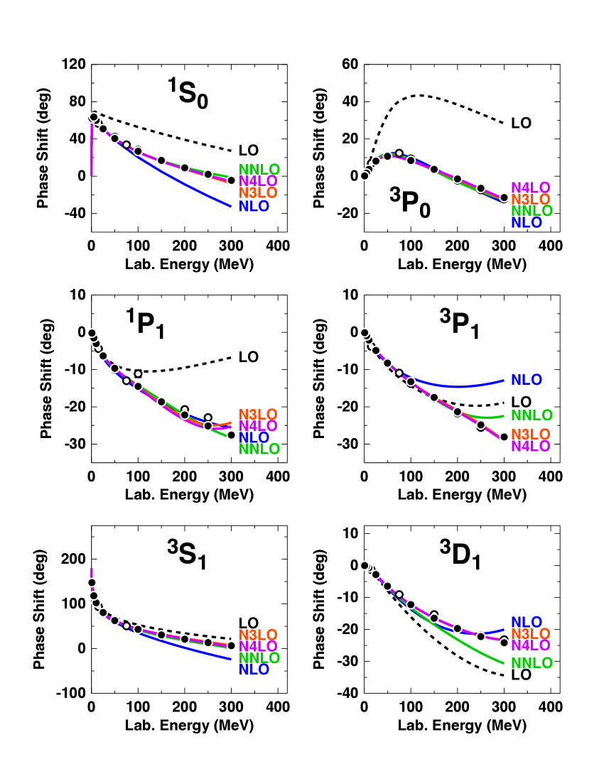
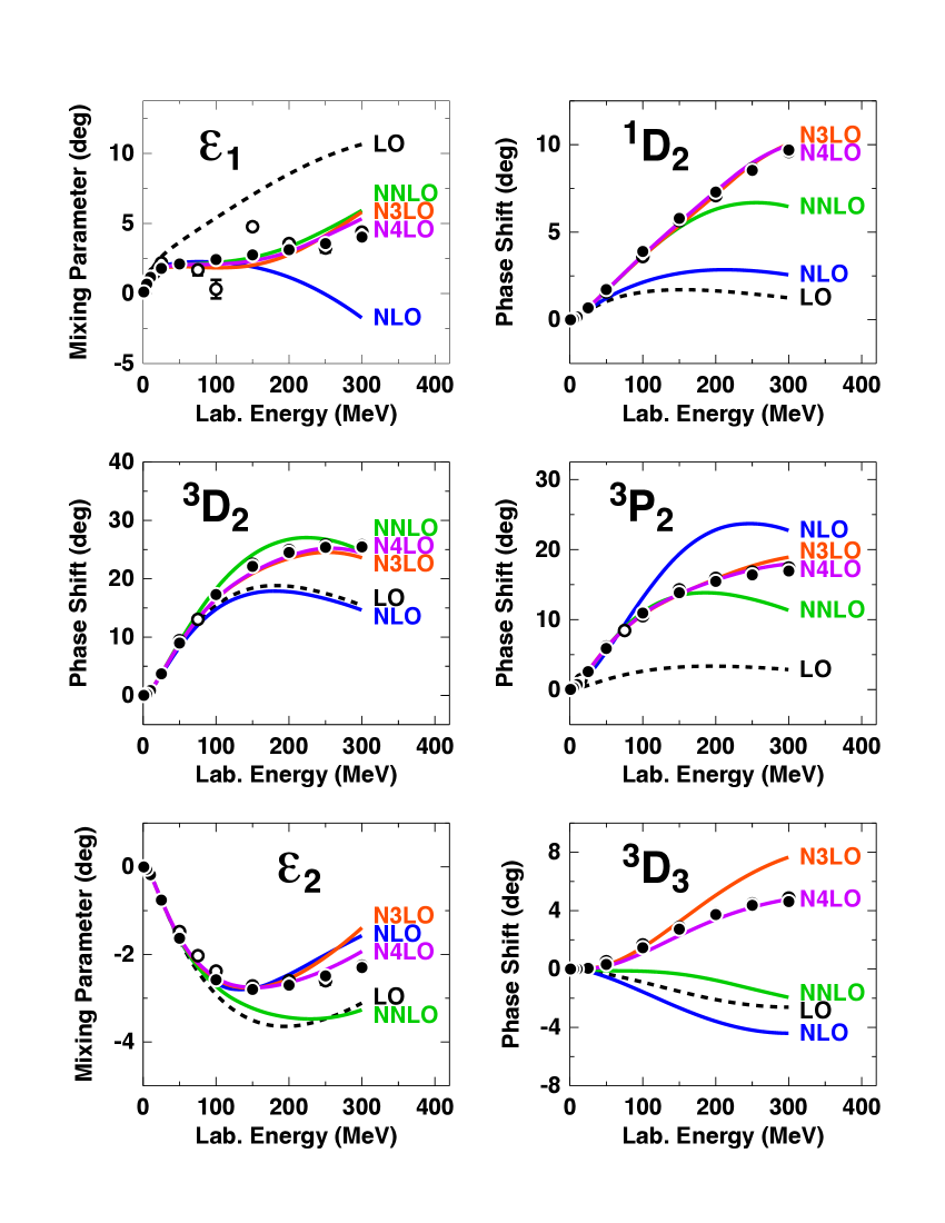
Figure 3.2: Chiral expansion of neutron-proton scattering as represented by the phase shifts in $S$, $P$, and $D$ waves and mixing parameters $\epsilon_{1}$ and $\epsilon_{2}$. Five orders ranging from LO to N⁴LO are shown as denoted ($\Lambda=500$ MeV in all cases). Filled and open circles as in Fig. 2.3. (From Ref. [94])

Table 3.2: $\chi^{2}/$datum for the fit of the 2016 $NN$ data base by $NN$ potentials at various orders of chiral EFT ($\Lambda=500$ MeV in all cases). (From Ref. [94])

$T_{\rm lab}$ bin (MeV)	No. of data	LO	NLO	NNLO	N3LO	N4LO
proton-proton
0–100	795	520	18.9	2.28	1.18	1.09
0–190	1206	430	43.6	4.64	1.69	1.12
0–290	2132	360	70.8	7.60	2.09	1.21
neutron-proton
0–100	1180	114	7.2	1.38	0.93	0.94
0–190	1697	96	23.1	2.29	1.10	1.06
0–290	2721	94	36.7	5.28	1.27	1.10
$pp$ plus $np$
0–100	1975	283	11.9	1.74	1.03	1.00
0–190	2903	235	31.6	3.27	1.35	1.08
0–290	4853	206	51.5	6.30	1.63	1.15

$NN$ potentials depend on two different sets of parameters, the $\pi N$ and the $NN$ LECs. The $\pi N$ LECs are the coefficients that appear in the $\pi N$ Langrangians. They are determined in $\pi N$ analysis [53], cf. Table 2.2. The $NN$ LECs are the coefficients of the $NN$ contact terms. They are fixed by an optimal fit to the $NN$ data below pion-production threshold, see Ref. [94] for details.

$NN$ potentials are then constructed order by order and the precision and accuracy improve as the order increases. How well the chiral expansion converges in important lower partial waves is demonstrated in Fig. 3.2, where we show phase parameters for potentials developed through all orders from LO to N⁴LO (of the $\Delta$-less theory). As a representative example, we show the predictions generated in Ref. [94], but for other families of recently constructed chiral $NN$ potentials [83, 87, 88, 91, 99], the picture is very similar. Fig. 3.2 clearly reveals substantial improvements in the reproduction of the empirical phase shifts with increasing order.

At this point, it is instructive to talk about the uncertainties of the phase shift predictions. As to be discussed in Sec. 5 below, the truncation error creates the largest uncertainty, for which the simplest formula is given by Eq. (5.1). Following this prescription, the error at a certain order is the difference between the given order and the next higher one. For example, the uncertainties of the NNLO phase shifts are given by the differences between the (green) NNLO curves and the (red) N3LO curves in Fig. 3.2. For the uncertainty at N4LO, Eq. (5.2) has to be invoked. The factor $Q$ in this formula is, of course, energy dependent but, as a simple rule of thumb, one may assume $Q\approx 1/3$.

The $\chi^{2}$/datum for the reproduction of the $NN$ data at various orders of chiral EFT are shown in Table 3.2 for different energy intervals below 290 MeV laboratory energy ($T_{\rm lab}$). The bottom line of Table 3.2 summarizes the essential results. For the nearly 5000 $pp$ plus $np$ data below 290 MeV (pion-production threshold), the $\chi^{2}$/datum is 51.4 at NLO and 6.3 at NNLO. Note that the number of $NN$ contact terms is the same for both orders. The improvement is entirely due to an improved description of the 2PE contribution, which is responsible for the crucial intermediate-range attraction of the nuclear force. At NLO, only the uncorrelated 2PE is taken into account which is insufficient. From the classic meson-theory of nuclear forces [14], it is wellknown that $\pi$-$\pi$ correlations and nucleon resonances need to be taken into account for a realistic model of 2PE. As discussed, in the chiral theory, these contributions are encoded in the subleading $\pi N$ vertexes. These enter at NNLO and are the reason for the substantial improvements we encounter at that order.

To continue on the bottom line of Table 3.2, after NNLO, the $\chi^{2}$/datum then further improves to 1.63 at N³LO and, finally, reaches the almost perfect value of 1.15 at N⁴LO—great convergence.

Table 3.3: Two- and three-nucleon bound-state properties as predicted by $NN$ potentials at various orders of chiral EFT ($\Lambda=500$ MeV in all cases). (Deuteron: Binding energy $B_{d}$, asymptotic $S$ state $A_{S}$, asymptotic $D/S$ state $\eta$, structure radius $r_{\rm str}$, quadrupole moment $Q$, $D$-state probability $P_{D}$; the predicted $r_{\rm str}$ and $Q$ are without meson-exchange current contributions and relativistic corrections. Triton: Binding energy $B_{t}$.) $B_{d}$ is fitted, all other quantities are predictions. (From Ref. [94])

	LO	NLO	NNLO	N3LO	N4LO	Empiricala
Deuteron
$B_{d}$ (MeV)	2.224575	2.224575	2.224575	2.224575	2.224575	2.224575(9)
$A_{S}$ (fm-1/2)	0.8526	0.8828	0.8844	0.8853	0.8852	0.8846(9)
$\eta$	0.0302	0.0262	0.0257	0.0257	0.0258	0.0256(4)
$r_{\rm str}$ (fm)	1.911	1.971	1.968	1.970	1.973	1.97507(78)
$Q$ (fm2)	0.310	0.273	0.273	0.271	0.273	0.2859(3)
$P_{D}$ (%)	7.29	3.40	4.49	4.15	4.10	—
Triton
$B_{t}$ (MeV)	11.09	8.31	8.21	8.09	8.08	8.48

^aSee Table XVIII of Ref. [12] for references; the empirical value for $r_{\rm str}$ is from Ref. [106].

The evolution of the deuteron properties from LO to N⁴LO of chiral EFT are shown in Table 3.3. In all cases, the deuteron binding energy is fit to its empirical value of 2.224575 MeV using the non-derivative ${}^{3}S_{1}$ contact. All other deuteron properties are predictions. Already at NNLO, the deuteron has converged to its empirical properties and stays there through the higher orders.

At the bottom of Table 3.3, we also show the predictions for the triton binding as obtained in 34-channel charge-dependent Faddeev calculations using only 2NFs. The results show smooth and steady convergence, order by order, towards a value around 8.1 MeV that is reached at the highest orders shown. This contribution from the 2NF will require only a moderate 3NF. The relatively low deuteron $D$-state probabilities ($\approx 4.1$% at N³LO and N⁴LO) and the concomitant generous triton binding energy predictions are a reflection of the fact that the $NN$ potentials are soft (which is, at least in part, due to the nonlocal character of these momentum-space potentials).

For a comparison with $\chi^{2}$ values from the older generation of high-precision potentials, the reader is referred to Ref. [107].

4   Nuclear many-body forces

Two-nucleon forces derived from chiral EFT have been applied, often successfully, in the many-body system. On the other hand, over the past several years we have learnt that, for some few-nucleon reactions and nuclear structure issues, 3NFs cannot be neglected. The most well-known cases are the so-called $A_{y}$ puzzle of $N$-$d$ scattering [108], the ground state of ¹⁰B [109], and the saturation of nuclear matter [110, 111, 112, 113, 114]. As we observed previously, the EFT approach generates consistent two- and many-nucleon forces in a natural way (cf. the overview given in Fig. 2.1). We now shift our focus to chiral three- and four-nucleon forces. For a recent review on this topic, see Ref. [115].

4.1   Three-nucleon forces

Weinberg [24] was the first to discuss nuclear three-body forces in the context of ChPT. Not long after that, the first 3NF at NNLO was derived by van Kolck [25].

For a 3NF, we have $A=3$ and $C=1$ and, thus, Eq. (2.5) implies

$$\nu=2+2L+\sum_{i}\Delta_{i}\,.$$ (4.1)

We will use this equation to analyze 3NF contributions order by order.

4.1.1   Next-to-leading order

The lowest possible power is obviously $\nu=2$ (NLO), which is obtained for no loops ($L=0$) and only leading vertices ($\sum_{i}\Delta_{i}=0$). As discussed by Weinberg [24] and van Kolck [25], the contributions from these diagrams vanish at NLO. So, the bottom line is that there is no genuine 3NF contribution at NLO—in the $\Delta$-less theory that we will mainly focus on when discussing many-body forces. For the modifications of the 3NFs when explicit $\Delta$ are introduced, see Fig. 2.5.

4.1.2   Next-to-next-to-leading order

The power $\nu=3$ (NNLO) is obtained when there are no loops ($L=0$) and $\sum_{i}\Delta_{i}=1$, i.e., $\Delta_{i}=1$ for one vertex while $\Delta_{i}=0$ for all other vertices. There are three topologies which fulfill this condition, known as the 2PE, 1PE, and contact graphs [25, 35] (Fig. 4.1).

The 2PE 3N-potential is derived to be

$$V^{\rm 3NF}_{\rm 2PE}=\left(\frac{g_{A}}{2f_{\pi}}\right)^{2}\frac{1}{2}\sum_{i\neq j\neq k}\frac{(\vec{\sigma}_{i}\cdot\vec{q}_{i})(\vec{\sigma}_{j}\cdot\vec{q}_{j})}{(q^{2}_{i}+m^{2}_{\pi})(q^{2}_{j}+m^{2}_{\pi})}\;F^{ab}_{ijk}\;\tau^{a}_{i}\tau^{b}_{j}$$ (4.2)

with $\vec{q}_{i}\equiv\vec{p_{i}}^{\prime}-\vec{p}_{i}$, where $\vec{p}_{i}$ and $\vec{p_{i}}^{\prime}$ are the initial and final momenta of nucleon $i$, respectively, and

$$F^{ab}_{ijk}=\delta^{ab}\left[-\frac{4c_{1}m^{2}_{\pi}}{f^{2}_{\pi}}+\frac{2c_{3}}{f^{2}_{\pi}}\;\vec{q}_{i}\cdot\vec{q}_{j}\right]+\frac{c_{4}}{f^{2}_{\pi}}\sum_{c}\epsilon^{abc}\;\tau^{c}_{k}\;\vec{\sigma}_{k}\cdot[\vec{q}_{i}\times\vec{q}_{j}]\;.$$ (4.3)

It is interesting to observe that there are clear analogies between this force and earlier 2PE 3NFs already proposed decades ago, particularly the Fujita-Miyazawa [116] and the Tucson-Melbourne (TM) [2] forces. In fact, based upon the chiral 3NF at NNLO, the TM force was corrected [117] leading to what became known as the TM’ or TM99 force [3].

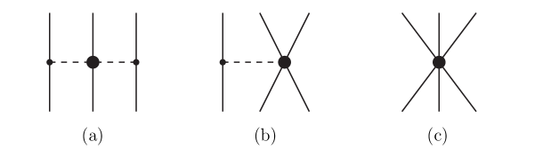
Figure 4.1: The three-nucleon force at NNLO with (a) 2PE, (b) 1PE, and (c) contact diagrams. Notation as in Fig. 2.1.

The 2PE 3NF does not introduce additional fitting constants, since the LECs $c_{1,3,4}$ are fixed in $\pi N$ analysis (cf. Table 2.2) and are already present in the 2PE 2NF.

The other two 3NF contributions shown in Fig. 4.1 are the 1PE contribution

$$V^{\rm 3NF}_{\rm 1PE}=-\frac{c_{D}\,g_{A}}{8f^{4}_{\pi}\,\Lambda_{\chi}}\sum_{i\neq j\neq k}\frac{\vec{\sigma}_{j}\cdot\vec{q}_{j}}{q^{2}_{j}+m^{2}_{\pi}}(\mbox{\boldmath$\tau$}_{i}\cdot\mbox{\boldmath$\tau$}_{j})(\vec{\sigma}_{i}\cdot\vec{q}_{j})$$ (4.4)

and the 3N contact potential

$$V^{\rm 3NF}_{\rm ct}=\frac{c_{E}}{2f_{\pi}^{4}\,\Lambda_{\chi}}\sum_{i\neq j\neq k}\mbox{\boldmath$\tau$}_{i}\cdot\mbox{\boldmath$\tau$}_{j}$$ (4.5)

with $\Lambda_{\chi}=700$ MeV. These 3NF potentials introduce two additional constants, $c_{D}$ and $c_{E}$, which can be constrained in more than one way. One may use the triton binding energy and the $nd$ doublet scattering length ${}^{2}a_{nd}$ [35] or an optimal global fit of the properties of light nuclei [118]. Alternative choices include the binding energies of ³H and ⁴He [119] or the binding energy of ³H and the point charge radius of ⁴He [120]. Another method makes use of the triton binding energy and the Gamow-Teller matrix element of tritium $\beta$-decay [121]. When the values of $c_{D}$ and $c_{E}$ are fixeded, the results for other observables involving three or more nucleons are true theoretical predictions.

A comprehensive study of all possible operator structures that enter the leading and subleading contact 3NF can be found in Ref. [45]. In Ref. [103], the NM EoS was calculated with different choices of the 3NF contact operator and found to be consistent with other ab initio determinations within uncertainties.

Applications of the leading 3NF include few-nucleon reactions [35, 122, 123], structure of light- and medium-mass nuclei [124, 125, 126, 127, 128, 129, 130, 131, 132, 133, 134, 135, 136, 137], and infinite matter [110, 111, 112, 113, 114, 120, 138, 139, 140]. One of the greatest successes of the NNLO 3NF is that it solves the problem of the saturation of nuclear matter [110, 111, 112]—a problem that has a long history.

Originally, it was hoped that nuclear matter saturation and the structure of finite nuclei could be understood in terms of just the 2NF [141]—if one would only find the “right” 2NF. However, in the course of the 1970’s, when more reliable microscopic calculations became available, growing evidence accumulated that showed that it was impossible to saturate nuclear matter at the right energy and density when applying only 2NFs [142, 143, 11]. Another problem was the triton binding energy, which was considerably underpredicted with the 2NFs available at the time [144, 145]. These failures were interpreted as an indication for the need of nuclear many-body forces.

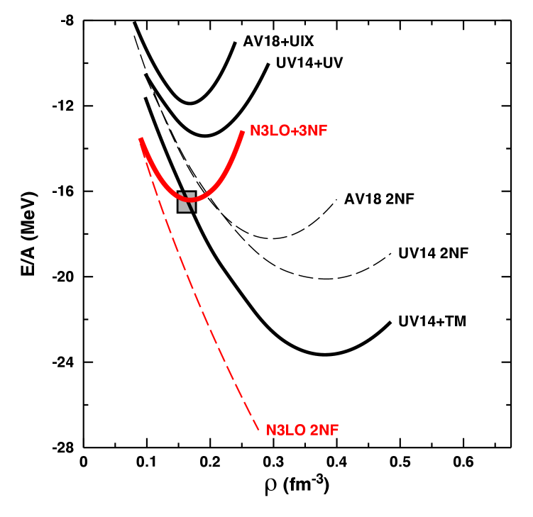
Figure 4.2: Energy per nucleon, $E/A$, as a function of density, $\rho$, of symmetric nuclear matter (SNM). Black dashed curves represent predictions applying purely phenomenologial 2NFs with UV14 referring to the Urbana $v_{14}$ 2NF [4] and AV18 signifying the Argonne $v_{18}$ 2NF [1]. Solid black curves include phenomenological 3NFs with TM denoting the Tucson-Melbourne [2], UV the Urbana V [5], and UIX the Urbana IX [6] 3NF models. Red curves depict results from chiral EFT based forces [94, 114]. The shaded box marks the area in which empirical nuclear matter saturation is presumed to occur.

Thus, in the late 1970’s and early 1980’s, various phenomenological 3NFs were constructed, like the TM [2] and the Urbana [5] forces. The attraction provided by the TM 2PE 3NFs has proven to be useful in explaining the binding energies of light nuclei (particularly, ³H and ⁴He) which are, in general, underbound when only 2NFs are applied. However, this added attraction leads to overbinding and too high a saturation density in nuclear matter (cf. Fig. 4.2, curve labeled UV14+TM). Therefore, some groups added a repulsive short-range 3NF which ameliorates the problem, but does not solve it [143, 5] (Fig. 4.2, curve UV14+UV). In the work by the Urbana group, many versions of such 3NF were developed with Urbana IX (UIX) being the most popular one (Fig. 4.2, curve AV18+UIX). In later work [63], the Urbana group extended their model for the 3NF by including the $2\pi$-exchange $S$-wave contribution plus three-pion exchange ring diagrams with one $\Delta$ excitation. The peculiar spin and isospin dependencies of $\Delta$-ring diagrams were found to be helpful in the explanation of spectra of light nuclei. This has become known as the Illinois 3NFs [63], which so far have evolved up to Illinois-7 (IL7) [146].

The 3NFs of the Urbana type, adjusted to the ground state and the spectra of light nuclei, do not saturate nuclear matter properly [5, 147] (Fig. 4.2, curves UV14+UV and AV18+UIX) and severely underbind intermediate-mass nuclei [148]. The AV18 2NF plus IL7 3NF yield a pathological equation of state of pure NM [149]. In addition, the so-called $A_{y}$ puzzle of nucleon-deuteron scattering [108] is not resolved by any of the phenomenological 3NFs [150].

In view of this long and desperate history of failed attempts to solve the nuclear matter problem, the success of the the chiral NNLO 3NF is outstanding, see red ‘N3LO+3NF’ curve in Fig. 4.2.

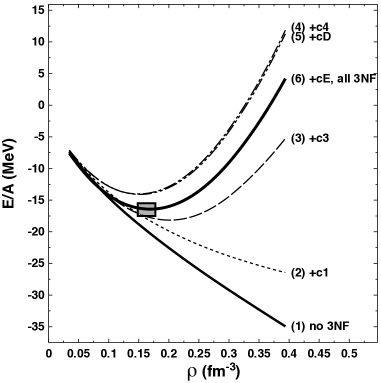
Figure 4.3: Energy per nucleon, $E/A$, as a function of density, $\rho$, of SNM from the chiral EFT based interaction. Curve (1) shows the result when only the 2NF is used. Curve (6) displays the final result after all (NNLO) 3NF contributions have been added. The individual 3NF contributions are added up successively in the order given by the parenthetical numbers. The LECs $c_{1,3,4}$ parametrize the 2PE 3NF, while $c_{D}$ and $c_{E}$ are the coefficients of the 1PE and contact 3NF diagrams, respectively.

It it interesting to dissect how the chiral 3NF achieves saturation. For this purpose, we display in Fig. 4.3 the effects of the individual chiral NNLO 3NF terms. Curves (2) to (4) show the impact of the 2PE 3NF [Fig. 4.1(a)], while curves (5) and (6) exhibit the contributions from the 3NF diagrams Fig. 4.1(b) and (c), respectively. Obviously, the 2PE 3NF component does the job, namely, provides a strongly density-dependent repulsive force that generates saturation at the right energy and density.

In summary, the leading (NNLO) 3NF of ChPT is a remarkable contribution. It gives validation to, and provides a better framework for, 3NFs which were proposed already five decades ago; it alleviates existing problems in few-nucleon reactions and the spectra of light nuclei and, particularly, solves the nuclear matter problem.

Some problems, though, remain unresolved at this order (NNLO), such as the well-known ‘$A_{y}$ puzzle’ in nucleon-deuteron scattering [108, 35] which, however, will be solved by the 3NF at N⁴LO, see below.

As discussed earlier, for the 2NF, it turned out to be necessary to go to order four or even five for convergence and high-precision predictions. Thus, the 3NF at N³LO and N⁴LO must be considered simply as a matter of consistency with the 2NF sector. At the same time, one hopes that its inclusion may result in improvements with the still unresolved problems.

4.1.3   Next-to-next-to-next-to-leading order

At N³LO, there are loop and tree diagrams. For the loops (Fig. 4.4), we have $L=1$ and, therefore, all $\Delta_{i}$ have to be zero to ensure $\nu=4$. Thus, these one-loop 3NF diagrams can include only leading order vertices, the parameters of which are fixed from $\pi N$ and $NN$ analysis. The diagrams have been evaluated by the Bochum-Bonn group [39, 40]. The long-range part of the chiral N³LO 3NF has been tested in the triton and in three-nucleon scattering [151] leaving the $N-d$ $A_{y}$ puzzle unresolved. The long- and short-range parts of this force have been applied in calculations of both SNM and NM [152, 153, 154, 155, 156] as well as in the structure of medium-mass nuclei [157, 158] with, partially, great success.

Figure 4.4: Leading one-loop 3NF diagrams at N³LO. We show one representative example for each of five topologies, which are: (a) 2PE, (b) 1PE-2PE, (c) ring, (d) contact-1PE, (e) contact-2PE. Notation as in Fig. 2.1.

4.1.4   The 3NF at N⁴LO

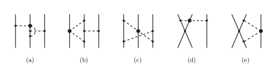
Figure 4.5: Sub-leading one-loop 3NF diagrams which appear at N⁴LO with topologies similar to Fig. 4.4. Notation as in Fig. 2.1.

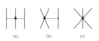
Figure 4.6: 3NF tree graphs at N⁴LO ($\nu=5$) denoted by: (a) 2PE, (b) 1PE-contact, and (c) contact. Notation as in Fig. 2.1.

In regard to some unresolved issues, one may go ahead and look at the next order of 3NFs, which is N⁴LO or $\nu=5$. The loop contributions that occur at this order are obtained by replacing in the N³LO loops one vertex by a $\Delta_{i}=1$ vertex (with LEC $c_{i}$), Fig. 4.5, which is why these loops may be more sizable than the N³LO loops. The 2PE, 1PE-2PE, and ring topologies have been evaluated [30, 43] so far. In addition, we have three ‘tree’ topologies (Fig. 4.6), which include a new set of 3N contact interactions that has been derived by the Pisa group [44]. The N⁴LO 3NF contacts have been applied with success in calculations of few-body reactions at low energy solving the $p$-$d$ $A_{y}$ puzzle [45], Fig. 4.7. This is an outstanding success in view of the $A_{y}$ puzzle’s long history [108].

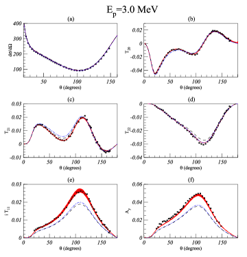
Figure 4.7: Cross section and polarization observables of $p$-$d$ scattering at 3 MeV proton energy as predicted by the AV18 2NF [1] (black dashed lines), the AV18 2NF + UIX 3NF [6] (blue dash-dotted lines), and calculations that include chiral N⁴LO 3NF contact terms [45] (red bands). The width of the red bands reflect the uncertainty when the cutoff varies between $\Lambda$=200 MeV and 500 MeV. Data from Ref. [159]. (Figure reproduced from Ref. [45] with permission.)

4.2   Four-nucleon forces

For connected ($C=1$) $A=4$ diagrams, Eq. (2.5) yields

$$\nu=4+2L+\sum_{i}\Delta_{i}\,.$$ (4.6)

We then see that the first (connected) non-vanishing 4NF is generated at $\nu=4$ (N³LO), with all vertices of leading type, Fig. 4.8. This 4NF has no loops and introduces no novel parameters [41].

For a reasonably convergent series, terms of order $(p/\Lambda_{b})^{4}$ should be small and, therefore, chiral 4NF contributions are expected to be very weak. This has been confirmed in calculations of the energy of ⁴He [160] as well as NM and SNM [152].

The effects of the leading chiral 4NF in SNM and pure NM have been worked out by Kaiser et al. [161, 162].

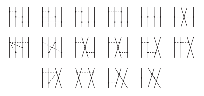
Figure 4.8: Leading four-nucleon force at N³LO.

5   Uncertainty quantification

When applying chiral two- and many-body forces in ab initio calculations producing predictions for observables of nuclear structure and reactions, major sources of uncertainties are [163]:

1. Experimental errors of the input $NN$ data that the 2NFs are based upon and the input few-nucleon data to which the 3NFs are adjusted.

2. Uncertainties in the Hamiltonian due to

   1. uncertainties in the determination of the $NN$ and $3N$ contact LECs,

   2. uncertainties in the $\pi N$ LECs,

   3. regulator dependence,

   4. EFT truncation error.

3. Uncertainties associated with the few- and many-body methods applied.

1. Experimental errors of the input $NN$ data that the 2NFs are based upon and the input few-nucleon data to which the 3NFs are adjusted.
   In Ref. [164], the authors systematically investigated this error propagation by constructing a family of smooth local potentials the parameters of which carry the uncertainties implied by the errors in the $NN$ data. With 205 Monte Carlo samples of these potentials, they found an uncertainty of 15 keV for the triton binding energy. In a more recent study [165] that used 33 Monte Carlo samples, the uncertainty of 15 keV for the triton binding energy was reproduced, and the uncertainty for the ⁴He binding energy was detrmined to be 55 keV. Our assessment is that statistical error propagation from the $NN$ input data is negligible as compared to uncertainties from other sources discussed below.
   Regarding the propagation of experimental errors from the few-nucleon data used to fit the 3NF contact terms, this uncertainty can be made very small by adjusting the 3NFs to data with very small experimental errors; for instance, the measured binding energy of the triton is 8.481795 $\pm$ 0.000002 MeV, which will lead to negligible propagation.

2. Uncertainties in the Hamiltonian due to

   1. uncertainties in the determination of the $NN$ and $3N$ contact LECs.
      We have fitted the $NN$ contact LECs to the $NN$ data below 100 MeV at LO and NLO, below 190 MeV at NNLO, and below 290 MeV at N3LO and N4LO. Based on our experience [96], we do not expect significant errors from variations of the fit intervals at the low energies appropriate for chiral EFT.
      As for the contact 3NF LECs, they can be fixed through a number of different procedures, that is, fitting different observables. For observables that were not part of the fitting protocol, predictions obtained with LECs from different methods will be different, and such differences can be taken as a measure of the uncertainty from this source.

   2. Uncertainties in the $\pi N$ LECs.
      Since the high-precision determination of the $\pi N$ LECs from Roy-Steiner analyses [52, 53], this uncertainty can essentially be ignored.

   3. Regulator dependence, see discussion below.

   4. EFT truncation error, see discussion below.

3. Uncertainties associated with the few- and many-body methods applied.
   This is unrelated to chiral EFT. While few-body systems can be solved exactly, predictions for heavier nuclei and nuclear matter will carry this uncertainty regardless the chosen method. Many-body theory practitioners may probe the size of this uncertainty by comparing their predicted observable with predictions from different many-body methods and otherwise identical input, if available.

The choice of the regulator function and its cutoff parameter creates uncertainty. Originally, cutoff variations were perceived as a demonstration of the uncertainty at a given order (equivalent to the truncation error). However, in various investigations [112, 83] it has been shown that this is not correct and that cutoff variations, in general, underestimate this uncertainty. Therefore, the truncation error is better determined by sticking literally to what ‘truncation error’ means, namely, the error due to ignoring contributions from orders beyond the given order $\nu$. The largest such contribution is the one of order $(\nu+1)$, which one may, therefore, consider as representative for the magnitude of what is left out.

This suggests that the truncation error at order $\nu$ can reasonably be estimated as

$$\Delta X_{\nu}(p)=|X_{\nu}(p)-X_{\nu+1}(p)|\,,$$ (5.1)

where $X_{\nu}(p)$ denotes the prediction for observable $X$ at order $\nu$ and momentum $p$. If $X_{\nu+1}$ is not available, then one may use,

$$\Delta X_{\nu}(p)=|X_{\nu-1}(p)-X_{\nu}(p)|Q\,,$$ (5.2)

with the expansion parameter $Q$ chosen as

$$Q=\max\left\{\frac{m_{\pi}}{\Lambda_{b}},\;\frac{p}{\Lambda_{b}}\right\}\,,$$ (5.3)

where $p$ is the characteristic center-of-mass (CMS) momentum scale and $\Lambda_{b}$ the breakdown scale.

Alternatively, one may also apply the more elaborate scheme suggested in Ref. [83] where the truncation error at, e.g., N³LO is calculated in the following way:

$$\Delta X_{\rm N^{3}LO}(p) = \max\left\{Q^{5}\times\left|X_{\rm LO}(p)\right|,\;\;Q^{3}\times\left|X_{\rm LO}(p)-X_{\rm NLO}(p)\right|,\;\;Q^{2}\times\left|X_{\rm NLO}(p)-X_{\rm NNLO}(p)\right|,\;\;\right.$$ (5.5)

$$\left.Q\times\left|X_{\rm NNLO}(p)-X_{\rm N^{3}LO}(p)\right|\right\}\,,$$

with $X_{\rm N^{3}LO}(p)$ denoting the N³LO prediction for observable $X(p)$, etc.. This more sophisticated formula is especially useful, whenever—by accident—the difference between the highest two orders is uncharacteristically small. “Extrapolating” the errors of the lower orders may then provide a more realistic estimate.

Note that one should not add up (in quadrature) the uncertainties due to regulator dependence and the truncation error, because they are not independent. In fact, it is appropriate to leave out the uncertainty due to regulator dependence entirely and just focus on the truncation error [83]. The latter should be estimated using the same cutoff in all orders considered. In summary, the truncation error is the dominant source of (systematic) error that can be reliably estimated in the EFT approach.

The above is not a comprehensive statistical analysis. Statistically robust Bayesian methods have been developed and applied, see, for instance, Ref. [166]. The BUQEYE collaboration (Bayesian Uncertainty Quantification: Errors in Your EFT) works with projection-based, reduced-order emulators for applications in low-energy nuclear physics [167].

6   Applications in the nuclear many-body problem

Table 6.1: Microscopic calculations of finite nuclei and nucleonic matter applying chiral forces published during the past decade (see Table  1.1 for abbreviations and acronyms used).

Year	Authors/collab.	2NF	3NF	$\Delta$sc	Nuclear systems(s)	Many-body method(s)	Ref(s).
	.	Order (cutoffa) localityb	Order (cutoffa) localityb
Set 1: Momentum space, nucleonic matter:
2013	Tews et al.	N3LO (450, 500) nl	N3LO (450, 500) nl + 4NF	No	NM	MBPT	[168]
2013	Coraggio et al.	N3LO (414-500) nl	NNLO (414, 500) nl	No	NM	MBPT	[140]
2014	Coraggio et al.	N3LO (414-500) nl	NNLO (414, 500) nl	No	SNM	MBPT	[111]
2014	Hagen et al.	NNLO (500) nl	NNLO (400, 500) loc, nl	No	SNM, NM	BHF	[139]
2015	Sammarruca et al.	NNLO, N3LO (450-600) nl	NNLO (450-600) nl	No	SNM, NM	BHF	[112]
2019	Drischler et al.	NNLO, N3LO (450, 500) nl	NNLO, N3LO (450, 500) nl	No	SNM, NM	MBPT	[155]
2020	Drischler et al.	LO-N3LO (450, 500) nl	NNLO, N3LO (450, 500) nl	No	NM	MBPT	[169]
2021	Sammarruca et al.	LO-N3LO (450) nl	NNLO-N3LO (450) nl	No	NM	BHF	[170]
2021	Sammarruca et al.	LO-N3LO (450) nl	NNLO-N3LO (450) nl	No	SNM	BHF	[171]
2021	Keller et al.	NNLO, N3LO (450, 500) nl	NNLO, N3LO (450, 500) nl	No	NM	MBPT	[172]
2023	Keller et al.	NNLO, N3LO (450, 500) nl	NNLO, N3LO (450, 500) nl	No	ASNM	MBPT	[173]
Set 2: Momentum space, finite nuclei (and nucleonic matter):
2013	Ekström et al.	NNLO (500) nl	NNLO (500) nl	No	10Be - 56Ca, NM	NCSM, CC	[85]
2013	Hergert et al.	N3LO (500) nl	NNLO (400) loc	No	4He - 56Ni	IM-SRG	[130]
2014	Binder et al.	N3LO (500) nl	NNLO (350, 400) loc	No	16O - 132Sn	SRG, CC	[132]
2015	Ekström et al.	NNLO (450) nl	NNLO (450) nl	No	4He - 40Ca, SNM	CC	[92]
2017	Stroberg et al.	N3LO (500) nl	NNLO (400) loc	No	C - Ni	IM-SRG	[174]
2017	Simonis et al.	N3LO (1.8, RG evolved) nl	NNLO (2.0) nl	No	4He - 78Ni	IM-SRG	[135]
2018	Morris et al.	N3LO (1.8, RG evolved) nl	NNLO (2.0) nl	No	100-111Sn, 105Te	IM-SRG	[136]
2018	Ekström et al.	NNLO (450, 500) nl	NNLO (450, 500) nl	Yes	4He - 48Ca, SNM, NM	CC	[93]
2019	Hoppe et al.	NLO-N3LO (420-500) nl	NNLO-N3LO (420-500) nl	No	4He - 68Ni	IM-SRG	[157]
2020	Huether et al.	NLO-N3LO (450-550) nl	NNLO-N3LO (450-550) nl	No	16O - 78Ni	IM-SRG	[158]
2020	Soma et al.	N3LO (500) nl	NNLO (500/650) lnl	No	Li - Ni	NCSM, ADC(3)	[137]
2020	Jiang et al.	NNLO (394, 450) nl	NNLO (394, 450) nl	Yes	4He - 132Sn, SNM, NM	CC	[98]
2022	Miyagi et al.	N3LO (1.8, RG evolved) nl	NNLO (2.0) nl	No	132Sn, 127Cd	HF-MBPT, IM-SRG	[175]
2022	LENPIC	LO-N4LO+ (400-550) nl	NNLO (400-550) nl	No	3H - 48Ca	NCCI, IM-SRG	[176]
Set 3: Configuration space calculations:
2014	Gezerlis et al.	LO-NNLO (1.0-1.2) loc	None	No	NM	AFDMC, MBPT	[86]
2016	Tews et al.	LO-NNLO (1.0-1.2) loc	NNLO (1.0-1.2) loc	No	NM	AFDMC	[177]
2016	Lynn et al.	NLO-NNLO (1.0-1.2) loc	NNLO (1.0-1.2) loc	No	3H-4He, NM	GFMC	[178, 179]
2016	Piarulli et al.	LO-N(3)LOd (0.8-1.2) loc	None	Yes	3H-6Li	HH, GFMC	[88]
2018	Piarulli et al.	N(3)LOd (1.0-1.2) loc	NNLO (1.0-1.2) loc	Yes	3H-12C	HH, GFMC	[180]
2018	Lonardoni et al.	LO-NNLO (1.0-1.2) loc	NNLO (1.0-1.2) loc	No	3H-16O	AFDMC, GFMC	[181]
2018	Tews et al.	LO-NNLO (1.0) loc	NNLO (1.0) loc	No	NM	AFDMC	[182]
2020	Lonardoni et al.	NNLO (1.0) loc	NNLO (1.0) loc	No	SNM, NM	AFDMC	[183]
2022	Lovato et al.	N(3)LOd (1.0, 1.2) loc	NNLO (1.0, 1.2) loc	Yes	NM	BHF, FHNC, AFDMC	[184]

^a Cutoff numbers above 100 are in units of MeV, below 100 in units of fm.
^b loc = local, nl = nonlocal, lnl = local/nonlocal.
^c $\Delta(1232)$-isobar excitations included, yes or no?
^d 2PE at NNLO, contacts at N³LO.

6.1   The ab initio approach to finite nuclei

The tenet of microscopic nuclear theory is that atomic nuclei can be accurately described as collections of point-like nucleons interacting via two- and many-body forces obeying nonrelativistic quantum mechanics—the forces being fixed in free-space scattering. The microscopic or ab initio approach to nuclear structure and reactions is then defined as calculating the properties of nuclei in accordance with the tenet. Before we will report on the latest calculations of this kind, we will briefly review the history of this approach, because some mistakes of history are being repeated today.

6.1.1   Historical perspective

The microscopic approach to nuclear structure is almost as old as nuclear physics itself. Brueckner and co-workers introduced Brueckner theory as early as 1954 [185] and performed the first semi-realistic microscopic nuclear matter calculation in 1958 [186]. Already that same year, Brueckner discussed finite nuclei proposing the local density approximation [187].

In the second half of the 1960’s, one of the hottest topics in nuclear structure physics was calculating the properties of finite nuclei without recourse through nuclear matter using Brueckner-Hartree-Fock (BHF) theory. The Oak Ridge National Laboratory (ORNL) with its computer power played a leading role in this effort that was guided by Thomas Davies and Michel Baranger [188, 189]. BHF (and coupled cluster) calculations of finite nuclei continued into the early 1970s with work by the Bochum [190] and the Bonn-Jülich groups [191].

In parallel to the above developments, research on the microscopic derivation of the shell-model effective interaction was conducted (again, applying Brueckner theory) that had been kicked off by Kuo and Brown in 1966 [192].

Applying the nucleon-nucleon ($NN$) potentials available at the time, the BHF approach reproduced about one half of the binding energies of closed-shell nuclei which, in the early phase, was seen as a great success [188], but in the long run did not satisfy demands for more quantitative predictions. Therefore, a departure from the microscopic approach happened around 1973 as reflected most notably in a lead-talk by Michel Baranger at the International Conference on Nuclear Physics in Munich in 1973 [193].

The shell-model effective interaction suffered a similar fate at the International Conference on Effective Interactions and Operators in Nuclei in Tucson, Arizona, in 1975, organized by Bruce Barrett [194].

And so it happened that in the early 1970s, the microscopic approach was abandoned and replaced by phenomenological effective interactions (also know as mean-field models): the Skyme interaction [195] as revived by Vautherin and co-workers [196, 197], the Gogny force [198, 199], and the relativistic mean-field model of Walecka [200, 201].

Ironically, the calculations with those effective interactions continued to be called “microscopic”, for which John Negele had provided the (debatable) justification in his Ph.D.  thesis of 1970 [141]. Before calculating finite nuclei in the local density approximation, Negele had adjusted the insufficient binding of nuclear matter provided by the Reid soft-core potential [202] (11 MeV per nucleon) by hand to the presumed empirical value of 15.68 MeV making “the assumption that when higher-order corrections have been evaluated carefully, nuclear-matter theory will indeed produce the correct binding” [141]. Negele had many followers [203, 204, 205].

However, the true “deeper reason” for those effective interactions was much simpler: “To get better results!” [206]. Clearly, the trends that won popularity in the early 1970s were a setback for the fundamental research in nuclear structure.

Nuclear structure theory at its basic level is not about fitting data to get “good” results. Fundamental nuclear structure theory is about answering the question:

Do the same nuclear forces that explain free-space scattering experiments also explain the properties of finite nuclei and nuclear matter when applied in nuclear many-body theory?

One can think of many reasons why the basic tenet should be wrong. According to the EMC effect, nucleons swell when inserted into nuclei which might affect the force between nucleons [207]. Meson exchange in the nuclear medium may be different than in free-space for various reasons [208, 209, 210]. The excitation of resonances, e. g. $\Delta(1232)$ isobars, within the nucleon-nucleon interaction process is subject to changes when happening in a nuclear medium [211, 212, 213, 55]. And many more ideas have been advanced, like e. g., Brown-Rho scaling [214]. In fact, in the 1970s, a popular belief was that medium effects on the $NN$ interaction may be the solution to the problem of lacking saturation [11].

Thus, it is a good question to ask whether medium modifications of nuclear forces show up in a noticeable way and/or are even needed for quantitative nuclear structure predictions. But when we re-adjust the free-space forces arbitrarily to get “good” results, then we will never find out. Note also that at some (high) energy and high density, the picture of point-like nucleons is bound to break down [215]. So, the issue behind the nuclear theory tenet is: Are the energies typically involved in conventional nuclear structure physics low enough to treat nucleons as structure-less objects?

To come back to history: the renunciation of the truly microscopic approach lasted about two decades (essentially the 1970s and 80s). Then, in the early 1990s, the microscopic theory was revived by the Argonne-Urbana group [216, 6]. The crucial element in those new microscopic calculations was the inclusion of a three-nucleon force (3NF). The idea of a nuclear 3NF was not new. In fact, it is almost as old as meson theory itself [217]. But for years it had been considered just an academic topic, too difficult to incorporate into actual calculations, anyhow. But the persistent failure to saturate nuclear matter at reasonable energies and densities, as well as the the underbinding of nuclei, finally compelled nuclear structure physicists to take a serious look at the 3NF issue, as explained in the exemplary Comment by Ben Day [143] based upon first test calculations by the Urbana group [5]. The 3NF definitely improved nuclear saturation and the properties of light nuclei, even though nothing was perfect [6] (cf. Fig. 4.2).

6.1.2   Recent advances

After the year of 2000, two changes occurred. First, the term ‘microscopic’ was increasingly replaced by the term ‘ab initio’ [218]—for reasons nobody knows (but nothing to worry about because both mean the same). Second and more importantly, nuclear forces based upon chiral effective field theory (EFT) entered the picture [81, 38]. This development was of great advantage. Note that for a microscopic approach to be truly microscopic, the free-space forces need to be accurate. But with phenomenological or meson-theoretic forces it was difficult to define what sufficiently accurate means, since the errors in those theories are unknown. However, in the framework of an EFT, the theoretical uncertainty can be determined (cf. Sec. 5) and, thus, related with the accuracy of the predictions. Hence, in the framework of an EFT:

Accurate free-space forces are forces that predict experiment within the theoretical uncertainty of the EFT at the given order.

After 2000, it also became well established that predictive nuclear structure must include 3NFs, besides the usual two-nucleon force (2NF) contribution. Another advantage of chiral EFT is then that it generates 2NFs and multi-nucleon forces simultaneously and on an equal footing. In the $\Delta$-less theory [26, 27], 3NFs occur for the first time at next-to-next-to-leading order (NNLO) and continue to have additional contributions in higher orders. If an explicit $\Delta$-isobar is included in chiral EFT ($\Delta$-full theory [23, 58, 59, 60]), then 3NF contributions start already at next-to-leading order (NLO).

In the initial phase, the 3NFs were typically adjusted in $A=3$ and/or the $A=4$ systems and the ab initio calculations were driven up to the oxygen region [129]. It turned out that for $A\raisebox{-1.29167pt}{\small$\ \stackrel{{\scriptstyle\textstyle<}}{{\sim}}$ }16$ the ground-state energies and radii are predicted about right, no matter what type of chiral or phenomenological potentials were applied (local, nonlocal, soft, hard, etc.) and what the details of the 3NF adjustments to few-body systems were [129, 125, 180, 181, 219, 176].

However, around the year of 2015, the picture changed, when the many-body practitioners were able to move up to medium-mass nuclei (e. g., the calcium or even the tin regions). Large variations of the predictions now occurred depending on what forces were used, and cases of severe underbinding [148] as well as of substantial overbinding [132] were observed. Ever since, the nuclear structure community understands that accurate ab initio explanations of intermediate and heavy nuclei is an outstanding problem.

There have been several attempts to predict the properties of medium-mass nuclei with more accuracy. Of the various efforts, we will now list four cases, which are representative for the status, and will denote each case with a short label for ease of communication. We restrict ourselves to cases, where the properties of medium-mass nuclei and nuclear matter have been calculated, because the simultaneous description of both systems is part of the problem.

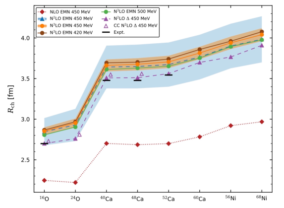
Figure 6.1: Upper panel: Ground-state energies per nucleon, $E/A$, of selected closed-shell oxygen, calcium, and nickel isotopes as obtained in the “Hoppe” case [157]. Results are shown for various chiral interactions as denoted. The blue and orange bands give the NNLO and N³LO uncertainty estimates, respectively. $\Lambda=450$ MeV in all cases except the green curve. Black bars indicate experimental data. Lower panel: Same as upper panel, but for charge radii. (Reproduced from Ref. [157] with permission.)

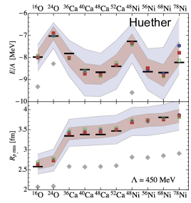
Figure 6.2: Ground-state energies per nucleon (top panel) and point-proton rms radii (bottom panel) for selected medium-mass isotopes as obtained in the “Hüther” case [158]. The light blue and pink bands represent the theoretical uncertainties at NNLO and N³LO, respectively. $\Lambda=450$ MeV. Black bars indicate the experimental data. (Figure courtesy of R. Roth)

• “Magic” [120, 115]: A seemingly successful interaction for the intermediate mass region commonly denoted by “1.8/2.0(EM)” (sometimes dubbed “the Magic force”). It is a similarity renormalization group (SRG) evolved version of the N³LO 2NF of Ref. [38] complemented by a NNLO 3NF adjusted to the triton binding energy and the point charge radius of ⁴He. With this force, the ground-state energies all the way up to the tin isotopes are reproduced perfectly—but with charge radii being on the smaller side [135, 136]. Nuclear matter saturation is also reproduced reasonably well, but at a slightly too high saturation density [120].

• “GO” [93, 98]: A family of $\Delta$-full NNLO potentials constructed by the Göteborg/Oak Ridge (GO) group. The authors claim to obtain “accurate binding energies and radii for a range of nuclei from $A=16$ to $A=132$, and provide accurate equations of state for nuclear matter” [98].

• “Hoppe” [155, 157]: Recently developed soft chiral 2NFs [94] at NNLO and N³LO complemented with 3NFs at NNLO and N³LO, respectively, to fit the triton binding energy and nuclear matter saturation. These forces applied in in-medium similarity renormalization group (IM-SRG [220]) calculations of finite nuclei up to ⁶⁸Ni predict underbinding and slightly too large radii [157], see Fig. 6.1.

• “Hüther” [158]: The same 2NFs used in “Hoppe”, but with the 3NFs adjusted to the triton and ¹⁶O ground-state energies. The interactions so obtained reproduce accurately experimental energies and point-proton radii of nuclei up to ⁷⁸Ni [158], see Fig. 6.2. However, when the 2NF plus 3NF combinations of “Hüther” are utilized in nuclear matter, then overbinding and no saturation at realistic densities is obtained [156], see Fig. 6.3.

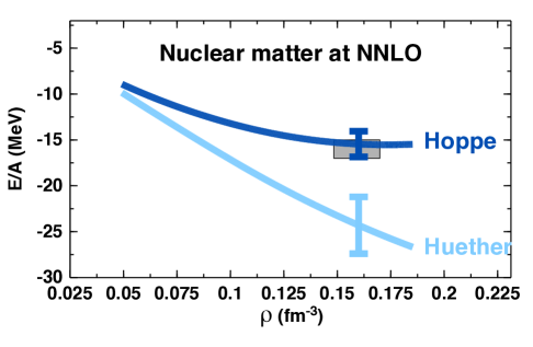
Figure 6.3: Energy per nucleon, $E/A$, as a function of density, $\rho$, of SNM as obtained in calculations with the 2NFs and 3NFs consistently at NNLO [156]. In the two cases shown, the 2NF is the same, while the 3NFs are the ones used in the calculations of finite nuclei in the “Hoppe” and “Huether” cases as denoted. $\Lambda=450$ MeV in both cases. The error bars show the theoretical uncertainties around saturation, which is expected to occur in the area of the gray box.

Obviously, in some cases, there appears to be a problem with achieving simultaneously accurate results for nuclear matter and medium-mass nuclei: In the “Hoppe” case, nuclear matter is saturated correctly, but nuclei are underbound; while in the “Hüther” case, nuclei are bound accurately, but nuclear matter is overbound. Other cases seem to have solved this problem. But are they all truly ab initio? Our assessment:

• “Magic”: The construction of this force includes some inconsistencies. The 2NF is SRG evolved, while the 3NF is not. Moreover, the SRG evolved 2NF is used like an original force with the induced 3NFs omitted. Note that ab inito also implies that the forces are based upon some sort of theory in a consistent way. This is here not true and, thus, this case is not ab initio.

• “GO”: In Ref. [62] it has been shown that the predictions by the $\Delta$-full $NN$ potentials at NNLO constructed by the Gőteborg-Oak Ridge (GO) group [98] are up to 40 times outside the theoretical error of chiral EFT at NNLO. So, they fail on accuracy. The reason for their favorable reproduction of the energies (and radii) of intermediate-mass nuclei, can be traced to incorrect $P$-wave and $\epsilon_{1}$ mixing parameters [62]. Thus, this case is especially far from being ab initio. It is just a repetition of the mistakes of the early 1970s.

• “Hoppe”: In this case, the 2NF and 3NF forces are consistently chiral EFT based. Moreover, the 2NFs are accurate. However, there is another accuracy aspect that is, in general, quietly ignored [221, 222]: Are the 3NFs accurate? The accuracy of the chiral 3NF at NNLO was thoroughly investigated in Ref. [223] for a variety of cutoffs ranging from 400-550 MeV and large variations of the NNLO 3NF parameters, $c_{D}$ and $c_{E}$. A typical result is shown in Fig. 6.4. It is seen that the 3$N$ data are reproduced within the truncation errors at NNLO (green bands). On the other hand, it is also clearly seen that the theoretical uncertainties are very large. Moreover, it was found in Ref. [223] that the cutoff dependence is weak and that the variations of the 3NF LECs $c_{D}$ and $c_{E}$ make only small differences relative to the large uncertainties. Thus, we can assume that the NNLO 3NFs used in “Hoppe” will yield results that lie within the NNLO uncertainties shown in Fig. 6.4 by the green bands and, consequently, the “Hoppe” 3NF is accurate. Hence, “Hoppe” passes on all accounts and is, therefore, truly ab initio.

• “Hüther”: An assessment similar to “Hoppe” applies. Thus, this case is also truly ab initio.

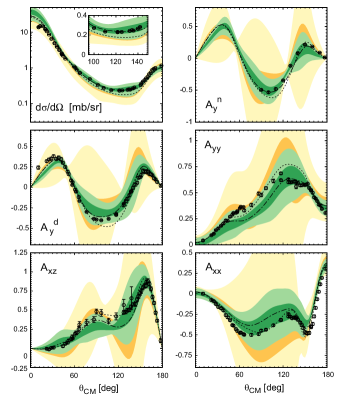
Figure 6.4: Predictions for the differential cross section, nucleon and deuteron analyzing powers $A^{n}_{y}$ and $A^{d}_{y}$ as well as deuteron tensor analyzing powers $A_{yy}$, $A_{xz}$, and $A_{xx}$ in elastic nucleon–deuteron scattering at a laboratory energy of 135 MeV at NLO (yellow bands) and NNLO (green bands). The light- (dark-) shaded bands indicate 95% (68%) confidence levels. The dotted (dashed) lines show the results based on the CD-Bonn $NN$ potential [12] (CD-Bonn $NN$ potential in combination with the Tucson-Melbourne 3NF [3]). Black symbols represent the data together with their experimental errors. (Reproduced from Ref. [223].)

One may conclude that not all calculations, which have been published in the literature under the label of ab initio, are really ab initio. Indeed, of the cases we considered here, only 50% pass the test. But we need to point out that even in the two cases we declared ab initio, there are concerns. The NNLO predictions by Hoppe and Hüther for finite nuclei barely overlap within their theoretical uncertainties and, for nuclear matter, they do not overlap at all. Obviously, there are problems with the error estimates and the uncertainties are much larger than the shown ones. The true NNLO truncation errors of the Hoppe and Hüther calculations are probably as large as the differences between the two predictions. In this way, the two predictions are actually consistent with each other, in spite of their seeming discrepancy. Chiral EFT is a model-independent theory and, thus, different calculations at the same order should agree within truncation errors.

At N³LO the predictions differ even more. However, for current N³LO calculations, a strong caveat is in place. As pointed out in Ref. [224], there is a problem with the regularized 3NF at N³LO (and higher orders) in all present nuclear structure calculations. The N³LO 3NFs currently in use are all regularized by a multiplicative regulator applied to the 3NF expressions that are derived from dimensional regularization. This approach leads to a violation of chiral symmetry at N³LO and destroys the consistency between two- and three-nucleon forces [224, 107]. Consequently, all current calculations that include a N³LO 3NF contain an uncontrolled error and are, therefore, unreliable. When a consistent regularization scheme has been found, the calculations have to be repeated. At the present time, reliable predictions exist only at NNLO, NLO, and LO.

6.1.3   The future: ab initio plus precision

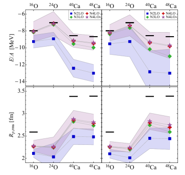
Figure 6.5: Latest ab initio predictions by the LENPIC collaboration [176]: Ground-state energies and point-proton radii for doubly magic oxygen and calcium isotopes obtained from the $NN$ potential of Ref. [91] complemented by NNLO 3NFs using a cutoff of 450 MeV (left-hand panel) and of 500 MeV (right-hand panel). The blue squares represent the predictions by complete NNLO calculations with the blue error bands showing the chiral NNLO truncation uncertainties at the 95% confidence level. The green and purple points and pink error bands are based upon incomplete calculations and are to be ignored. Black bars indicate the experimental data. (Reproduced from Ref. [176] with permission.)

It is encouraging to know that at least a few correct ab initio calculations do exist. But these cases show that the precision at NNLO is very poor. The same is true for the latest LENPIC calculations [176], see Fig. 6.5 (which we did not include in our case study, because nuclear matter results are lacking). At N³LO (if one day correct such calculations become available) the precision will most likely not be substantially better.

The purpose of the ab initio approach is to test if the tenet of nuclear theory is correct or not. Within huge errors as, e. g. in Fig. 6.4, any approach may come out right. So, that is not a good basis for a reliable test. We need more precision! This is in particular true for the 3NF and the reproduction of the 3$N$ data, which has been thoroughly investigated in Refs [223, 225] with the conclusion that, at N⁴LO, there is a chance to achieve the desirable precision—for several reasons. The long- and intermediate-range topologies of the 3NF at N⁴LO are expected to be much larger than the corresponding ones at N³LO because, at N⁴LO, the subleading $\pi NN$ seagull vertex is involved with LECs $c_{i}$, which are large [30, 43]. This will provide the 3NF at N⁴LO with more leverage as compared to N³LO. Moreover, at N⁴LO, 13 new 3$N$ contact terms occur [44] with essentially free parameters introducing considerable flexibility [45, 225] (see also Ref. [226]). Worth mentioning is also that, at N⁴LO, the 3NF includes all 20 operators of the most general 3NF [227]. Furthermore, the plentiful N⁴LO 3NF terms may also provide what is needed to improve the status of the medium-mass nuclei and nuclear matter.

Thus, the future of truly microscopic nuclear structure is to go for complete N⁴LO calculations—a gigantic task.

6.2   Infinite matter: A path to reach out to multiple systems, from nuclei to neutron stars

As discussed in the previous sections, during the past two decades there has been remarkable progress in understanding nuclear forces at a fundamental level, through the concept of EFT [18, 24]. Meson theoretic or entirely phenomenological models of the $NN$ interaction, augmented with phenomenological few-nucleon forces, are the typical paradigm used in the past. Within the framework of chiral EFT, we discussed applications to medium-mass nuclei.

We now move to infinite matter. Although an idealized system, its equation of state (EoS) is a powerful tool for exploring nuclear interactions in the medium. Isospin-asymmetric nuclear matter (IANM) is characterized by the degree of neutron excess, all the way to pure NM. Because neutrons do not form a bound state, the presence of excess neutrons in a nucleus reduces the binding energy, namely, it is a necessary but destabilizing effect which gives rise to the symmetry energy. As a consequence, neutron-rich structures have common features, which explain the formation of a neutron skin (in isospin-asymmetric nuclei) or the outward pressure in dense systems with high neutron concentration, which supports neutron stars against gravitational collapse. Studies of nuclear interactions in systems with high or extreme neutron to proton ratio are crucial towards understanding of the neutron driplines, the location of which is not well known. The new Facility for Rare Isotope Beams (FRIB), operational since May 2022, is expected to increase the number of known rare isotopes from 3000 to about 6000 [228].

After a brief discussion of SNM in Sec. 6.2.1, we focus on the NM EoS (Sec. 6.2.2) and the symmetry energy (Sec. 6.2.3). A focal point of this section is a comparison of ab initio predictions with phenomenological and empirical findings. Since many years, several groups have sought constraints on the density dependence of the symmetry energy. Intense experimental effort has been and continues to be devoted to this question using various measurements, which are typically analyzed with the help of correlations obtained through different parametrizations of phenomenological models. Popular examples are the Skyrme forces (Refs. [229, 230, 231] are only a few of the many review articles on the Skyrme model), and relativistic mean-field models (RMF) [232, 233, 234]. Reference [235] and Ref. [236] are representative applications of Skyrme forces or RMF models, respectively, to the issues confronted here. Generally, the extracted constraints vary considerably depending on the methods employed.

We follow with a discussion on the neutron skin, see Sec. 6.2.4, and its sensitivity to the density slope of the symmetry energy at saturation. We underline the sensitivity of the discussed predictions to free-space $NN$ scattering phases. In Sec. 6.2.4, we also present an extended analysis of current issues related to recent extractions of the neutron skins in ²⁰⁸Pb and ⁴⁸Ca from weak electron scattering measurements.

The density dependence of the symmetry energy is also a major component in the physics of neutron stars, in particular the radius of a medium-mass neutron star. Of course, a very large range of densities can be found in a neutron star, from the density of iron in the outer crust up to several times normal nuclear density in the core, and thus no theory of hadrons can be applicable over the entire range. With that in mind, state-of-the-art ab initio theories of SNM and NM can be taken as the foundation for any extension method, which will unavoidably involve some degree of phenomenology. Note, though, that the radius of a 1.4 M_⊙ neutron star is sensitive to the pressure in neutron matter around saturation, and thus it is useful to constrain microscopic theories of the EoS at those densities where the theories are reliable [237]. In fact, the radius of light to medium neutron stars has been found to correlate with the density slope of the symmetry energy at saturation, with correlation coefficient of 0.87 for $M=1.0M_{\odot}$ and 0.75 for $M=1.4M_{\odot}$ [238].

To advance our understanding of intriguing systems such as neutron skins and neutron stars, it is important to build on the enormous progress in nuclear theory since the days of one-boson-exchange or phenomenological $NN$ potentials and phenomenological 3NFs, selected with no clear scheme or guidance. Predictions from state-of-the-art nuclear theory favor a softer density dependence of the symmetry energy – on the low-to-medium end of the spectrum cited in the literature – and, naturally, smaller neutron skins and radii of canonical mass neutron stars.

The purpose and overarching theme of this section are to perform an analysis of existing literature addressing the nuclear symmetry energy, with the objective to identify and discuss current gaps or problems, and provide recommendations for future research. The diagram in Fig. 6.6 is a "flow chart" showing how the various applications we discuss are linked to one another and originate from a common source, state-of-the-art nuclear forces.

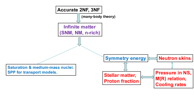
Figure 6.6: Schematic diagram showing the connections among the topics addressed in the remaining parts of this article. “SPP "stands for single-particle potential.

6.2.1   Symmetric nuclear matter

Constructing the equation of state (EoS) of infinite nuclear matter microscopically from state-of-the-art few-body interactions remains a very challenging problem in nuclear theory. The EoS gives fundamental insight into nuclear forces in the medium, and is a crucial input in a variety of fields, ranging from heavy-ion (HI) reactions to astrophysical processes.

In Sec. 6.1, we discussed the current problems with reconciling SNM saturation and bulk properties of medium-mass nuclei, as well as recently proposed unsuccessful solutions. In this section, we wish to discuss several aspects related to the EoS of SNM, from bulk to single-particle properties [171]. First, we will show order-by-order predictions for the EoS with errors quantified as described in Sec. 5.

After addressing bulk properties, we will study the impact of 3NFs on the single-particle potential. Single-particle energies, often parametrized in terms of effective masses, provide insight into both density and momentum dependence of the in-medium interaction, and are an important part of the input for transport calculations.

Theoretical tools.

In what follows, our highest-order predictions are obtained using $NN$ forces and 3NF consistently at N³LO. The chiral $NN$ potential is the one from Ref. [94], with cutoff equal to 450 MeV. To calculate the energy per nucleon in nuclear (or neutron) matter, we use the nonperturbative particle-particle ladder approximation, which generates the leading-order terms in the hole-line expansion of the energy per particle. We compute the single-particle spectrum self-consistently. The Bethe-Goldstone (or Brueckner) equation for two particles having center-of-mass momentum $\vec{P}$, initial relative momentum $\vec{q_{0}}$, and starting energy $\epsilon_{0}$ in nuclear matter with Fermi momentum $k_{F}$ is

$$G_{P,e_{0},k_{F}}(q,q_{0})=V(q,q_{0},k_{F})+\int_{0}^{\infty}dkk^{2}\frac{V(q,k,k_{F})Q(k,P,k_{F})G(k,q_{0},k_{F})}{\epsilon_{0}-(\epsilon(\vec{P}+\vec{k})+\epsilon(\vec{P}-\vec{k}))+i\delta}\;,$$ (6.1)

where the Pauli operator, $Q$, has been angle-averaged, and $V$ is the $NN$ potential augmented with effective 3NFs as density dependent potentials. When calculating the single-particle potential, $U$, one must recall that, in order to avoid double-counting, a factor of $1/2$ must be applied to the density-dependent part of $V$ at the Hartree-Fock level [239]:

$$V=V_{NN}+(1/2)V_{DD}\;,$$ (6.2)

where, again, the first term on the right-hand side is the actual $NN$ potential and the second one is a density-dependent effective 3NF. For the latter, we employ the density dependent $NN$ interactions derived in Refs. [240, 241, 242, 243] from the leading and subleading chiral three-body force. This effective interaction is obtained by summing one particle line over the occupied states in the Fermi sea, such that the resulting $NN$ interactions can be expressed in analytical or semi-analytical form with operator structures identical to those of free-space $NN$ interactions. A comprehensive review on implementation and applications of 3NFs [115] examines various approximations. We agree with the author of Ref. [115] that the analytical or semi-analytical approaches, while having the advantage of not requiring large input files of 3NF matrix elements, can quickly become cumbersome. As for the quantitative impact from this approximation, in Ref. [170] we examined different subleading contributions to the 3NF potential in neutron matter [244, 245] and found excellent agreement with the 3NF potentials from Ref. [168], where 3NFs are implemented differently, which we find encouraging.

Using partial wave decomposition, Eq.(6.1) can be solved for each partial wave using standard matrix inversion techniques. Note that the single-particle energy, $\epsilon$, contains the single-particle potential, $U$, yet to be determined. Because the G-matrix depends on $U$ and $U$ depends on $G$, an iteration scheme is applied to obtain a self-consistent solution for $U$ and $G$, which are related as:

$$U(k_{1},k_{F})=\int\ \langle\vec{q_{o}}|G_{P,e_{0},k_{F}}|\vec{q_{o}}\rangle d^{3}k_{2}(\vec{q_{o}},\vec{P})\;,$$ (6.3)

where $k_{1,2}$ are sincle-particle momenta. Starting from some initial values and a suitable parametrization of the single-particle potential, a first solution is obtained for the G-matrix, which is then used in Eq.(6.3). The procedure continues until convergence to the desired accuracy.

The energy per nucleon is then evaluated as:

$$\frac{E}{N}=\langle T(k_{1})\rangle_{(k_{F})}+\langle U(k_{1},k_{F})\rangle_{(k_{F})}\;,$$ (6.4)

where the averages of the single-nucleon kinetic ($T(k_{1})$) and potential ($U(k_{1},k_{F})$) energies are taken over the Fermi sea.

Some comments are in place regarding the choice of the many-body method we employ, namely the nonperturbative particle-particle ladder approximation. In the traditional hole-line expansion, the particle-particle ladder diagrams comprise the leading-order contributions. The next set of diagrams contains the three hole-line contributions, which includes the third-order particle-hole (ph) diagram considered in Ref. [111]. The third-order hole-hole (hh) diagram (fourth order in the hole-line expansion) was found to give a negligible contribution to the energy per particle at normal density regardless the cutoff (see Tables II and III of Ref. [111]). The ph diagram is relatively much larger, bringing in an uncertainty of about $\pm$ 1 MeV on the potential energy per particle at normal density.

Order by order predictions of the EoS.

We begin with the study displayed in Fig. 6.7. The curves are obtained with $\Lambda$ = 450 MeV and the different sets of $c_{D},c_{E}$ LECs displayed in Table 6.2, of which set (c) produces the best saturating behavior. The method used to fit the $c_{D},c_{E}$ LECs is described in the Supplemental Material of Ref. [155]. The first step is to impose that the chosen $NN$ and 3NF combination reproduces the ³H binding energy. The result is a trajectory in the $c_{D},c_{E}$ plane. The best pairs of couplings are then selected looking at the SNM saturation point, see Fig. 6.7.

On the left side of Fig. 6.8, we show the energy per nucleon from leading to fourth order. While the EoS has already a realistic behavior at the first order where 3NFs appear (N²LO), there is a definite improvement when moving to N³LO, for both saturation density and energy. This is an important validation of the predictive power of the chiral EFT – of course, $NN$ data and the three-nucleon system must be described accurately for any subsequent many-body predictions to be meaningful. On the right side, we displays the predictions at N³LO with the uncertainty band calculated from Eq. 5.5. We note that our N³LO(450) results for the energy per particle at saturation agree with those from Ref. [155] within uncertainties.

Table 6.2: Values of the LECs $c_{1,3,4}$, $c_{D}$, $c_{E}$, and $C_{S}$ and $C_{T}$ for different orders in the chiral EFT expansion. The momentum-space cutoff $\Lambda$ is equal to 450 MeV. The LECs $c_{1,3,4}$ are given in units of GeV^-1, $C_{S}$ and $C_{T}$ in units of $10^{4}$ GeV^-2, and $c_{D}$ and $c_{E}$ dimensionless. $c_{D}$, $c_{E}$ are taken from Ref. [155].

	$\Lambda$ (MeV)	$c_{1}$	$c_{3}$	$c_{4}$	$c_{D}$	$c_{E}$	$C_{S}$	$C_{T}$
N2LO	450	–0.74	–3.61	2.44	(a) 2.25	0.07	—	—
					(b) 2.50	0.1
					(c) 2.75	0.13
N3LO	450	–1.07	–5.32	3.56	(a) 0.00	-1.32	-0.011828	-0.000010
					(b) 0.25	-1.28
					(c) 0.50	-1.25

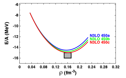
Figure 6.7: Energy per particle as a function of density at N³LO and cutoff equal to 450 MeV. The labels a, b, and c refer to the different sets of $c_{D},c_{E}$ values given in Table 6.2.

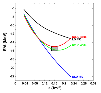
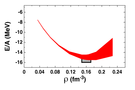
Figure 6.8: Left: Energy per particle as a function of density from leading to fourth order of the chiral expansion. Right: Energy per particle as a function of density at fourth order of the chiral expansion. The band shows the uncertainty calculated from Eq. 5.5. The cutoff is fixed at 450 MeV.

Single-particle properties.

While bulk properties of nuclear matter are very insightful for testing theories as well as providing a connection with bulk properties of nuclei, momentum- and density-dependent single-particle potentials (SPP) in nuclear matter provide complementary and more detailed information which is needed for heavy ion (HI) transport simulations.

Together with the SPP in neutron matter (NM), one can construct the momentum and density dependent SPP in IANM – and thus the so-called symmetry potential – to be used, for instance, in Boltzmann-Uehling-Uhlenbeck calculations of collective nuclear dynamics. A number of HI collision observables have been found to be sensitive to the symmetry potential, such as the neutron/proton ratio of pre-equilibrium nucleon emission, neutron-proton differential flow, and the proton elliptic flow at high transverse momenta.

Next, we will take a look at the underlying SPP, derived self-consistently from the Brueckner $G$-matrix and, thus, the EoS, to observe its momentum dependence and its changes with density and chiral order. First, for two selected densities (saturation density and about 2/3 of it, corresponding approximately to $k_{F}$ = 1.0 fm^-3), we show the single-particle potential at third and fourth order, Fig. 6.9.

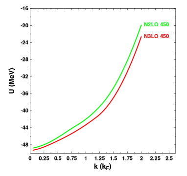
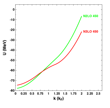
Figure 6.9: Predictions for the SPP at N²LO and N³LO in SNM. The cutoff is fixed at 450 MeV. For the left (right) frame, the Fermi momentum is equal to $k_{F}$ = 1.0 (1.333) fm^-1.

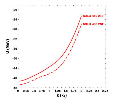
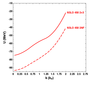
Figure 6.10: Impact of the 3NF at N³LO (solid curves) on the SPP at two different densities. Left: $k_{F}$ = 1.0 fm^-1; right: $k_{F}$ = 1.333 fm^-1. The cutoff is fixed at 450 MeV.

Single-particle potentials derived from chiral interactions are generally deep and grow monotonically from the bottom of the Fermi sea. The impact of moving to fourth order is much larger at the higher density.

The impact of including the complete 3NF up to N³LO is demonstrated in Fig. 6.10. The effect is to decrease the depth of the potential, and is strongly density dependent. This is a precursor of the repulsive and density dependent effect of the full 3NF on the average energy per nucleon.

Analyses of HI collision measurements are used to extract empirical constraints for the EoS. For instance, the elliptic flow in midperipheral to peripheral collisions was found to be particularly sensitive to the momentum dependence of the nucleon mean field [246]. More specifically, the connection between the quantities displayed in Fig. 6.9-6.10 and reaction data is through the nucleon isoscalar and isovector potentials, defined, respectively, as

$$U_{0}(k,\rho)=\frac{U_{n}+U_{p}}{2}\;$$ (6.5)

and

$$U_{sym}(k,\rho,\alpha)=\frac{U_{n}-U_{p}}{2\alpha}\;,$$ (6.6)

where $\alpha$ = $\frac{\rho_{n}-\rho_{p}}{\rho_{n}+\rho_{p}}$. Naturally, the isovector potential, also known as the symmetry potential, is relevant for reactions with neutron-rich nuclei. Of particular interest are rare isotopes, which can now be studied with radioactive isotope beams.

6.2.2   Neutron matter

The physics of NM spans a broad range of densities. At low density, it approaches universal behavior as a consequence of the large neutron-neutron scattering length in the spin-singlet channel. Around normal nuclear density, it is a convenient laboratory to study neutron-rich nuclei, and, at even higher densities, it strongly constrains the physics of neutron stars and, thus, the EoS of neutron-rich matter is the forefront of nuclear astrophysics. Although an idealized system, neutron matter also provides unique opportunities to test nuclear forces, because all low-energy couplings appearing in the three-neutron forces are predicted at the two-body level.

Theoretical predictions of neutron-rich matter are important and particularly timely, as they complement on-going and planned experimental efforts. Following PREX-II [247] and CREX [248], other experiments, such as MREX at MESA [249], seek to place constraints on the neutron radii and neutron skins of ⁴⁸Ca and ²⁰⁸Pb, and to further elucidate the relation between the neutron skin and the energy and pressure in neutron-rich matter.

Neutron stars are important natural laboratories for constraining theories of the EoS in neutron-rich matter, to which the mass-radius relationship of these stellar objects is sensitive. The radius of the average-mass neutron star is especially sensitive to the pressure gradient in neutron matter around normal densities [250]. Interest in these compact stars has increased considerably as we have entered the “multi-messenger era" of astrophysical observation. The GW170817 neutron star merger event has yielded new and independent constraints on the radius of a neutron star [251, 252]. More precisely, with the constraint that a mass of at least 2 M_⊙ [253] is supported by the EoS, the radii of the two neutron stars are reported as $R_{1}$ = (11.9 $\pm$ 1.4) km and $R_{2}$ = (11.9 $\pm$ 1.4) km, with the respective mass ranges constrained at (1.18 - 1.36) M_⊙ (for M₁) and (1.36 - 1.58) M_⊙ (for M₂) [254].

Energy per neutron in neutron matter.

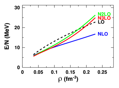
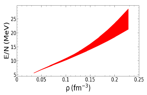
Figure 6.11: (Color online) Left: Energy per neutron in NM as a function of density, from leading order (black dash) to fourth order (solid red). Right: Energy per particle as a function of density at fourth order of the chiral expansion. The band shows the uncertainty calculated from Eq. 5.5. The cutoff is fixed at 450 MeV.

In Fig. 6.11, we show our results for the energy per neutron in neutron matter (NM) as a function of density over four orders, from LO to N³LO. We see large variations from leading order to the next, as to be expected at the lowest orders. It is interesting to notice the very large differences between NLO and N²LO, mostly due to the first appearance of 3NFs. The predictions at N³LO are slightly more attractive than those at N²LO, in agreement with other calculations [153].

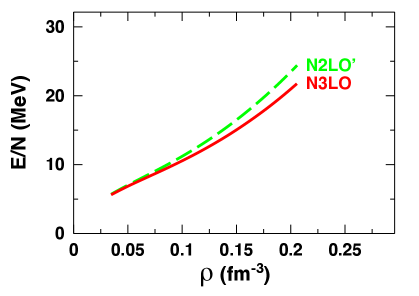
Figure 6.12: (Color online) Energy per neutron in NM as a function of density. The solid (red) curve is the same as in Fig. 6.11, while in the dashed green line (denoted by N²LO’), the N³LO 3NF contribution has been left out.

Figure 6.12 shows the impact of the subleading 3NF contribution only, comparing the result of the complete calculation at N³LO with the one obtained with the 2NF at N³LO and the leading 3NF only, model (N²LO^′). The effect is mildly attractive, about 2 MeV at the highest density, mostly due to the subleading 2PE 3NF.

The first four-nucleon forces (4NFs) appear at N³LO, but were found to be negligible [168, 161, 162]. Therefore, we omit them.

Our highest-order results for the energy per neutron at different densities are shown in the second column of Table 6.3 with their chiral uncertainty calculated as in Eq. (5.5). Our NM EoS is rather soft within the large spectrum of theoretical predictions in the literature, which is generally true for predictions based on chiral EFT. The degree of softness is best discussed in the context of density dependence of the symmetry energy, as we do next.

6.2.3   The symmetry energy

We begin with a pedagogical introduction to establish the main concepts and definitions.

The simplest picture of the nucleus goes back to the semi-empirical mass formula (SEMF), also known as the liquid-droplet model. Its ability to capture basic bulk features of nuclei is remarkable in view of its simplicity. The binding energy per nucleon is written in terms of a handful of terms inspired by the dependence of nuclear radii on the cubic root of the mass number A:

$$\frac{B(Z,A)}{A}=a_{V}-a_{sym}\frac{(A-2Z)^{2}}{A^{2}}-\frac{a_{s}}{A^{1/3}}-\frac{a_{C}Z(Z-1)}{A^{4/3}}-\frac{\Delta}{A}\;,$$ (6.7)

where the last term stands for additional, typically smaller, contributions. Note that the second term on the RHS depends on the relative neutron-proton asymmetry, or isospin asymmetry, $\frac{N-Z}{A}$, and represents the loss in binding energy experienced by a nucleus due to the destabilizing presence of asymmetry in neutron/proton concentrations. Of course, Eq. (6.7) is the simplest picture of a nucleus, but can be improved by replacing the number of nucleons $A$ and the number of protons $Z$ with the respective density profiles.

To that end, we introduce the energy per nucleon, $e(\rho,\alpha)$, in an infinite system of nucleons at density $\rho$ and isospin asymmetry $\alpha=\frac{\rho_{n}-\rho_{p}}{\rho}$ – namely, the EoS of neutron-rich matter – and expand this quantity with respect to the isospin asymmetry parameter:

$$e(\rho,\alpha)=e(\rho,\alpha=0)+\frac{1}{2}\Big{(}\frac{\partial^{2}e(\rho,\alpha)}{\partial\alpha^{2}}\Big{)}_{(\alpha=0)}\alpha^{2}+\mathcal{O}(\alpha^{4})\;.$$ (6.8)

Neglecting terms of order $\mathcal{O}(\alpha^{4})$, Eq. (6.8) takes the well-known parabolic form:

$$e(\rho,\alpha)\approx e_{0}(\rho)+e_{sym}(\rho)\ \alpha^{2}\;,$$ (6.9)

where $e_{sym}$ = $\frac{1}{2}\Big{(}\frac{\partial^{2}e(\rho,\alpha)}{\partial\alpha^{2}}\Big{)}_{\alpha=0}$ and $e_{0}(\rho)=e(\rho,\alpha=0)$, the EoS of SNM.

With the SEMF as a guideline, one can write the main contributions to the total energy of a given nucleus (Z,A) with proton and neutron density profiles $\rho_{p}(r)$ and $\rho_{n}(r)$, respectively, as:

$$\begin{split}E(Z,A)=\int d^{3}r\ \rho(r)\ e(\rho,\alpha)+f_{0}\int d^{3}r|\nabla\rho|^{2}+\frac{e^{2}}{4\pi\epsilon_{o}}(4\pi)^{2}\int^{\infty}_{0}dr^{\prime}\big{[}r^{\prime}\rho_{p}(r^{\prime})\int^{r^{\prime}}_{0}dr\ r^{2}\rho_{p}(r)\big{]}\end{split}\;,$$ (6.10)

where $f_{0}$ is a constant typically fitted to $\beta$-stable nuclei. Note that the second term on the RHS , dependent on the gradient of the density function, is a finite-size contribution – the surface term proportional to the coefficient $a_{s}$ in Eq. (6.7). The last term on the RHS stands for the Coulomb interaction among protons. The link to Eq. (6.7) is apparent. In particular, the first integral on the RHS of Eq. (6.10) comprises the first two terms on the RHS of Eq. (6.7).

Within the parabolic approximation (Eq. (6.9)), the symmetry energy becomes the difference between the energy per neutron in NM and the energy per nucleon in SNM:

$$e_{sym}(\rho)=e_{n}(\rho)-e_{0}(\rho)\;,$$ (6.11)

where $e_{n}(\rho)=e(\rho,\alpha=1)$, the energy per neutron in pure neutron matter.

The minimum of $e_{0}(\rho)$ at a density approximately equal to the average central density of nuclei, $\rho_{0}$, is a reflection of the saturating nature of the nuclear force. Next, we expand the symmetry energy about the saturation point:

$$e_{sym}(\rho)\ \approx\ e_{sym}(\rho_{0})+L\ \frac{\rho-\rho_{0}}{3\rho_{0}}+\frac{K_{sym}}{2}\frac{(\rho-\rho_{0})^{2}}{(3\rho_{0})^{2}}\;,$$ (6.12)

which helps identifying several useful parameters. $L$ is known as the slope parameter, as it is a measure of the slope of the symmetry energy at saturation:

$$L=3\rho_{0}\Big{(}\frac{\partial e_{sym}(\rho)}{\partial\rho}\Big{)}_{\rho_{0}}\;.$$ (6.13)

Furthermore, it is clear from Eqs. (6.11) and (6.13), recalling that the SNM EoS has vanishing derivative at that point, that $L$ measures the degree of “stiffness of the NM EoS at saturation density.

The parameter $K_{sym}$ characterizes the curvature of the symmetry energy at saturation density:

$$K_{sym}=9\ \rho_{0}^{2}\Big{(}\frac{\partial^{2}e_{sym}(\rho)}{\partial\rho^{2}}\Big{)}_{\rho_{0}}\;.$$ (6.14)

Using the standard thermodynamic relation,

$$P(\rho)=\rho^{2}\frac{\partial e}{\partial\rho}\;,$$ (6.15)

where $P$ is the pressure and $e$ is the energy per particle, we define the symmetry pressure as:

$$P_{sym}(\rho)=\rho^{2}\frac{\partial(e_{n}-e_{0})}{\partial\rho}=P_{NM}(\rho)-P_{SNM}(\rho)\;.$$ (6.16)

If the derivative is evaluated at or very near $\rho_{0}$, the symmetry pressure is essentially the pressure in NM because the pressure in SNM vanishes at saturation. Then:

$$P_{NM}(\rho_{0})=\Big{(}\rho^{2}\frac{\partial e_{n}(\rho)}{\partial\rho}\Big{)}_{\rho_{0}}\;.$$ (6.17)

From Eq. (6.13) and Eq. (6.17) it is clear that the slope parameter $L$ is a measure of the pressure in NM around saturation density:

$$P_{NM}(\rho_{0})=\rho_{0}\frac{L}{3}\;,$$ (6.18)

showing that the pressure in NM is proportional to the slope of the symmetry energy at normal density. The value of $L$ is then a measure of the pressure gradient acting on excess neutrons and pushing them outward from the neutron-enriched core of the nucleus to the outer region, thus determining the formation and size of the neutron skin.

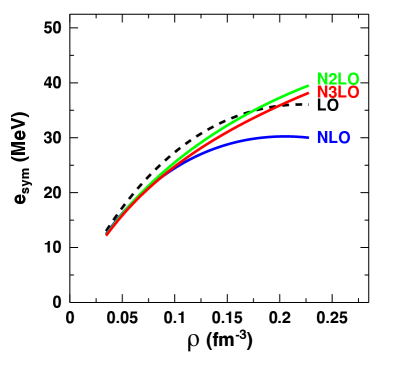
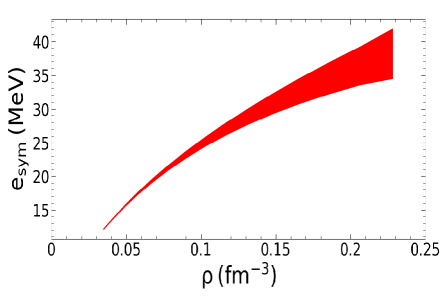
Figure 6.13: (Color online) Left: The symmmetry energy as a function of density, from leading order (black dash) to fourth order (solid red). Right: The symmetry energy as a function of density at fourth order of the chiral expansion. The band shows the uncertainty calculated from Eq. 5.5. The cutoff is fixed at 450 MeV.

Our order-by-order predictions for the symmetry energy are displayed in Fig. 6.13, and our results at N³LO together with their truncation errors are given in Table 6.3. To understand the full implications of these predictions, several comments are in place. To study correlations, phenomenological models are parameterized so as to ensure that the empirical saturation properties are well described, while the models can differ wildly in the isovector properties. Earlier investigations with a family of Skyrme interactions concluded that there is a linear correlation between the slope parameter and the neutron skin thickness of ²⁰⁸Pb [235]. This inherent connection between the symmetry energy density derivative and the neutron skin of neutron-rich nuclei is of great interest, because accurate measurements of the skin should then allow to set stringent constraints on the density dependence of the symmetry energy around saturation.

Relativistic mean-field models predict a very wide range of $L$ values, for example IU-FSU [255] gives 47.2 MeV for $L$, while NL3 [256] yields a value of 118.2 MeV. Naturally, these models also produce a large range of neutron skin values. For neutron skin predictions from RMF models, see also Ref. [257], where the authors utilize a large set of RMF models constrained by accurate fits of the nuclear binding energies and charge radii.

Constrains on $L$ vary considerably depending on the methods employed  [258, 259]. Analyses that employ laboratory data to extract constraints on the density dependence of the symmetry energy can be found in Refs. [260, 261, 262, 263, 264, 265, 266, 267, 268, 269]. Constraints on the symmetry energy and its density dependence have also been sought through techniques, such as: data on nuclear masses across the periodic table [270], giant dipole resonance energies [271], electric dipole polarizability [272], measurements of directed and elliptic flows in heavy ion (HI) collisions [269], isobaric analog states [264], isospin diffusion in HI collisions [273], neutron and proton transverse emission ratio measurements [274], HI collisions at intermediate energies [275]. As for the symmetry energy curvature, Eq. (6.14), constraints carry a much larger uncertainty [276, 277, 278].

In addition to the energy per neutron at saturation density, we show in Table 6.3 the symmetry energy at saturation, the slope parameter as defined in Eq. (6.13), and the pressure in neutron matter. As mentioned earlier, a softer nature is typical of chiral predictions, see, for instance, Ref. [279], where SRG-evolved interactions based on the potentials from Ref. [38] and the leading 3NF are employed. A comparison with phenomenological interactions of the past, such as Argonne V18 and the UIX 3NF [147], is given in Ref. [279]. For a more recent analysis, see Ref. [169], where the reported values for $e_{sym}(\rho_{o})$ and $L$ are (31.7 $\pm$ 1.1) MeV and (59.8 $\pm$ 4.1) MeV, respectively.

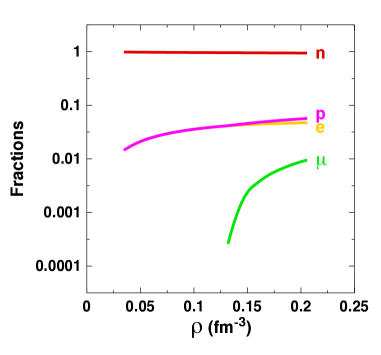
Figure 6.16: (Color online) Particle fractions as a function of density in $\beta$-equilibrated matter with neutrons, protons, electrons, and muons.

On the other hand, values such as those shown in the first row of Table 6.3 – approximately $L$=(50 $\pm$ 10) MeV, and pressure at $\rho_{o}$ between 2 and 3 MeV/fm³– are nowhere near those extracted from the PREX-II experiment [247], which are: $e_{sym}$ = (38.29 $\pm$ 4.66) MeV and $L$ = (109.56 $\pm$ 36.41) MeV. The corresponding value of the pressure at $\rho_{o}$ is then, approximately, between 3.66 MeV/fm³ and 7.30 MeV/fm³. Furthermore, such stiff symmetry energy would allow rapid cooling through direct Urca processes to proceed at unusually low values of the neutron star mass and central density [247], which seems unlikely [280]. The various particle fractions in $\beta$-stable matter that we obtain with our N³LO predictions are shown in Fig. 6.16. The proton fraction is close to 6% at $\rho\approx$ 0.2 fm^-3, still far from the direct Urca threshold of approximately 11%.

Back to Table 6.3, we also show the predictions at some specific densities below $\rho_{o}$. These are the densities identified in Ref. [281] as “sensitive" densities from the slope of the correlation in the plane of $e_{sym}(\rho_{o})$ vs. $L$ obtained from the measurements of a specific observable. In fact, a particular slope reflects a specific density at which that observable is especially sensitive to the symmetry energy. Our ab initio predictions and the values taken from Ref. [281] shown in Table 6.3, compare favorably within uncertainties. We recall that, at $\rho$ = (2/3)$\rho_{o}\approx$ 0.1 fm^-3 (an average between central and surface densities in nuclei), the symmetry energy is well constrained by the binding energy of heavy, neutron-rich nuclei [247] – hence, the relevance of this density region for the purpose of correlations between $L$ and the neutron skin of ²⁰⁸Pb.

Finally, in Table 6.4 we show our predictions for $K_{sym}$, defined in Eq. (6.14), in comparison with recent constraints [281]. Given the strong sensitivity of $K_{sym}$ to the details of the symmetry energy curvature, this parameter is very model dependent and difficult to constrain, with reported values ranging from large and negative to large and positive. As seen from Table 6.4, our predictions are in reasonable agreement with the constraints discussed in Ref. [281].

It is our understanding that, focusing on the sensitive density for a given observable, better consistency among different analyses can be found [281]. Perhaps these considerations may help with the interpretation of the large values from PREX-II. When the current constraint from PREX-II is included in the fits, its impact is weak due to the large experimental uncertainty [281]. For the slope of the symmetry energy at $\rho$ = (2/3)$\rho_{o}\approx$ 0.1fm^-3, the value obtained from PREX-II data [247] is $L$ =(73.69 $\pm$ 22.28) MeV.

Table 6.3: The energy per neutron, the symmetry energy, the slope parameter, and the pressure at N³LO at various densities, $\rho$, in units of $\rho_{o}$=0.155 fm^-3. $L$ is defined as in Eq. (6.13) at the specified density. The values in parentheses are taken from Ref. [281]. The constraint for $L$ in the third row ($\rho=0.67\rho_{o}$) is given for $\rho$=0.1 fm^-3. The constraint at $\rho=0.31\rho_{o}$ is from Ref. [282].

$\rho$ $(\rho_{o})$	$\frac{E}{N}(\rho)$ (MeV)	$e_{sym}(\rho)$ (MeV)	$L(\rho)$(MeV)	$P_{NM}(\rho)$ (MeV/fm3)
1	15.67 $\pm$ 1.13	31.67 $\pm$ 1.64 (33.3 $\pm$ 1.3)	49.84 $\pm$ 8.71 (59.6 $\pm$ 22.1)	2.52 $\pm$ 0.45 (3.2 $\pm$ 1.2)
0.72 (0.72 $\pm$ 0.01)	11.55 $\pm$ 0.41	26.45 $\pm$ 0.82 (25.4 $\pm$ 1.1)	45.59 $\pm$ 3.49	1.05 $\pm$ 0.13
0.67 (0.66 $\pm$ 0.04)	10.87 $\pm$ 0.35	25.30 $\pm$ 0.69 (25.5 $\pm$ 1.1)	44.41 $\pm$ 2.67 (53.1 $\pm$ 6.1)	0.86 $\pm$ 0.09
0.63 (0.63 $\pm$ 0.03)	10.42 $\pm$ 0.32	24.47 $\pm$ 0.61 (24.7 $\pm$ 0.8)	43.79 $\pm$ 2.28	0.75 $\pm$ 0.07
0.31 (0.31 $\pm$ 0.03)	6.72 $\pm$ 0.08	15.43 $\pm$ 0.12 (15.9 $\pm$ 1.0)	32.44 $\pm$ 0.51	0.18 $\pm$ 0.01
0.21 (0.22 $\pm$ 0.07)	5.44 $\pm$ 0.04	11.63 $\pm$ 0.04 (10.1 $\pm$ 1.0)	26.09 $\pm$ 0.11	0.096 $\pm$ 0.001

Table 6.4: Predictions for the parameter $K_{sym}$ at N³LO and constraints for $K_{sym}$ from Ref. [281] at two densities.

$\rho(\rho_{o})$	$K_{sym}(\rho)$ (MeV)	$K_{sym}(\rho)$ (MeV) from Ref. [281]
1	-102 $\pm$ 30	-180 $\pm$ 96
$\frac{2}{3}$	-76.5 $\pm$ 11.5	-79.2 $\pm$ 37.6

6.2.4   Neutron skins

Here, we link the EoS described in Sec. 6.2.1 and 6.2.2 to the neutron skin, defined as

$$S=<r^{2}>_{n}^{1/2}-<r^{2}>_{p}^{1/2}\;.$$ (6.19)

Relating the nucleus spatial extension as directly as possible to the microscopic EoS is best achieved by means of the droplet model [283]. This also allows applications to heavy nuclei, which may be outside the reach of ab initio methods. The predictions in Table 6.5 are taken from Ref. [284]. Those are calculated from droplet model expressions where the symmetry energy and its density slope at saturation appear explicitely.

Table 6.5: The neutron skin of ²⁰⁸Pb, $S$, calculated as described in Ref. [284] using the specified symmetry energy, $J$, and its slope at saturation, $L$.

$J$ (MeV)	$L$ (MeV)	$S$ (fm)	source for $J$, $L$
31.3 $\pm$ 0.8	52.6 $\pm$ 4.0	[0.13, 0.17]	[285]
(31.1, 32.5)	[44.8, 56.2]	[0.12, 0.17]	[155]
(28, 35)	[20, 72]	[0.078, 0.20]	[286]
(27, 43)	[7.17, 135]	[0.055, 0.28]	[287]
38.29 $\pm$ 4.66	109.56 $\pm$ 36.41	[0.17, 0.31]	[247]

Table 6.6: Values of the neutron skins in ⁴⁸Ca and in ²⁰⁸Pb from a variety of experimental methods. It is our understanding that the quoted errors refer to one standard deviation. For the values taken from Ref. [288] and Ref. [289], the first and second uncertainties are statistical and systematic errors, respectively. In Ref. [290], the first uncertainty is the experimental error, while the second originates from theoretical modeling of the experimental charge densities. Finally, in the result from Ref. [291], the first two uncertainties are the experimental and the theoretical error, respectively, and the third one stands for an estimated uncertainty in the symmetry energy at saturation.

Type of measurement	Extracted neutron skin in 48Ca	Extracted neutron skin in 208Pb
Proton-nucleus scattering [292]	0.056 - 0.102	0.083 - 0.111
Proton-nucleus scattering [293]		0.211${}^{+0.054}_{-0.063}$
Proton-nucleus scattering [294]		0.20 $\pm$ 0.04
Proton-nucleus scattering [295]	0.10 $\pm$ 0.03
Polarized proton-nucleus scattering [296]	0.23 $\pm$ 0.05	0.16 $\pm$ 0.05
Polarized proton-nucleus scattering [297]	0.168${}^{+0.025}_{-0.028}$
Polarized proton-nucleus scattering [293]		0.211 ${}^{+0.054}_{-0.063}$
Pionic probes [298]	0.13 $\pm$ 0.06	0.11 $\pm$ 0.06
Pionic probes [299]	0.11 $\pm$ 0.04
Coherent $\pi$ photoproduction [288]		0.15 $\pm$ 0.03${}^{+0.01}_{-0.03}$
Coherent $\pi$ photoproduction [300]		0.20 ${}^{+0.01}_{-0.03}$
Antiprotonic atoms [290]		0.20 ($\pm$ 0.04) ($\pm$ 0.05)
Antiprotonic atoms [289]		0.16 ($\pm$ 0.02) ($\pm$ 0.04)
Antiprotonic atoms [301]		0.15 $\pm$ 0.02
Electric dipole polarizability [265]		0.13 - 0.19
Electric dipole polarizability [291]		0.165 ($\pm$0.09)($\pm$ 0.013) ($\pm$0.021)
Electric dipole polarizability
via polarized scattering at forward angle [266]		0.156 ${}^{+0.025}_{-0.021}$
Electric dipole polarizability [272]	0.14 - 0.20
Pygmy dipole resonances [302]		0.18 $\pm$ 0.035
Interaction cross sections [303]	0.105 $\pm$ 0.06
$(\alpha,\alpha^{\prime})$ GDR 120 MeV [304]		0.19 $\pm$0.09
$\alpha$-particle scattering [305]	0.171 $\pm$ 0.05

The first three entries in Table 6.5 are obtained from EoS based on chiral EFT, with chiral two- and three-nucleon interactions at N³LO. One can see that they are relatively soft, cover a narrow range, and are in good agreement with one another. Consistent with earlier discussions, the corresponding neutron skins are relatively small. Most recently, ab initio predictions for the neutron skin of ²⁰⁸Pb have become available [306]. The reported range is between 0.14 and 0.20 fm, smaller than the values extracted from parity violating electron scattering. The fourth line corresponds to an analysis based on current constraints from nuclear theory and experiment. In Ref. [287], the authors utilized 48 phenomenological models, both relativistic mean field and Skyrme Hartree-Fock. The last line shows the values of $J$ and $L$ from the PREX II experiment. Note that the reported value for the skin of ²⁰⁸Pb in Ref. [247] is (0.283 $\pm$ 0.071) fm, giving a range between 0.21 and 0.35 fm.

Experiments and phenomenological analyses.

Indirect measurements of the neutron skin in ²⁰⁸Pb and ⁴⁸Ca have been performed using a variety of techniques, such as those listed below. Parity-violating electron scattering will be addressed separately. Some representative measurements are: Proton-nucleus elastic scattering [292, 293, 294, 295]; Polarized proton-nucleus elastic scattering [296, 297]; Pionic probes [298, 299]; Coherent pion photoproduction [288]; Antiprotonic atom data [290, 289, 301]; Electric dipole polarizability [265, 291, 266, 272]; Pygmy dipole resonsnces [302]; Interaction cross sections with microscopic optical potentials [303]; $(\alpha,\alpha^{\prime})$ giant dipole resonance (GDR) [304]; $\alpha$-particle scattering [305];

In Table 6.6, we summarize values for ²⁰⁸Pb and ⁴⁸Ca neutron skins deduced from the indicated experiments. There is a considerable spread, as the result of a multitude of methods and theoretical input over decades. Analyses of hadronic scattering experiments, in particular, require modeling of the nuclear potential.

The parity-violating experiment to measure the neutron skin of ⁴⁸Ca was recently completed [248].The extracted value of the neutron skin, $S=0.121\pm 0.026\pm 0.024$, would not be expected based on PREX-II. In the words of one of the CREX collaboration member, K.D. Paschke, “…the contrast between the two measurements is a bit surprising and provides a challenge to the theoretical description of nuclei." The results from CREX and PREX-II are not consistent with each other because the two nuclei are rather similar with regard to isospin asymmetry, see Fig. 6.14. Our findings for ²⁰⁸Pb are consistent with the CREX reported value for ⁴⁸Ca (both on the smaller side): S(⁴⁸Ca) = 0.12 – 0.15 fm and S(²⁰⁸Pb) = 0.13 – 0.17 fm. Based on previous measurements of the skin in ⁴⁸Ca, we see no strong reasons to deem the CREX result surprising or unexpected, whereas the opposite is true for ²⁰⁸Pb. A more in-depth discussion follows below.

Parity-violating electron scattering.

The parity-violating electron scattering asymmetry, $A_{PV}$, is defined for a spin-zero nucleus as

$$A_{PV}=\frac{\sigma_{R}-\sigma_{L}}{\sigma_{R}+\sigma_{L}}\;,$$ (6.20)

where $\sigma_{R(L)}$ is the elastic cross section for right (left) handed electrons [307]. $A_{PV}$ is proportional to the ratio of weak ($F_{W}(q)$) to charge ($F_{ch}(q)$) form factors, whith $q$ the four-momentum transfer. $F_{ch}(q)$ is taken from existing measurements and $F_{W}(q)$ is extracted from the measured $A_{PV}$. We recall that the weak and charge form factors are the Fourier transforms of the weak charge density and the charge density, respectively:

$$F_{W}(q)=\frac{1}{Q_{W}}\int d^{3}rj_{0}(qr)\rho_{W}(r)\;,$$ (6.21)

where $Q_{W}$ is the weak charge of the nucleus, and

$$F_{ch}(q)=\frac{1}{Z}\int d^{3}rj_{0}(qr)\rho_{ch}(r)\;.$$ (6.22)

In Eqs. (6.21) and (6.22), $j_{0}(qr)$ is the zero^th order spherical Bessel function. In Eq. (6.21), a form is assumed for $\rho_{W}(r)$ and the radius parameter of the density function is adjusted to reproduce the experimental $A_{PV}$. A form must also be assumed for $\rho_{ch}$ in Eq. (6.22), but its parametrization relies upon well-established measurements from charged electron scattering. The CREX result is found insensitive to the assumed form for the weak charge density [248].

Status of neutron skin predictions from ab initio theory.

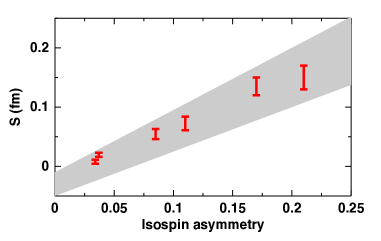
Figure 6.14: (Color online) Red bars: Neutron skin of ⁵⁸Ni, ²⁷Al, ⁵⁹Co, ⁹⁰Zr, ⁴⁸Ca, and ^208Pb, in order of increasing isospin asymmetry, as predicted in Refs. [284]. The shaded area is bounded by linear fits to the data [283].

Table 6.7: Status of ab initio predictions for the skins (in fm) in ⁴⁸Ca and in ²⁰⁸Pb. The two results from Ref. [308] for both ⁴⁸Ca and in ²⁰⁸Pb show acceptable ranges within 68% and 90% of the credibility region (CR). The last two entries were obtained from density functional theory [309].

Nucleus	Predicted skin	Source
48Ca	0.120 - 0.150	Ref. [310]
48Ca	0.141 - 0.187	Ref. [308] 68% CR
48Ca	0.123 - 0.199	Ref. [308] 90% CR
208Pb	0.139 - 0.200	Ref. [308] 68% CR
208Pb	0.120 - 0.221	Ref. [308] 90% CR
48Ca	0.114 - 0.186	Ref. [311]
208Pb	0.184 - 0.236	Ref. [311]
48Ca	0.12 - 0.15	Ref. [284]
208Pb	0.13 - 0.17	Ref. [284]
48Ca	0.176 $\pm$ 0.018	Ref. [309]
208Pb	0.168 $\pm$ 0.022	Ref. [309]

We show in Table  6.7 recent predictions for the skins in ⁴⁸Ca and in ²⁰⁸Pb. Some comments are in place. In both Ref. [310] and Ref. [311], the nature of the $NN$ chiral potentials, N²LO_sat (see Table 3.1 for characteristics of the various potentials), and $\Delta$N²LO_GO (see Table 3.1 ). is such that the results are not truly ab initio. Note, also, that the value for ²⁰⁸Pb from Ref. [311] is not a prediction, but was obtained using the linear regression the authors constructed from the skins of lighter nuclei.

Figure 6.15 shows the neutron skin in ⁴⁸Ca vs. the one in ²⁰⁸Pb. All values, except for the green bars, have been extracted from Fig. 5 of Ref. [248]. The PREX-II and PREX-I combined experimental result is shown by the blue bar, while the red vertical bar is the CREX result. The gray circles (pink diamonds) show results from a variety of relativistic (non-relativistic) density functionals, which give values of the $L$ parameter ranging from small and negative to large and positive. Coupled cluster (CC) [310, 311] and dispersive optical model (DOM) predictions [312] are also displayed. Our predictions are shown by the green bars [284]. There exist, of course, RMF models that agree with the PREX result, and, correspondingly, generate values for ⁴⁸Ca that are also on the larger side.

We conclude that a value between 0.212 fm and 0.354 fm (0.283 $\pm$ 0.071) for the skin of ²⁰⁸Pb is outside the boundaries set by microscopic theory. Simultaneous consistency with both CREX and PREX seems to be a challenge even for phenomenology.

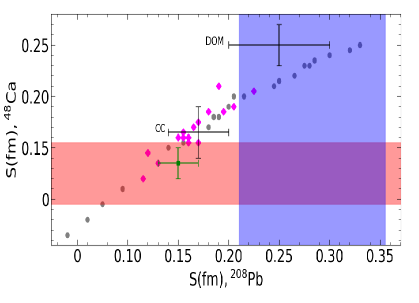
Figure 6.15: (Color online) The neutron skin of ⁴⁸Ca vs. the one of ²⁰⁸Pb. The red and blue bands show the results from CREX and combined PREX-I and PREX-II, respectively. The gray circles and pink diamonds are the result of relativistic and non-relativistic mean-field models, respectively. Coupled cluster and dispersive optical model predictions are indicated as CC and DOM, respectively.

We look forward to hearing from MREX (Mainz Radius Experiment) at the MESA accelerator. The MREX experiment promises to determine “…the neutron-skin thickness of ²⁰⁸Pb with ultimate precision." [249].

6.2.5   Equation of state for stellar matter

In this section we outline the main steps to construct the EoS for stellar matter in $\beta$-equilibrium. We define the total energy per baryon as:

$$e_{T}(\rho)=e_{0}(\rho)+e_{sym}\ (Y_{n}-Y_{p})^{2}+e_{e}+e_{\mu}+\sum_{i=n,p}Y_{i}m_{i}\;,$$ (6.23)

where $Y_{n,p}$ stands for the neutron or proton fraction. The last term accounts for the baryon rest energy, while $e_{e/\mu}$ are the energies (per baryon) of the electrons and muons, respectively. All terms are functions of density.

The energy density ($\epsilon_{i}$), pressure ($p_{i}$), number density ($\rho_{i}$) and chemical potential ($\mu_{i}$) for each lepton species, $i$, at a given Fermi momentum, $(k_{F})_{i}$, can be expressed as:

$$\epsilon_{i}=\frac{\gamma}{2\pi^{2}}\int^{k_{F_{i}}}_{0}\sqrt{k^{2}+m_{i}^{2}}\ k^{2}\ dk\;,$$ (6.24)

$$p_{i}=\frac{1}{3}\frac{\gamma}{2\pi^{2}}\int^{k_{F_{i}}}_{0}\frac{k^{2}}{\sqrt{k^{2}+m^{2}_{i}}}\ k^{2}\ dk\;,$$ (6.25)

$$\rho_{i}=\frac{\gamma}{2\pi^{2}}\int^{k_{F_{i}}}_{0}k^{2}\ dk\;,$$ (6.26)

$$\mu_{i}=\frac{\partial\epsilon_{i}}{\partial\rho_{i}}=\sqrt{k^{2}_{F_{i}}+m_{i}^{2}}\;,$$ (6.27)

where $\gamma$ is the spin/isospin degeneracy factor.

The energy per volume is obviously related to the energy per particle:

$$\epsilon=\rho\;e(\rho)\;,$$ (6.28)

Generally, the particle fraction,

$$Y_{i}=\frac{\rho_{i}}{\rho}\;,$$ (6.29)

is related to the chemical potential through:

$$\mu_{i}=\frac{\partial\epsilon_{i}}{\partial\rho_{i}}=\frac{\partial e_{i}}{\partial Y_{i}}\;.$$ (6.30)

From the condition of energy minimization, subjected to the constraints of conserved nucleon density and global charge neutrality,

$$\rho_{p}+\rho_{n}=\rho\quad\mbox{or}\quad Y_{p}+Y_{n}=1\;,$$ (6.31)

$$\rho_{p}=\rho_{e}+\rho_{\mu}\quad\mbox{or}\quad Y_{p}=Y_{e}+Y_{\mu}\;,$$ (6.32)

one can obtain all particle fractions. The proton fraction plays a major role in the cooling process of neutron stars, therefore, cooling data have the potential to shed light on the symmetry energy, closely related to the proton fraction in $\beta$-equilibrated matter. Below, we give a simple demonstration of this very direct relation.

Neglecting, for simplicity, the muon contribution ($Y_{p}$ = $Y_{e}$), the equations above give:

$$e_{e}=\frac{\hbar c}{4\pi^{2}}\rho^{1/3}(3\pi^{2}Y_{p})^{4/3}\,$$ (6.33)

$$\frac{\partial e_{e}}{\partial Y_{p}}=\frac{\hbar c}{3\pi^{2}}(3\pi^{2})^{4/3}(\rho Y_{p})^{1/3}\;,$$ (6.34)

$$\frac{\partial e_{p}}{\partial Y_{p}}=\frac{\partial e_{n}}{\partial Y_{n}}-\frac{\partial e_{e}}{\partial Y_{e}}\;,$$ (6.35)

from which we obtain:

$$4\ e_{sym}(\rho)\ (1-2\cdot Y_{p})=\hbar c(3\pi^{2})^{\frac{1}{3}}(\rho\ Y_{p})^{\frac{1}{3}}\;,$$ (6.36)

where we have neglected the mass difference between the proton and the neutron.

If $\rho_{DU}$ is the density at which $Y_{p}$ is equal to the value needed for direct Urca processes (DU), about $1/9$, the following relation holds:

$$e_{sym}(\rho_{DU})=\hbar c\frac{9}{28}(\pi^{2}/3)^{\frac{1}{3}}(\rho_{DU})^{1/3}\;.$$ (6.37)

This simple relation is quite insightful. If, for example, $\rho_{DU}$ is close to saturation density, the symmetry energy would be over 50 MeV at that point. If $\rho_{DU}=\frac{2}{3}\rho_{0}$, the symmetry energy at that density would be over 40 MeV. In our and other microscopic predictions, DU processes are more likely to open at a few to several times normal density (based on projections, since chiral EFT predictions cannot be extended to such high densities). Using PREX II constraints, the Urca threshold is found to be approximately 1.5$\rho_{0}$ or just above 0.2 $fm^{-3}$ [313]. From Eq. (6.37), the value of the symmetry energy at 1.5$\rho_{0}$ is then about 58 MeV, clearly indicationg an unusually steep density dependence, taking the PREX II value of 38.1 $\pm$ 4.7 MeV at saturation.

As noted above, the CREX experiment [248] is now completed and the results are not consistent with PREX II. The authors of Ref. [313] developed different parametrizations of RMF models constrained by CREX results, PREX II results, or a combination of both, and report that the direct Urca threshold density decreases from 0.71 fm^-3 to 0.21 fm^-3 as the skin of ²⁰⁸Pb increases from 0.13 fm to 0.28 fm.

At normal nuclear densities, typical predictions of the symmetry energy are consistent with a proton fraction approximately equal to 1/25 [314], far from the DU threshold. On the other hand, including PREX-II constraints, the threshold density for DU is found to be as low as 1.47$\rho_{0}$, with a threshold mass of 0.736 solar masses [315].

6.3   Astrophysics implications

A neutron star is the remnant collapsed core of a giant star which has undergone a supernova explosion. A star must have sufficient mass, estimated to be between 8 and 25 $M_{\odot}$, to undergo a supernova event at the end of its life cycle [316]. Due to its extremely compact nature, the neutron star is supported against further gravitational collapse into a black hole by mechanisms of nuclear origin, which make these objects excellent natural laboratories for exploring the nuclear EoS.

We begin this section by reviewing the relevance of neutron stars for nuclear physics, from a historical perspective. In 1934, just two years after the discovery of the neutron [317], Baade and Zwicky proposed the existence of a very dense stellar object, which they named neutron star, arising from the remnants of a supernova [318, 319]. In 1939 Tolmann [320], and, independently, Oppenheimer and Volkoff [321], estimated the mass–radius relationship of these neutron stars based on general relativity and crude models for the nuclear force, and developed the famous Tolmann–Oppenheimer–Volkoff (TOV) equation. The TOV equation allows to predict a theoretical upper limit on the possible mass of neutron stars. However, due to the very limited understanding of nuclear interactions at the time, their predictions were not accurate. With improved understanding of nucleonicEnergy emission from a neutron star interactions, a more realistic picture of neutron stars and their structure emerged [322, 323, 324, 325, 326, 327, 328, 329, 330, 331].

While the existence of neutron stars was theoretically possible, finding evidence of their existence remained a challenge. Initial attempts to compute and observe the thermal signature of neutron stars [332, 326, 333] were unsuccessful. In 1967, Pacini [334] postulated that fast rotating neutron stars could generate electromagnetic emission from a powerful magnetic dipole. Soon after, Bell and Hewish [335] discovered the first radio pulsar, characterized by a stable periodic electromagnetic signal. Later that year, Gold theorized that neutron stellar objects were suitable candidates to explain the unusual characteristics of the pulsar signal [336].

The connection between supernovas and pulsars was firmly established in 1969, with the discoveries of the Vela [337] and Crab Nebula [338] pulsars. Hundreds of pulsars were discovered in the 1970s and 1980s using radio astronomy, while more recent developments have identified pulsars whose signals span the electromagnetic spectrum [339]. To date, more than two and a half thousand pulsars have been discovered [340], in many configurations, such as binary pulsar systems [341], main-sequence binary-pulsar systems [342], globular clusters [343] with orbiting exo-planets [344], and displaying a wide variety of unusual periodic, signals [345, 346]. The relatively recent GW170817 neutron star merger event, detected through gravitational wave signatures by LIGO/Virgo [347] along with the accompanying gamma-ray burst [A_etal_2_2017], generated additional observational data.

While the neutron star radius cannot be measured directly, the mass of neutron stars in binary systems can be inferred from observation together with the application of gravitational theory. With constraints on the mass of a star, observational data allow for indirect inference of the radius, for instance through Doppler shift [339]. Observation-based constraints consistently place the estimated radius of a neutron star in the range of 10–15 km. Using accreting and bursting sources, the radius of the canonical-mass neutron star was determined to be within a range of 10.4 to 12.9 km [348], while analysis from the LIGO/Virgo observations determined the radius to be between 11.1 and 13.4 km [349]. Upper limits on the neutron star radii, as determined from iron emission lines, were placed between 14.5 and 16.5 km [350].

The mass range deduced from observed neutron stars is around 1–2 $M_{\odot}$. To date, the smallest mass neutron star has been determined to be $\approx$ 1.17 $M_{\odot}$ [351], while the most massive observed neutron star is $\approx$ 2.14 $M_{\odot}$ [352]. We recall that the Chandrasekhar mass limit of white dwarf stars is 1.4 $M_{\odot}$. If this mass is exceeded, electron degeneracy would no longer be able to support a white dwarf star from gravitational collapse. Observational constraints on neutron star masses yield values clustered around 1.4 $M_{\odot}$ [353] and for this reason this value is taken as the neutron star canonical mass. This also led to the idea that white dwarf collapse may be an additional mechanism for the formation of neutron stars [354, 355, 356].

Neutron star models are generally in good agreement with observational constraints for the radius. For instance, the radius of the canonical-mass neutron star predicted from the set of EoS applied in Ref. [357] is predicted to be in the range 10.45–12.66 km. From a variety of techniques, based on experimentally determined quantities correlated to symmetry energy parameters, the radius is determined to be between 10.7 and 13.1 km [358, 359, 357], while using a range of theoretical models a limit of 9.7 to 13.9 km is obtained [360, 361, 357]. Recent surveys of neutron star physics and theoretical approaches include Refs. [362, 363, 364].

On theoretical grounds, the largest mass was predicted to be 3.2 $M_{\odot}$ [365], based on only three assumptions: (1) General Relativity is the appropriate theory to describe these massive stars; (2) the EoS is constrained by Le Chatelier’s principle ($\partial P$/$\partial\epsilon\geq$ 0); (3) the causality condition, which constrains the speed of sound in dense matter to remain below the speed of light. While such massive neutron stars may be theoretically possible, none has been observed.

Over the past few years, interest in compact stars has increased considerably as we have entered the “multi-messenger era” of astrophysical observations. The GW170817 neutron star merger event has yielded new and independent constraints on the radius of the canonical mass neutron star [347]. Astronomy with gravitational waves provides additional opportunities to explore these exotic systems.

The remarkable point is that the EoS of neutron-rich matter essentially shapes the properties of neutron stars. The mass–radius relationship of neutron stars is uniquely determined by the star’s pressure and energy density profile and thus reliable observational constraints can shed light on the EoS.

The structure of a neutron star probes a very large range of densities, from the density of iron up to several times the nuclear matter saturation density, and thus no single theory of hadrons can be considered reliable if extended to those regions. On the other hand, contemporary ab initio theories of nuclear and neutron matter at normal densities can be taken as the baseline for any extension or extrapolation method, which will unavoidably involve some degree of phenomenology. We recall that the radius of a 1.4 $M_{\odot}$ is sensitive to the pressure at normal densities, see Ref. [250] and references therein, and thus it can pose constraints on microscopic theories of the EoS at those densities where such theories are applicable.

In summary, neutron stars offer a unique view into the properties of dense matter, as discussed in the following sections.

6.3.1   Polytropic continuation

Chiral predictions have a limited domain of validity, which, in the previous section, we estimated to be about twice the saturation density. The densities within neutron stars can reach five to six times saturation density. Additionally, appearance of strange hadrons and/or phase transitions becomes likely at these extreme densities, and therefore an appropriate method for extrapolating the EoS to these densities must be employed. To accomplish this, we express the high density pressure through polytropes [366]:

$$P(\rho)=\rho^{2}\frac{\partial e_{T}(\rho)}{\partial\rho}=\alpha\rho^{\Gamma}\;,$$ (6.38)

where $\alpha$ is chosen such as to ensure continuity at the matching density. A comment is in place: while continuity of the pressure is of course preserved, additional considerations are necessary to ensure continuity of the derivative. The latter would be essential to implement thermodynamic consistency of the piecewise EoS, which is beyond our present scope. Note, further, that the presence of discontinuities in the polytropic index is not unusual for the purpose of describing the global features of the star [366]. Following Ref. [250], we match piecewise polytropes to the ab initio predictions as explained next.

We empirically estimate a maximum density for the microscopic EoS based on the following arguments. We translate some trial maximum density into the corresponding Fermi momentum in pure NM. Clearly, for the chiral expansion to make sense, the expansion parameter $p/\Lambda$ must be less than 1, where $p$ is a characteristic momentum of the system under consideration, which we take to be the average momentum in a free neutron gas at that density. For $\rho$ = 0.277 fm^-3, we obtain a value of 68% for $p/\Lambda$, which is actually a pessimistic estimate, since the average momentum in $\beta$-stable matter is smaller than in pure NM. Having chosen the matching density, $\rho_{1}$, we join the pressure predictions with polytropes of different adiabatic index, ranging from 1.5 to 4.5. This range is chosen following guidelines from the literature, in particular Ref. [366], where constraints on phenomenologically parameterized neutron-star equations of state are investigated. To simulate a (likely) scenario where the pressure displays different slopes in different density regimes, we define a second matching density, $\rho_{2}$, approximately equal to 2$\rho_{1}$, at which point a set of polytropes covering the same range of $\Gamma$ is attached to each of the previous polytropes. Figure 6.17 shows a subselection of EoS obtained in this way. It is important to emphasize that high-density EoS extrapolations are not meant to be a replacement for microscopic theoretical predictions [250] which, at this time, are not feasible at super-high densities. Instead, the spreading of the high-density pressure values from the piecewise variation of the polytrope index allows to probe the sensitivity of lower-density predictions to the much larger uncertainty at high density. To complete the EoS on the low-density side, we attach a crustal EoS [367, 368].

The extension of the EoS through polytropes is a quite general method. However, other options exist, such as the parametrizations used in Ref. [369], or the iterative procedure to obtain the high-density EoS utilized in Ref. [182].

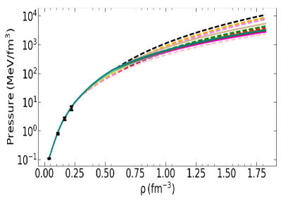
Figure 6.17: Pressure in $\beta$-stable matter as a function of density. The figure shows the spreading of the pressure values due to the matching of polytropes as explained in the text. Each curve is made up of the microscpic part (common to all cases) and twp polytropes with different adiabatic index, joined by smooth interpolation. The microscopic prediction are obtained at N³LO and cutoff equal to 450 MeV.

6.3.2   The TOV equations

With the EoS available over a full range of densities, we move to the mass–radius relation in a neutron star. In this section we will briefly review the relativistic equations for hydrostatic equilibrium, the TOV equations [320, 321] and how the mass–radius relationship emerges from them for a given input EoS. We will not go beyond the TOV equations to address, for instance, rotating stars, as our main purpose is to highlight the chief role of the EoS in the structure of neutron stars, which can be well demonstrated through static, cold stars.

The TOV equation describes a spherically symmetric inertial massive object composed of a perfect fluid in hydrostatic equilibrium. The equation relates the pressure within the star to the mass-energy density as functions of the radial distance from the star’s center:

$$\frac{dP(r)}{dr}=-\frac{G}{c^{2}}\ \frac{(P(r)+\epsilon(r))\ (M(r)+4\pi r^{3}\frac{P(r)}{c^{2}})}{r(r-\frac{2GM(r)}{c^{2}})}\;.$$ (6.39)

A spherical shell of material is related to the energy density at a distance $r$ from the star’s center by:

$$\frac{dM(r)}{dr}=\frac{4\pi}{c^{2}}r^{2}\epsilon(r)\;.$$ (6.40)

The star’s gravitational mass ($M$) is determined from the radius ($R$) and the mass-energy density ($\epsilon(r)$):

$$M(R)=\int^{R}_{0}\frac{\epsilon(r)}{c^{2}}\ d^{3}r\;.$$ (6.41)

Since the pressure and energy-density are functions of density, for a fixed central density the mass–radius of the star can be determined by Equations (6.40) and (6.39). Equation (6.39) can be integrated numerically by summing over shells of fixed width at incremented distance from the star’s center so as to evaluate the total pressure as a function of radial distance. Equation (6.40) can be integrated in the same fashion, simultaneously, to determine the mass contained within each spherical shell. To accomplish this, we employed the fourth-order Runge–Kutta method. The radial distance at which the pressure effectively vanishes corresponds to the star’s radius. Then, Equation (6.18) provides the total mass enclosed within such radius.

The $M(R)$ relation obtained from selected EoS extended with piecewise polytropes as explained above is shown in Fig. 6.18. We apply the constraint of causality and we only consider polytropes, which can support a maximum mass of at least 2.01 $M_{\odot}$, to be consistent with the lower limit of the (2.08 $\pm$ 0.07) $M_{\odot}$ observation reported in Ref. [370] for the J0740 + 6620 pulsar along with a radius estimate of (12.35 $\pm$ 0.75) km. Of the EoS that are consistent with the maximum mass constraints, some are causal up to and beyond the maximum mass, others are displayed up to the point where causality is violated. Of course, we must keep in mind that, at and near the central densities corresponding to the heavier stars, the EoS are polytropic and not the result of microscopic theory. What we do observe is that the best combination of polytropes, which satisfies both the maximum mass constraint and causality up and beyond the maximum mass, is given by a first polytrope with adiabatic index equal to about 3.0 - 3.2, joined to a second polytrope with lower adiabatic index, approximately 2.7 - 2.8. This scenario is consistent with a softening of the EoS at the highest densities.

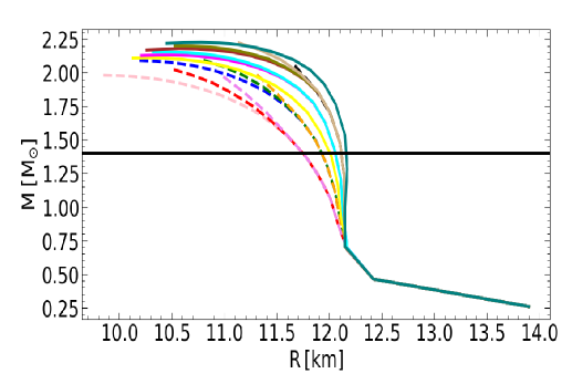
Figure 6.18: Mass-radius relation for a variety of EoS from Fig. 6.17. Each color/pattern corresponds to the same color/pattern in Fig. 6.17. Some curves are causal up and beyond the maximum mass, others are cut at the point where causality is violated. The horizontal line marks the 1.4 $M_{\odot}$ mass.

6.3.3   The radius of the average-mass neutron star

A fully microscopic EoS up to central densities of the most massive stars—potentially involving non-nucleonic degrees of freedom and phase transitions—is not within reach. Nevertheless, neutron stars are powerful natural laboratories for constraining theories of the EoS. One must be mindful about the theory’s limitations and the best ways to extract useful information from the observational constraints. Constraints on the radius of a medium-mass neutron star, $R_{1.4}$, are becoming more stringent, with the current uncertainty reported at about 2 km. Furthermore, $R_{1.4}$ is known to be sensitive to the pressure in neutron-rich matter near normal densities, accessible to modern effective field theories of nuclear forces. For these reasons, we focused on predicting $R_{1.4}$ with proper uncertainty quantification. Our neutron star calculations employing the EoS described in Sec. 6.2.1 and 6.2.2 are presented in detail in Ref. [285].

Using the tools reviewed above, our estimate of the radius for the canonical-mass neutron star can be stated as:

$$R_{1.4}=(11.96\pm 0.80)\;\mbox{km}\;,$$ (6.42)

in excellent agreement with the LIGO/Virgo range of 11.1 to 13.4 km [371].

Based on our analysis in Section 6.2.4, we are confident that the estimate given in Equation (6.42), approximately (12 $\pm$ 1) km, is characteristic of EFT predictions based on high-quality 2NF and properly calibrated (leading and subleading) 3NFs. The range currently cited for chiral EFT-based predictions of $R_{1.4}$ is between 10 km and 14 km, accounting for additional theoretical uncertainties. In fact, it is interesting to notice that the extensive analysis from Ref. [287], where 300,000 possible EoS were generated, provides a range for $R_{1.4}$ between 10.0 and 12.7 km, with 12.0 km being the most probable value. We recall that the outcome of PREX II gives 13.33 km as the lower limit for the radius, which is problematic to reconcile with a multitude of microscopic predictions [247].

Gravitational wave astronomy offers new exciting opportunities for nuclear astrophysics. Even though chiral EFT cannot reach out to the extreme-density and yet unknown regimes at the core of these remarkable stars, continuously improved ab initio calculations of the nuclear EoS are an essential foundation for interpreting current and future observations in terms of microscopic nuclear forces.

7   Conclusions

The past 20 years have seen great progress in our understanding of nuclear forces in terms of low-energy QCD. Key to this development was the realization that low-energy QCD is equivalent to an effective field theory (EFT) which has become known as chiral perturbation theory (ChPT) or chiral EFT. In fact, it can be argued that the chiral EFT approach to nuclear forces has considerable advantages over any earlier attempts, because chiral EFT

• is rooted in low-energy QCD;

• is, in principal, model-independent;

• occurs with an organizational scheme (‘power counting’) that allows to quantify the uncertainty of predictions;

• generates two- and many-body forces on an equal footing .

But the strength of chiral EFT extends beyond a purely formal level. Ab inito calculations applying chiral nuclear forces have been, in part, very successful. One example is the explanation of nuclear matter saturation. Though it was speculated early on that the addition of 3NFs might solve the problem, nonrelativistic calculations with phenomenological 3NFs failed to do so [143, 5, 147]. In contrast, the chiral 3NF at only leading order (NNLO) has the ability to solve that problem [110, 111, 112, 113, 114, 120]. The $N$-$d$ $A_{y}$ puzzle, which could never be resolved with phenomenological 3NFs [150], is another example for the success of EFT-based 3NFs [45].

Nevertheless problems remain. Just to mention one important issue: The simultaneous ab initio description of the bulk properties of medium-mass nuclei und nuclear matter saturation remains an outstanding challenge.

We have also reviewed the equations of state, for both SNM and pure NM, based upon chiral forces. We surveyed a large cross section of representative literature addressing the nuclear symmetry energy, with the objective to identify and discuss current gaps or problems, and provide recommendations for future research. There has been enormous progress in nuclear theory since the days of one-boson-exchange or phenomenological $NN$ potentials and phenomenological 3NFs, selected with no clear scheme or guidance. Predictions from state-of-the-art nuclear theory favor a softer density dependence of the symmetry energy – on the low-to-medium end of the spectrum found in the literature – and, naturally, smaller neutron skins and radii of canonical-mass neutron stars. To advance our understanding of these intriguing systems, it is important to build on that progress.

Last but not least, it needs to be pointed out that there are still problems at the foundation of the approach: Since EFT is a field theory, the standards to which it must measure up are higher than for a model. A sound EFT must be renormalizable and allow for a proper power counting (order-by-order arrangement). The presently used chiral nuclear potentials are based on naive dimensional analysis (‘Weinberg counting’) and apply a cutoff regularization scheme. In that scheme, one wishes to see cutoff independence of the results. Such independence is seen to a good degree below the breakdown scale [96, 111, 140], but to which extent that is satisfactory is controversial. The problem is due to the nonperturbative resummation necessary for typical nuclear physics problems (bound states). However, there is hope that from the current discussion [28, 67, 68, 69, 70, 71, 72, 73, 74, 75, 76, 77] constructive solutions may emerge [78, 79, 80].

In conclusion, considering both formal aspects and evidence of successful applications, one may say that chiral EFT has substantially advanced the field of theoretical nuclear physics [372]. But, at the same time, the community needs to be aware of the open challenges and work together building on the progress of the past 20 years.

References

- [1] R. B. Wiringa, V. G. J. Stoks, R. Schiavilla, An Accurate nucleon-nucleon potential with charge independence breaking, Phys. Rev. C 51 (1995) 38–51. arXiv:nucl-th/9408016, doi:10.1103/PhysRevC.51.38.
- [2] S. A. Coon, M. D. Scadron, P. C. McNamee, B. R. Barrett, D. W. E. Blatt, B. H. J. McKellar, The Two Pion Exchange, Three Nucleon Potential and Nuclear Matter, Nucl. Phys. A 317 (1979) 242–278. doi:10.1016/0375-9474(79)90462-7.
- [3] S. A. Coon, H. K. Han, Reworking the Tucson-Melbourne three nucleon potential, Few Body Syst. 30 (2001) 131–141. arXiv:nucl-th/0101003, doi:10.1007/s006010170022.
- [4] I. E. Lagaris, V. R. Pandharipande, Phenomenological two-nucleon interaction operator, Nucl. Phys. A 359 (1981) 331–348. doi:10.1016/0375-9474(81)90240-2.
- [5] J. Carlson, V. R. Pandharipande, R. B. Wiringa, Three-nucleon interaction in 3-body, 4-body, and infinite-body systems, Nucl. Phys. A 401 (1983) 59–85. doi:10.1016/0375-9474(83)90336-6.
- [6] B. S. Pudliner, V. R. Pandharipande, J. Carlson, R. B. Wiringa, Quantum Monte Carlo calculations of A = 6 nuclei, Phys. Rev. Lett. 74 (1995) 4396–4399. arXiv:nucl-th/9502031, doi:10.1103/PhysRevLett.74.4396.
- [7] H. Yukawa, On the Interaction of Elementary Particles I, Proc. Phys. Math. Soc. Jap. 17 (1935) 48–57. doi:10.1143/PTPS.1.1.
- [8] R. Bryan, B. L. Scott, Nucleon-nucleon scattering from one-boson-exchange potentials. iii. S-waves included, Phys. Rev. 177 (1969) 1435–1442. doi:10.1103/PhysRev.177.1435.
- [9] K. Erkelenz, Current status of the relativistic two-nucleon one-boson-exchange potential, Phys. Rept. 13 (1974) 191–258. doi:10.1016/0370-1573(74)90008-8.
- [10] K. Holinde, R. Machleidt, Momentum Space OBEP, Two-Nucleon and Nuclear Matter Data, Nucl. Phys. A 247 (1975) 495–520. doi:10.1016/0375-9474(75)90137-2.
- [11] R. Machleidt, The Meson theory of nuclear forces and nuclear structure, Adv. Nucl. Phys. 19 (1989) 189–376.
- [12] R. Machleidt, The high precision, charge-dependent Bonn nucleon-nucleon potential, Phys. Rev. C 63 (2001) 024001. arXiv:nucl-th/0006014, doi:10.1103/PhysRevC.63.024001.
- [13] M. Lacombe, B. Loiseau, J. M. Richard, R. Vinh Mau, J. Cote, P. Pires, R. De Tourreil, Parametrization of the Paris n n Potential, Phys. Rev. C 21 (1980) 861–873. doi:10.1103/PhysRevC.21.861.
- [14] R. Machleidt, K. Holinde, C. Elster, The Bonn Meson Exchange Model for the Nucleon Nucleon Interaction, Phys. Rept. 149 (1987) 1–89. doi:10.1016/S0370-1573(87)80002-9.
- [15] S. Aoki, T. Doi, Lattice QCD and baryon-baryon interactions: HAL QCD method, Front. in Phys. 8 (2020) 307. arXiv:2003.10730, doi:10.3389/fphy.2020.00307.
- [16] M. Illa, et al., Low-energy scattering and effective interactions of two baryons at MeV from lattice quantum chromodynamics, Phys. Rev. D 103 (5) (2021) 054508. arXiv:2009.12357, doi:10.1103/PhysRevD.103.054508.
- [17] S. Weinberg, Phenomenological Lagrangians, Physica A 96 (1-2) (1979) 327–340. doi:10.1016/0378-4371(79)90223-1.
- [18] S. Weinberg, Nuclear forces from chiral Lagrangians, Phys. Lett. B 251 (1990) 288–292. doi:10.1016/0370-2693(90)90938-3.
- [19] S. Weinberg, Effective chiral Lagrangians for nucleon - pion interactions and nuclear forces, Nucl. Phys. B 363 (1991) 3–18. doi:10.1016/0550-3213(91)90231-L.
- [20] J. Gasser, H. Leutwyler, Chiral Perturbation Theory to One Loop, Annals Phys. 158 (1984) 142. doi:10.1016/0003-4916(84)90242-2.
- [21] J. Gasser, H. Leutwyler, Chiral Perturbation Theory: Expansions in the Mass of the Strange Quark, Nucl. Phys. B 250 (1985) 465–516. doi:10.1016/0550-3213(85)90492-4.
- [22] J. Gasser, M. E. Sainio, A. Svarc, Nucleons with Chiral Loops, Nucl. Phys. B 307 (1988) 779–853. doi:10.1016/0550-3213(88)90108-3.
- [23] C. Ordonez, L. Ray, U. van Kolck, The Two nucleon potential from chiral Lagrangians, Phys. Rev. C 53 (1996) 2086–2105. arXiv:hep-ph/9511380, doi:10.1103/PhysRevC.53.2086.
- [24] S. Weinberg, Three body interactions among nucleons and pions, Phys. Lett. B 295 (1992) 114–121. arXiv:hep-ph/9209257, doi:10.1016/0370-2693(92)90099-P.
- [25] U. van Kolck, Few nucleon forces from chiral Lagrangians, Phys. Rev. C 49 (1994) 2932–2941. doi:10.1103/PhysRevC.49.2932.
- [26] R. Machleidt, D. R. Entem, Chiral effective field theory and nuclear forces, Phys. Rept. 503 (2011) 1–75. arXiv:1105.2919, doi:10.1016/j.physrep.2011.02.001.
- [27] E. Epelbaum, H.-W. Hammer, U.-G. Meissner, Modern Theory of Nuclear Forces, Rev. Mod. Phys. 81 (2009) 1773–1825. arXiv:0811.1338, doi:10.1103/RevModPhys.81.1773.
- [28] H. W. Hammer, S. König, U. van Kolck, Nuclear effective field theory: status and perspectives, Rev. Mod. Phys. 92 (2) (2020) 025004. arXiv:1906.12122, doi:10.1103/RevModPhys.92.025004.
- [29] E. Jenkins, A. V. Manohar, Baryon chiral perturbation theory using a heavy fermion lagrangian, Phys. Lett. B 255 (1991) 558.
- [30] H. Krebs, A. Gasparyan, E. Epelbaum, Chiral three-nucleon force at N4LO I: Longest-range contributions, Phys. Rev. C 85 (2012) 054006. arXiv:1203.0067, doi:10.1103/PhysRevC.85.054006.
- [31] R. J. Furnstahl, N. Klco, D. R. Phillips, S. Wesolowski, Quantifying truncation errors in effective field theory, Phys. Rev. C 92 (2) (2015) 024005. arXiv:1506.01343, doi:10.1103/PhysRevC.92.024005.
- [32] E. Epelbaum, Four-nucleon force in chiral effective field theory, Phys. Lett. B 639 (2006) 456–461. arXiv:nucl-th/0511025, doi:10.1016/j.physletb.2006.06.046.
- [33] R. L. Workman, et al., Review of Particle Physics, PTEP 2022 (2022) 083C01. doi:10.1093/ptep/ptac097.
- [34] N. Kaiser, R. Brockmann, W. Weise, Peripheral nucleon-nucleon phase shifts and chiral symmetry, Nucl. Phys. A 625 (1997) 758–788. arXiv:nucl-th/9706045, doi:10.1016/S0375-9474(97)00586-1.
- [35] E. Epelbaum, A. Nogga, W. Gloeckle, H. Kamada, U. G. Meissner, H. Witala, Three nucleon forces from chiral effective field theory, Phys. Rev. C 66 (2002) 064001. arXiv:nucl-th/0208023, doi:10.1103/PhysRevC.66.064001.
- [36] N. Kaiser, Chiral 3 pi exchange N N potentials: Results for representation invariant classes of diagrams, Phys. Rev. C 61 (2000) 014003. arXiv:nucl-th/9910044, doi:10.1103/PhysRevC.61.014003.
- [37] N. Kaiser, Chiral three pi exchange N N potentials: Results for diagrams proportional to g(A)**4 and g(A)**6, Phys. Rev. C 62 (2000) 024001. arXiv:nucl-th/9912054, doi:10.1103/PhysRevC.62.024001.
- [38] D. R. Entem, R. Machleidt, Accurate charge dependent nucleon nucleon potential at fourth order of chiral perturbation theory, Phys. Rev. C 68 (2003) 041001. arXiv:nucl-th/0304018, doi:10.1103/PhysRevC.68.041001.
- [39] V. Bernard, E. Epelbaum, H. Krebs, U.-G. Meissner, Subleading contributions to the chiral three-nucleon force. I. Long-range terms, Phys. Rev. C 77 (2008) 064004. arXiv:0712.1967, doi:10.1103/PhysRevC.77.064004.
- [40] V. Bernard, E. Epelbaum, H. Krebs, U. G. Meissner, Subleading contributions to the chiral three-nucleon force II: Short-range terms and relativistic corrections, Phys. Rev. C 84 (2011) 054001. arXiv:1108.3816, doi:10.1103/PhysRevC.84.054001.
- [41] E. Epelbaum, Four-nucleon force using the method of unitary transformation, Eur. Phys. J. A 34 (2007) 197–214. arXiv:0710.4250, doi:10.1140/epja/i2007-10496-0.
- [42] D. R. Entem, N. Kaiser, R. Machleidt, Y. Nosyk, Peripheral nucleon-nucleon scattering at fifth order of chiral perturbation theory, Phys. Rev. C 91 (1) (2015) 014002. arXiv:1411.5335, doi:10.1103/PhysRevC.91.014002.
- [43] H. Krebs, A. Gasparyan, E. Epelbaum, Chiral three-nucleon force at II: Intermediate-range contributions, Phys. Rev. C 87 (5) (2013) 054007. arXiv:1302.2872, doi:10.1103/PhysRevC.87.054007.
- [44] L. Girlanda, A. Kievsky, M. Viviani, Subleading contributions to the three-nucleon contact interaction, Phys. Rev. C 84 (1) (2011) 014001, [Erratum: Phys.Rev.C 102, 019903 (2020)]. arXiv:1102.4799, doi:10.1103/PhysRevC.84.014001.
- [45] L. Girlanda, A. Kievsky, M. Viviani, L. E. Marcucci, Short-range three-nucleon interaction from A=3 data and its hierarchical structure, Phys. Rev. C 99 (5) (2019) 054003. arXiv:1811.09398, doi:10.1103/PhysRevC.99.054003.
- [46] D. R. Entem, N. Kaiser, R. Machleidt, Y. Nosyk, Dominant contributions to the nucleon-nucleon interaction at sixth order of chiral perturbation theory, Phys. Rev. C 92 (6) (2015) 064001. arXiv:1505.03562, doi:10.1103/PhysRevC.92.064001.
- [47] D. R. Entem, R. Machleidt, Contact terms up to sixth order, unpublished.
- [48] V. G. J. Stoks, R. A. M. Klomp, M. C. M. Rentmeester, J. J. de Swart, Partial wave analaysis of all nucleon-nucleon scattering data below 350-MeV, Phys. Rev. C 48 (1993) 792–815. doi:10.1103/PhysRevC.48.792.
- [49] R. A. Arndt, W. J. Briscoe, I. I. Strakovsky, R. L. Workman, Updated analysis of NN elastic scattering to 3-GeV, Phys. Rev. C 76 (2007) 025209. arXiv:0706.2195, doi:10.1103/PhysRevC.76.025209.
- [50] D. R. Entem, R. Machleidt, Accurate nucleon-nucleon potential based upon chiral perturbation theory, Phys. Lett. B 524 (2002) 93–98. arXiv:nucl-th/0108057, doi:10.1016/S0370-2693(01)01363-6.
- [51] R. Vinh Mau, The Paris Nucleon-Nucleon Potential, in: M. Rho, D. H. Wilkinson (Eds.), Mesons in Nuclei, Vol. I, North-Holland, Amsterdam (1979) pp. 151–196.
- [52] M. Hoferichter, J. Ruiz de Elvira, B. Kubis, U.-G. Meißner, Matching pion-nucleon Roy-Steiner equations to chiral perturbation theory, Phys. Rev. Lett. 115 (19) (2015) 192301. arXiv:1507.07552, doi:10.1103/PhysRevLett.115.192301.
- [53] M. Hoferichter, J. Ruiz de Elvira, B. Kubis, U.-G. Meißner, Roy–Steiner-equation analysis of pion–nucleon scattering, Phys. Rept. 625 (2016) 1–88. arXiv:1510.06039, doi:10.1016/j.physrep.2016.02.002.
- [54] D. Siemens, J. Ruiz de Elvira, E. Epelbaum, M. Hoferichter, H. Krebs, B. Kubis, U. G. Meißner, Reconciling threshold and subthreshold expansions for pion–nucleon scattering, Phys. Lett. B 770 (2017) 27–34. arXiv:1610.08978, doi:10.1016/j.physletb.2017.04.039.
- [55] K. Holinde, R. Machleidt, Effect of the Delta (1236) Resonance on n n Scattering, Nuclear Matter and Neutron Matter, Nucl. Phys. A 280 (1977) 429–466. doi:10.1016/0375-9474(77)90614-5.
- [56] T. R. Hemmert, B. R. Holstein, J. Kambor, Chiral Lagrangians and Delta(1232) interactions: Formalism, J. Phys. G 24 (1998) 1831–1859. arXiv:hep-ph/9712496, doi:10.1088/0954-3899/24/10/003.
- [57] V. Bernard, N. Kaiser, U.-G. Meissner, Aspects of chiral pion - nucleon physics, Nucl. Phys. A 615 (1997) 483–500. arXiv:hep-ph/9611253, doi:10.1016/S0375-9474(97)00021-3.
- [58] N. Kaiser, S. Gerstendorfer, W. Weise, Peripheral NN scattering: Role of delta excitation, correlated two pion and vector meson exchange, Nucl. Phys. A 637 (1998) 395–420. arXiv:nucl-th/9802071, doi:10.1016/S0375-9474(98)00234-6.
- [59] H. Krebs, E. Epelbaum, U.-G. Meissner, Nuclear forces with Delta-excitations up to next-to-next-to-leading order. I. Peripheral nucleon-nucleon waves, Eur. Phys. J. A 32 (2007) 127–137. arXiv:nucl-th/0703087, doi:10.1140/epja/i2007-10372-y.
- [60] E. Epelbaum, H. Krebs, U.-G. Meissner, Delta-excitations and the three-nucleon force, Nucl. Phys. A 806 (2008) 65–78. arXiv:0712.1969, doi:10.1016/j.nuclphysa.2008.02.305.
- [61] H. Krebs, A. M. Gasparyan, E. Epelbaum, Three-nucleon force in chiral EFT with explicit degrees of freedom: Longest-range contributions at fourth order, Phys. Rev. C 98 (1) (2018) 014003. arXiv:1803.09613, doi:10.1103/PhysRevC.98.014003.
- [62] Y. Nosyk, D. R. Entem, R. Machleidt, Nucleon-nucleon potentials from -full chiral effective-field-theory and implications, Phys. Rev. C 104 (5) (2021) 054001. arXiv:2107.06452, doi:10.1103/PhysRevC.104.054001.
- [63] S. C. Pieper, V. R. Pandharipande, R. B. Wiringa, J. Carlson, Realistic models of pion exchange three nucleon interactions, Phys. Rev. C 64 (2001) 014001. arXiv:nucl-th/0102004, doi:10.1103/PhysRevC.64.014001.
- [64] E. Epelbaum, U.-G. Meissner, W. Glöeckle, C. Elster, Resonance saturation for four-nucleon operators, Phys. Rev. C 65 (2002) 044001.
- [65] D. B. Kaplan, M. J. Savage, M. B. Wise, Nucleon - nucleon scattering from effective field theory, Nucl. Phys. B 478 (1996) 629–659. arXiv:nucl-th/9605002, doi:10.1016/0550-3213(96)00357-4.
- [66] S. Fleming, T. Mehen, I. W. Stewart, NNLO corrections to nucleon-nucleon scattering and perturbative pions, Nucl. Phys. A 677 (2000) 313–366. arXiv:nucl-th/9911001, doi:10.1016/S0375-9474(00)00221-9.
- [67] A. Nogga, R. G. E. Timmermans, U. van Kolck, Renormalization of one-pion exchange and power counting, Phys. Rev. C 72 (2005) 054006. arXiv:nucl-th/0506005, doi:10.1103/PhysRevC.72.054006.
- [68] M. C. Birse, Power counting with one-pion exchange, Phys. Rev. C 74 (2006) 014003. arXiv:nucl-th/0507077, doi:10.1103/PhysRevC.74.014003.
- [69] B. Long, C. J. Yang, Short-range nuclear forces in singlet channels, Phys. Rev. C 86 (2012) 024001. arXiv:1202.4053, doi:10.1103/PhysRevC.86.024001.
- [70] B. Long, Power counting for nuclear forces in chiral effective field theory, Int. J. Mod. Phys. E 25 (05) (2016) 1641006. arXiv:1603.01002, doi:10.1142/S0218301316410068.
- [71] M. P. Valderrama, Perturbative renormalizability of chiral two pion exchange in nucleon-nucleon scattering, Phys. Rev. C 83 (2011) 024003. arXiv:0912.0699, doi:10.1103/PhysRevC.83.024003.
- [72] M. Pavon Valderrama, Perturbative Renormalizability of Chiral Two Pion Exchange in Nucleon-Nucleon Scattering: P- and D-waves, Phys. Rev. C 84 (2011) 064002. arXiv:1108.0872, doi:10.1103/PhysRevC.84.064002.
- [73] M. P. Valderrama, Power Counting and Wilsonian Renormalization in Nuclear Effective Field Theory, Int. J. Mod. Phys. E 25 (05) (2016) 1641007. arXiv:1604.01332, doi:10.1142/S021830131641007X.
- [74] M. Pavón Valderrama, M. Sánchez Sánchez, C. J. Yang, B. Long, J. Carbonell, U. van Kolck, Power Counting in Peripheral Partial Waves: The Singlet Channels, Phys. Rev. C 95 (5) (2017) 054001. arXiv:1611.10175, doi:10.1103/PhysRevC.95.054001.
- [75] E. Epelbaum, J. Gegelia, U.-G. Meißner, Wilsonian renormalization group versus subtractive renormalization in effective field theories for nucleon–nucleon scattering, Nucl. Phys. B 925 (2017) 161–185. arXiv:1705.02524, doi:10.1016/j.nuclphysb.2017.10.008.
- [76] S. König, H. W. Grießhammer, H. W. Hammer, U. van Kolck, Nuclear Physics Around the Unitarity Limit, Phys. Rev. Lett. 118 (20) (2017) 202501. arXiv:1607.04623, doi:10.1103/PhysRevLett.118.202501.
- [77] E. Epelbaum, A. M. Gasparyan, J. Gegelia, U.-G. Meißner, How (not) to renormalize integral equations with singular potentials in effective field theory, Eur. Phys. J. A 54 (11) (2018) 186. arXiv:1810.02646, doi:10.1140/epja/i2018-12632-1.
- [78] U. van Kolck, The Problem of Renormalization of Chiral Nuclear Forces, Front. in Phys. 8 (2020) 79. arXiv:2003.06721, doi:10.3389/fphy.2020.00079.
-
[79]
M. Pavon Valderrama, Scattering amplitudes versus potentials in nuclear
effective field theory: is there a potential compromise?
arXiv:1902.08172. - [80] D. R. Entem, J. A. Oller, Non-perturbative methods for NN singular interactions, Eur. Phys. J. ST 230 (6) (2021) 1675–1689. arXiv:2103.02069, doi:10.1140/epjs/s11734-021-00149-2.
- [81] E. Epelbaum, W. Gloeckle, U.-G. Meissner, Nuclear forces from chiral Lagrangians using the method of unitary transformation. 2. The two nucleon system, Nucl. Phys. A 671 (2000) 295–331. arXiv:nucl-th/9910064, doi:10.1016/S0375-9474(99)00821-0.
- [82] E. Epelbaum, W. Glockle, U.-G. Meissner, The Two-nucleon system at next-to-next-to-next-to-leading order, Nucl. Phys. A 747 (2005) 362–424. arXiv:nucl-th/0405048, doi:10.1016/j.nuclphysa.2004.09.107.
- [83] E. Epelbaum, H. Krebs, U. G. Meißner, Improved chiral nucleon-nucleon potential up to next-to-next-to-next-to-leading order, Eur. Phys. J. A 51 (5) (2015) 53. arXiv:1412.0142, doi:10.1140/epja/i2015-15053-8.
- [84] E. Epelbaum, H. Krebs, U. G. Meißner, Precision nucleon-nucleon potential at fifth order in the chiral expansion, Phys. Rev. Lett. 115 (12) (2015) 122301. arXiv:1412.4623, doi:10.1103/PhysRevLett.115.122301.
- [85] A. Ekström, et al., Optimized Chiral Nucleon-Nucleon Interaction at Next-to-Next-to-Leading Order, Phys. Rev. Lett. 110 (19) (2013) 192502. arXiv:1303.4674, doi:10.1103/PhysRevLett.110.192502.
- [86] A. Gezerlis, I. Tews, E. Epelbaum, M. Freunek, S. Gandolfi, K. Hebeler, A. Nogga, A. Schwenk, Local chiral effective field theory interactions and quantum Monte Carlo applications, Phys. Rev. C 90 (5) (2014) 054323. arXiv:1406.0454, doi:10.1103/PhysRevC.90.054323.
- [87] M. Piarulli, L. Girlanda, R. Schiavilla, R. Navarro Pérez, J. E. Amaro, E. Ruiz Arriola, Minimally nonlocal nucleon-nucleon potentials with chiral two-pion exchange including resonances, Phys. Rev. C 91 (2) (2015) 024003. arXiv:1412.6446, doi:10.1103/PhysRevC.91.024003.
- [88] M. Piarulli, L. Girlanda, R. Schiavilla, A. Kievsky, A. Lovato, L. E. Marcucci, S. C. Pieper, M. Viviani, R. B. Wiringa, Local chiral potentials with -intermediate states and the structure of light nuclei, Phys. Rev. C 94 (5) (2016) 054007. arXiv:1606.06335, doi:10.1103/PhysRevC.94.054007.
- [89] R. Navarro Pérez, J. E. Amaro, E. Ruiz Arriola, Low energy chiral two pion exchange potential with statistical uncertainties, Phys. Rev. C 91 (5) (2015) 054002. arXiv:1411.1212, doi:10.1103/PhysRevC.91.054002.
- [90] B. D. Carlsson, A. Ekström, C. Forssén, D. F. Strömberg, G. R. Jansen, O. Lilja, M. Lindby, B. A. Mattsson, K. A. Wendt, Uncertainty analysis and order-by-order optimization of chiral nuclear interactions, Phys. Rev. X 6 (1) (2016) 011019. arXiv:1506.02466, doi:10.1103/PhysRevX.6.011019.
- [91] P. Reinert, H. Krebs, E. Epelbaum, Semilocal momentum-space regularized chiral two-nucleon potentials up to fifth order, Eur. Phys. J. A 54 (5) (2018) 86. arXiv:1711.08821, doi:10.1140/epja/i2018-12516-4.
- [92] A. Ekström, G. R. Jansen, K. A. Wendt, G. Hagen, T. Papenbrock, B. D. Carlsson, C. Forssén, M. Hjorth-Jensen, P. Navrátil, W. Nazarewicz, Accurate nuclear radii and binding energies from a chiral interaction, Phys. Rev. C 91 (5) (2015) 051301. arXiv:1502.04682, doi:10.1103/PhysRevC.91.051301.
- [93] A. Ekström, G. Hagen, T. D. Morris, T. Papenbrock, P. D. Schwartz, isobars and nuclear saturation, Phys. Rev. C 97 (2) (2018) 024332. arXiv:1707.09028, doi:10.1103/PhysRevC.97.024332.
- [94] D. R. Entem, R. Machleidt, Y. Nosyk, High-quality two-nucleon potentials up to fifth order of the chiral expansion, Phys. Rev. C 96 (2) (2017) 024004. arXiv:1703.05454, doi:10.1103/PhysRevC.96.024004.
-
[95]
G. P. Lepage, How to renormalize the Schrodinger equation, in: 8th Jorge
Andre Swieca Summer School on Nuclear Physics.
, 1997, pp. 135–180. arXiv:nucl-th/9706029. - [96] E. Marji, A. Canul, Q. MacPherson, R. Winzer, C. Zeoli, D. R. Entem, R. Machleidt, Nonperturbative renormalization of the chiral nucleon-nucleon interaction up to next-to-next-to-leading order, Phys. Rev. C 88 (5) (2013) 054002. arXiv:1309.5114, doi:10.1103/PhysRevC.88.054002.
- [97] R. Blankenbecler, R. Sugar, Linear integral equations for relativistic multichannel scattering, Phys. Rev. 142 (1966) 1051–1059. doi:10.1103/PhysRev.142.1051.
- [98] W. G. Jiang, A. Ekström, C. Forssén, G. Hagen, G. R. Jansen, T. Papenbrock, Accurate bulk properties of nuclei from to from potentials with isobars, Phys. Rev. C 102 (5) (2020) 054301. arXiv:2006.16774, doi:10.1103/PhysRevC.102.054301.
- [99] S. K. Saha, D. R. Entem, R. Machleidt, Y. Nosyk, Local position-space two-nucleon potentials from leading to fourth order of chiral effective field theory, Phys. Rev. C 107 (3) (2023) 034002. arXiv:2209.13170, doi:10.1103/PhysRevC.107.034002.
- [100] R. Somasundaram, J. E. Lynn, L. Huth, A. Schwenk, I. Tews, Maximally local two-nucleon interactions at fourth order in delta-less chiral effective field theoryarXiv:2306.13579.
- [101] J. Carlson, S. Gandolfi, F. Pederiva, S. C. Pieper, R. Schiavilla, K. E. Schmidt, R. B. Wiringa, Quantum Monte Carlo methods for nuclear physics, Rev. Mod. Phys. 87 (2015) 1067. arXiv:1412.3081, doi:10.1103/RevModPhys.87.1067.
- [102] J. E. Lynn, I. Tews, S. Gandolfi, A. Lovato, Quantum Monte Carlo Methods in Nuclear Physics: Recent Advances, Ann. Rev. Nucl. Part. Sci. 69 (2019) 279–305. arXiv:1901.04868, doi:10.1146/annurev-nucl-101918-023600.
- [103] M. Piarulli, I. Tews, Local Nucleon-Nucleon and Three-Nucleon Interactions Within Chiral Effective Field Theory, Front. in Phys. 7 (2020) 245. arXiv:2002.00032, doi:10.3389/fphy.2019.00245.
- [104] S. Okubo, R. E. Marshak, Velocity dependence of the two-nucleon interaction, Annals Phys. 4 (2) (1958) 166–179. doi:10.1016/0003-4916(58)90031-9.
- [105] L. Huth, I. Tews, J. E. Lynn, A. Schwenk, Analyzing the Fierz Rearrangement Freedom for Local Chiral Two-Nucleon Potentials, Phys. Rev. C 96 (5) (2017) 054003. arXiv:1708.03194, doi:10.1103/PhysRevC.96.054003.
- [106] U. D. Jentschura, A. Matveev, C. G. Parthey, J. Alnis, R. Pohl, T. Udem, N. Kolachevsky, T. W. Ha̋nsch, Hydrogen-deuterium isotope shift: From the 1S-2S-transition frequency to the proton-deuteron charge-radius difference, Phys Rev. A 83 (2011) 042505.
-
[107]
E. Epelbaum, H. Krebs, P. Reinert, Semi-local nuclear forces from chiral EFT:
State-of-the-art and challenges.
arXiv:2206.07072. - [108] D. R. Entem, R. Machleidt, H. Witala, Chiral NN model and A(y) puzzle, Phys. Rev. C 65 (2002) 064005. arXiv:nucl-th/0111033, doi:10.1103/PhysRevC.65.064005.
- [109] E. Caurier, P. Navrátil, W. E. Ormand, J. P. Vary, Ab initio shell model for A=10 nuclei, Phys. Rev. C 66 (2002) 024314. doi:10.1103/PhysRevC.66.024314.
- [110] F. Sammarruca, B. Chen, L. Coraggio, N. Itaco, R. Machleidt, Dirac-Brueckner-Hartree-Fock versus chiral effective field theory, Phys. Rev. C 86 (2012) 054317. arXiv:1209.5001, doi:10.1103/PhysRevC.86.054317.
- [111] L. Coraggio, J. W. Holt, N. Itaco, R. Machleidt, L. E. Marcucci, F. Sammarruca, Nuclear-matter equation of state with consistent two- and three-body perturbative chiral interactions, Phys. Rev. C 89 (4) (2014) 044321. arXiv:1402.0965, doi:10.1103/PhysRevC.89.044321.
- [112] F. Sammarruca, L. Coraggio, J. W. Holt, N. Itaco, R. Machleidt, L. E. Marcucci, Toward order-by-order calculations of the nuclear and neutron matter equations of state in chiral effective field theory, Phys. Rev. C 91 (5) (2015) 054311. arXiv:1411.0136, doi:10.1103/PhysRevC.91.054311.
- [113] R. Machleidt, F. Sammarruca, Chiral EFT based nuclear forces: Achievements and challenges, Phys. Scripta 91 (8) (2016) 083007. arXiv:1608.05978, doi:10.1088/0031-8949/91/8/083007.
-
[114]
F. Sammarruca, L. E. Marcucci, L. Coraggio, J. W. Holt, N. Itaco, R. Machleidt,
Nuclear and neutron matter equations of state from high-quality potentials
up to fifth order of the chiral expansion.
arXiv:1807.06640. - [115] K. Hebeler, Three-nucleon forces: Implementation and applications to atomic nuclei and dense matter, Phys. Rept. 890 (2021) 1–116. arXiv:2002.09548, doi:10.1016/j.physrep.2020.08.009.
- [116] J. Fujita, H. Miyazawa, Pion Theory of Three-Body Forces, Prog. Theor. Phys. 17 (1957) 360–365. doi:10.1143/PTP.17.360.
- [117] J. L. Friar, D. Huber, U. van Kolck, Chiral symmetry and three nucleon forces, Phys. Rev. C 59 (1999) 53–58. arXiv:nucl-th/9809065, doi:10.1103/PhysRevC.59.53.
- [118] P. Navrátil, Local three-nucleon interaction from chiral effective field theory, Few Body Syst. 41 (2007) 117–140. arXiv:0707.4680, doi:10.1007/s00601-007-0193-3.
- [119] A. Nogga, P. Navrátil, B. R. Barrett, J. P. Vary, Spectra and binding energy predictions of chiral interactions for Li-7, Phys. Rev. C 73 (2006) 064002. arXiv:nucl-th/0511082, doi:10.1103/PhysRevC.73.064002.
- [120] K. Hebeler, S. K. Bogner, R. J. Furnstahl, A. Nogga, A. Schwenk, Improved nuclear matter calculations from chiral low-momentum interactions, Phys. Rev. C 83 (2011) 031301. arXiv:1012.3381, doi:10.1103/PhysRevC.83.031301.
- [121] L. E. Marcucci, A. Kievsky, S. Rosati, R. Schiavilla, M. Viviani, Chiral effective field theory predictions for muon capture on deuteron and , Phys. Rev. Lett. 108 (2012) 052502, [Erratum: Phys.Rev.Lett. 121, 049901 (2018)]. arXiv:1109.5563, doi:10.1103/PhysRevLett.108.052502.
- [122] P. Navrátil, R. Roth, S. Quaglioni, Ab initio many-body calculations of nucleon scattering on O, Phys. Rev. C 82 (2010) 034609. arXiv:1007.0525, doi:10.1103/PhysRevC.82.034609.
- [123] M. Viviani, L. Girlanda, A. Kievsky, L. E. Marcucci, Effect of three-nucleon interaction in p-3He elastic scattering, Phys. Rev. Lett. 111 (2013) 172302. arXiv:1307.5167, doi:10.1103/PhysRevLett.111.172302.
- [124] P. Navrátil, V. G. Gueorguiev, J. P. Vary, W. E. Ormand, A. Nogga, Structure of A=10-13 nuclei with two plus three-nucleon interactions from chiral effective field theory, Phys. Rev. Lett. 99 (2007) 042501. arXiv:nucl-th/0701038, doi:10.1103/PhysRevLett.99.042501.
- [125] R. Roth, J. Langhammer, A. Calci, S. Binder, P. Navrátil, Similarity-Transformed Chiral NN+3N Interactions for the Ab Initio Description of 12-C and 16-O, Phys. Rev. Lett. 107 (2011) 072501. arXiv:1105.3173, doi:10.1103/PhysRevLett.107.072501.
- [126] R. Roth, S. Binder, K. Vobig, A. Calci, J. Langhammer, P. Navrátil, Ab Initio Calculations of Medium-Mass Nuclei with Normal-Ordered Chiral NN+3N Interactions, Phys. Rev. Lett. 109 (2012) 052501. arXiv:1112.0287, doi:10.1103/PhysRevLett.109.052501.
- [127] G. Hagen, M. Hjorth-Jensen, G. R. Jansen, R. Machleidt, T. Papenbrock, Continuum effects and three-nucleon forces in neutron-rich oxygen isotopes, Phys. Rev. Lett. 108 (2012) 242501. arXiv:1202.2839, doi:10.1103/PhysRevLett.108.242501.
- [128] G. Hagen, M. Hjorth-Jensen, G. R. Jansen, R. Machleidt, T. Papenbrock, Evolution of shell structure in neutron-rich calcium isotopes, Phys. Rev. Lett. 109 (2012) 032502. arXiv:1204.3612, doi:10.1103/PhysRevLett.109.032502.
- [129] B. R. Barrett, P. Navrátil, J. P. Vary, Ab initio no core shell model, Prog. Part. Nucl. Phys. 69 (2013) 131–181. doi:10.1016/j.ppnp.2012.10.003.
- [130] H. Hergert, S. K. Bogner, S. Binder, A. Calci, J. Langhammer, R. Roth, A. Schwenk, In-Medium Similarity Renormalization Group with Chiral Two- Plus Three-Nucleon Interactions, Phys. Rev. C 87 (3) (2013) 034307. arXiv:1212.1190, doi:10.1103/PhysRevC.87.034307.
- [131] G. Hagen, T. Papenbrock, M. Hjorth-Jensen, D. J. Dean, Coupled-cluster computations of atomic nuclei, Rept. Prog. Phys. 77 (9) (2014) 096302. arXiv:1312.7872, doi:10.1088/0034-4885/77/9/096302.
- [132] S. Binder, J. Langhammer, A. Calci, R. Roth, Ab Initio Path to Heavy Nuclei, Phys. Lett. B 736 (2014) 119–123. arXiv:1312.5685, doi:10.1016/j.physletb.2014.07.010.
- [133] G. Hagen, G. R. Jansen, T. Papenbrock, Structure of 78Ni from first principles computations, Phys. Rev. Lett. 117 (17) (2016) 172501. arXiv:1605.01477, doi:10.1103/PhysRevLett.117.172501.
- [134] J. Simonis, K. Hebeler, J. D. Holt, J. Menendez, A. Schwenk, Exploring sd-shell nuclei from two- and three-nucleon interactions with realistic saturation properties, Phys. Rev. C 93 (1) (2016) 011302. arXiv:1508.05040, doi:10.1103/PhysRevC.93.011302.
- [135] J. Simonis, S. R. Stroberg, K. Hebeler, J. D. Holt, A. Schwenk, Saturation with chiral interactions and consequences for finite nuclei, Phys. Rev. C 96 (1) (2017) 014303. arXiv:1704.02915, doi:10.1103/PhysRevC.96.014303.
- [136] T. D. Morris, J. Simonis, S. R. Stroberg, C. Stumpf, G. Hagen, J. D. Holt, G. R. Jansen, T. Papenbrock, R. Roth, A. Schwenk, Structure of the lightest tin isotopes, Phys. Rev. Lett. 120 (15) (2018) 152503. arXiv:1709.02786, doi:10.1103/PhysRevLett.120.152503.
- [137] V. Somà, P. Navrátil, F. Raimondi, C. Barbieri, T. Duguet, Novel chiral Hamiltonian and observables in light and medium-mass nuclei, Phys. Rev. C 101 (1) (2020) 014318. arXiv:1907.09790, doi:10.1103/PhysRevC.101.014318.
- [138] K. Hebeler, A. Schwenk, Chiral three-nucleon forces and neutron matter, Phys. Rev. C 82 (2010) 014314. arXiv:0911.0483, doi:10.1103/PhysRevC.82.014314.
- [139] G. Hagen, T. Papenbrock, A. Ekström, K. A. Wendt, G. Baardsen, S. Gandolfi, M. Hjorth-Jensen, C. J. Horowitz, Coupled-cluster calculations of nucleonic matter, Phys. Rev. C 89 (1) (2014) 014319. arXiv:1311.2925, doi:10.1103/PhysRevC.89.014319.
- [140] L. Coraggio, J. W. Holt, N. Itaco, R. Machleidt, F. Sammarruca, Reduced regulator dependence of neutron-matter predictions with perturbative chiral interactions, Phys. Rev. C 87 (1) (2013) 014322. arXiv:1209.5537, doi:10.1103/PhysRevC.87.014322.
- [141] J. W. Negele, Structure of Finite Nuclei in the Local-Density Approximation, Phys. Rev. C 1 (1970) 1260–1321. doi:10.1103/PhysRevC.1.1260.
- [142] F. Coester, S. Cohen, B. Day, C. M. Vincent, Variation in Nuclear-Matter Binding Energies with Phase-Shift-Equivalent Two-Body Potentials, Phys. Rev. C 1 (1970) 769–776. doi:10.1103/PhysRevC.1.769.
- [143] B. D. Day, Nuclear Saturation and Nuclear Forces, Comments Nucl. Part. Phys. 11 (3) (1983) 115–126.
- [144] R. A. Brandenburg, Y. E. Kim, A. Tubis, Trinucleon Properties from a Complete Solution of the Faddeev Equations with the Reid Soft Core Potential, Phys. Lett. B 49 (1974) 205–208. doi:10.1016/0370-2693(74)90413-4.
- [145] R. A. Brandenburg, P. U. Sauer, R. Machleidt, Trinucleon Properties with One Boson Exchange Potentials, Z. Physik A 280 (1977) 93–97.
- [146] S. C. Pieper, The Illinois Extension to the Fujita-Miyazawa Three-Nucleon Force, AIP Conf. Proc. 1011 (1) (2008) 143–152. doi:10.1063/1.2932280.
- [147] A. Akmal, V. R. Pandharipande, D. G. Ravenhall, The Equation of state of nucleon matter and neutron star structure, Phys. Rev. C 58 (1998) 1804–1828. arXiv:nucl-th/9804027, doi:10.1103/PhysRevC.58.1804.
- [148] D. Lonardoni, A. Lovato, S. C. Pieper, R. B. Wiringa, Variational calculation of the ground state of closed-shell nuclei up to , Phys. Rev. C 96 (2) (2017) 024326. arXiv:1705.04337, doi:10.1103/PhysRevC.96.024326.
- [149] P. Maris, J. P. Vary, S. Gandolfi, J. Carlson, S. C. Pieper, Properties of trapped neutrons interacting with realistic nuclear Hamiltonians, Phys. Rev. C 87 (5) (2013) 054318. arXiv:1302.2089, doi:10.1103/PhysRevC.87.054318.
- [150] A. Kievsky, M. Viviani, L. Girlanda, L. E. Marcucci, Comparative study of three-nucleon force models in systems, Phys. Rev. C 81 (2010) 044003. arXiv:1002.1601, doi:10.1103/PhysRevC.81.044003.
- [151] J. Golak, et al., Low-energy neutron-deuteron reactions with N3LO chiral forces, Eur. Phys. J. A 50 (2014) 177. arXiv:1410.0756, doi:10.1140/epja/i2014-14177-7.
- [152] T. Krüger, I. Tews, K. Hebeler, A. Schwenk, Neutron matter from chiral effective field theory interactions, Phys. Rev. C 88 (2013) 025802. arXiv:1304.2212, doi:10.1103/PhysRevC.88.025802.
- [153] C. Drischler, A. Carbone, K. Hebeler, A. Schwenk, Neutron matter from chiral two- and three-nucleon calculations up to N3LO, Phys. Rev. C 94 (5) (2016) 054307. arXiv:1608.05615, doi:10.1103/PhysRevC.94.054307.
- [154] K. Hebeler, H. Krebs, E. Epelbaum, J. Golak, R. Skibinski, Efficient calculation of chiral three-nucleon forces up to N3LO for ab initio studies, Phys. Rev. C 91 (4) (2015) 044001. arXiv:1502.02977, doi:10.1103/PhysRevC.91.044001.
- [155] C. Drischler, K. Hebeler, A. Schwenk, Chiral interactions up to next-to-next-to-next-to-leading order and nuclear saturation, Phys. Rev. Lett. 122 (4) (2019) 042501. arXiv:1710.08220, doi:10.1103/PhysRevLett.122.042501.
- [156] F. Sammarruca, R. Millerson, Exploring the relationship between nuclear matter and finite nuclei with chiral two- and three-nucleon forces, Phys. Rev. C 102 (3) (2020) 034313. arXiv:2005.01958, doi:10.1103/PhysRevC.102.034313.
- [157] J. Hoppe, C. Drischler, K. Hebeler, A. Schwenk, J. Simonis, Probing chiral interactions up to next-to-next-to-next-to-leading order in medium-mass nuclei, Phys. Rev. C 100 (2) (2019) 024318. arXiv:1904.12611, doi:10.1103/PhysRevC.100.024318.
- [158] T. Hüther, K. Vobig, K. Hebeler, R. Machleidt, R. Roth, Family of Chiral Two- plus Three-Nucleon Interactions for Accurate Nuclear Structure Studies, Phys. Lett. B 808 (2020) 135651. arXiv:1911.04955, doi:10.1016/j.physletb.2020.135651.
- [159] S. Shimizu, K. Sagara, H. Nakamura, K. Maeda, T. Miwa, N. Nishimori, S. Ueno, T. Nakashima, S. Morinobu, Analyzing powers of p+d scattering below the deuteron breakup threshold, Phys. Rev. C 52 (1995) 1193–1202. doi:10.1103/PhysRevC.52.1193.
- [160] D. Rozpedzik, J. Golak, R. Skibinski, H. Witala, W. Glockle, E. Epelbaum, A. Nogga, H. Kamada, A First estimation of chiral four-nucleon force effects in He-4, Acta Phys. Polon. B 37 (2006) 2889–2904. arXiv:nucl-th/0606017.
- [161] N. Kaiser, Chiral four-body interactions in nuclear matter, Eur. Phys. J. A 48 (2012) 135. arXiv:1209.4556, doi:10.1140/epja/i2012-12135-1.
- [162] N. Kaiser, R. Milkus, Reducible chiral four-body interactions in nuclear matter, Eur. Phys. J. A 52 (1) (2016) 4. arXiv:1508.07323, doi:10.1140/epja/i2016-16004-7.
- [163] R. J. Furnstahl, D. R. Phillips, S. Wesolowski, A recipe for EFT uncertainty quantification in nuclear physics, J. Phys. G 42 (3) (2015) 034028. arXiv:1407.0657, doi:10.1088/0954-3899/42/3/034028.
- [164] R. Navarro Pérez, J. E. Amaro, A. Ruiz, Statistical error analysis for phenomenological nucleon-nucleon potentials, Phys. Rev. C 89 (2014) 064006.
- [165] R. Navarro Pérez, J. E. Amaro, E. Arriola Ruiz, P. Maris, J. P. Vary, Statistical error propagation in ab initio no-core full configuration calculations of light nuclei, Phys. Rev. C 92 (2015) 064003.
- [166] I. Svensson, A. Ekström, C. Forssen, Bayesian estimation of the low-energy constants up to fourth order in the nucleon-nucleon sector of chiral effective field theory, Phys. Rev. C 107 (2023) 014001.
-
[167]
C. Drischler, J. A. Melendez, R. J. Furnstahl, A. J. Garcia, X. Zhang, BUQEYE
Guide to Projection-Based Emulators in Nuclear Physics.
arXiv:2212.04912. - [168] I. Tews, T. Krüger, K. Hebeler, A. Schwenk, Neutron matter at next-to-next-to-next-to-leading order in chiral effective field theory, Phys. Rev. Lett. 110 (3) (2013) 032504. arXiv:1206.0025, doi:10.1103/PhysRevLett.110.032504.
- [169] C. Drischler, R. J. Furnstahl, J. A. Melendez, D. R. Phillips, How Well Do We Know the Neutron-Matter Equation of State at the Densities Inside Neutron Stars? A Bayesian Approach with Correlated Uncertainties, Phys. Rev. Lett. 125 (20) (2020) 202702. arXiv:2004.07232, doi:10.1103/PhysRevLett.125.202702.
- [170] F. Sammarruca, R. Millerson, Analysis of the neutron matter equation of state and the symmetry energy up to fourth order of chiral effective field theory, Phys. Rev. C 104 (3) (2021) 034308. arXiv:2106.11282, doi:10.1103/PhysRevC.104.034308.
- [171] F. Sammarruca, R. Millerson, Overview of symmetric nuclear matter properties from chiral interactions up to fourth order of the chiral expansion, Phys. Rev. C 104 (6) (2021) 064312. arXiv:2109.01985, doi:10.1103/PhysRevC.104.064312.
- [172] J. Keller, C. Wellenhofer, K. Hebeler, A. Schwenk, Neutron matter at finite temperature based on chiral effective field theory interactions, Phys. Rev. C 103 (5) (2021) 055806. arXiv:2011.05855, doi:10.1103/PhysRevC.103.055806.
- [173] J. Keller, K. Hebeler, A. Schwenk, Nuclear Equation of State for Arbitrary Proton Fraction and Temperature Based on Chiral Effective Field Theory and a Gaussian Process Emulator, Phys. Rev. Lett. 130 (7) (2023) 072701. arXiv:2204.14016, doi:10.1103/PhysRevLett.130.072701.
- [174] S. R. Stroberg, A. Calci, H. Hergert, J. D. Holt, S. K. Bogner, R. Roth, A. Schwenk, A nucleus-dependent valence-space approach to nuclear structure, Phys. Rev. Lett. 118 (3) (2017) 032502. arXiv:1607.03229, doi:10.1103/PhysRevLett.118.032502.
- [175] T. Miyagi, S. R. Stroberg, P. Navrátil, K. Hebeler, J. D. Holt, Converged ab initio calculations of heavy nuclei, Phys. Rev. C 105 (1) (2022) 014302. arXiv:2104.04688, doi:10.1103/PhysRevC.105.014302.
- [176] P. Maris, et al., Nuclear properties with semilocal momentum-space regularized chiral interactions beyond N2LO, Phys. Rev. C 106 (6) (2022) 064002. arXiv:2206.13303, doi:10.1103/PhysRevC.106.064002.
- [177] I. Tews, S. Gandolfi, A. Gezerlis, A. Schwenk, Quantum Monte Carlo calculations of neutron matter with chiral three-body forces, Phys. Rev. C 93 (2) (2016) 024305. arXiv:1507.05561, doi:10.1103/PhysRevC.93.024305.
- [178] J. E. Lynn, I. Tews, J. Carlson, S. Gandolfi, A. Gezerlis, K. E. Schmidt, A. Schwenk, Chiral Three-Nucleon Interactions in Light Nuclei, Neutron- Scattering, and Neutron Matter, Phys. Rev. Lett. 116 (6) (2016) 062501. arXiv:1509.03470, doi:10.1103/PhysRevLett.116.062501.
- [179] J. E. Lynn, I. Tews, J. Carlson, S. Gandolfi, A. Gezerlis, K. E. Schmidt, A. Schwenk, Quantum Monte Carlo calculations of light nuclei with local chiral two- and three-nucleon interactions, Phys. Rev. C 96 (5) (2017) 054007. arXiv:1706.07668, doi:10.1103/PhysRevC.96.054007.
- [180] M. Piarulli, et al., Light-nuclei spectra from chiral dynamics, Phys. Rev. Lett. 120 (5) (2018) 052503. arXiv:1707.02883, doi:10.1103/PhysRevLett.120.052503.
- [181] D. Lonardoni, S. Gandolfi, J. E. Lynn, C. Petrie, J. Carlson, K. E. Schmidt, A. Schwenk, Auxiliary field diffusion Monte Carlo calculations of light and medium-mass nuclei with local chiral interactions, Phys. Rev. C 97 (4) (2018) 044318. arXiv:1802.08932, doi:10.1103/PhysRevC.97.044318.
- [182] I. Tews, J. Carlson, S. Gandolfi, S. Reddy, Constraining the speed of sound inside neutron stars with chiral effective field theory interactions and observations, Astrophys. J. 860 (2) (2018) 149. arXiv:1801.01923, doi:10.3847/1538-4357/aac267.
- [183] D. Lonardoni, I. Tews, S. Gandolfi, J. Carlson, Nuclear and neutron-star matter from local chiral interactions, Phys. Rev. Res. 2 (2) (2020) 022033. arXiv:1912.09411, doi:10.1103/PhysRevResearch.2.022033.
- [184] A. Lovato, I. Bombaci, D. Logoteta, M. Piarulli, R. B. Wiringa, Benchmark calculations of infinite neutron matter with realistic two- and three-nucleon potentials, Phys. Rev. C 105 (5) (2022) 055808. arXiv:2202.10293, doi:10.1103/PhysRevC.105.055808.
- [185] K. A. Brueckner, C. A. Levinson, H. M. Mahmoud, Two-Body Forces and Nuclear Saturation. 1. Central Forces, Phys. Rev. 95 (1954) 217–228. doi:10.1103/PhysRev.95.217.
- [186] K. A. Brueckner, J. L. Gammel, Properties of Nuclear Matter, Phys. Rev. 109 (1958) 1023–1039. doi:10.1103/PhysRev.109.1023.
- [187] K. A. Brueckner, J. L. Gammel, H. Weitzner, Theory of Finite Nuclei, Phys. Rev. 110 (1958) 431–445. doi:10.1103/PhysRev.110.431.
- [188] M. Baranger, Recent progress in the understanding of finite nuclei from the two-nucleon interaction, in: Proceedings of the International School of Physics “Enrico Fermi”, Course XL: Nuclear Structure and Nuclear Reactions, Varenna, 1967, eds. M. Jean and R. A. Ricci, Academic Press, New York and London, 1969, pp. 511–614.
- [189] K. T. R. Davies, M. Baranger, R. M. Tarbutton, T. T. S. Kuo, Brueckner-Hartree-Fock Calculations of Spherical Nuclei in an Harmonic-Oscillator Basis, Phys. Rev. 177 (1969) 1519–1526.
- [190] H. Kuemmel, J. G. Zabolitzky, Fully Self-Consistent Brueckner-Hartree-Fock and Renormalized Brueckner-Hartree-Fock Calculation for He-4 and O-16, Phys. Rev. C 7 (1973) 547–552. doi:10.1103/PhysRevC.7.547.
- [191] R. Machleidt, H. Muether, A. Faessler, One Boson Exchange Potential and the Ground State of O-16, Nucl. Phys. A 241 (1975) 18–28. doi:10.1016/0375-9474(75)90361-9.
- [192] T. Kuo, G. E. Brown, Structure of finite nuclei and the free nucleon-nucleon interaction: An application to O-18 and F-18, Nucl. Phys. 85 (1966) 40–86. doi:10.1016/0029-5582(66)90131-3.
- [193] M. Baranger, Effective interactions and the nucleon-nucleon force, in: Proceedings of the International Conference on Nuclear Physics, Munich, 1973, Vol. 2, eds. J. de Boer and H. J. Mang, North-Holland Publishing Company, Amsterdam, 1973, pp. 93–106.
- [194] Proceedings of the International Conference on Effective Interactions and Operators in Nuclei, Tucson, Arizona, USA, ed. B. R. Barrett, Lecture Notes in Physics, Vol. 40, Springer, Berlin, 1975.
- [195] T. Skyrme, The effective nuclear potential, Nucl. Phys. 9 (1959) 615–634. doi:10.1016/0029-5582(58)90345-6.
- [196] D. Vautherin, D. M. Brink, Hartree-Fock calculations with Skyrme’s interaction. 1. Spherical nuclei, Phys. Rev. C 5 (1972) 626–647. doi:10.1103/PhysRevC.5.626.
- [197] D. Vautherin, Selfconsistent description of nuclei, in: Proceedings of the International Conference on Nuclear Physics, Munich, 1973, Vol. 2, eds. J. de Boer and H. J. Mang, North-Holland Publishing Company, Amsterdam, 1973, pp. 107–130.
- [198] D. Gogny, in: Proceedings of the International Conference on Nuclear Physics, Munich, 1973, Vol. 1, eds. J. de Boer and H. J. Mang, North-Holland Publishing Company, Amsterdam, 1973, p. 48.
- [199] J. Decharge, D. Gogny, Hartree-Fock-Bogolyubov calculations with the D1 effective interactions on spherical nuclei, Phys. Rev. C 21 (1980) 1568–1593. doi:10.1103/PhysRevC.21.1568.
- [200] J. D. Walecka, A Theory of highly condensed matter, Annals Phys. 83 (1974) 491–529. doi:10.1016/0003-4916(74)90208-5.
- [201] B. D. Serot, J. D. Walecka, The Relativistic Nuclear Many Body Problem, Adv. Nucl. Phys. 16 (1986) 1–327.
- [202] R. V. Reid, Jr., Local phenomenological nucleon-nucleon potentials, Annals Phys. 50 (1968) 411–448. doi:10.1016/0003-4916(68)90126-7.
- [203] X. Campi, D. W. Sprung, Spherical nuclei in the local density approximation, Nucl. Phys. A 194 (1972) 401–442. doi:10.1016/0375-9474(72)91046-9.
- [204] G. Fái, J. Németh, Density-dependent effective interactions in finite nuclei (II), Nucl. Phys. A 208 (1973) 463–476. doi:10.1016/0375-9474(73)90668-4.
- [205] R. Machleidt, K. Holinde, J. Németh, One-boson-exchange potential and structure of finite nuclei in the local-density approximation, Nucl. Phys. A 251 (1975) 93–104. doi:10.1016/0375-9474(75)90703-4.
- [206] Quote from numerous conversations the author had with nuclear structure physicists in the 1970s.
- [207] M. K. Banerjee, Nucleon in nuclear matter, Phys. Rev. C 45 (1992) 1359–1373. doi:10.1103/PhysRevC.45.1359.
- [208] K. Kotthoff, R. Machleidt, D. Schutte, Meson Exchange Corrections and Properties of Nuclear Matter and Neutron Matter, Nucl. Phys. A 264 (1976) 484–492. doi:10.1016/0375-9474(76)90417-6.
- [209] L. Wilets, Green’s functions method for the relativistic field theory many body problem, in: Mesons in Nuclei, Vol. III, eds. M. Rho and D. Wilkinson, North-Holland Publishing Company, Amsterdam, 1979, pp. 791–837.
- [210] G. E. Brown, V. Koch, M. Rho, The Pion at finite temperature and density, Nucl. Phys. A 535 (1991) 701–714. doi:10.1016/0375-9474(91)90483-M.
- [211] A. M. Green, J. A. Niskanen, The Saturating Effect of the Delta (1236) in Nuclear Matter, Nucl. Phys. A 249 (1975) 493–509. doi:10.1016/0375-9474(75)90671-5.
- [212] A. M. Green, Nucleon Resonances in Nuclei, Rept. Prog. Phys. 39 (1976) 1109–1190. doi:10.1088/0034-4885/39/12/001.
- [213] B. D. Day, F. Coester, Influence of Virtual Delta States on the Saturation Properties of Nuclear Matter, Phys. Rev. C 13 (1976) 1720–1740. doi:10.1103/PhysRevC.13.1720.
- [214] G. E. Brown, M. Rho, Scaling effective Lagrangians in a dense medium, Phys. Rev. Lett. 66 (1991) 2720–2723. doi:10.1103/PhysRevLett.66.2720.
- [215] O. Benhar, Testing the Paradigm of Nuclear Many-Body Theory, Particles 6 (2023) 611. arXiv:2306.01367, doi:10.3390/particles6020035.
- [216] R. B. Wiringa, From deuterons to neutron stars: variations in nuclear many-body theory, Rev. Mod. Phys. 65 (1993) 231–242. doi:10.1103/RevModPhys.65.231.
- [217] H. Primakoff, T. Holstein, Many-Body Interactions in Atomic and Nuclear Systems, Phys. Rev. 55 (1939) 1218–1234. doi:10.1103/PhysRev.55.1218.
- [218] P. Navrátil, J. P. Vary, B. R. Barrett, Properties of C-12 in the ab initio nuclear shell model, Phys. Rev. Lett. 84 (2000) 5728–5731. arXiv:nucl-th/0004058, doi:10.1103/PhysRevLett.84.5728.
- [219] P. Maris, et al., Light nuclei with semilocal momentum-space regularized chiral interactions up to third order, Phys. Rev. C 103 (5) (2021) 054001. arXiv:2012.12396, doi:10.1103/PhysRevC.103.054001.
- [220] H. Hergert, S. K. Bogner, T. D. Morris, A. Schwenk, K. Tsukiyama, The In-Medium Similarity Renormalization Group: A Novel Ab Initio Method for Nuclei, Phys. Rept. 621 (2016) 165–222. arXiv:1512.06956, doi:10.1016/j.physrep.2015.12.007.
- [221] A. Kievsky, M. Viviani, S. Rosati, Polarization observables in p - d scattering below 30-MeV, Phys. Rev. C 64 (2001) 024002. arXiv:nucl-th/0103058, doi:10.1103/PhysRevC.64.024002.
- [222] L. E. Marcucci, A. Kievsky, L. Girlanda, S. Rosati, M. Viviani, N-d Elastic Scattering Using the Hyperspherical Harmonics Approach with Realistic Local and Non-Local Interactions, Phys. Rev. C 80 (2009) 034003. arXiv:0905.3306, doi:10.1103/PhysRevC.80.034003.
- [223] E. Epelbaum, J. Golak, H. Kamada, H. Krebs, U.-G. Meissner, A. Nogga, P. Reinert, R. Skibiński, K. Topolnicki, Y. Volkotrub, H. Witala, Towards high-order calculations of three-nucleon scattering in chiral effective field theory, Eur. Phys. J. A 56 (3) (2020) 92. arXiv:1907.03608, doi:10.1140/epja/s10050-020-00102-2.
- [224] E. Epelbaum, H. Krebs, P. Reinert, High-precision nuclear forces from chiral EFT: State-of-the-art, challenges and outlook, Front. in Phys. 8 (2020) 98. arXiv:1911.11875, doi:10.3389/fphy.2020.00098.
- [225] H. Witała, J. Golak, R. Skibiński, Significance of chiral three-nucleon force contact terms for understanding of elastic nucleon-deuteron scattering, Phys. Rev. C 105 (5) (2022) 054004. arXiv:2203.08499, doi:10.1103/PhysRevC.105.054004.
- [226] L. Girlanda, E. Filandri, A. Kievsky, L. E. Marcucci, M. Viviani, Effect of the N3LO three-nucleon contact interaction on p-d scattering observables, Phys. Rev. C 107 (6) (2023) L061001. arXiv:2302.03468, doi:10.1103/PhysRevC.107.L061001.
- [227] E. Epelbaum, A. M. Gasparyan, H. Krebs, C. Schat, Three-nucleon force at large distances: Insights from chiral effective field theory and the large-Nc expansion, Eur. Phys. J. A 51 (3) (2015) 26. arXiv:1411.3612, doi:10.1140/epja/i2015-15026-y.
- [228] O. Smits, C. Dullmann, P. Indelicato, W. Nazarewicz, P. Schwerdtfeger, The quest for superheavy elements and the limit of the periodic table, Nature Review Physicsdoi:10.1038/s42254-023-00668-y.
- [229] I. Zahed, G. E. Brown, The Skyrme model, Phys. Rep. 142 (1986) 1.
- [230] L. Guo-Qiang, Skyrme forces and their applications in low energy nuclear physics, Commun. Theor. Phys. 13 (1990) 457.
- [231] M. Bender, P.-H. Heenen, P.-G. Reinhard, Self-consistent mean-field models for nuclear structure, Rev. Mod. Phys. 75 (2023) 121.
- [232] J. D. Walecka, A theory of highly condensed matter, Annals Phys. 83 (1974) 491.
- [233] B. D. Serot, J. D. Walecka, The relativistic nuclear many body problem, Adv. Nucl. Phys. 16 (1986) 1.
- [234] B. D. Serot, J. D. Walecka, Recent progress in quantum hadrodynamics, Int. J. Mod. Phys. E6 (1997) 515.
- [235] B. A. Brown, Neutron radii in nuclei and the neutron equation of state, Phys. Rev. Lett. 85 (2000) 5296–5299. doi:10.1103/PhysRevLett.85.5296.
- [236] J. Piekarewicz, F. J. Fattoyev, Neutron rich matter in heaven and on Earth, Physics Today 72 (2019) 30. arXiv:1907.02561, doi:10.1063/PT.3.4247.
- [237] F. Sammarruca, R. Millerson, The equation of state of neutron-rich matter at fourth order of chiral effective field theory and the radius of a medium-mass neutron star, Universe 8 (2022) 133.
- [238] N. Alam, B. K. Agrawal, M. Fortin, H. Pais, C. Providencia, A. R. Raduta, A. Sulaksono, Strong correlations of neutron star radii with the slopes of nuclear matter incompressibility and symmetry energy at saturation, Phys. Rev. C 94 (2016) 052801.
- [239] A. Carbone, A. Cipollone, C. Barbieri, A. Rios, A. Polls, Self-consistent green’s funtion formalism with three-body interactions, Phys. Rev. C 88 (2013) 054326.
- [240] J. W. Holt, N. Kaiser, W. Weise, Density-dependent effective nucleon-nucleon interaction from chiral three-nucleon forces, Phys. Rev. C 81 (2010) 024002. arXiv:0910.1249, doi:10.1103/PhysRevC.81.024002.
- [241] N. Kaiser, V. Niessner, Density-dependent NN-interaction from subleading chiral 3N-forces: short-range terms and relativistic corrections, Phys. Rev. C 98 (5) (2018) 054002. arXiv:1810.09412, doi:10.1103/PhysRevC.98.054002.
- [242] N. Kaiser, B. Singh, Density-dependent interaction from subleading chiral three-nucleon forces: Long-range terms, Phys. Rev. C 100 (1) (2019) 014002. arXiv:1903.03183, doi:10.1103/PhysRevC.100.014002.
- [243] N. Kaiser, Density-dependent NN interaction from subsubleading chiral 3N forces: Intermediate-range contributions, Phys. Rev. C 101 (1) (2020) 014001. arXiv:1910.03082, doi:10.1103/PhysRevC.101.014001.
-
[244]
N. Kaiser, Density-dependent nn-potential from subleading chiral three-neutron
forces: Long-range terms.
arXiv:2010.02739. -
[245]
L. Treuer, Density-Dependent Neutron-Neutron Interaction from Subleading
Chiral Three-Neutron Forces.
arXiv:2009.11104. - [246] P. Danielewicz, Determination of the mean field momentum dependence using elliptic flow, Nucl. Phys. A 673 (2000) 375–410. arXiv:nucl-th/9912027, doi:10.1016/S0375-9474(00)00083-X.
- [247] B. T. Reed, F. J. Fattoyev, C. J. Horowitz, J. Piekarewicz, Implications of PREX-2 on the Equation of State of Neutron-Rich Matter, Phys. Rev. Lett. 126 (17) (2021) 172503. arXiv:2101.03193, doi:10.1103/PhysRevLett.126.172503.
- [248] P.-G. Reinhard, X. Roca-Maza, W. Nazarewicz, Combined Theoretical Analysis of the Parity-Violating Asymmetry for 48Ca and 208Pb , Phys. Rev. Lett. 129 (23) (2022) 232501. arXiv:2206.03134, doi:10.1103/PhysRevLett.129.232501.
- [249] D. Becker, et al., The P2 experiment: a future high-precision measurement of the electroweak mixing angle at low momentum transfer, Eur. Phys. J. A 54 (11) (2018) 208. arXiv:1802.04759, doi:10.1140/epja/i2018-12611-6.
- [250] F. Sammarruca, R. Millerson, The radius of the canonical-mass neutron star and chiral effective field theory, J. Phys. 46 (2) (2019) 024001. arXiv:1803.01437, doi:10.1088/1361-6471/aafbcd.
- [251] B. P. Abbott, et al., GW170817: Observation of Gravitational Waves from a Binary Neutron Star Inspiral, Phys. Rev. Lett. 119 (16) (2017) 161101. arXiv:1710.05832, doi:10.1103/PhysRevLett.119.161101.
- [252] Abbott, B. P. and others, Multi-messenger Observations of a Binary Neutron Star Merger, Astrophys. J. Lett. 848 (2) (2017) L12. arXiv:1710.05833, doi:10.3847/2041-8213/aa91c9.
- [253] J. Antoniadis, et al., A Massive Pulsar in a Compact Relativistic Binary, Science 340 (2013) 6131. arXiv:1304.6875, doi:10.1126/science.1233232.
- [254] B. P. Abbott, et al., GWTC-1: A Gravitational-Wave Transient Catalog of Compact Binary Mergers Observed by LIGO and Virgo during the First and Second Observing Runs, Phys. Rev. X 9 (2019) 031040.
- [255] F. J. Fattoyev, C. J. Horowitz, J. Piekarewicz, G. Shen, Relativistic effective interaction for nuclei, giant resonances, and neutron stars, Phys. Rev. C 82 (2010) 055803. arXiv:1008.3030, doi:10.1103/PhysRevC.82.055803.
- [256] G. A. Lalazissis, J. Konig, P. Ring, New parametrization for the Lagrangian density of relativistic mean field theory, Phys. Rev. C 55 (1997) 540–543. arXiv:nucl-th/9607039, doi:10.1103/PhysRevC.55.540.
- [257] X. Roca-Maza, M. Centelles, X. Viñas, M. Warda, Neutron skin of , nuclear symmetry energy, and the parity radius experiment, Phys. Rev. Lett. 106 (2011) 252501. arXiv:1103.1762, doi:10.1103/PhysRevLett.106.252501.
- [258] B. K. Agrawal, J. N. De, S. K. Samaddar, G. Colo, A. Sulaksono, Constraining the density dependence of the symmetry energy from nuclear masses, Phys. Rev. C 87 (5) (2013) 051306. arXiv:1305.5336, doi:10.1103/PhysRevC.87.051306.
- [259] X. Viñas, M. Centelles, X. Roca-Maza, M. Warda, Density dependence of the symmetry energy from neutron skin thickness in finite nuclei, Eur. Phys. J. A 50 (2014) 27. arXiv:1308.1008, doi:10.1140/epja/i2014-14027-8.
- [260] M. B. Tsang, Y. Zhang, P. Danielewicz, M. Famiano, Z. Li, W. G. Lynch, A. W. Steiner, Constraints on the density dependence of the symmetry energy, Phys. Rev. Lett. 102 (2009) 122701. arXiv:0811.3107, doi:10.1103/PhysRevLett.102.122701.
- [261] M. B. Tsang, et al., Constraints on the symmetry energy and neutron skins from experiments and theory, Phys. Rev. C 86 (2012) 015803. arXiv:1204.0466, doi:10.1103/PhysRevC.86.015803.
- [262] J. M. Lattimer, Y. Lim, Constraining the Symmetry Parameters of the Nuclear Interaction, Astrophys. J. 771 (2013) 51. arXiv:1203.4286, doi:10.1088/0004-637X/771/1/51.
- [263] M. Kortelainen, T. Lesinski, J. More, W. Nazarewicz, J. Sarich, N. Schunck, M. V. Stoitsov, S. Wild, Nuclear Energy Density Optimization, Phys. Rev. C 82 (2010) 024313. arXiv:1005.5145, doi:10.1103/PhysRevC.82.024313.
- [264] P. Danielewicz, J. Lee, Symmetry Energy II: Isobaric Analog States, Nucl. Phys. A 922 (2014) 1–70. arXiv:1307.4130, doi:10.1016/j.nuclphysa.2013.11.005.
- [265] X. Roca-Maza, X. Viñas, M. Centelles, B. K. Agrawal, G. Coló, N. Paar, J. Piekarewicz, D. Vretenar, The neutron skin thickness from the measured electric dipole polarizability in 68Ni, 120Sn, and 208Pb, Phys. Rev. C 92 (2015) 064304. arXiv:1510.01874, doi:10.1103/PhysRevC.92.064304.
- [266] A. Tamii, et al., Complete electric dipole response and the neutron skin in 208Pb, Phys. Rev. Lett. 107 (2011) 062502. arXiv:1104.5431, doi:10.1103/PhysRevLett.107.062502.
- [267] B. A. Brown, Constraints on the Skyrme Equations of State from Properties of Doubly Magic Nuclei, Phys. Rev. Lett. 111 (23) (2013) 232502. arXiv:1308.3664, doi:10.1103/PhysRevLett.111.232502.
- [268] P. Russotto, et al., Symmetry energy from elliptic flow in 197Au Au, Phys. Lett. B 697 (2011) 471–476. arXiv:1101.2361, doi:10.1016/j.physletb.2011.02.033.
- [269] P. Russotto, et al., Results of the ASY-EOS experiment at GSI: The symmetry energy at suprasaturation density, Phys. Rev. C 94 (3) (2016) 034608. arXiv:1608.04332, doi:10.1103/PhysRevC.94.034608.
- [270] C. Mondal, B. Agrawal, J. De, Constraining the symmetry energy content of nuclear matter from nuclear masses: a covariance analysis, Phys. Rev. C 92 (2015) 024302.
- [271] L. Trippa, G. Coló, E. Vigezzi, Giant dipole resonance as a quantitative constraint on the symmetry energy, Phys. Rev. C 77 (2008) 061304(R).
- [272] J. Birkhan, et al., Electric Dipole Polarizability of 48Ca and Implications for the Neutron Skin , Phys. Rev. Lett. 118 (2017) 252501.
- [273] M. Tsang, T. Liu, L. Shi, P. Danielewicz, C. Gelbke, X. Liu, W. Lynch, W. Tan, G. Verde, A. Wagner, et al., Isospin diffusion and the nuclear symmetry energy in heavy ion reactions, Phys. Rev. Lett. 92 (2004) 062701.
- [274] M. Famiano, T. Liu, W. Lynch, M. Mocko, A. Rogers, M. Tsang, M. Wallace, R. Charity, S. Komarov, D. Sarantites, et al., Neutron and proton transverse emission ratio measurements and the density dependence of the asymmetry term of the nuclear equation of state, Phys. Rev. Lett. 97 (2006) 052701.
- [275] G.-C. Yong, Y.-F. Guo, Probing High-density Symmetry Energy Using Heavy-ion Collisions at Intermediate Energies , Nucl. Phys. Rev. 37 (2020) 136.
- [276] Vidaña, I and Providencia, C and Polls, A and Rios, A, Density dependence of the nuclear symmetry energy: A Microscopic perspective, Phys. Rev. C 80 (2009) 045806. arXiv:0907.1165, doi:10.1103/PhysRevC.80.045806.
- [277] Ducoin, C and Margueron, J and Providencia, C and Vidaña, I, Core-crust transition in neutron stars: predictivity of density developments, Phys. Rev. C 83 (2011) 045810. arXiv:1102.1283, doi:10.1103/PhysRevC.83.045810.
- [278] B. M. Santos, M. Dutra, O. Lourenço, A. Delfino, Correlations between the nuclear matter symmetry energy, its slope, and curvature from a nonrelativistic solvable approach and beyond, Phys. Rev. C 90 (3) (2014) 035203. arXiv:1409.4986, doi:10.1103/PhysRevC.90.035203.
- [279] C. Drischler, V. Somà, A. Schwenk, Microscopic calculations and energy expansions for neutron-rich matter, Phys. Rev. C 89 (2) (2014) 025806. arXiv:1310.5627, doi:10.1103/PhysRevC.89.025806.
- [280] D. Page, J. M. Lattimer, M. Prakash, A. W. Steiner, Neutrino Emission from Cooper Pairs and Minimal Cooling of Neutron Stars, Astrophys. J. 707 (2009) 1131–1140. arXiv:0906.1621, doi:10.1088/0004-637X/707/2/1131.
- [281] W. G. Lynch, M. B. Tsang, Decoding the density dependence of the nuclear symmetry energy, Phys. Lett. B 830 (2022) 137098. arXiv:2106.10119, doi:10.1016/j.physletb.2022.137098.
- [282] Z. Zhang, L.-W. Chen, Electric dipole polarizability in 208Pb as a probe of the symmetry energy and neutron matter around , Phys. Rev. C 92 (3) (2015) 031301. arXiv:1504.01077, doi:10.1103/PhysRevC.92.031301.
- [283] W. J. Swiatecki, A. Trzcinska, J. Jastrzebski, title, Phys. Rev. C 71 (2005) 047301.
- [284] F. Sammarruca, Neutron skin systematics from microscopic equations of state, Phys. Rev. C 105 (6) (2022) 064303. arXiv:2203.09753, doi:10.1103/PhysRevC.105.064303.
- [285] F. Sammarruca, R. Millerson, The Equation of State of Neutron-Rich Matter at Fourth Order of Chiral Effective Field Theory and the Radius of a Medium-Mass Neutron Star, Universe 8 (2) (2022) 133. arXiv:2202.13475, doi:10.3390/universe8020133.
- [286] C. Drischler, J. W. Holt, C. Wellenhofer, Chiral Effective Field Theory and the High-Density Nuclear Equation of State, Ann. Rev. Nucl. Part. Sci. 71 (2021) 403–432. arXiv:2101.01709, doi:10.1146/annurev-nucl-102419-041903.
- [287] Y. Lim, J. W. Holt, Bayesian modeling of the nuclear equation of state for neutron star tidal deformabilities and GW170817, Eur. Phys. J. A 55 (11) (2019) 209. arXiv:1902.05502, doi:10.1140/epja/i2019-12917-9.
- [288] C. Tarbert, D. Watts, D. Glazier, P. Aguar, J. Ahrens, J. Annand, H. Arends, R. Beck, V. Bekrenev, B. Boillat, et al., Neutron Skin of 208Pb from Coherent Pion Photoproduction , Phys. Rev. Lett. 112 (2014) 242502.
- [289] Klos, B and others, Neutron density distributions from antiprotonic 208Pb and 209Bi atoms , Phys. Rev. C 76 (2007) 014311.
- [290] B. Brown, G. Shen, G. Hillhouse, J. Meng, A. Trzcinska, Neutron skin deduced from antiprotonic atom data, Phys. Rev. C 76 (2007) 034305.
- [291] X. Roca-Maza, M. Brenna, G. Colò, M. Centelles, X. Viñas, B. Agrawal, N. Paa, D. Vretenar, J. Piekarewicz, Electric dipole polarizability in 208Pb: Insights from the droplet model , Phys. Rev. C. 88 (2013) 024316.
- [292] B. C. Clark, L. J. Kerr, S. Hama, Neutron densities from a global analysis of medium-energy proton-nucleus elastic scattering, Phys. Rev. C 67 (2003) 054605.
- [293] J. Zenhiro, H. Sakaguchi, T. Murakami, Y. Yasuda, S. Terashima, Y. Iwao, H. Takeda, M. Itoh, H. P. Yoshida, et al., Neutron density distributions of 204,206,208Pb deduced via proton elastic scattering at =295 MeV , Phys. Rev. C 82 (2010) 044611.
- [294] V. E. Starodubnsky, N. M. Hintz, Extraction of neutron densities from elastic proton scattering by 206,207,208Pb at 650 MeV , Phys. Rev. C 49 (1994) 2118.
- [295] S. Shlomo, R. Schaeffer, The difference between neutron and proton radii in the Ca isotopes , Phys. Lett. B 83 (1979) 5.
- [296] L. Ray, Neutron isotopic density differences deduced from 0.8 gev polarized proton elastic scattering, Phys. Rev. C 19 (1979) 1855.
-
[297]
J. Zenhiro, H. Sakaguchi, S. Terashima, T. Uesaka, G. Hagen, M. Itoh,
T. Murakami, Y. Nakatsugawa, T. Ohnishi, H. Sagawa, et al., Direct
determination of the neutron skin thickness in 40,48Ca from proton
elastic scattering at =295 MeV.
arXiv:1810.11796. - [298] E. Friedman, Neutron skins of 208Pb and 48Ca from pionic probes , Nucl. Phys. A 896 (2012) 46.
- [299] W. R. Gibbs, J.-P. Dedonder, Neutron radii of the calcium isotopes, Phys. Rev. C 46 (1992) 1825.
- [300] L. Zana, the A2 Collaboration at Mami, Neutron skins from coherent pion photoproduction, EPJ Web of Conferences 96 (2015) 01036.
- [301] A. Trzcinska, P. Jastrzebski, J.and Lubinski, F. Hartmann, R. Schmidt, T. von Egidy, B. Klos, Neutron density distributions deduced from antiprotonic atoms, Phys. Rev. Lett. 87 (2001) 082501.
- [302] A. Klimkiewicz, N. Paar, P. Adrich, M. Fallot, K. Boretzky, T. Aumann, D. Cortina-Gil, U. Pramanik, T. Elze, H. Emling, et al., Nuclear symmetry energy and neutron skins derived from pygmy dipole resonances, Phys. Rev. C 76 (2007) 051603.
- [303] M. Matsuzaki, M. Yahiro, Neutron skin of 48Ca deduced from interaction cross section , Mod. Phys. Lett. A 37 (2022) 2250123.
- [304] A. Krasznahorkay, et al., Excitation of the isovector gdr by inelastic scattering as a measure of the neutron skin of nuclei, Nucl. Phys. A 567 (1994) 521.
- [305] H. Gils, H. Rebel, E. Friedman, Isotopic and isotonic differences between a particle optical potentials and nuclear densities of 1 nuclei, Phys. Rev. C 29 (1984) 1295.
- [306] B. Hu, et al., Ab initio predictions link the neutron skin of 208Pb to nuclear forces, Nature Phys. 18 (10) (2022) 1196–1200. arXiv:2112.01125, doi:10.1038/s41567-022-01715-8.
- [307] T. Donnelly, J. Dubach, I. Sick, Isospin dependences in parity-violating electron scattering, Nucl. Phys. A 503 (1989) 589.
- [308] Hu, B. and Jiang, W. and Miyagi, T. and Sun, Z. and Ekström, A. and Forssen, C. and Hagen, G. and Holt, J.D. and Papenbrock, T. and Stroberg, S.R. and Vernon, I, Ab initio predictions link the neutron skin of 208Pb to nuclear forces, Nat. Phys. 18 (2022) 1196.
- [309] J. Piekarewicz, et al., Electric dipole polarizability and the neutron skin, Phys. Rev. C 85 (2012) 041302R.
- [310] Hagen, G and et al., Neutron and weak-charge distributions of the 48Ca nucleus, Nat. Phys. 12 (2016) 186.
- [311] S. J. Novario, et al., Trends of neutron skins and radii of mirror nuclei from first principles, Physics. Rev. Lett. 130 (2023) 032501.
- [312] M. C. Atkinson, et al., Dispersive optical model analysis of 208Pb generating a neutron-skin prediction beyond the mean field, Phys. Rev. C 101 (2020) 044303.
- [313] M. Kumar, S. Kumar, V. Thakur, R. Kumar, B. K. Agrawal, S. K. Dhiman, Crex- and prex-ii-motivated relativistic interactions and their implications for the bulk properties of nuclear matter and neutron stars, Phys. Rev. C 107 (2023) 055801.
- [314] J. M. Lattimer, C. Pethick, P. Prakash, M.and Haensel, Direct urca process in neutron stars, Phys. Rev. Lett. 66 (1991) 2701.
-
[315]
V. B. Thapa, M. Sinha, Direct URCA process in light of PREX-2.
arXiv:2203.02272. - [316] A. Burrows, Perspectives on core-collapse supernova theory, Rev. Mod. Phys. 85 (2013) 245.
- [317] J. Chadwick, Possible existance of a neutron, Nature 129 (1932) 312.
- [318] W. Baade, F. Zwicky, On super-novae, Proc. Nat. Acad. Sci. USA 20 (1934) 254.
- [319] W. Baade, F. Zwicky, Remarks on super-novae and cosmic rays, Phys. Rev. 46 (1934) 76.
- [320] R. C. Tolmann, Static Solutions of Einstein’s Field Equations for Spheres of Fluid, Phys. Rev. 55 (1939) 364. doi:10.1103/PhysRev.55.364.
- [321] J. R. Oppenheimer, G. M. Volkoff, On massive neutron cores, Phys. Rev. 55 (1939) 374–381. doi:10.1103/PhysRev.55.374.
- [322] A. Cameron, Pyconuclear reactions and nova explosions, ApJ 130 (1959) 916.
- [323] V. A. Ambartsumyan, G. Saakyan, The degenerate superdense gas of elementary particles, Astron. Zh. 37 (1960) 193.
- [324] E. E. Salpeter, Matter at high densities, Ann. Phys. (N. Y.) 11 (1960) 393.
- [325] D. Ivanenko, D. Kurdgelaidze, Hypothesis on quark star, Astrofizika 1 (1965) 479.
- [326] S. Tsuruta, A. Cameron, Cooling and detectability of neutron stars, Can. J. Phys. 44 (1966) 1863.
- [327] A. Migdal, Stability of vacuum and limiting fields, Zh. Eksp. Teor. Fiz. 61 (1971) 2209.
- [328] R. Sawyer, Condensed phase in neutron-star matter, Physics. Rev. Lett. 29 (1972) 382.
- [329] R. Sawyer, D. Scalapino, Pion condensation in superdense nuclear matter, Physics. Rev. D 7 (1972) 953.
- [330] D. Kaplan, A. Nelson, Strange goings on in dense nucleonic matter, Phys. Lett. B 175 (1986) 57.
- [331] D. Ivanenko, D. Kurdgelaidze, Remarks on quark stars, Lett. Nuovo Cimento 2 (1969) 13.
- [332] H.-Y. Chiu, Supernovae, neutrinos, and neutron stars, Ann. Phys. 26 (1964) 364.
- [333] D. Yakovlev, K. Levenfish, Y. Shibanov, Cooling of neutron stars and superfluidity in their core, Phys. Usp. 42 (1999) 737.
- [334] F. Pacini, Energy emission from a neutron star, Nature 216 (1967) 567.
- [335] A. Hewish, S. Bell, J. Pilkington, P. Scott, R. Collins, Observation of a rapidly pulsating radio source, Nature 217 (1968) 709.
- [336] T. Gold, Rotating neutron stars as the origin of the pulsating radio sources, Nature 218 (1968) 731.
- [337] M. Large, A. Vaughan, B. Mills, A pulsar supernova association?, Nature 220 (1968) 340.
- [338] E. Reifenstein, W. Brundage, D. Staelin, Crab Nebula Pulsar NPO527, Physics. Rev. Lett. 22 (1969) 311.
- [339] N. Glendenning, Compact stars, Springer: Berlin/Heidelberg, Germany, 1996.
- [340] R. Manchester, 50 years of pulsars, IOP Conf. Ser. J. Phys. 932 (2017) 012001.
- [341] R. Hulse, J. Taylor, Discovery of a pulsar in a binary system, ApJ 195 (1975) L51.
- [342] R. Hulse, J. Taylor, PSR 1259-63: A Binary Radio Pulsar with a Be Star Companion, ApJ 837 (1992) L37.
- [343] A. Lyne, A. Brinklow, J. Middleditch, S. Kulkarni, D. Backer, T. Clifton, PSR 1259-63: A Binary Radio Pulsar with a Be Star Companion, Nature 328 (1987) 399.
- [344] A. Wolszczan, D. A. Frail, A planetary system around the millisecond pulsar PSR1257+13, Nature 355 (1992) 145.
- [345] M. McLaughlin, A. Lyne, D. Lorimer, M. Kramer, A. Faulkner, R. Manchester, F. Cordes, J.M.and Camilo, A. Possenti, I. Stairs, et al., Transient radio bursts from rotating neutron stars, Nature 439 (2006) 817.
- [346] J. van Paradijs, R. Taam, E. van den Heuvel, On the nature of the ’anomalous’ 6-s X-ray pulsars, A&A 299 (1995) L41.
- [347] Abbott, B P and et al., GW170817: Observation of Gravitational Waves from a Binary Neutron Star Inspiral, Phys. Rev. Lett. 119 (2017) 161101.
- [348] A. W. Steiner, J. M. Lattimer, E. F. Brown, The neutron star mass-radius relation and the equation of state of dense matter, ApJ 765 (2013) L5.
- [349] E. Annala, T. Gorda, A. Kurkela, Vuorinen, Gravitational-wave constraints on the neutron-star-matter equation of state, Phys. Rev. Lett. 120 (2018) 172703.
- [350] E. Cackett, S. Bhattacharyya, J. Grindley, M. van der Klis, T. Strohmayer, J. Miller, J. Homan, M. Miller, R. Wijnands, Relativistic iron emission lines in neutron star low-mass x-ray binaries as probes of neutron star radii, Astrophys. J. 674 (2008) 1.
- [351] K. Martinez, J Gand Stovall, P. C. C. Freire, J. S. Deneva, F. A. Jenet, M. A. McLaughlin, M. Bagchi, S. D. Bates, A. Ridolfi, Pulsar J0453+1559: a double neutron star system with a large mass asymmetry, ApJ 812 (2015) 143.
- [352] H. Cromartie, E. Fonseca, S. Ransom, P. Demorest, Z. Arzoumanian, H. Blumer, P. Brook, M. DeCesar, T. Dolch, J. Ellis, et al., Relativistic shapiro delay measurements of an extremely massive millisecond pulsar, Nature Astro. 4 (2020) 72.
- [353] C. Zhang, J. Wang, Y. Zhao, H. Yin, L. Song, D. Menezes, D. Wickramasinghe, L. Ferrario, P. Chardonnet, Study of measured pulsar masses and their possible conclusions, A&A 527 (2011) A83.
- [354] T. Tauris, D. Sanyal, S.-C. Yoon, N. Langer, Evolution towards and beyond accretion-induced collapse of massive white dwarfs and formation of millisecond pulsars, A&A 558 (2013) A39.
- [355] J. Schwab, E. Quataert, L. Bildsten, Thermal runaway during the evolution of onemg cores towards accretion-induced collapse, Monthly Notices of the Royal Astronomical Society 453 (2015) 2.
- [356] A. Ruiter, L. Ferrario, K. Belczynski, I. Seitenzahl, R. Crocker, A. Karakas, On the formation of neutron stars via accretion-induced collapse in binaries, Monthly Notices of the Royal Astronomical Society 484 (2019) 1.
- [357] J. M. Lattimer, A. W. Steiner, Neutron star masses and radii from quiescent low-mass x-ray binaries, ApJ 784 (2014) 123.
- [358] M. Tsang, J. Stone, F. Camera, P. Danielewicz, S. Gandolfi, K. Hebeler, C. Horowitz, J. Lee, W. Lynch, Z. Kohley, et al., Constraints on the symmetry energy and neutron skins from experiment and theory, Phys. Rev. C 86 (2012) 015803.
- [359] J. M. Lattimer, Y. Lim, Constraining the symmetry parameters of the nuclear interaction, Astrophys. J. 771 (2013) 51.
- [360] A. E. Steiner, S. Gandolfi, Connecting neutron star observations to three-body forces in neutron matter and to the nuclear symmetry energy, Phys. Rev. Lett. 108 (2012) 081102.
- [361] K. Hebeler, J. M. Lattimer, C. J. Pethick, A. Schwenk, Equation of state and neutron star properties constrained by nuclear physics and observation, Astrophys. J. 773 (2013) 11.
- [362] M. Oertel, M. Hempel, T. Klähn, S. Typel, Equation of state for supernovae and compact stars, Rev. Mod. Phys. 89 (2017) 015007.
- [363] G. F. Burgio, I. Vidaña, The equation of state of nuclear matter: From finite nuclei to neutron stars, Universe 6 (2020) 119.
-
[364]
I. Vidaña, A short walk through the physics of neutron stars.
arXiv:1805.00837, doi:10.48550/arXiv.1805.00837. - [365] C. D. Rhoades, R. Ruffini, Maximum mass of a neutron star, Phys. Rev. Lett. 32 (1974) 324.
- [366] J. S. Read, B. D. Lackey, B. J. Owen, J. L. Friedman, Constraints on a phenomenologically parameterized neutron-star equation of state, Phys. Rev. D 79 (2009) 124032. arXiv:0812.2163, doi:10.1103/PhysRevD.79.124032.
- [367] B. K. Harrison, J. A. Wheeler, Gravitational Theory and Gravitational Collapse, University of Chicago, Chicago, IL, USA, 1965.
- [368] J. W. Negele, D. Vautherin, Neutron star matter at subnuclear densities, Nucl. Phys. A 207 (1973) 298–320. doi:10.1016/0375-9474(73)90349-7.
- [369] A. Kanakis-Pegios, P. S. Koliogiannis, C. C. Moustakidis, Probing the Nuclear Equation of State from the Existence of a 2.6 M⊙ Neutron Star: The GW190814 Puzzle , Symmetry 13 (2021) 183.
- [370] M. C. Miller, et al., The Radius of PSR J0740+6620 from NICER and XMM-Newton Data, Astrophys. J. Lett. 918 (2) (2021) L28. arXiv:2105.06979, doi:10.3847/2041-8213/ac089b.
- [371] E. Annala, T. Gorda, A. Kurkela, A. Vuorinen, Gravitational-wave constraints on the neutron-star-matter Equation of State, Phys. Rev. Lett. 120 (17) (2018) 172703. arXiv:1711.02644, doi:10.1103/PhysRevLett.120.172703.
- [372] R. Machleidt, F. Sammarruca, Can chiral EFT give us satisfaction?, Eur. Phys. J. A 56 (3) (2020) 95. arXiv:2001.05615, doi:10.1140/epja/s10050-020-00101-3.